
The Development of a Coupled Soil Water Assessment Tool-MODFLOW Model for Studying the Impact of Irrigation on a Regional Water Cycle

Abstract
:1. Introduction
2. Materials and Methods
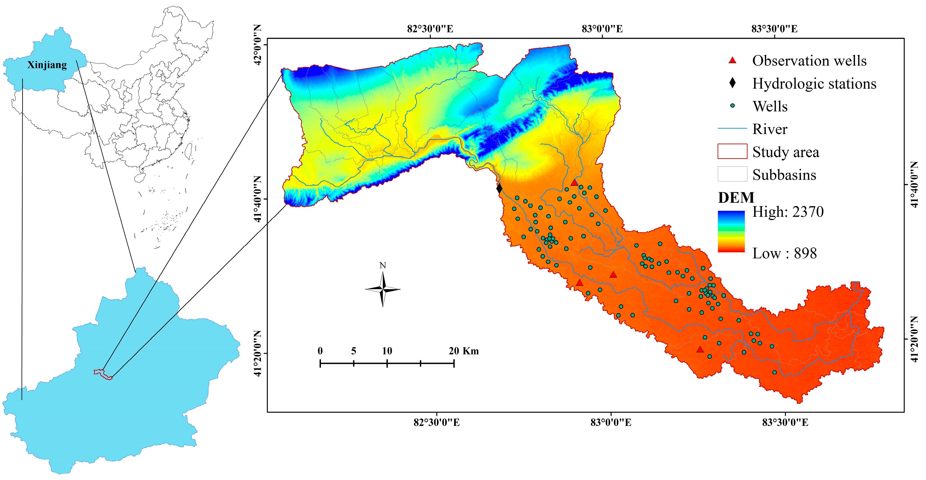
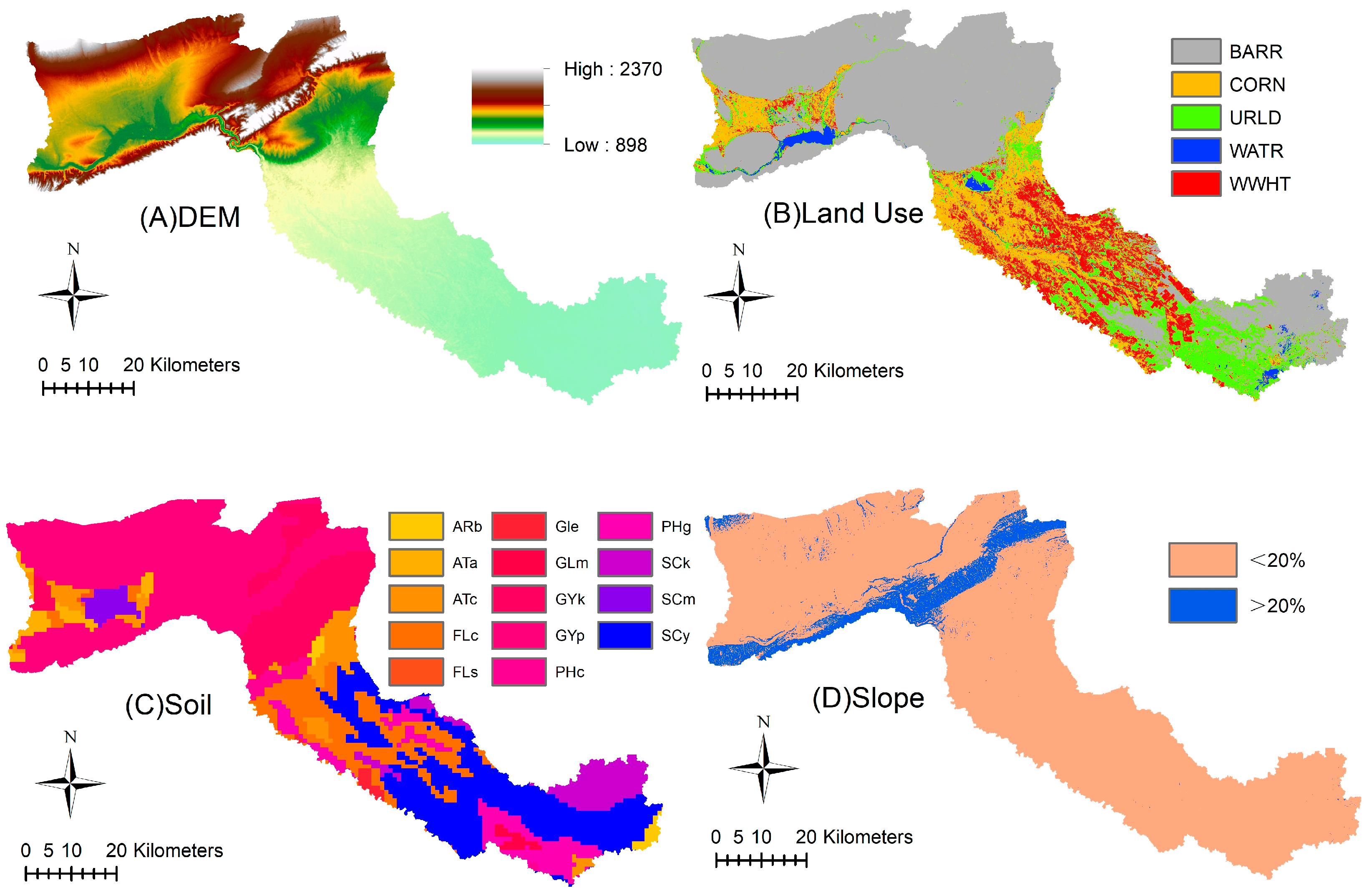
2.1. Research Area
2.2. SWAT Model
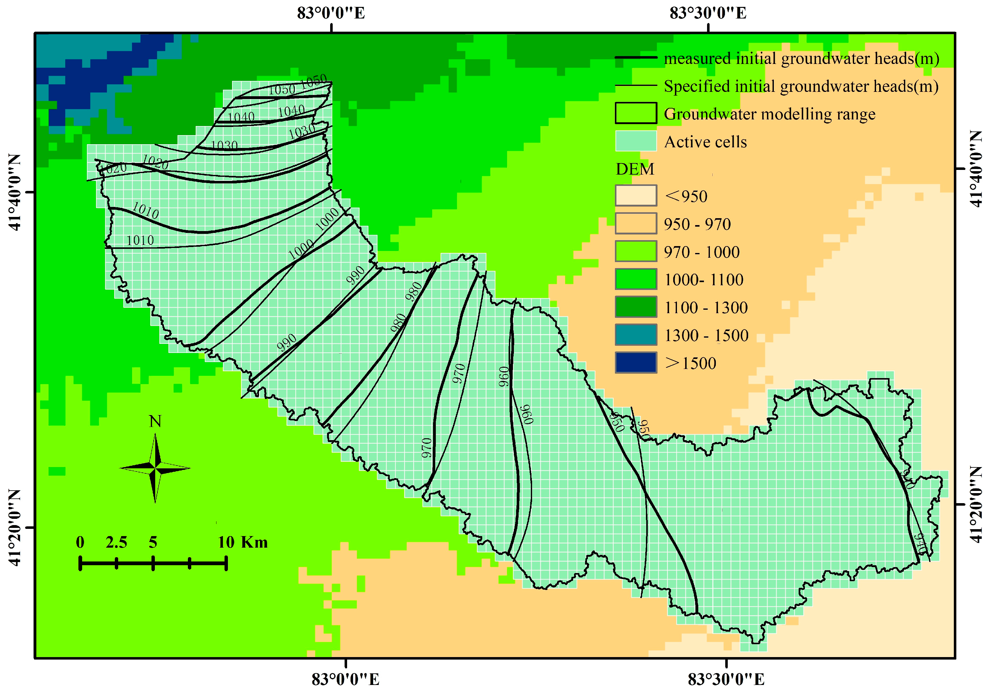
2.3. MODFLOW Model
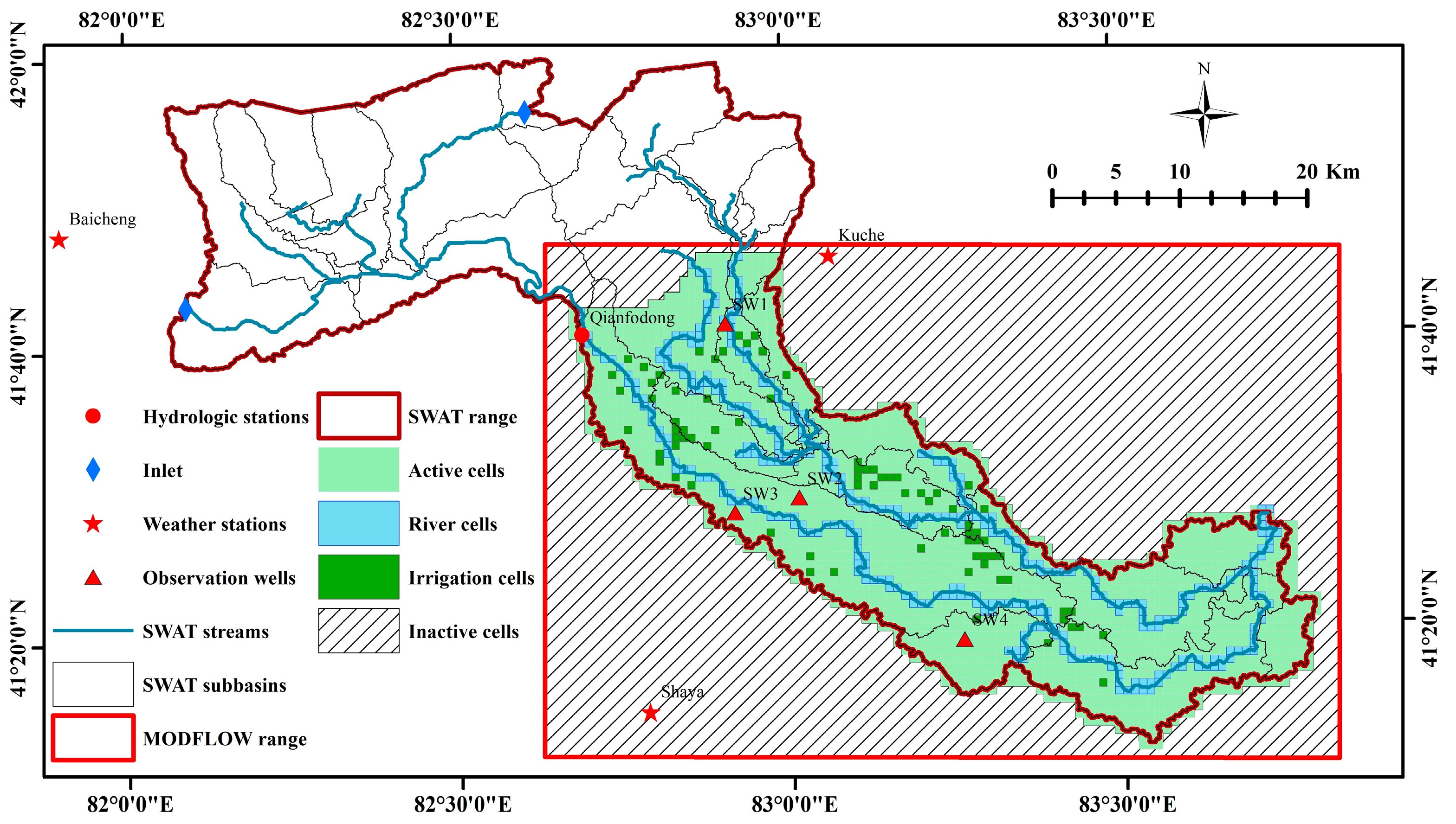
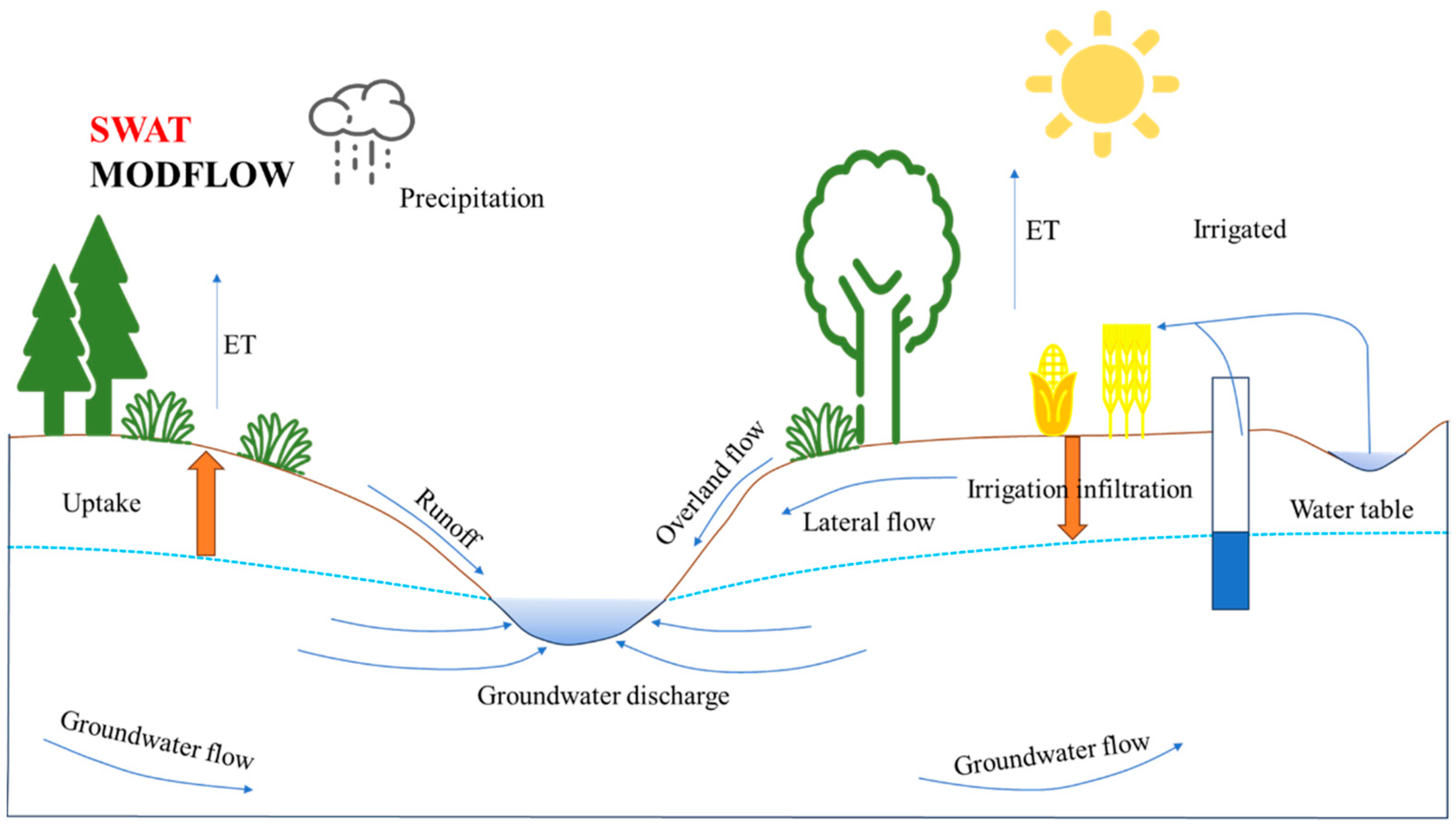
2.4. Coupling of SWAT and MODFLOW
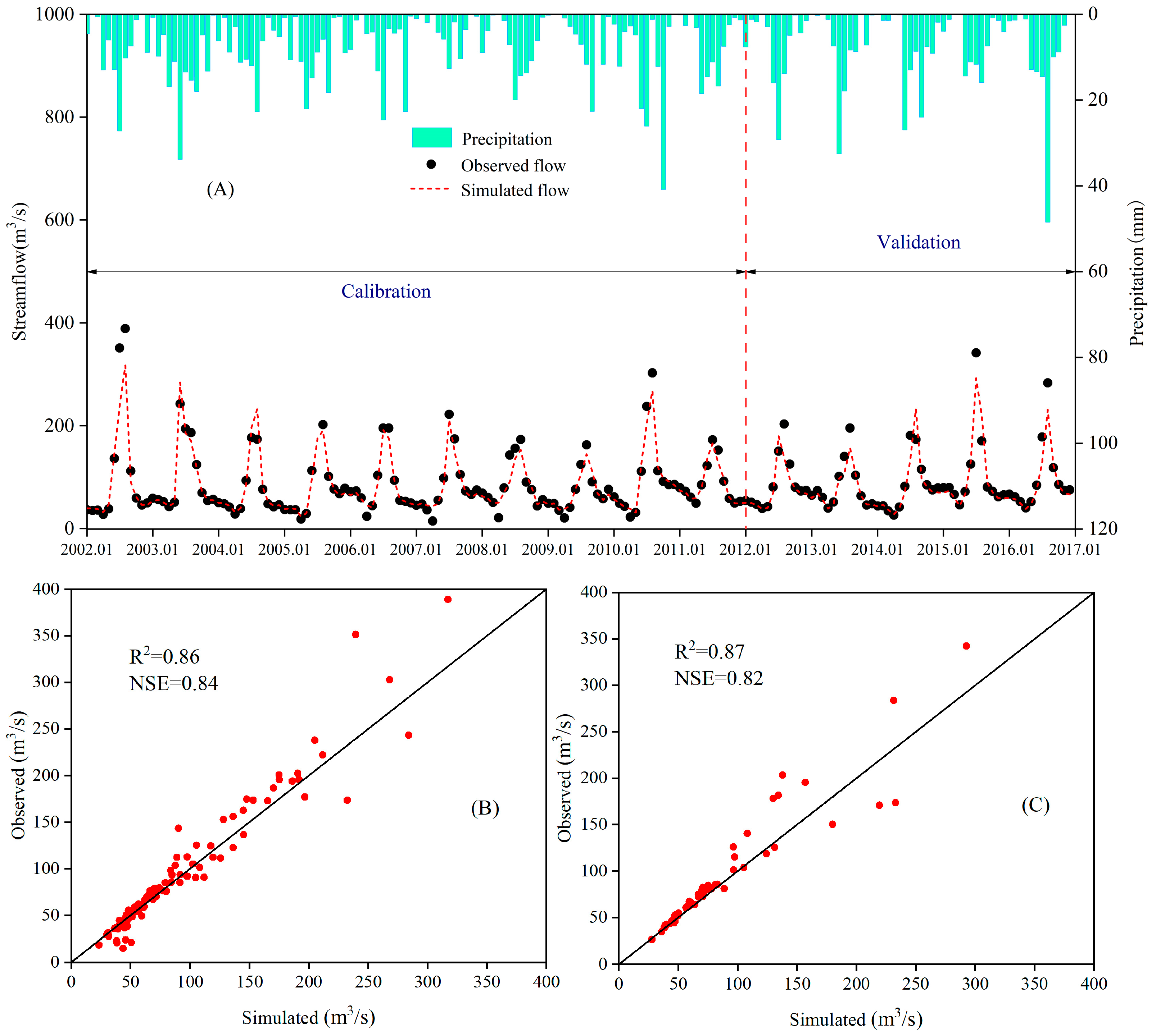
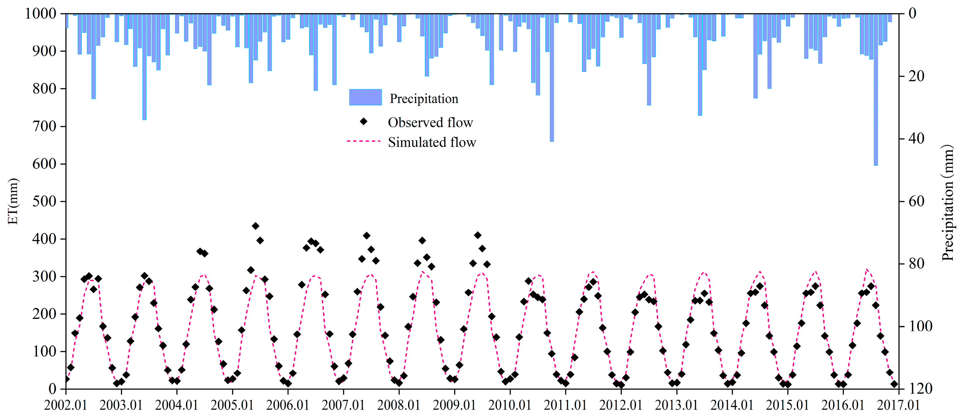
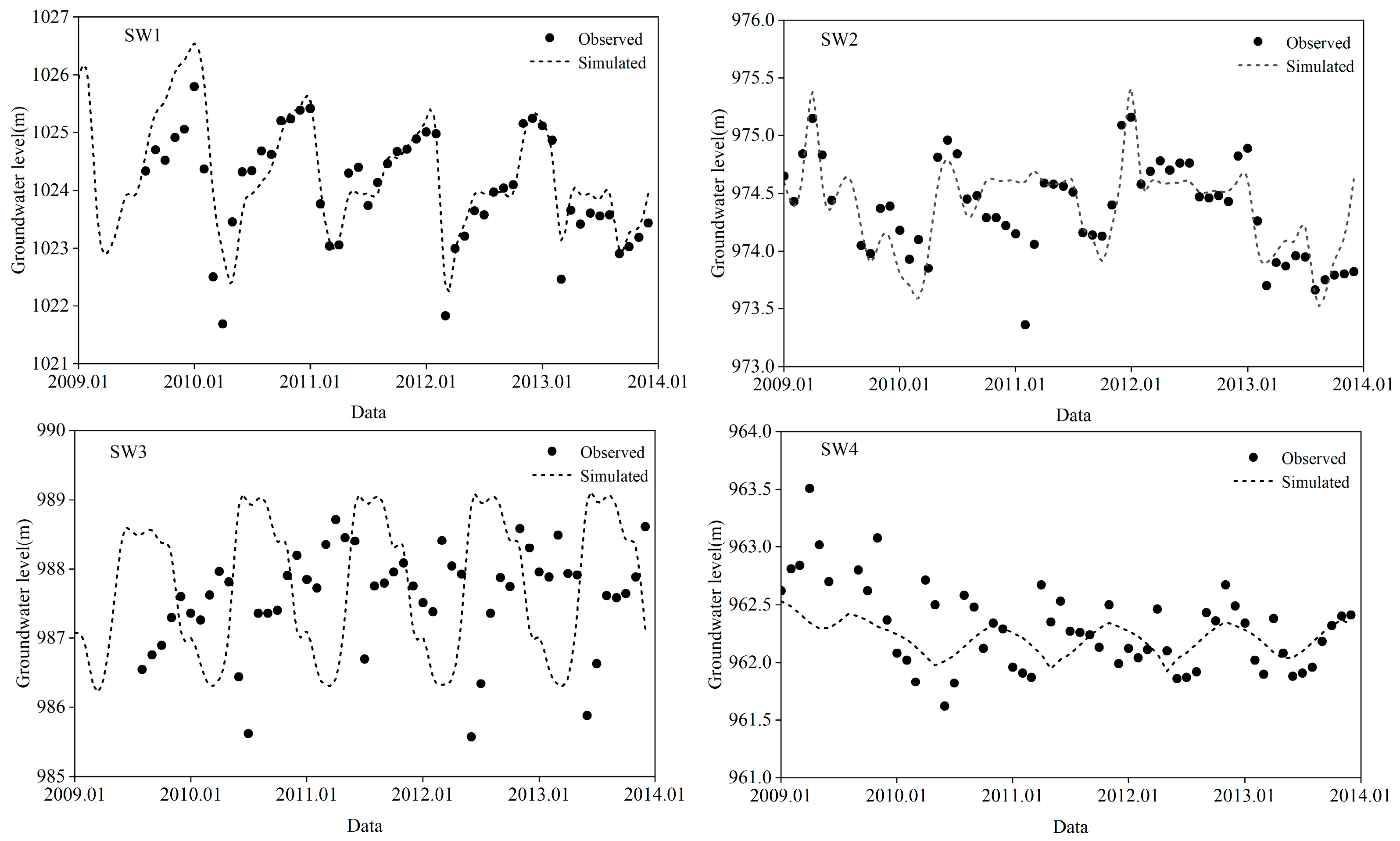
2.5. Calibration and Validation of the Model
3. Results and Discussion
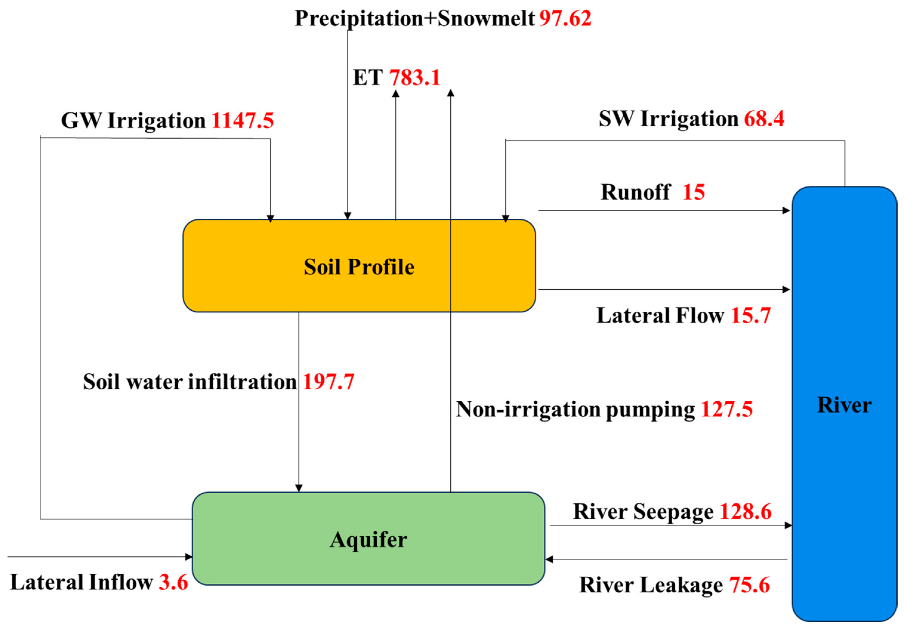
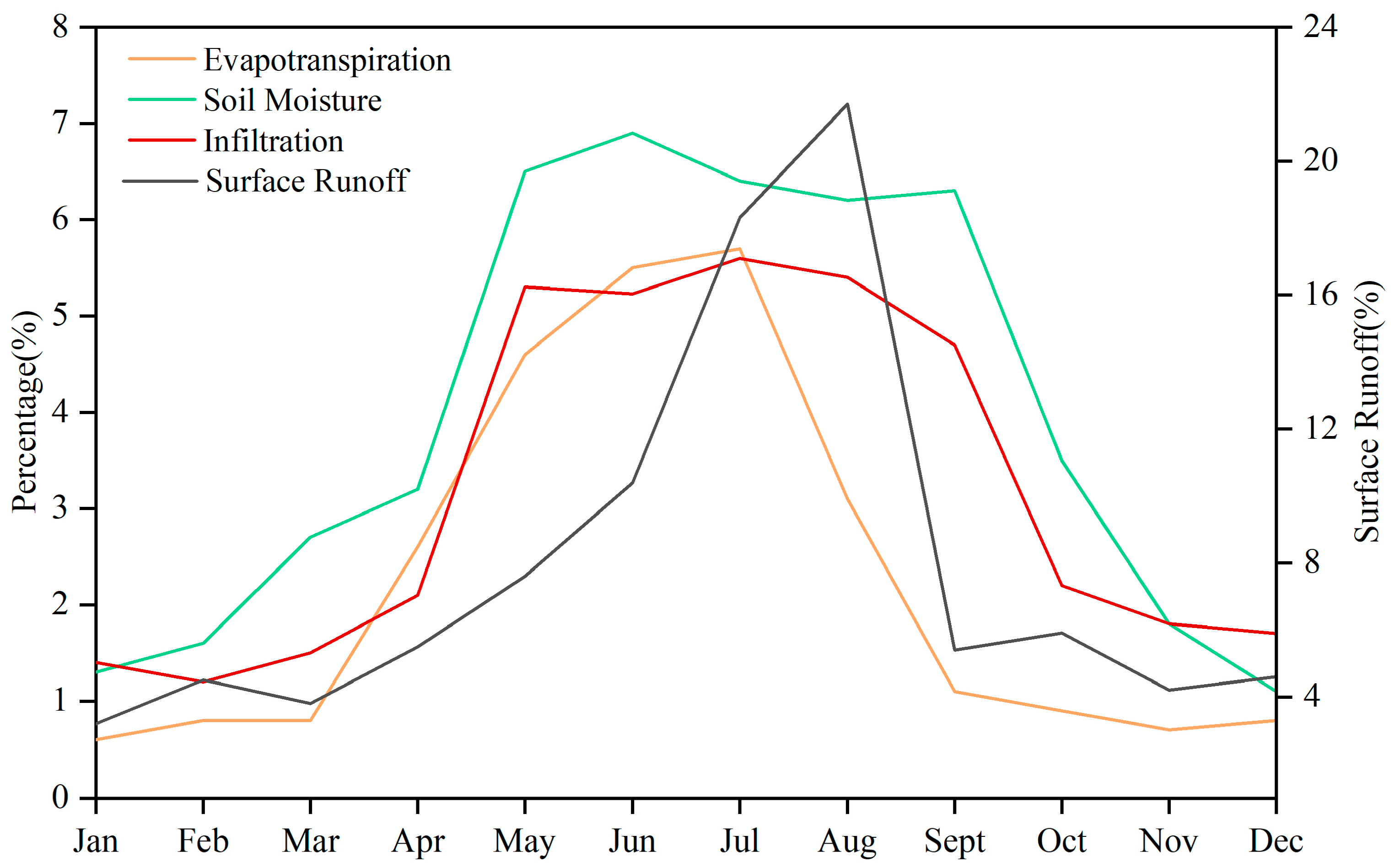
3.1. Water Balance and Hydrological Response Analysis under Irrigation Activities
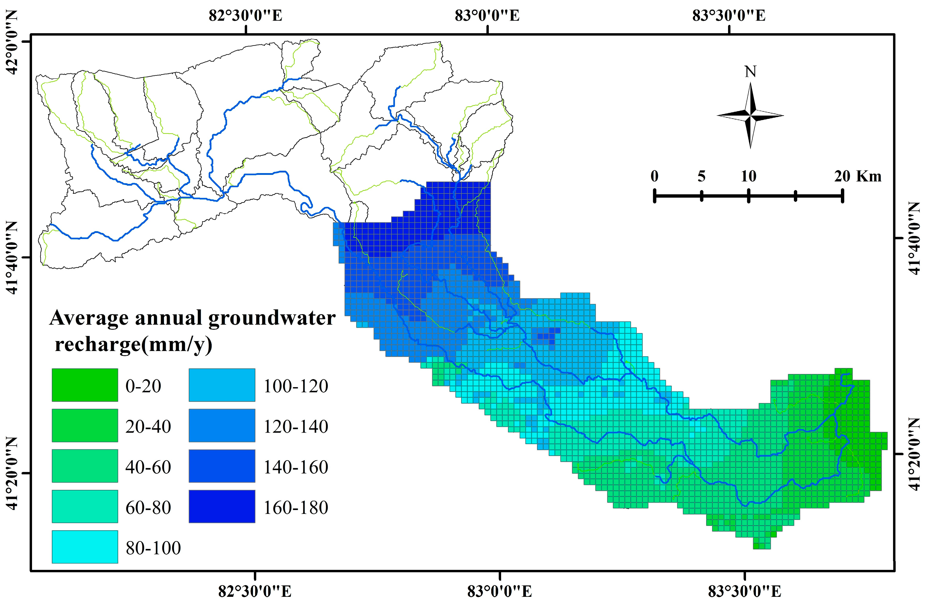
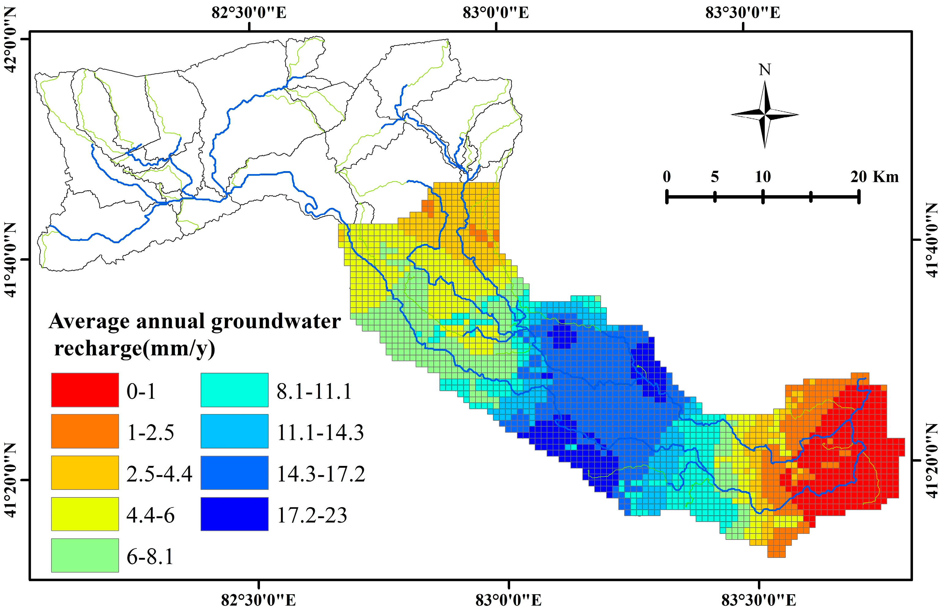
3.2. Impact of Irrigation Activities on Groundwater Recharge
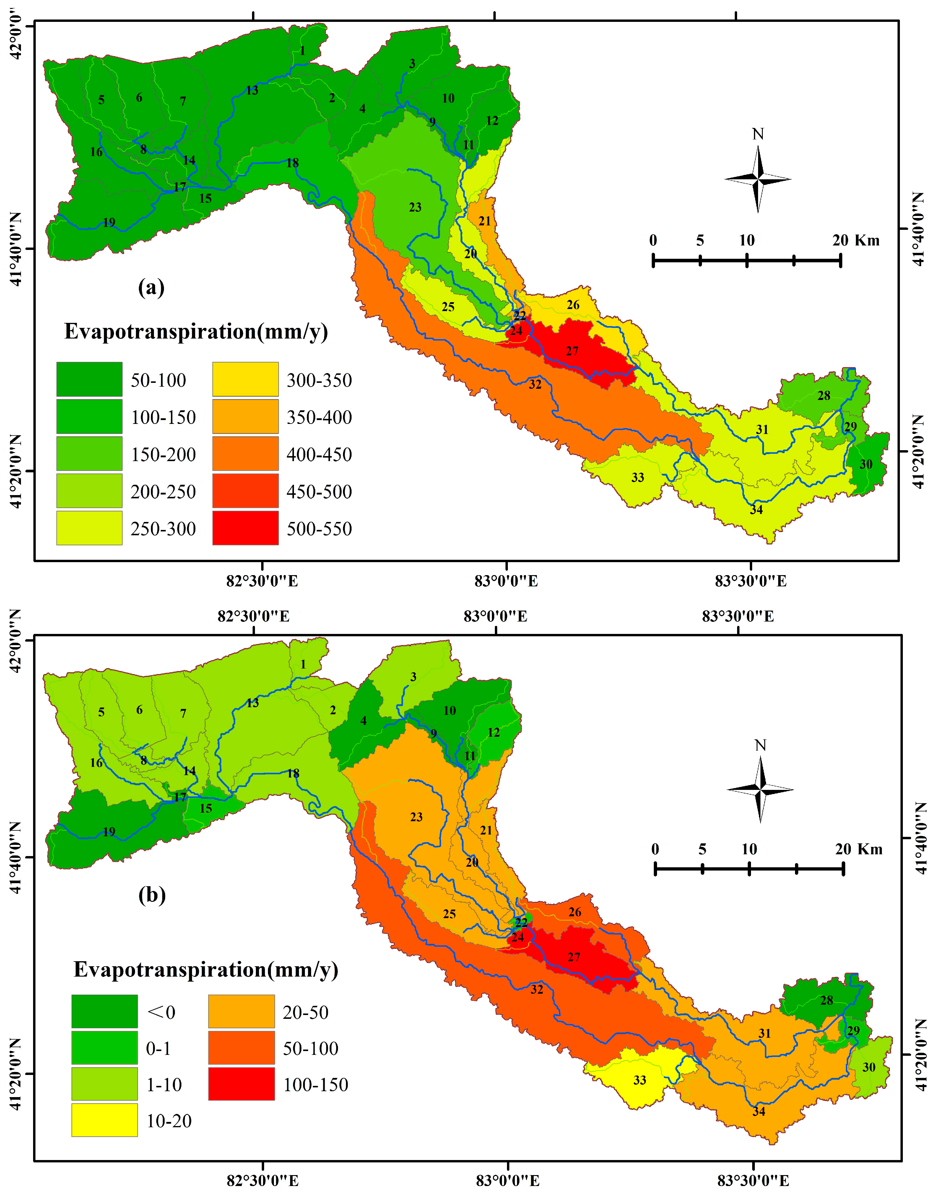
3.3. Impact of Irrigation Activities on Evaporation
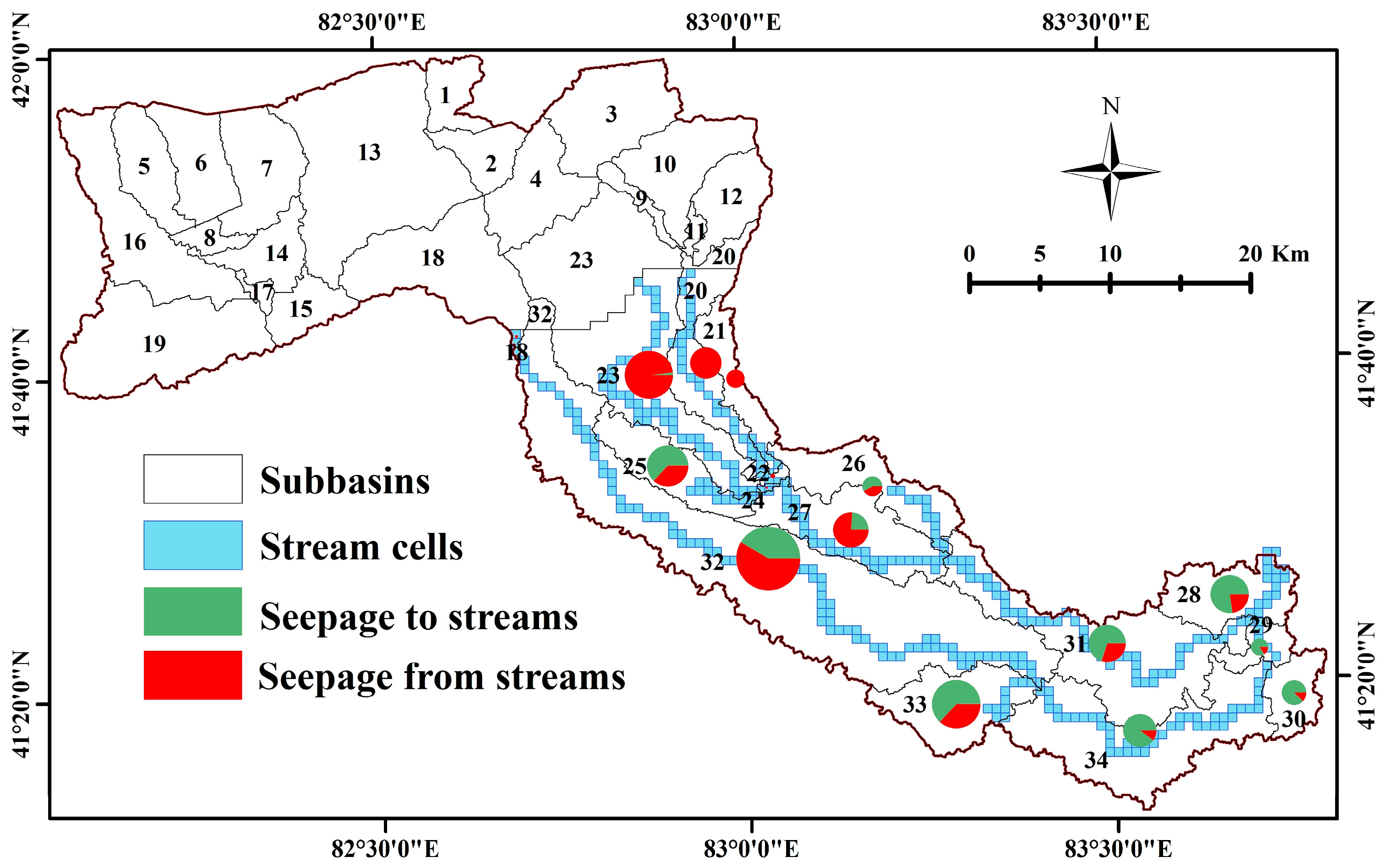
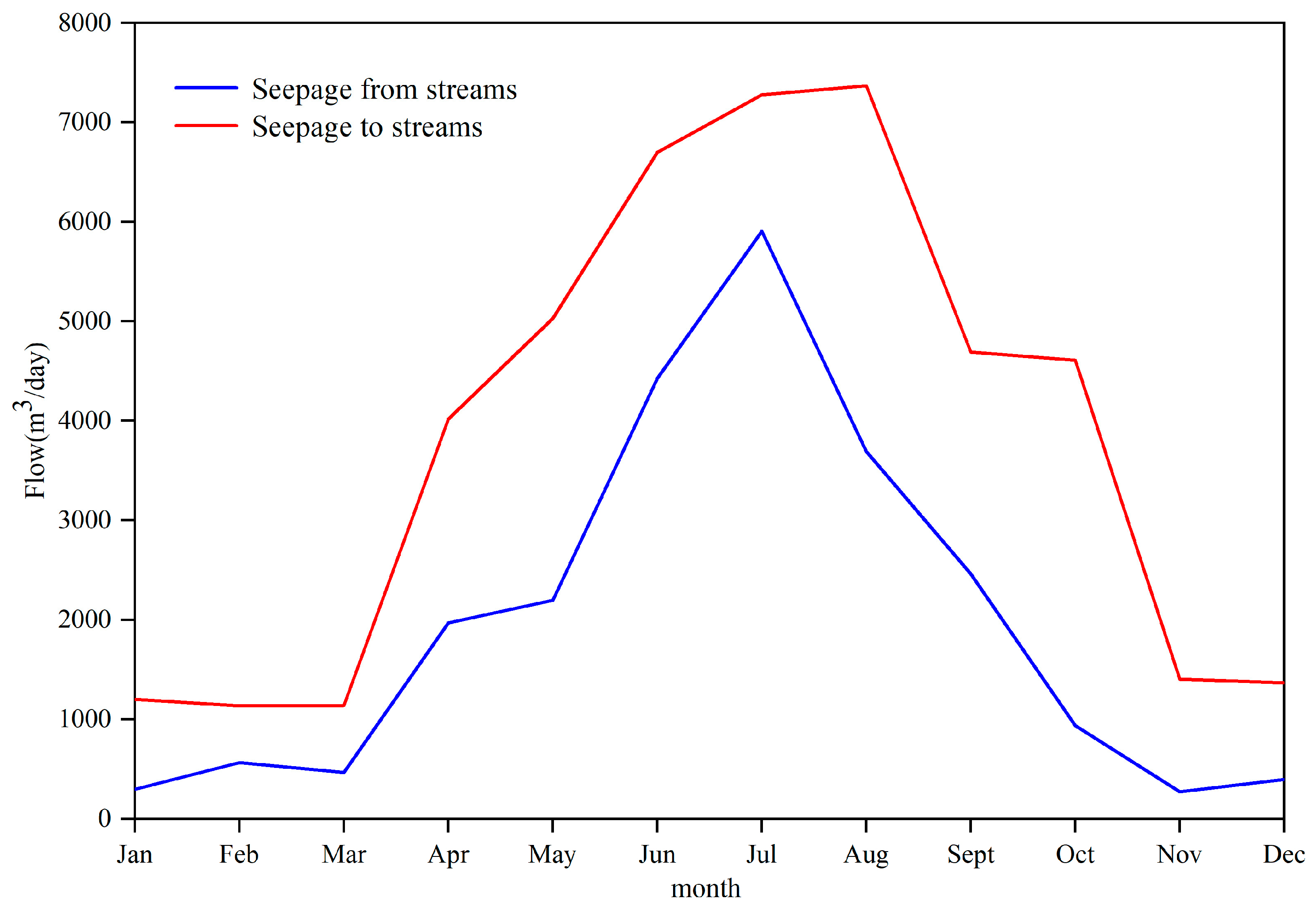
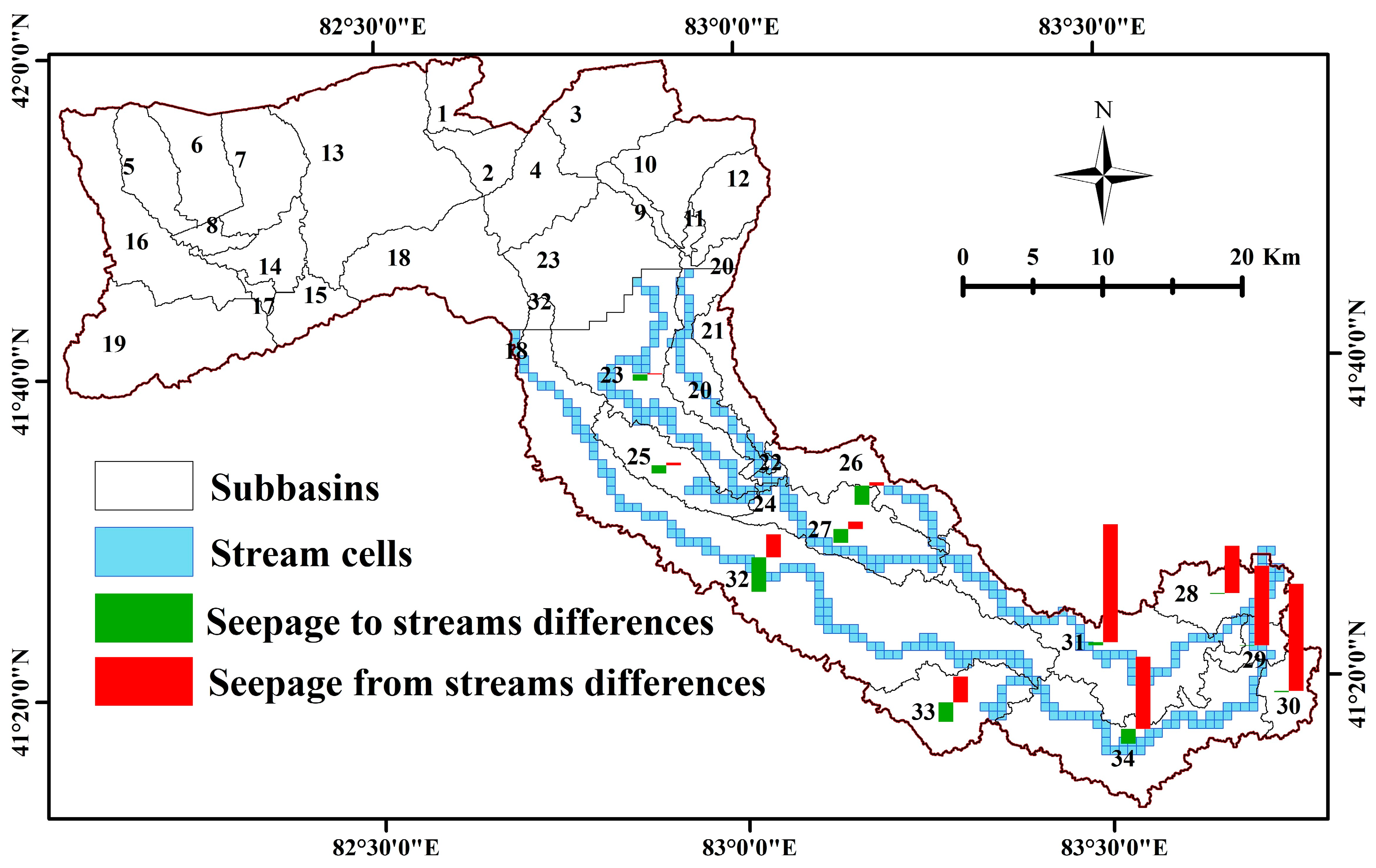
3.4. Impact of Irrigation Activities on the Exchange of Surface Water and Groundwater
4. Conclusions
Author Contributions
Funding
Data Availability Statement
Acknowledgments
Conflicts of Interest
References
- Khokhar, T. Chart: Globally, 70% of Freshwater is Used for Agriculture. World Bank Data Blog. 2017. Available online: https://blogs.worldbank.org/opendata/chart-globally-70-freshwater-used-agriculture. (accessed on 6 August 2023).
- Frenken, K.; Gillet, V. Irrigation Water Requirement and Water Withdrawal by Country; Food and Agriculture Organization (FAO) of the United Nations: Rome, Italy, 2012. [Google Scholar]
- Samimi, M.; Mirchi, A.; Moriasi, D.; Ahn, S.; Alian, S.; Taghvaeian, S.; Sheng, Z. Modeling Arid/Semi-arid Irrigated Agricultural Watersheds with SWAT: Applications, Challenges, and Solution Strategies. J. Hydrol. 2020, 590, 125418. [Google Scholar] [CrossRef]
- AghaKouchak, A.; Feldman, D.; Hoerling, M.; Huxman, T.; Lund, J. Water and climate: Recognize anthropogenic drought. Nature 2015, 524, 409–411. [Google Scholar] [CrossRef] [PubMed]
- Sun, C.-Z.; Wei, Y.-Q.; Zhao, L.-S. Co-evolution of water-energy-food nexus in arid areas: Take Northwest China as an example. J. Nat. Resour. 2022, 37, 320–333. [Google Scholar] [CrossRef]
- Zhu, L.; Xia, X.-X.; Yang, A.-M.; Jin, H. Expansion of cultivated land in the oasis area of the Manas River Basin sensitivity analysis of CA-Markov model parameters. Arid Zone Res. 2020, 37, 1327–1336. [Google Scholar]
- Yan, X.; Wang, Y.; Chen, Y.; Yang, G.; Xia, B.; Xu, H. Study on the Spatial Allocation of Receding Land and Water Reduction under Water Resource Constraints in Arid Zones. Agriculture 2022, 12, 926. [Google Scholar] [CrossRef]
- Lankford, B.; Pringle, C.; McCosh, J.; Shabalala, M.; Hess, T.; Knox, J.W. Irrigation area, efficiency and water storage mediate the drought resilience of irrigated agriculture in a semi-arid catchment. Sci. Total Environ. 2022, 859, 160623. [Google Scholar] [CrossRef]
- Han, C.; Zhang, B.; Han, S. Quantitative effects of changes in agricultural irrigation on potential evaporation. Hydrol. Process. 2021, 35, e14057. [Google Scholar] [CrossRef]
- Nakayama, T. Simulation of the effect of irrigation on the hydrologic cycle in the highly cultivated Yellow River Basin. Agric. For. Meteorol. 2010, 151, 314–327. [Google Scholar] [CrossRef]
- Wei, X.; Garcia-Chevesich, P.; Alejo, F.; García, V.; Martínez, G.; Daneshvar, F.; Bowling, L.C.; Gonzáles, E.; Krahenbuhl, R.; McCray, J.E. Hydrologic Analysis of an Intensively Irrigated Area in Southern Peru Using a Crop-Field Scale Framework. Water 2021, 13, 318. [Google Scholar] [CrossRef]
- Shu, Y.; Villholth, K.G.; Jensen, K.H.; Stisen, S.; Lei, Y. Integrated hydrological modeling of the North China Plain: Options for sustainable groundwater use in the alluvial plain of Mt. Taihang. J. Hydrol. 2012, 464–465, 79–93. [Google Scholar] [CrossRef]
- Liu, J.; Zhou, Z.; Yan, Z.; Gong, J.; Jia, L.; Xu, C.Y.; Wang, H. A new approach to separating the impacts of climate change and multiple human activities on water cycle processes based on a distributed hydrological model. J. Hydrol. 2019, 578, 124096. [Google Scholar] [CrossRef]
- Li, H.; Zhang, Q.; Singh, V.P.; Shi, P.; Sun, P. Hydrological effects of cropland and climatic changes in arid and semi-arid river basins: A case study from the Yellow River basin, China. J. Hydrol. 2017, 549, 547–557. [Google Scholar] [CrossRef]
- Arnold, J.G.; Srinivasan, R.; Muttiah, R.S.; Williams, J.R. Large area hydrologic modeling and assessment part I: Model development. J. Am. Water Resour. Assoc. 1998, 34, 73–89. [Google Scholar] [CrossRef]
- McDonald, M.; Harbaugh, A.W. A Modular Three-Dimensional Finite-Difference GroundWater Flow Model; U.S. Geological Survey: Reston, WV, USA, 1988.
- Guevara Ochoa, C.; Medina Sierra, A.; Vives, L.; Zimmermann, E.; Bailey, R. Spatio-temporal patterns of the interaction between groundwater and surface water in plains. Hydrol. Process. 2020, 34, 1371–1392. [Google Scholar] [CrossRef]
- George, A.; Hoang, T.L.; Takashi, G. A Review of SWAT Model Application in Africa. Water 2021, 13, 1313. [Google Scholar]
- Wagner, P.D.; Bieger, K.; Arnold, J.G.; Fohrer, N. Representation of hydrological processes in a rural lowland catchment in Northern Germany using SWAT and SWAT+. Hydrol. Process. 2022, 36, e14589. [Google Scholar] [CrossRef]
- Castellanos-Osorio, G.; López-Ballesteros, A.; Pérez-Sánchez, J.; Senent-Aparicio, J. Disaggregated monthly SWAT+ model versus daily SWAT+ model for estimating environmental flows in Peninsular Spain. J. Hydrol. 2023, 623, 129837. [Google Scholar] [CrossRef]
- Wen, J.; Wang, S.; Wang, H.; Cui, Y. Study on water cycle simulation model of multi-sources and multi-functional irrigation area based on SWAT model (II): Application of Wanyao irrigation area. IOP Conf. Ser. Earth Environ. Sci. 2020, 510, 032019. [Google Scholar] [CrossRef]
- Xu, X.Z. Assessment of runoff and sediment yield in the Miyun Reservoir catchment by using SWAT model. Hydrol. Process. 2009, 23, 3619–3630. [Google Scholar] [CrossRef]
- Rasmus, F.R.; Eugenio, M. The importance of subsurface drainage on model performance and water balance in an agricultural catchment using SWAT and SWAT-MODFLOW. Agric. Water Manag. 2021, 255, 107058. [Google Scholar]
- Fu, X. Optimization Management of Groundwater Resources and Modeling and Reme-diation of Nitrate Pollution in YangZhuang Basin; China University of Geosciences: Wuhan, China, 2019. [Google Scholar]
- Zheng, Z. Coupling Simulation of Surface Water and Groundwater in Beishan Reservoir Watershed Based on SWAT-MODFLOW; Nanjing University: Nanjing, China, 2021. [Google Scholar]
- Bailey, R.T.; Wible, T.C.; Arabi, M.; Records, R.M.; Ditty, J. Assessing regional-scale spatio-temporal patterns of groundwater–surface water interactions using a coupled SWAT-MODFLOW model. Hydrol. Process. 2016, 30, 4420–4433. [Google Scholar] [CrossRef]
- Molina-Navarro, E.; Bailey, R.T.; Andersen, H.E.; Thodsen, H.; Nielsen, A.; Park, S.; Jensen, J.S.; Jensen, J.B.; Trolle, D. Comparison of abstraction scenarios simulated by SWAT and SWAT-MODFLOW. Hydrol. Sci. J. 2019, 64, 434–454. [Google Scholar] [CrossRef]
- Liu, W.; Park, S.; Bailey, R.T.; Molina-Navarro, E.; Andersen, H.E.; Thodsen, H.; Nielsen, A.; Jeppesen, E.; Jensen, J.S.; Trolle, D. Quantifying the streamflow response to groundwater abstractions for irrigation or drinking water at catchment scale using SWAT and SWAT–MODFLOW. Environ. Sci. Eur. 2020, 32, 1–25. [Google Scholar] [CrossRef]
- Chunn, D.; Faramarzi, M.; Smerdon, B.; Alessi, D.S. Application of an Integrated SWAT–MODFLOW Model to Evaluate Potential Impacts of Climate Change and Water Withdrawals on Groundwater–Surface Water Interactions in West-Central Alberta. Water 2019, 11, 110. [Google Scholar] [CrossRef]
- Aliyari, F.; Bailey, R.T.; Tasdighi, A.; Dozier, A.; Arabi, M.; Zeiler, K. Coupled SWAT-MODFLOW model for large-scale mixed agro-urban river basins. Environ. Model. Softw. 2019, 115, 200–210. [Google Scholar] [CrossRef]
- Jafari, T.; Kiem, A.S.; Javadi, S.; Nakamura, T.; Nishida, K. Fully integrated numerical simulation of surface water-groundwater interactions using SWAT-MODFLOW with an improved calibration tool. J. Hydrol. Reg. Stud. 2021, 35, 100822. [Google Scholar] [CrossRef]
- Li, L. Spatial distribution and variation characteristics of soil salinity in the oasis of Weigan and Kuqa rivers. J. Arid Land Resour. Environ. 2022, 36, 136–142. [Google Scholar]
- Jiang, M. Interaction between Groundwater and Surface Water under Large-Scale Exploitation Conditions Based on SWAT-MODFLOW Model; Lanzhou University: Lanzhou, China, 2021. [Google Scholar]
- Yifru, B.A.; Chung, I.-M.; Kim, M.-G.; Chang, S.W. Assessment of Groundwater Recharge in Agro-Urban Watersheds Using Integrated SWAT-MODFLOW Model. Sustainability 2020, 12, 6593. [Google Scholar] [CrossRef]
- Park, S.; Nielsen, A.; Bailey, R.T.; Trolle, D.; Bieger, K. A QGIS-based graphical user interface for application and evaluation of SWAT-MODFLOW models. Environ. Model. Softw. 2018, 111, 493–497. [Google Scholar] [CrossRef]
- Wei, X.; Bailey, T.R. Assessment of System Responses in Intensively Irrigated Stream–Aquifer Systems Using SWAT-MODFLOW. Water 2019, 11, 1576. [Google Scholar] [CrossRef]
- Dangol, S.; Zhang, X.; Liang, X.Z.; Miralles-Wilhelm, F. Agricultural Irrigation Effects on Hydrological Processes in the United States Northern High Plains Aquifer Simulated by the Coupled SWAT-MODFLOW System. Water 2022, 14, 1938. [Google Scholar] [CrossRef]
- Chen, Z. Simulation of Interaction between Surface Water and Groundwater and Evaluation of Nitrate Load in Shaying River Sasin; Nanjing University: Nanjing, China, 2017. [Google Scholar]

| Data Type | Scale or Spatial Resolution | Data Sources |
|---|---|---|
| Elevation | 90 m | Spatial geographic data cloud |
| Land-use map | 30 m | GlobeLand30, LANDSAT8 |
| Soil | 10 km | FAO Digital Soil Map of the World |
| Weather | 0.25° × 0.25° | China Meteorological Data Network |
| Streamflow | monthly scale | Xinjiang Water Conservancy and Hydropower Survey and Design Institute |
| Irrigation system | field investigation |
| Crop type | Management Operations | Operating Time | Irrigation Water Volume (mm) | Irrigation Method |
|---|---|---|---|---|
| winter wheat | plantation | 25 September | ||
| harvest | 28 May | |||
| irrigated | 15 March | 120 | diffusion irrigation | |
| 20 April | 120 | diffusion irrigation | ||
| 20 May | 120 | diffusion irrigation | ||
| 18 September | 120 | diffusion irrigation | ||
| 20 November | 135 | diffusion irrigation | ||
| cotton | plantation | 1 June | ||
| harvest | 15 September | |||
| irrigated | 10 June | 22.5 | drip irrigation | |
| 25 June | 37.5 | drip irrigation | ||
| 10 July | 30 | drip irrigation | ||
| 22 July | 30 | drip irrigation | ||
| 25 August | 30 | drip irrigation | ||
| corn | plantation | 20 March | ||
| harvest | 25 September | |||
| irrigated | 22 March | 120 | diffusion irrigation | |
| 25 May | 105 | diffusion irrigation | ||
| 20 June | 97.4 | diffusion irrigation | ||
| 27 July | 97.4 | diffusion irrigation | ||
| 11 August | 90 | diffusion irrigation |
| Parameter Name | Definition | t-Stat | p-Value | Value Range |
|---|---|---|---|---|
| V__TRNSRCH.bsn | Fraction of transmission losses from main channel that enters deep aquifer | −42.61 | 0 | 0–1 |
| V__CH_K2.rte | Effective hydraulic conductivity in main channel alluvium | −11.9 | 0 | 0.01–150 |
| IRR_EFF.mgt | Irrigation efficiency | −8.66 | 0 | 0–1 |
| V__CNCOEF.bsn | Plant ET curve number coefficient | −1.86 | 0.06 | 0–2 |
| V__ALPHA_BNK.rte | Baseflow alpha factor for bank storage | 1.78 | 0.08 | 0–1.5 |
| V__CH_N2.rte | Manning’s n value for the main channel | −1.69 | 0.09 | 0–1 |
| V__SOL_AWC.sol | Available water capacity of the soil layer | −1.61 | 0.11 | 0.03–0.5 |
| V__SOL_K.sol | Saturated hydraulic conductivity | −1.50 | 0.13 | 1–100 |
| V__DEP_IMP.hru | Depth to impervious layer for modeling of perched water tables | −1.36 | 0.17 | 0–1000 |
| V__SURLAG.bsn | Surface runoff lag time | 1.26 | 0.21 | 1–10 |
| V__EPCO.hru | Plant uptake compensation factor | 1.22 | 0.22 | 0–1.5 |
| V__CH_S1.sub | Average slope of tributary channels | −1.11 | 0.27 | −0.2–0.2 |
| V__ALPHA_BF.gw | Baseflow alpha factor | 1.05 | 0.29 | 0–1 |
| V__RCHRG_DP.gw | Deep aquifer percolation fraction | −1.03 | 0.30 | 0–30 |
| V__CN2.mgt | Soil conservation service (SCS) runoff curve number | −0.97 | 0.33 | −0.2–0.2 |
Disclaimer/Publisher’s Note: The statements, opinions and data contained in all publications are solely those of the individual author(s) and contributor(s) and not of MDPI and/or the editor(s). MDPI and/or the editor(s) disclaim responsibility for any injury to people or property resulting from any ideas, methods, instructions or products referred to in the content. |
© 2023 by the authors. Licensee MDPI, Basel, Switzerland. This article is an open access article distributed under the terms and conditions of the Creative Commons Attribution (CC BY) license (https://creativecommons.org/licenses/by/4.0/).
Share and Cite
Liang, F.; Li, S.; Jie, F.; Ge, Y.; Liu, N.; Jia, G. The Development of a Coupled Soil Water Assessment Tool-MODFLOW Model for Studying the Impact of Irrigation on a Regional Water Cycle. Water 2023, 15, 3542. https://doi.org/10.3390/w15203542
Liang F, Li S, Jie F, Ge Y, Liu N, Jia G. The Development of a Coupled Soil Water Assessment Tool-MODFLOW Model for Studying the Impact of Irrigation on a Regional Water Cycle. Water. 2023; 15(20):3542. https://doi.org/10.3390/w15203542
Chicago/Turabian StyleLiang, Fuli, Sheng Li, Feilong Jie, Yanyan Ge, Na Liu, and Guangwei Jia. 2023. "The Development of a Coupled Soil Water Assessment Tool-MODFLOW Model for Studying the Impact of Irrigation on a Regional Water Cycle" Water 15, no. 20: 3542. https://doi.org/10.3390/w15203542
APA StyleLiang, F., Li, S., Jie, F., Ge, Y., Liu, N., & Jia, G. (2023). The Development of a Coupled Soil Water Assessment Tool-MODFLOW Model for Studying the Impact of Irrigation on a Regional Water Cycle. Water, 15(20), 3542. https://doi.org/10.3390/w15203542