Article

Retrieving Eutrophic Water in Highly Urbanized Area Coupling UAV Multispectral Data and Machine Learning Algorithms

1
State Key Laboratory of Subtropical Building Science, School of Civil Engineering and Transportation, South China University of Technology, Guangzhou 510641, China
2
Pazhou Lab, Guangzhou 510335, China
*
Author to whom correspondence should be addressed.
Water 2023, 15(2), 354; https://doi.org/10.3390/w15020354
Submission received: 15 November 2022 / Revised: 16 December 2022 / Accepted: 30 December 2022 / Published: 14 January 2023
(This article belongs to the Special Issue Application of AI and UAV Techniques in Urban Water Science)

Abstract

:
With the rapid development of urbanization and a population surge, the drawback of water pollution, especially eutrophication, poses a severe threat to ecosystem as well as human well-being. Timely monitoring the variations of water quality is a precedent to preventing the occurrence of eutrophication. Traditional monitoring methods (station monitoring or satellite remote sensing), however, fail to real-time obtain water quality in an accurate and economical way. In this study, an unmanned aerial vehicle (UAV) with a multispectral camera is used to acquire the refined remote sensing data of water bodies. Meanwhile, in situ measurement and sampling in-lab testing are carried out to obtain the observed values of four water quality parameters; subsequently, the comprehensive trophic level index (TLI) is calculated. Then three machine learning algorithms (i.e., Extreme Gradient Boosting (XGB), Random Forest (RF) and Artificial Neural Network (ANN)) are applied to construct the inversion model for water quality estimation. The measured values of water quality showed that the trophic status of the study area was mesotrophic or light eutrophic, which was consistent with the government’s water-control ambition. Among the four water quality parameters, TN had the highest correlation (r = 0.81, p = 0.001) with TLI, indicating that the variation in TLI was inextricably linked to TN. The performances of the three models were satisfactory, among which XGB was considered the optimal model with the best accuracy validation metrics (R2 = 0.83, RMSE = 0.52). The spatial distribution map of water quality drawn by the XGB model was in good agreement with the actual situation, manifesting the spatial applicability of the XGB model inversion. The research helps guide effective monitoring and the development of timely warning for eutrophication.

1. Introduction

In the past century, due to the urban and industrial expansion, severe eutrophication has become an important problem faced by urban water bodies worldwide [1,2,3,4]. In China, a developing country, the problem is particularly acute in places with rapid process of industrialization [5], such as the Great Bay Area [6,7]. In 2019, data from the nutritional status monitoring of 107 major lakes/reservoirs in China showed that 62.36% were in middle eutropher status and 22.40% were in light eutropher status [8]. To solve a series of water environmental problems, the Action Plan for Prevention and Control of Water Pollution was carried out by the government in 2015, which has achieved some results. However, algal blooms caused by eutrophication still occur from time to time, destroying the ecological balance of the region and affecting the quality of drinking water, influencing the production and life of human beings [1,9,10,11]. Therefore, it is necessary to monitor water quality so that timely measures can be taken to prevent eutrophication.
The traditional water quality monitoring method is to collect water samples manually and then use chemical experiments to obtain accurate nutritional indicators. This approach has high accuracy but complicated operation and low efficiency [12]. In addition, errors caused by the difference of laboratory instruments, analysis methods and human resources and the non-real-time data acquisition are the problems it faced [13]. In order to solve the above problems, ADu-Manu et al. proposed a new method for water quality monitoring systems by using a wireless sensor network [14]. Depending on the size of the water bodies and the purpose of monitoring, different network topologies and node densities are adopted at first, and different types of sensors are placed at the water source to access physical and chemical parameters. This method can meet the requirements of high data precision, data accuracy and timely reporting well [15], but it is high cost, not flexible enough and only used for a single target [16].
By contrast, remote sensing is a cheaper and more universal method, which depends on the connection between the spectral reflectance of water bodies and water quality parameters [15]. Most previous studies used satellite-based platforms for monitoring, such as Landsat Thematic Mapper [17,18], Sentinel-2 [19,20], Operational Land Imager [21,22] and the Moderate Resolution Imaging Spectrometer [5,23]. The specific method is to obtain the multispectral reflectance data by processing the satellite images, and meanwhile take samples on site to analyze water quality and then find a relationship between the measured water quality parameters and multispectral data. However, because of the shortcomings of coarse spatial resolution, satellite remote sensing is not optimal for most small and scattered urban waters. At the same time, larger interference from the atmosphere and the more complex optical characteristics of inland waters compared with oceanic waters narrow the application of satellites [24,25]. Besides, due to a long revisit period, satellite remote sensing cannot monitor timely to master real-time water quality information after sudden changes of meteorological factors or algal blooms in a short period.
Therefore, a method for urban water quality monitoring using unmanned aerial vehicle (UAV) platforms were proposed, using a UAV carrying multi-spectral sensors to obtain the spectral information of water bodies as the input data to build water-quality models [26,27]. UAVs have the advantages of the above two approaches, which means they are not only more cost-effective, but also more flexible and portable, grasping the change in water quality with a short revisit period [28]. At the same time, the data obtained by UAVs is more accurate because of the low-altitude flight, which is suitable for small and fragmented urban water bodies. Due to these advantages, UAVs have been widely used to retrieve various water quality parameters in previous studies.
After obtaining remote sensing data, bio-optical models are used to analyze the water components. The models can be roughly divided into analytical methods and empirical methods [29,30,31]. The former is to use the theory of radiation transfer to deduce the optical characteristics of each component in the water column, which extends the semi-analytical methods and quasi-analytical methods, generally used to estimate concentrations of chlorophyll-a(Chl-a), total suspended solids and other optically active substances [29]. For example, Lee et al. put forward a quasi-analytical model for Chl-a in class II water in 2002 [32]. Subsequently, in 2013, Li et al. reparameterized and proposed the IIMIV model, which was used to retrieve Chl-a concentrations [33]. Instead of using onboard multispectral cameras as sensors, these methods typically use optical sensors with more specific spectral information, such as spectrophotometers or ocean optics in situ sensors [33,34]. In contrast, empirical methods are to establish the relationship between water quality parameters and radiation data through statistical analysis rather than physical or optical principles [29,35,36], which are suitable methods for this study considering the complexity of the inland water composition.
With the progression of algorithms, the statistical analysis models used in empirical methods are also improving, with higher accuracy and universality [35]. In 2001, Cheng and Lei used multiple linear regression models to construct relationships between Landsat TM images and Carlson’s trophic state index to assess the nutrient status of a reservoir [17]. Kageyama et al. used an UAV equipped with near-infrared sensors to monitor the seasonal changes of blue-green algae and water quality in the reservoir and predicted water quality parameters through fuzzy C-means in 2016, which was more complicated [37]. Until nowadays, machine learning algorithms were the mainstream in model construction [35,38]. Zhu and Mao combined remote sensing data with environmental factors as input data and used a backpropagation neural network as the modeling approach to retrieve the eutrophication index in 2021 [39]. However, the latest generation of algorithms, such as XGB, have been proposed, and their applications and advantages in UAV remote sensing are waiting to be studied compared to traditional algorithms. Therefore, three machine learning methods proposed at different times are used to evaluate the eutrophication level in our study area. Through in situ monitoring and laboratory physicochemical analysis of water samples, four key parameters of eutrophication level are obtained, i.e., Chl-a, total phosphorus (TP), total nitrogen (TN), and Secchi depth (SD) [12,40,41,42], and then the trophic state assessment index (TLI) is calculated. Combined with multi-spectral UAV and three machine learning algorithms, namely the emerging algorithm XGB and two traditional algorithms RF and ANN, water-quality inversion models are established. The modeling results are evaluated to measure the performance of several algorithms in the application of water-quality inversion and monitor the eutrophication status of the study area. Through the above process, a reliable water-quality inversion model is built, which provides an economic and practical framework for the water-quality inversion of urban rivers and lakes and thus provides a reference for water ecological environment control.
Overall, the objectives of this work are (1) to conduct field sampling and water quality detection in the study area, then analyze the correlation between water quality parameters and TLI, (2) to couple multiple machine learning algorithms and UAV remote sensing images to establish an inversion model of water quality parameters and then evaluate and contrast the accuracy and reliability of the RF, ANN and XGB models and (3) to analyze the spatial distribution of water trophic status in the study area by using the model with the best performance.

2. Materials and Methods

2.1. Study Area

The study area is four lakes of the South China University of Technology (SCUT) located in Tianhe District, Guangzhou City, Guangdong Province, China (23°06′∼23°14′ N, 113°15′∼113°26′ E), which are the landscape lakes of the campus, with a total area of 6.378 ha; they eventually flow into the Liede River (Figure 1). The lakes are characterized by the representative subtropical monsoon climate, which is warm and rainy in the wet season. The rainy period spans from April to June, with average annual precipitation of more than 1800 mm. Before the implementation of a series of water pollution prevention measures, these lakes were experiencing severe eutrophication because of the non-point-source pollution during rainy season. All four lakes were covered with blue-green algae all the time, destroying the ornamental value completely.
As the source of the Liede River (with a total length of 4.3 km, flowing through Tianhe District and finally into the Pearl River front channel), the lakes not only have a strong influence on the campus landscape of SCUT but also have a profound effect on the water quality of the Liede River and therefore impact the city appearance of Tianhe District, the central business district of Guangzhou. It is because of such a critical geographical location and a high potential risk of eutrophication that the preventive monitoring of the lakes is necessary.

2.2. Data Collection

2.2.1. Field Data

On 12 September 2021, we conducted the on-site sampling of four lakes in SCUT. It is in autumn, a period of high-algae-bloom incidence [39]. It was a sunny day with temperatures of about 26–36 °C and good sunshine conditions. Through observation, the ecological environment of the study area was basically normal, with abundant vegetation along the shore and some aquatic animals and plants visible in the lakes. All four lakes were free of algae, and the water was relatively clear without odor.
As is shown in Figure 1, 45 sampling points were evenly distributed over the study area in order to typically gauge the trophic state of the lakes. Four parameters, i.e., Chl-a, TP, TN and SD, need to be measured, among which Chl-a, TP and TN should be measured in the laboratory, so the water samples were taken in site and brought back to the laboratory in a short time. Subsequently, TP and TN were measured by a Lohand Biological LHC660 gas-phase molecular absorption spectrometer. An online self-cleaning chlorophyll sensor was used to measure Chl-a.
SD was measured using a Secchi disk on site simultaneously. The Secchi disk was immersed in water and allowed to sink slowly until the demarcation of black and white on the disk surface cannot be seen, at which point the scale at the water surface was recorded as the SD value of the sampling point.
The water quality parameters of each sampling point are shown in Table A1.

2.2.2. UAV Data

DJI Phantom 4 multispectral was used as the UAV platform to collect spectral information of the water bodies; it is mounted with six 1/2.9-inch CMOS, including one color sensor for visible-light imaging and five monochrome sensors for multispectral imaging, by which images of five bands (green, blue, red, red edge, NIR) can be obtained, respectively.
The spectral data were collected simultaneously with the measured water quality data on a sunny day from 8 to 10 a.m. and 2 to 4 p.m. to avoid reflective interference caused by direct sunlight on the water surface. Before the formal experiment, the UAV first photographed three diffuse plates with different reflectivity at an altitude of about 1 m for subsequent radiometric calibration.
DJI GS Pro was used to set the flight path over each sampling point after the preparation work. Flight parameters were set as follows: 90 m sailing height, 70% forward overlap rate and 60% side overlap rate. The max image size of the photos taken by the UAV was 1400 × 1300.

2.3. Method

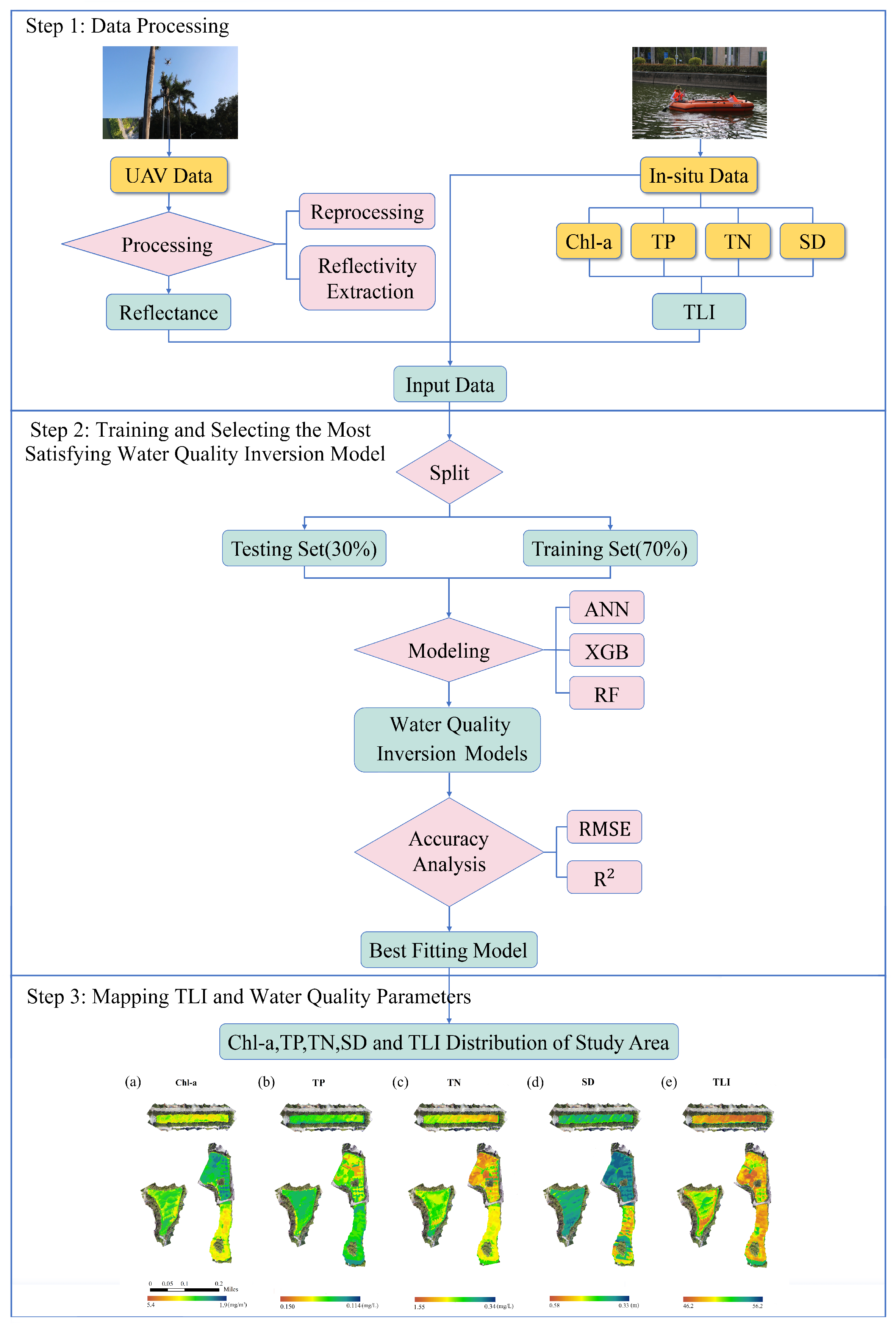
2.3.1. Data Processing

DJI Terra and The Environment for Visualizing Images (ENVI) were used to process the spectral data. As is shown in Figure 2, image preprocessing involving radiometric correction and image mosaic was completed by DJI Terra, a drone image processing software independently developed by DJI. As the flight height was low, errors caused by atmospheric radiation were excluded. Radiometric calibration was carried out by importing on-site photos of calibration plates taken before formal flights and the reflectivity data of the calibration plate in different bands as reference, by which the digital number value was converted to the radiance value by pixel.
After exporting the processed remote images, ENVI, a remote sensing image processing platform, was used to read the reflectivity of the five bands at 45 sampling points.

2.3.2. Quantification of Trophic State

The TLI is used to evaluate the trophic state of the lakes. Considering TN and TP are often limiting factors for algae in lakes and reservoirs, while SD and C O D M n are good reflection of algal biomass, Chinese scholars took the modified Carlson’s trophic state index ( T S I m ) [43] as reference and established TLI based on five water quality indicators, which are widely used in China [44,45]. The construction method was as follows: Nutritional levels were rated on a continuous scale from 0 to 100, with higher scores indicating higher levels of nutrition and associated risks. The index assumes that the corresponding TLI (Chl-a) is 0 and 100 when the Chl-a concentration is 0.1 and 1000 ug/L, respectively. Based on the hypothesis and the relationship between Chl-a and other chemical indicators of water quality (TN, TP, SD, C O D M n ), the evaluation equation of TLI and each water quality parameter are deduced as follows:
T L I Chl-a = 10 2.5 + 1.086 l n C h l a
T L I T P = 10 9.436 + 1.624 l n T P
T L I T N = 10 5.453 + 1.694 l n T N
T L I ( S D ) = 10 ( 5.118 1.94 l n S D )
T L I ( C O D M n ) = 10 ( 0.109 + 2.661 l n C O D M n )
T L I ( ) = j = 1 m W j · T L I ( j )
W j = r i j 2 j = 1 m r i j 2
where the unit of Chl-a is mg/ m 3 ; the units of TP, TN, and C O D M n are mg/L; and the unit of SD is meters. TLI(j), W j , and r i j represent the trophic state index, the weight coefficient and the correlation coefficient with the Chl-a of the j-th species parameter, respectively.
Based on the calculation results of the survey data of 26 major lakes in China, the correlation coefficients between Chl-a and each water quality parameter are obtained in Table 1:
Due to the lack of C O D M n data in our study area, T L I ( C O D M n ) is no longer included in the calculation of TLI. In this study, the expression for the TLI is:
T L I = 0.3261 T L I Chl-a + 0.2301 T L I T P + 0.2192 T L I T N + 0.2246 T L I ( S D )
The specific classifications are as follows: oligotrophic (TLI < 30), mesotrophic (30 ≤ TLI < 50), light eutrophic (50 ≤ TLI < 60), middle eutrophic (60 ≤ TLI < 70) and hyper eutrophic (TLI ≥ 70).

2.3.3. Modeling Approaches

(1) Water Quality Estimated Models
In this study, RF, XGB and ANN were chosen to build the inversion model of Chl-a, TP, TN, SD and TLI values, which are suitable for building black-box models between multiple factors that lack a significant physicochemical relationship. The reflectance of each point on 99 selected bands and band combinations was taken as the sample input, and the samples were divided into a training set (70%) and a testing set (30%), among which the former was used for model construction and the latter would be input to verify the accuracy of the models. Each parameter was modeled separately [46].
RF is an integrated algorithm combined by a number of Classification and Regression Trees (CART) [47]. As there were 99 input bands and band combinations, there were 99 characteristic values in the sample. After parameter adjustment, the number of CART in the RF model was set to 1000. Each CART in the model will extract a part of samples from the training set as a sub-training set, and a part of the 99 feature values will be randomly selected to find the optimal segmentation points to divide the left and right sub-CARTs. The final prediction result of this CART is the mean value of the leaf nodes reached by the sample points, and the final prediction result of RF model is the mean of the predicted value of all CARTs [48].
XGB is a gradient-boosting algorithm based on boosting trees. Compared with the traditional Gradient Boosting Decision Tree (GBDT), XGBR has a better anti-overfitting ability by adding the regularization into the loss function. Like RF, XGB also uses CART as a base regressor, uses a greedy algorithm to traverse all segmentation points of all features and finally takes the sum of all CARTs as the predicted value [49].
ANN is formed by a large number of interconnected processing units (neurons), including the input layer, hidden layer and output layer [50]. Due to the small amount of data in this study, only one hidden layer was used.
(2) Analysis of Model Accuracy and Correlation among Water Quality Indices
To find out the relationship and interaction between each water quality parameters and TLI, the Pearson correlation coefficient between any two parameters was calculated, measuring the linear correlation between two variables [51]. The higher the value is, the higher the correlation between the two indices. Meanwhile, the significance test was carried out to estimate the rationality of the coefficient. The significance level we used were 0.05, 0.01, 0.001, and in this order, the credibility of the hypothesis increases. The Pearson correlation coefficient is calculated as follows:
r = i = 1 n ( X i X ¯ ) ( Y i Y ¯ ) i = 1 n ( X i X ¯ ) 2 i = 1 n ( Y i Y ¯ ) 2
where X and Y are two group of parameters, and n is the number of samples.
The root mean square error (RMSE) and the coefficient of determination ( R 2 ) were selected to measure the accuracy of the models, which are defined as follows:
R M S E = 1 n i = 1 n ( y i f ( x i ) ) 2
R 2 = 1 i = 1 n ( y i f ( x i ) ) 2 i = 1 n ( y i y ¯ ) 2
where y is the measured value of each water quality parameter, and TLI, f ( x i ) is the predictive value; n is the number of samples.

3. Result

3.1. Measured Data Analysis and TLI Level

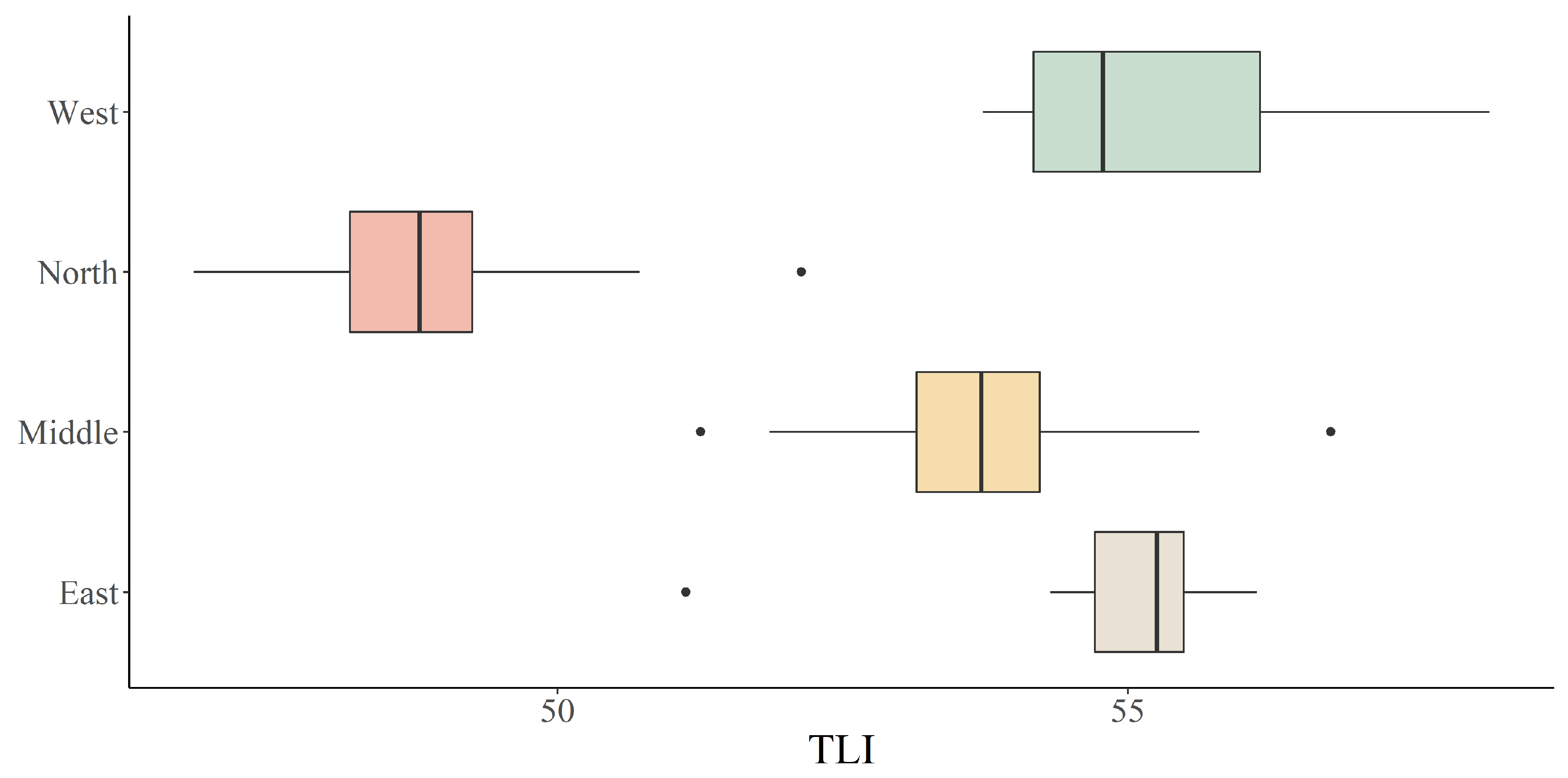
Observing the results in Figure 3, the TLI of our study area varied gently between different samples and was totally at a low level, ranging from 46.81 to 58.17, which showed that the lakes were in a mesotrophic or a light eutrophic state. From Figure 3, it was obvious that the trophic level of North Lake was significantly lower than the other three lakes with the average TLI of under 50, while that of the other three lakes was above 54, which showed the geographical heterogeneity of TLI, as the three lakes are close to each other, while North Lake is about 1.3 km away from them. This was also in line with our field observation results. During sampling, we found that compared with the other three lakes, the shore of the North Lake has significantly more aquatic animals and plants, showing a better ecological environment.
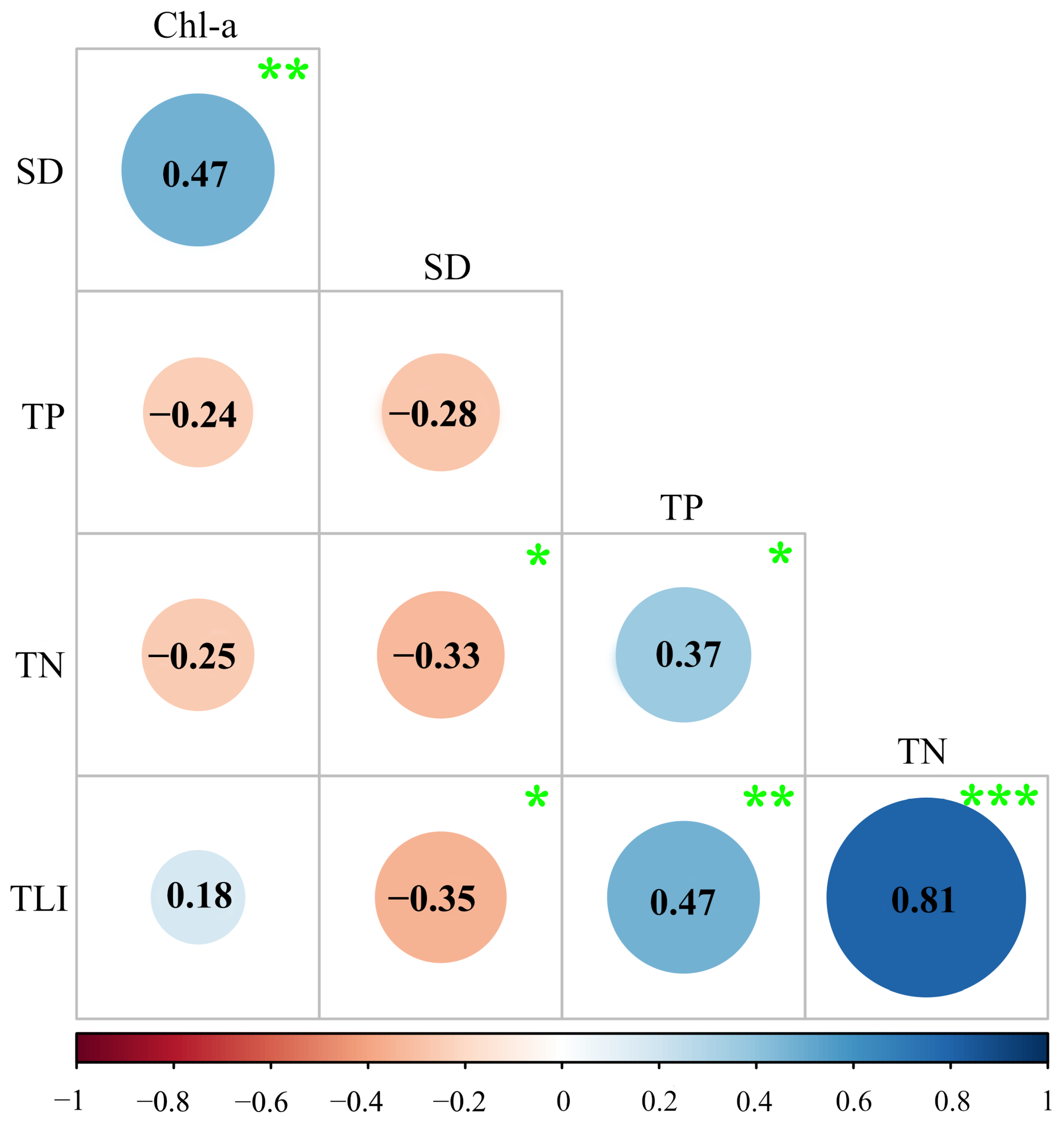
To find the relationship between the water quality parameters and TLI in our study area, the Pearson correlation coefficients between them were calculated, shown in Figure 4. Within four water quality parameters, TN displayed the most significant correlation with TLI with a correlation coefficient of 0.81 at the 0.001 significance level. Besides, compared to several other water quality parameters that varied in a very narrow range, spans of TN were also the largest. According to the Environmental Quality Standards for Surface Water (GB3838-2002), the TN in our study area spanned 0.153 to 1.88, covering class I to V, which may result in the strong correlation between TLI and TN. As the limiting factor of eutrophication, TP also had a strong positive correlation with TLI, while transparency had a weak negative correlation with the above three factors, which is because the water under eutrophication will become muddy and reduce the ornamental value. Surprisingly, Chl-a, the core parameter in TLI construction, had a low correlation coefficient with TLI (only 0.18), which was contrary to our expectation. The reason was speculated to be the small variation and overall low level of Chl-a in our study area.

3.2. Model Accuracy Verification and Comparison

RF, XGB and ANN were used to construct inversion models, respectively. All three models were optimized to ensure that relatively accurate results were obtained. The evaluation accuracy of each model is shown in Table 2.
It is found that the three regression models showed a certain consistency in the estimation precision of each index, that is, among the five parameters, TN had the highest accuracy and average determination coefficient ( R 2 = 0.89 , R M S E = 0.24 ) . The photosensitive Chl-a and the observable SD followed with R 2 of 0.81 and 0.82, respectively, showing good performance. On the contrary, the fitting effect of TP is poor, for the R 2 of the three models is no more than 0.7.
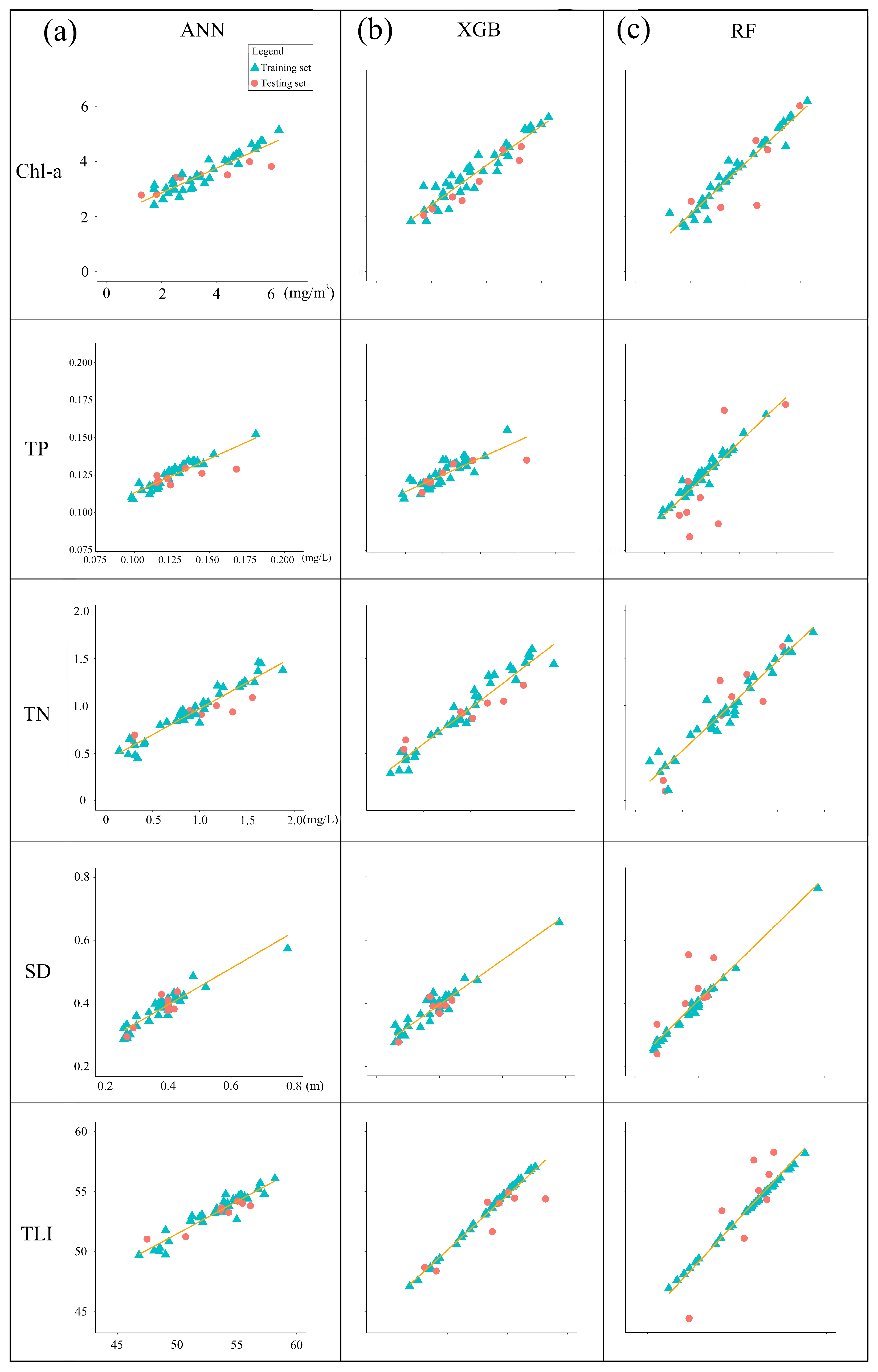
Considering Figure 5, it can be observed that, although there is no significant gap between RF and the other two algorithms in terms of R 2 and RMSE, the tropic line of RF deviates from the line of 45 degrees in the scatter plots, which proves that the predicted values are not in good agreement with measured values, leading to the loss of the credibility of the RF models. Among the remaining two models, ANN performed better at estimating Chl-a and TP because the regression line is near 45 degrees. The opposite is true for the other three parameters, with XGB performing better. Combined with the consideration of R 2 a n d R M S E in Table 2, XGB outperformed ANN with the best average accuracy validation metrics ( R 2 = 0.83 , R M S E = 0.52 ) . Therefore, we can deduce that the XGB model is the most suitable for water-quality inversion among the three models mentioned above.

3.3. Spatial Distribution of Water Quality and Eutrophication Degree

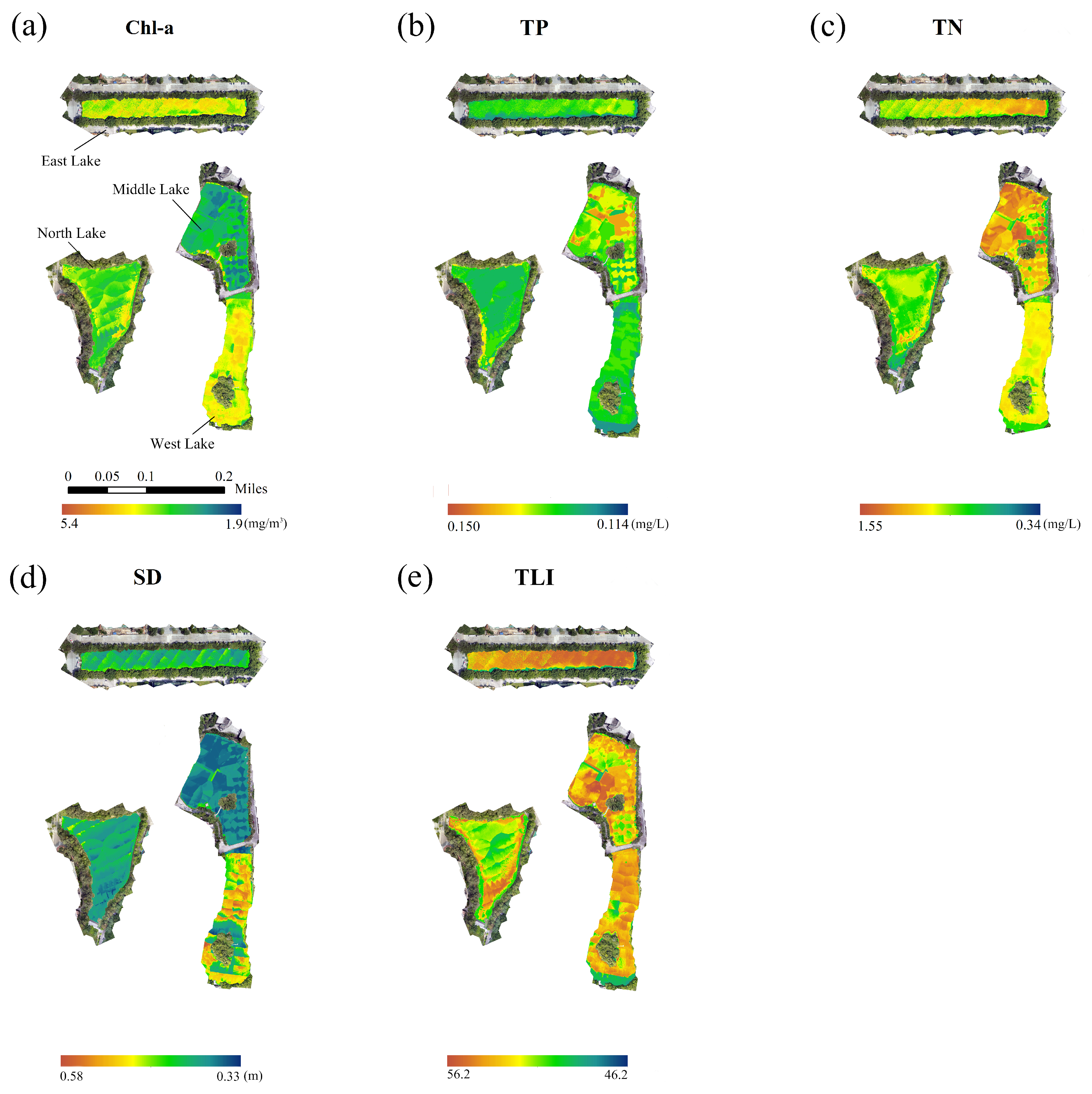
Based on the above results, the XGB model was confirmed as the optimal inversion model with the highest accuracy and was used to retrieve the water quality parameters in the study area to draw the distribution map (Figure 6). The region with the size of 5*5 pixels on the remote sensing image was taken as the unit for cyclic extraction, and the average reflectance value of all 25 pixels was taken as the input variable of the region.
The spatial distribution of TLI is consistent with our expectation based on the measured data, with little overall change. The TLI values in most areas remain in the light eutropher state, while a small part is in the mesotropher state. From the perspective of distribution span, the range of TN is the largest, which is also in good agreement with the measured data. As the water quality parameter with the strongest correlation with TLI, its distribution is almost consistent with TLI, that is, the indices of North Lake are significantly lower than those of the other three lakes. The distribution of TP is relatively uniform, concentrated around 0.13. Only in some areas of Middle Lake did it increase significantly, which may be related to the distribution of the drainage outlet. The values of Chl-a in North Lake and Middle Lake are lower than those in West Lake and East Lake, and there is an obvious upward trend from Middle Lake to West Lake.
It is worth noting that we deliberately included the part covered by shadows in the selection of water areas. It can be seen that, except SD and Chl-a, the other three indicators are significantly different between the shaded area and the non-shaded area, and the values of the shaded area are all lower than normal. Taking the distribution of TP as an example, the TP values in the shaded area on the right bank of East Lake and the lower side of West Lake are obviously lower than the surrounding normal values, and the blue–green boundary on the distribution map is the shaded boundary, which allows us to confirm that shading does have a significant impact on the analysis of multispectral data.
Overall, based on the analysis of TLI values in our study area, we believe that the current trophic status of the lakes is relatively normal and that there is no hyper eutrophication risk.

4. Discussion

From the result, the three algorithms (RF, XGB, ANN) we adopted in this study all showed high R 2 , which shows that the black-box model based on artificial intelligence algorithm is suitable for the data without obvious physical mechanism. Wei et al. used several artificial intelligence algorithms to identify black-odor water bodies in cities and gained results with higher reliability [52], which is consistent with our results. Among the three models, XGB performs the best, which is thought to be related to its innovation in error reduction and noise processing. As a new boosting algorithm, XGB makes a lot of improvements on the basis of GBDT. One of the most important optimizations is the addition of a regularized model to reduce overfitting, which greatly improves the generalization ability of the model [49]. Therefore, compared with RF, which is prone to overfitting when dealing with noisy data [53], the results of XGB models are more accurate in this study. As one of the earliest developed machine learning algorithms, ANN is also the first to be applied in the study of water-quality inversion using empirical methods [50]. The limited sample size in our study may not show its advantages. However, in recent years, deep learning methods evolved from ANN, such as cyclic and convolutional neural networks, still have a huge space for development and exploration in the application of water-quality remote sensing [35].
By analyzing the water surface morphology of East Lake through visible-light photos, it is found that there is sun glint distributed on the lake, which is due to the specular reflection phenomenon caused by waves and the specific solar height angle. Studies have shown that the reflectivity of all bands in sun glint region increases in different amplitudes according to the shape and size of the wave [54]. In this study, due to the small impact scope and not covering the sample point, the sun glint does not affect the process of modeling. However, when analyzing the TLI distribution of the study area subsequently, the area covered by light plot showed a difference from other areas, reflected in the pixel units with obvious color difference from the surrounding areas. In order to reduce the effect of mirror reflection, we have to avoid a period of high solar elevation angle when choosing 8–10 a.m. and 2–4 p.m. to collect spectral data. In future studies, attention should be paid to the solar altitude angle and water surface condition when sampling.
In the TLI inversion of the study area, we used the remote sensing images of the day for collecting data to extract the reflectivity and did not deliberately avoid the shadow part. The results shows that the three parameters, TLI, TN and TP, were significantly reduced in the shaded area and generated an obvious dividing line. The shadow will express the spectral characteristics of the water body, so that the amount of radiation is reduced [55,56], thereby obtaining an index below normal. However, there is no significant abnormality in the predicted values of Chl-a and SD in the shaded area. We speculated that the former is the only visible physical index, while the latter is photosensitive with the obvious absorption effect in the red band. The relationship between them and the spectral information is more significant than the other parameters, which may have been the reason why they have a better anti-shadow interference property. Clearly, further work is required to confirm it. At present, the research about the influence of shadows on water remote sensing is mainly aimed at weakening the influence of cloud shadow on ocean water inversion [56]. The compensation method of urban water-quality inversion affected by ground object shadow based on high-resolution remote sensing is relatively blank.
In addition, we find that the prediction results of the XGB model are relatively conservative. Some extreme values that are significantly different from the overall trend have not been accurately estimated compared to the true values. For example, the maximum measured value of SD (0.78) is 39.3% higher than the sub-maximum value (0.56). However, the maximum value of the inversion results is 0.58, which is closer to the sub-maximum value, so we speculate that it does not support the extreme case wherein the prediction deviates from the overall trend significantly. Therefore, after removing the maximum and minimum values, the inversion accuracy of the model will be improved. However, it is worth noting that, among the five parameter inversions, the results of TLI are least affected by this condition. In future model training, it is suggested to measure the degree to which the extreme value influences the trend line and the estimation of fitted value and then to process the raw data to reduce this effect.
In this study, we used TLI to quantify the trophic state, which takes Chl-a as the benchmark weight and determines the weights of other water quality parameters through the correlation between Chl-a and them, respectively. When constructing TLI expression, we used correlation data from the survey of 26 lakes in China to calculate each weight. However, through the correlation analysis of each water quality parameter in our field sampling results, we found that it was different from the statistical data we used, which would affect the contribution of each parameter to the degree of nutrition, leading to some errors. In order to avoid such errors, the weights of water quality parameters in TLI should be recalculated in different study areas.
According to the Action Plan for Prevention and Control of Water Pollution in 2015, Guangzhou city enacted efforts in water-environment treatment by carrying out a series of measures to maintain the nutrient-rich water body at a good level. From the environmental Quality Status Report of Guangzhou in 2021, the water quality in the study area is all class II. When sampling, we found that the TLI values at all points did not exceed 60, that is, all the sampling points did not reach the middle eutropher state, which has a certain negative impact on the establishment of the model. Due to the lack of spectral data of middle or above eutrophic water, we cannot guarantee the accuracy of the model in the prediction of water bodies with TLI < 30 or > 60. Zhu and Mao found a similar situation for the lack of non-eutrophic samples in modeling [39].
According to the study, we believe that, as an emerging artificial intelligence algorithm, XGB is optimal for building an inversion model of water quality with a small sample, which shows an excellent fitting effect and is recommended to use. In future research, we suggest that more attention should be paid to the influence and interference of mirror reflection and shadow on multispectral data. In addition, water bodies with a wider range of water quality should be selected as research objects to obtain models with good prediction effects for various trophic states.

5. Conclusions

In this study, we sampled and tested 45 points in the study area, used three algorithms to retrieve the trophic state and then selected the optimal model to draw the spatial distribution map of water quality, resulting in the following conclusions:
(1) North, West, East and Middle Lakes of SCUT were selected for data collection in clear weather. The spectral data of UAV and water quality data were collected simultaneously. By analyzing the water quality parameters at each point, we found that the water quality in the study area was relatively stable. The overall levels of Chl-a, TP and SD were low. TN, on the other hand, has a certain spatial specificity, with a maximum value of 1.88, belonging to Class Ⅴ. Since TN is one of the limiting factors of eutrophication, the water quality monitoring of water discharged into this area should be strengthened to avoid eutrophication risk.
(2) Due to the active implementation of water control policies in Guangzhou, the water quality in our study area is good, with a mesotrophic or light eutrophic state. Among the four lakes, North Lake has the lowest TLI, which is basically in the mesotrophic state. Through field observation, its ecological environment, biodiversity and ornamental value are also the best.
(3) Judging from the accuracy evaluation results of the RF, ANN and XGB models, the validation indices of the three models are all satisfactory. As a new algorithm, XGB performs best for water-quality inversion in this area ( R 2 = 0.83, RMSE = 0.52). The model was used to invert the water quality and draw the spatial distribution map. The results of the map are in good agreement with the measured ones, so that we confirm that XGB is well suited for water-quality inversion.
In future work, it is encouraged to (1) use a wider range of data to train the model and thus develop high-precision inversion models suitable for water bodies of all trophic levels, (2) take the influence of specular reflection and ground object shadow into account to develop an appropriate compensation formula to reduce the environmental error and (3) explore the possibility of the latest algorithms such as deep learning in the field of urban water-quality inversion.

Author Contributions

D.W.: writing—original draft and editing, field investigation, laboratory analyses, program running; J.J.: conceptualization, writing—review and editing, field investigation, laboratory analyses; F.W.: writing—editing, field investigation, laboratory analyses; Y.L.: writing—editing, field investigation, laboratory analyses.; X.L.: writing—editing, field investigation, laboratory analyses.; C.L.: conceptualization, writing—review and editing, supervision; X.W.: data curation and validation, writing—review and editing, supervision; M.X.: resources, project administration, supervision. All authors have read and agreed to the published version of the manuscript.

Funding

The research is financially supported by the National Key R&D Program of China (2021YFC3001000), the National Natural Science Foundation of China (52109019, 51879107, U1911204) and the Science and Technology Planning Project of Guangdong Province in China (2020A0505100009).

Data Availability Statement

The authors confirm that the data supporting the findings of this study are available within the article (in Appendix A).

Acknowledgments

We appreciate all the authors who contributed to the work and participated in the fieldwork and laboratory analyses.

Conflicts of Interest

The authors declare no conflict of interest.

Appendix A

Table A1. Measured water quality parameters of each sampling point.
Sampling PointChl-aTPTNSD
( m g / m 3 ) ( m g / L ) ( m g / L ) ( m )
14.620.1390.4210.4
24.60.1030.2620.42
34.390.1050.1520.43
43.010.0990.3150.38
53.560.0980.2460.44
62.540.1250.3150.4
72.240.110.3450.39
83.40.1150.2960.4
92.770.1460.3180.3
102.460.1220.410.4
112.430.1410.5830.4
125.40.1160.8990.45
135.990.110.9120.42
145.270.1420.8230.4
155.670.1151.050.42
163.280.1251.450.37
172.160.1531.880.38
184.720.1391.210.4
195.20.130.8650.78
203.710.1230.9550.38
215.480.1240.8350.52
226.260.1161.090.34
232.740.1151.020.36
244.790.12210.4
253.30.1810.6540.37
264.820.1170.8960.48
273.420.1171.050.37
284.30.1121.350.38
292.390.1160.9560.43
301.740.1141.180.45
312.690.1360.9550.4
324.430.1110.7560.42
335.610.1160.8150.43
341.820.141.560.4
351.720.1341.480.26
363.880.1391.420.3
372.640.1331.650.26
383.050.1451.040.27
393.740.1230.80.28
402.060.1271.250.27
413.120.1681.620.27
423.050.130.8020.29
431.260.1321.620.27
442.040.121.580.34
451.730.1271.190.27

References

  1. Smith, V.H.; Schindler, D.W. Eutrophication science: Where do we go from here? Trends Ecol. Evol. 2009, 24, 201–207. [Google Scholar] [CrossRef]
  2. Matthews, M.W.; Bernard, S. Eutrophication and cyanobacteria in South Africa’s standing water bodies: A view from space. S. Afr. J. Sci. 2015, 111, 7. [Google Scholar] [CrossRef] [Green Version]
  3. Smith, V.H.; Joye, S.B.; Howarth, R.W. Eutrophication of freshwater and marine ecosystems. Limnol. Oceanogr. 2006, 51, 351–355. [Google Scholar] [CrossRef] [Green Version]
  4. Nazari-Sharabian, M.; Taheriyoun, M. Climate change impact on water quality in the integrated Mahabad Dam watershed-reservoir system. J. Hydro Environ. Res. 2021, 40, 28–37. [Google Scholar] [CrossRef]
  5. Guan, Q.; Feng, L.; Hou, X.; Schurgers, G.; Zheng, Y.; Tang, J. Eutrophication changes in fifty large lakes on the Yangtze Plain of China derived from MERIS and OLCI observations. Remote Sens. Environ. 2020, 246, 111890. [Google Scholar] [CrossRef]
  6. Ke, S.; Zhang, P.; Ou, S.; Zhang, J.; Chen, J.; Zhang, J. Spatiotemporal nutrient patterns, composition, and implications for eutrophication mitigation in the Pearl River Estuary, China. Estuar. Coast. Shelf Sci. 2022, 266, 107749. [Google Scholar] [CrossRef]
  7. Huang, X.; Huang, L.; Yue, W. The characteristics of nutrients and eutrophication in the Pearl River estuary, South China. Mar. Pollut. Bull. 2003, 47, 30–36. [Google Scholar] [CrossRef]
  8. Ministry of Ecology and Environment. China Ecological and Environmental Bulletin 2019; Ministry of Ecology and Environment in China, 15 December 2019. Available online: https://www.mee.gov.cn/xxgk2018/xxgk/xxgk15/202005/t20200507_777895.html (accessed on 7 May 2020). (In Chinese)
  9. Schindler, D.W. Recent advances in the understanding and management of eutrophication. Limnol. Oceanogr. 2006, 51, 356–363. [Google Scholar] [CrossRef] [Green Version]
  10. Yang, Y.; Bai, Y.; Wang, X.; Wang, L.; Jin, X.; Sun, Q. Group Decision-Making Support for Sustainable Governance of Algal Bloom in Urban Lakes. Sustainability 2020, 12, 1494. [Google Scholar] [CrossRef] [Green Version]
  11. Sharabian, M.N.; Ahmad, S.; Karakouzian, M. Climate Change and Eutrophication: A Short Review. Eng. Technol. Appl. Sci. Res. 2018, 8, 3668–3672. [Google Scholar] [CrossRef]
  12. Gholizadeh, M.H.; Melesse, A.M.; Reddi, L. A Comprehensive Review on Water Quality Parameters Estimation Using Remote Sensing Techniques. Sensors 2016, 16, 1298. [Google Scholar] [CrossRef] [PubMed] [Green Version]
  13. Verma, S. Wireless Sensor Network Application for Water Quality Monitoring in India. In Proceedings of the 2012 National Conference on Computing and Communication Systems, Durgapur, India, 21–22 November 2012; IEEE: Piscataway, NJ, USA, 2012; pp. 1–5. [Google Scholar]
  14. Adu-Manu, K.S.; Katsriku, F.A.; Abdulai, J.-D.; Engmann, F. Smart River Monitoring Using Wireless Sensor Networks. Wirel. Commun. Mob. Comput. 2020, 2020, 1–19. [Google Scholar] [CrossRef]
  15. Park, J.; Kim, K.T.; Lee, W.H. Recent Advances in Information and Communications Technology (ICT) and Sensor Technology for Monitoring Water Quality. Water 2020, 12, 510. [Google Scholar] [CrossRef] [Green Version]
  16. Robarts, R.D.; Barker, S.J.; Evans, S. Water Quality Monitoring and Assessment: Current Status and Future Needs. In Proceedings of the 12th World Lake Conference, Jaipur, Rajasthan, India, 28 October–2 November 2007. [Google Scholar]
  17. Cheng, K.-S.; Lei, T.-C. Reservoir Trophic State Evaluation Using Lanisat Tm Images. JAWRA J. Am. Water Resour. Assoc. 2001, 37, 1321–1334. [Google Scholar] [CrossRef]
  18. Mamun, M.; Ferdous, J.; An, K.-G. Empirical Estimation of Nutrient, Organic Matter and Algal Chlorophyll in a Drinking Water Reservoir Using Landsat 5 TM Data. Remote Sens. 2021, 13, 2256. [Google Scholar] [CrossRef]
  19. Shi, J.; Shen, Q.; Yao, Y.; Li, J.; Chen, F.; Wang, R.; Xu, W.; Gao, Z.; Wang, L.; Zhou, Y. Estimation of Chlorophyll-a Concentrations in Small Water Bodies: Comparison of Fused Gaofen-6 and Sentinel-2 Sensors. Remote Sens. 2022, 14, 229. [Google Scholar] [CrossRef]
  20. Soomets, T.; Uudeberg, K.; Jakovels, D.; Brauns, A.; Zagars, M.; Kutser, T. Validation and Comparison of Water Quality Products in Baltic Lakes Using Sentinel-2 MSI and Sentinel-3 OLCI Data. Sensors 2020, 20, 742. [Google Scholar] [CrossRef] [Green Version]
  21. Cao, Z.; Ma, R.; Duan, H.; Pahlevan, N.; Melack, J.; Shen, M.; Xue, K. A machine learning approach to estimate chlorophyll-a from Landsat-8 measurements in inland lakes. Remote Sens. Environ. 2020, 248, 111974. [Google Scholar] [CrossRef]
  22. Zhang, T.; Huang, M.; Wang, Z. Estimation of chlorophyll-a Concentration of lakes based on SVM algorithm and Landsat 8 OLI images. Environ. Sci. Pollut. Res. 2020, 27, 14977–14990. [Google Scholar] [CrossRef]
  23. Moses, W.J.; Gitelson, A.A.; Berdnikov, S.; Povazhnyy, V. Satellite Estimation of Chlorophyll-a Concentration Using the Red and NIR Bands of MERIS—The Azov Sea Case Study. IEEE Geosci. Remote. Sens. Lett. 2009, 6, 845–849. [Google Scholar] [CrossRef]
  24. Palmer, S.C.J.; Kutser, T.; Hunter, P.D. Remote sensing of inland waters: Challenges, progress and future directions. Remote Sens. Environ. 2015, 157, 1–8. [Google Scholar] [CrossRef] [Green Version]
  25. Gitelson, A.; Garbuzov, G.; Szilagyi, F.; Mittenzwey, K.-H.; Karnieli, A.; Kaiser, A. Quantitative remote sensing methods for real-time monitoring of inland waters quality. Int. J. Remote. Sens. 1993, 14, 1269–1295. [Google Scholar] [CrossRef]
  26. Aasen, H.; Honkavaara, E.; Lucieer, A.; Zarco-Tejada, P.J. Quantitative Remote Sensing at Ultra-High Resolution with UAV Spectroscopy: A Review of Sensor Technology, Measurement Procedures, and Data Correction Workflows. Remote Sens. 2018, 10, 1091. [Google Scholar] [CrossRef] [Green Version]
  27. Olivetti, D.; Roig, H.; Martinez, J.-M.; Borges, H.; Ferreira, A.; Casari, R.; Salles, L.; Malta, E. Low-Cost Unmanned Aerial Multispectral Imagery for Siltation Monitoring in Reservoirs. Remote Sens. 2020, 12, 1855. [Google Scholar] [CrossRef]
  28. Pasler, M.; Komarkova, J.; Sedlak, P. Comparison of possibilities of UAV and Landsat in observation of small inland water bodies. In Proceedings of the 2015 International Conference on Information Society (i-Society), London, UK, 9–11 November 2015; pp. 45–49. [Google Scholar] [CrossRef]
  29. Gilerson, A.A.; Huot, Y. Chapter 7—Bio-optical Modeling of Sun-Induced Chlorophyll-a Fluorescence. In Bio-Optical Modeling and Remote Sensing of Inland Waters; Mishra, D.R., Ogashawara, I., Gitelson, A.A., Eds.; Elsevier: Amsterdam, The Netherlands, 2017; pp. 189–231. ISBN 978-0-12-804644-9. [Google Scholar]
  30. Dörnhöfer, K.; Oppelt, N. Remote sensing for lake research and monitoring–Recent advances. Ecol. Indic. 2016, 64, 105–122. [Google Scholar] [CrossRef]
  31. Kutser, T.; Metsamaa, L.; Strömbeck, N.; Vahtmäe, E. Monitoring cyanobacterial blooms by satellite remote sensing. Estuar. Coast. Shelf Sci. 2006, 67, 303–312. [Google Scholar] [CrossRef]
  32. Lee, Z.; Carder, K.L.; Arnone, R.A. Deriving inherent optical properties from water color: A multiband quasi-analytical algorithm for optically deep waters. Appl. Opt. 2002, 41, 5755–5772. [Google Scholar] [CrossRef]
  33. Li, L.; Li, L.; Song, K.; Li, Y.; Tedesco, L.P.; Shi, K.; Li, Z. An inversion model for deriving inherent optical properties of inland waters: Establishment, validation and application. Remote Sens. Environ. 2013, 135, 150–166. [Google Scholar] [CrossRef]
  34. Bricaud, A.; Babin, M.; Morel, A.; Claustre, H. Variability in the chlorophyll-specific absorption coefficients of natural phytoplankton: Analysis and parameterization. J. Geophys. Res. Atmos. 1995, 100, 13321–13332. [Google Scholar] [CrossRef]
  35. Sagan, V.; Peterson, K.T.; Maimaitijiang, M.; Sidike, P.; Sloan, J.; Greeling, B.A.; Maalouf, S.; Adams, C. Monitoring inland water quality using remote sensing: Potential and limitations of spectral indices, bio-optical simulations, machine learning, and cloud computing. Earth Sci. Rev. 2020, 205, 103187. [Google Scholar] [CrossRef]
  36. Allan, M.G.; Hamilton, D.P.; Hicks, B.; Brabyn, L. Empirical and semi-analytical chlorophyll a algorithms for multi-temporal monitoring of New Zealand lakes using Landsat. Environ. Monit. Assess. 2015, 187, 1–24. [Google Scholar] [CrossRef] [PubMed]
  37. Kageyama, Y.; Takahashi, J.; Nishida, M.; Kobori, B.; Nagamoto, D. Analysis of water quality in Miharu dam reservoir, Japan, using UAV data. IEEJ Trans. Electr. Electron. Eng. 2016, 11, S183–S185. [Google Scholar] [CrossRef]
  38. Peterson, K.T.; Sagan, V.; Sidike, P.; Cox, A.L.; Martinez, M. Suspended Sediment Concentration Estimation from Landsat Imagery along the Lower Missouri and Middle Mississippi Rivers Using an Extreme Learning Machine. Remote Sens. 2018, 10, 1503. [Google Scholar] [CrossRef] [Green Version]
  39. Zhu, S.; Mao, J. A Machine Learning Approach for Estimating the Trophic State of Urban Waters Based on Remote Sensing and Environmental Factors. Remote Sens. 2021, 13, 2498. [Google Scholar] [CrossRef]
  40. Lim, J.; Choi, M. Assessment of Water Quality Based on Landsat 8 Operational Land Imager Associated with Human Activities in Korea. Environ. Monit. Assess. 2015, 187, 1–17. [Google Scholar] [CrossRef]
  41. Carlson, R.E. A trophic state index for lakes. Limnol. Oceanogr. 1977, 22, 361–369. [Google Scholar] [CrossRef] [Green Version]
  42. Nazari-Sharabian, M.; Taheriyoun, M.; Ahmad, S.; Karakouzian, M.; Ahmadi, A. Water Quality Modeling of Mahabad Dam Watershed–Reservoir System under Climate Change Conditions, Using SWAT and System Dynamics. Water 2019, 11, 394. [Google Scholar] [CrossRef] [Green Version]
  43. Aizaki, M.; Otsuki, A.; Fukushima, T.; Hosomi, M.; Muraoka, K. Application of Carlson’s trophic state index to Japanese lakes and relationships between the index and other parameters. SIL Proc. 1922–2010 1981, 21, 675–681. [Google Scholar] [CrossRef]
  44. Wei, Z.; Guangwei, Z.; Yongjiu, C.; Hai, X.; Mengyuan, Z.; Zhijun, G.; Yunlin, Z.; Boqiang, Q. The limitations of comprehensive trophic level index (TLI) in the eutrophication assessment of lakes along the middle and lower reaches of the Yangtze River during summer season and recommendation for its improvement. J. Lake Sci. 2020, 32, 36–47. [Google Scholar] [CrossRef]
  45. Wang, M.; Liu, X.; Zhang, J. Evaluate Method and Classification Standard on Lake Eutrophication. Environ. Monit. China 2002, 18, 47–49. (In Chinese) [Google Scholar] [CrossRef]
  46. Wu, X.; Wang, Z.; Guo, S.; Liao, W.; Zeng, Z.; Chen, X. Scenario-based projections of future urban inundation within a coupled hydrodynamic model framework: A case study in Dongguan City, China. J. Hydrol. 2017, 547, 428–442. [Google Scholar] [CrossRef]
  47. Li, J.; Wang, Z.; Wu, X.; Xu, C.; Guo, S.; Chen, X.; Zhang, Z. Robust Meteorological Drought Prediction Using Antecedent SST Fluctuations and Machine Learning. Water Resour. Res. 2021, 57. [Google Scholar] [CrossRef]
  48. Breiman, L. Random Forest. Mach. Learn. 2001, 45, 5–32. [Google Scholar] [CrossRef] [Green Version]
  49. Chen, T.; Guestrin, C. XGBoost: A Scalable Tree Boosting System. In Proceedings of the 22nd ACM SIGKDD International Conference on Knowledge Discovery and Data Mining, San Francisco, CA, USA, 13 August 2016; ACM: New York, NY, USA; pp. 785–794. [Google Scholar]
  50. Maier, H.R.; Jain, A.; Dandy, G.C.; Sudheer, K. Methods used for the development of neural networks for the prediction of water resource variables in river systems: Current status and future directions. Environ. Model. Softw. 2010, 25, 891–909. [Google Scholar] [CrossRef]
  51. Li, J.; Wang, Z.; Wu, X.; Zscheischler, J.; Guo, S.; Chen, X. A standardized index for assessing sub-monthly compound dry and hot conditions with application in China. Hydrol. Earth Syst. Sci. 2021, 25, 1587–1601. [Google Scholar] [CrossRef]
  52. Wei, L.; Huang, C.; Wang, Z.; Zhou, X.; Cao, L. Monitoring of Urban Black-Odor Water Based on Nemerow Index and Gradient Boosting Decision Tree Regression Using UAV-Borne Hyperspectral Imagery. Remote Sens. 2019, 11, 2402. [Google Scholar] [CrossRef] [Green Version]
  53. Segal, M.R. Machine Learning Benchmarks and Random Forest Regression; UCSF: Center for Bioinformatics and Molecular Biostatistics: San Francisco, CA, USA.
  54. Zeng, C.; Richardson, M.; King, D.J. The impacts of environmental variables on water reflectance measured using a lightweight unmanned aerial vehicle (UAV)-based spectrometer system. ISPRS J. Photogramm. Remote. Sens. 2017, 130, 217–230. [Google Scholar] [CrossRef]
  55. Wójcik-Długoborska, K.; Bialik, R. The Influence of Shadow Effects on the Spectral Characteristics of Glacial Meltwater. Remote Sens. 2020, 13, 36. [Google Scholar] [CrossRef]
  56. Mostafa, Y.; Abdelhafiz, A. Shadow Identification in High Resolution Satellite Images in the Presence of Water Regions. Photog ramm. Eng. Remote. Sens. 2017, 83, 87–94. [Google Scholar] [CrossRef]
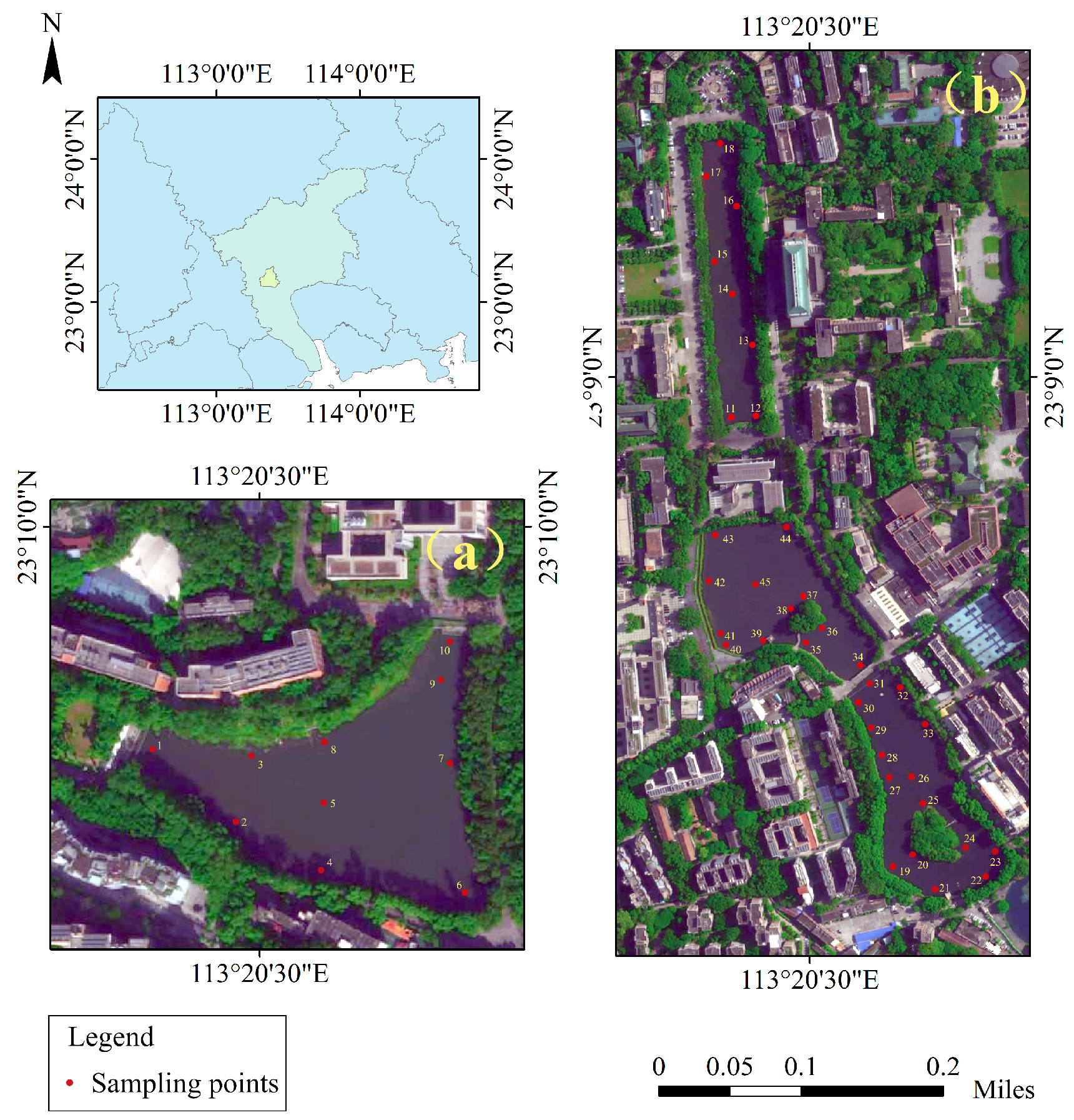
Figure 1. Location of the study area and the distribution of sampling sites. (a) North Lake, (b) East Lake, Middle Lake and West Lake (from top to bottom).
Water 15 00354 g001
Figure 2. Workflow for image processing, data analysis and modeling. Spatial distribution of different water quality parameters based on the XGB model in step 3: (a) Chl-a, (b) TP, (c) TN, (d) SD, (e) TLI.
Water 15 00354 g002
Figure 3. TLI distribution of four lakes in the study area.
Water 15 00354 g003
Figure 4. Correlation among water quality indices (green ***, ** and * mean significant correlation at the 0.001, 0.01 and 0.05 levels; the number in the circle refers to Pearson correlation coefficient).
Water 15 00354 g004
Figure 5. The scatter plots for the predicted and in situ values of each water quality parameter based on the following models: (a) RF, (b) XGB, (c) ANN.
Water 15 00354 g005
Figure 6. Spatial distribution of different water quality parameters based on the XGB model: (a) Chl-a, (b) TP, (c) TN, (d) SD, (e) TLI.
Water 15 00354 g006
Table 1. r i j and r i j 2 values between some parameters and Chl-a in Chinese lakes.
IndicatorsChl-aTPTNSD C O D M n
r i j 10.840.82−0.830.83
r i j 2 10.70560.67240.68890.6889
Table 2. Accuracy validation metrics of different regression models.
Chl-aTPTNSDTLI
R 2 RMSE R 2 RMSE R 2 RMSE R 2 RMSE R 2 RMSE
RF0.811.200.490.020.880.290.910.030.881.67
XGB0.930.580.670.020.950.230.810.030.811.64
ANN0.701.510.590.020.850.200.740.090.782.47
Disclaimer/Publisher’s Note: The statements, opinions and data contained in all publications are solely those of the individual author(s) and contributor(s) and not of MDPI and/or the editor(s). MDPI and/or the editor(s) disclaim responsibility for any injury to people or property resulting from any ideas, methods, instructions or products referred to in the content.