Article

A Multi-Objective Decision Model for Water Pollution Load Allocation under Uncertainty

1
School of Chemical and Environmental Engineering, Anhui Polytechnic University, Wuhu 241000, China
2
School of Civil Engineering, Anhui Polytechnic University, Wuhu 241000, China
*
Author to whom correspondence should be addressed.
Water 2023, 15(2), 309; https://doi.org/10.3390/w15020309
Submission received: 29 November 2022 / Revised: 7 January 2023 / Accepted: 9 January 2023 / Published: 11 January 2023
(This article belongs to the Special Issue Integrated Water Resources Modeling and Management)

Abstract

:
In order to control the discharge of regional total pollutants in the region and improve the ability of water environment management and decision making, a multi-objective decision-making optimization model of water pollution load allocation was constructed, which took into account economy and fairness. The model takes the maximum environmental benefit and the minimum weighted comprehensive Gini coefficient as the objective function and takes into account the uncertainty and multi-objectives of the model, which is conducive to promoting economic development and ensuring the fairness of regional water pollutant discharge. A method based on Monte Carlo simulation coupled with a genetic algorithm was designed to obtain the optimal solution set through multiple simulation optimization. This model is applied to Anhui Province to solve the allocation optimization problem of total pollutant reduction in the 13th Five-Year Energy Conservation and Emission Reduction Plan. After the optimization of water pollution load distribution, the comprehensive Gini coefficients of COD and NH3-N are reduced by different ranges. The comprehensive Gini coefficient after COD optimization decreased by 2.4–4.6%, and the comprehensive Gini coefficient after NH3-N optimization decreased by 25.1–32.5%, which verified the feasibility and rationality of the model in the optimal allocation of the total discharge of regional water pollutants. The model takes into account uncertain subjective and objective factors that have an important impact on water pollutant discharge targets and decision variables, thus optimizing the total emissions of the entire regional control unit in both space and time.

1. Introduction

With the rapid expansion of population and related economic activities and urbanization, the contradiction of water shortage caused by water quality has become a bottleneck restricting regional economic development [1,2]. In recent years, with the “13th Five-Year Plan” energy conservation and emission reduction plans proposed by various provinces and cities, the total amount of pollutant control has gradually become the main method of water environment planning and management [3,4]. Therefore, how to distribute the pollution load fairly and effectively is crucial to controlling the total amount of pollutants [5,6,7].
Fairness and efficiency are the two basic decision-making principles for pollution load distribution [8], which can be defined by the Gini coefficient. The Gini coefficient is an index that comprehensively examines the difference in income distribution between economic and social residents in economics. It was first proposed by Italian economist Gini in the early 20th century. The lower the Gini coefficient, the higher the fairness and efficiency of social distribution; on the contrary, the lower the fairness and efficiency, the higher the Gini coefficient. Previous studies have often taken “efficiency first, taking into account fairness” as the guiding principle of distribution, so that the overall interests are emphasized and individual fairness requirements are ignored, resulting in the resistance of polluters due to unfair distribution, making it difficult to implement distribution plans. If only the total amount of pollution is considered and some areas are overburdened, it will inevitably discourage the environmental protection enthusiasm of regional governments, which is obviously very unfavorable to the completion of emission reduction targets and unfair [9]. Therefore, considering both fairness and economics is typical in multi-objective optimal problems (MOPs). A multi-objective approach to decision-making can pursue the best overall benefits based on the goal of taking into account the goals of fairness and efficiency. Zhang Xuan et al. [10] proposed a two-level multi-objective optimization model to solve the problem of water pollution load distribution at different management levels. Li Ruzhong et al. [11] constructed a multi-objective decision-making model for water pollution load allocation and applied it to water pollution load distribution in the Chaohu Lake basin. This is a new method of controlling the total amount of water pollutants. Wang et al. [12], on the basis of comprehensively considering various management requirements and local hydrodynamic characteristics, proposed a multi-constraint multi-objective calculation system that considers the requirements of different objectives on water quality, which is used for the spatial distribution of load capacity. In terms of fairness goals, most studies introduce the concept of an environmental Gini coefficient (EGC for short) [13,14,15] to characterize the unfairness that leads to the uneven distribution of economic and environmental endurance, which provides a strong basis for improving the fairness of the total distribution of pollutants and optimizing the industrial layout, and is currently the most widely used index.
However, existing allocation methods based on the Gini coefficient still have certain deficiencies, such as excessive reliance on statistics, ambiguity [16] and inaccurate estimation of statistical information, and “rigid” constraints that make the allocation scheme inflexible, especially in water environment systems. Water management and water pollution control in different regions have multiple uncertainties [17,18]. Therefore, when deciding the optimal allocation of the total water pollutant load in large river basins, the uncertainty of subjective and objective influencing factors should be comprehensively considered. Based on the above train of thought, this study develops a set of allocation models that take into account multiple objectives, are uncertain, reasonable, fair, and easy to operate, so as to achieve the total distribution of regional water pollution load and provide scientific reference for the formulation of regional water environment management strategies.
Taking Anhui Province as an example, an optimal model of water pollution load allocation based on uncertain multi-objective decision making is established under the premise of comprehensively considering the objective differences in economic, natural, resource, and social conditions of the water environment in various urban areas of Anhui Province. Using a Monte Carlo-coupled genetic algorithm [19] to solve the model, a series of decision-making schemes are obtained. This model can play an important role in the 13th Five-Year Plan for Economic and Social Development of Anhui Province (“13th Five-Year Plan” for short). The “13th Five-Year Plan” mainly defines the work priorities of the Anhui Provincial government, is an important basis for all levels of provincial governments to perform their duties according to law, is a grand blueprint for the national economic and social development of Anhui Province in the next five years, and is a common action guide for the people of the province. The proposed multi-objective decision model aims to solve the problem of total pollutant load control and control unit emission reduction in the energy conservation and emission reduction plan of Anhui Province during the “13th Five-Year Plan” period and provide theoretical guidance for the energy-saving and emission reduction planning during the “14th Five-Year Plan”. This study can also provide some decision-making support for future water environment improvement.
The main innovations of this paper include: (1) The Gini coefficient is used to measure fairness and efficiency, and the water pollution load distribution model is proposed. The model takes into account uncertain subjective and objective factors that have an important influence on the water pollutant emission targets and decision variables and can optimize the total emissions of the whole regional control unit in space and time. (2) A simulation–optimization model coupled with genetic algorithm optimization and Monte Carlo simulation is proposed, which can be used for optimization decision-making problems with a large number of uncertain variables. (3) The water pollution with COD and NH3-N as the target pollution has a significant decrease in the comprehensive Gini coefficient conforming to the allocation scheme, indicating the superiority of the optimal allocation scheme. The contents of the following sections of this paper are as follows: Section 2 firstly introduces the basic concept and calculation method of EGC, then gives the information entropy calculation method of EGC control index weight, the third describes the calculation formula of each control index contribution coefficient, and the fourth introduces the current situation of the 13th Five-Year Plan of Anhui Province in the study area. Section 3 presents the results of EGC calculation and water pollution load distribution in the study area and discusses the rationality of the reduction plan and the decline of the comprehensive Gini coefficient before and after the reduction of COD and NH3-N target pollutants. Section 4 summarizes the main research conclusions of this paper.

2. Materials and Methods

2.1. Environmental Gini Coefficient

In 1922, the Italian economist Gini proposed an indicator of the degree of difference in the distribution of national income based on the Lorenz curve, the Gini Coefficient [20]. It was originally used as an important tool to study the gap between the rich and the poor. The Gini coefficient is based on the Lorenz curve, so it is also called the Lorenz coefficient. If the area between the actual distribution curve of income (i.e., the Lorenz curve) and the absolute equal distribution curve is A, the area at the bottom right of the actual distribution curve is B, and the value of A/(A + B) indicates the degree of unfairness, then this value is the Gini coefficient. That is, the ratio of the area between the absolutely equal distribution curve and the observed Lorenz curve to the area under the absolutely equal distribution curve [21], which is shown in Figure 1.
The Gini coefficient is a comprehensive measure of income disparity among residents, the values ranging from 0 (perfectly evenly distributed) to 1 (completely unequal). The lower the Gini coefficient, the higher the degree of equality in society. The international community usually takes 0.4 as the “warning line” of the distribution gap. When the Gini coefficient is less than 0.2, the distribution is too even; between 0.2–0.3 is more even; between 0.3–0.4 is more reasonable; 0.4–0.5, the distribution gap is too large; and greater than 0.5, the distribution gap is huge [22]. The Gini coefficient has become an important indicator of the degree of distribution difference in the world. In recent years, this parameter has been cited in model research in the fields of environment and water conservancy [23,24].
The principle of the Environmental Gini coefficient and Gini coefficient is basically the same, reflecting the ratio of indicators such as population, GDP, and environmental capacity to pollutant emission loads. This means that for lower rates, the distribution of pollutant emissions will be more equitable. On environmental issues, the environmental Gini coefficient may tend to zero without resource conflicts and inequalities in the selected indicators. In addition, the EGC optimization method differs from the Gini coefficient method. Firstly, the control of the total amount of pollutants is based on the optimization of the current situation. Each region makes reductions in pollutant emissions based on its current emission load. Secondly, when optimizing for the goal of EGC, the optimization goal is to minimize the total EGC, while ensuring that the EGC for each indicator (population, GDP, water resources, etc.) does not become larger because, during the optimization process, the reduction of each indicator increases the fairness of distribution.
There are many ways to calculate the Gini coefficient, and the simple and easy trapezoidal area method is used to solve the calculation. Take the watershed control unit as the basic unit to calculate the environmental Gini coefficient—the units are sorted according to the water pollution load carried by the unit indicators, then the cumulative proportion of each unit and the cumulative proportion of the pollution load are calculated. The slope of each allocation index is first sorted in order from largest to smallest in the solution process, the pollution load accumulation ratio is used as the vertical axis, and the cumulative proportion of each index is used as the horizontal axis. Then, the Lorentz curve is plotted, and the Gini coefficient is calculated. The calculation formula is:
Gini j = 1 i 1 n X i j X i 1 , j Y i + Y i 1  
where j represents each allocation indicator; i represents the prefecture-level municipal control unit; Gini is based on the Gini coefficient of different allocation indicators j; Xij represents the cumulative percentage of the jth metric in the ith unit, %; Yi indicates the cumulative proportion of pollutants discharged or allocated in Unit i, %; i = 1, 2, …, n (n is the number of partitions), when i = 1, (Xi − 1, Yi − 1) = (0, 0). In the application example (see Table 1), the Gini coefficient of different pollutants based on each indicator in the base year can be calculated according to the above formula. This allows for a fair analysis of pollutant emissions in the base year and provides the underlying data for the next step of optimal allocation. It is worth noting that when plotting the Lorenz curve, the sub-regions should be sorted by the amount of contaminants per unit of index load. Normally, planning does not exceed 5 years, during which time there is generally no qualitative change in the situation in each sub-region. Therefore, when calculating Gini(j), the order of sub-regions under the same contaminants and indicators should be roughly consistent with the base year [25].

2.2. Determination of Environmental Gini Coefficient Evaluation Indicators

In the process of using the Gini coefficient method for pollution load distribution, the first problem that needs to be solved is the choice of the Gini coefficient index. The core of the environmental Gini coefficient is to control the Gini coefficient of the control index according to the current state of the environment. The environmental Gini coefficient of each control index and the discharge load of water pollutants reflects the difference in the discharge load of water pollutants of the corresponding control indicators in different control areas. Considering that the selected control indicators directly determine the feasibility and reliability of the decision-making scheme for the total load distribution of water pollutants, the selection of control indicators that affect the total load distribution of water pollutants should follow the typical, fair, scientific rationality, feasibility, and especially the principle of fairness.
On the basis of comprehensively considering the main sources of regional water pollutant (COD, NH3-N) emissions and social, economic, natural, and other influencing factors, the control indicators represented by GDP, total population, total water resources, gross industrial production, and industrial wastewater emissions are finally selected [26] to construct an index system for calculating the Gini coefficient.

2.3. The Environmental Gini Coefficient Controls the Determination of the Weight of the Indicator

The process of weighting and summing the selected evaluation indicators involves the calculation of the weights of individual indicators. According to the relevant theoretical knowledge, the entropy method is used to determine the weight, and the more information the control indicator provides, the higher its sensitivity to the quantitative target. In this case, the smaller the information entropy, the higher the weight value of the indicator and, conversely, the lower the weight value. The process of calculating the weight coefficient by the entropy weight method is as follows [27]:
  • Calculate the unit pollutant loads for different indicators in each sub-zone:
    r i j = x i / z i j
    where rij represents the unit pollutant load of the jth indicator of the ith region; xi indicates the existing sewage discharge in the ith zone; zij is the indicator value corresponding to the jth indicator in the ith subregion (i = 1, 2, …, n; j = 1, 2, …, m); n is the number of subregions (where, n = 16); m represents the number of indicators (here, m = 5).
  • Calculate the proportion of regional indicator values for the overall region under different indicators:
    p i j = r i j / i = 1 n r i j
  • Calculate the information entropy of the unit pollutant load for each indicator:
    θ j = 1 ln n i = 1 n p i j ln p i j
    where 0 ≤ θj ≤ 1.
  • Combined with the above calculation results, the weight value of each indicator can be expressed as:
    w j = 1 θ j / j = 1 m 1 θ j

2.4. Contribution Factor

The degree of inequity in the study area can be expressed by the environmental Gini coefficient to control the internal impact between units, while the contribution coefficient can reflect the fairness of the external pollution load allocation of the unit to a certain extent. The contribution coefficient refers to the ratio between the contribution rate of evaluation indicators (population, GDP, total water resources, gross industrial product, and industrial wastewater discharge) and the contribution rate of pollutant discharge load in each region, and the calculation formula is as follows [28]:
C C i j = M i j / M j / W i k / W k
where CCij represents the contribution coefficient of each index, and j = 1, 2, 3, 4, 5 represents the population contribution coefficient, GDP contribution coefficient, total water resource contribution coefficient, industrial production contribution coefficient, and industrial wastewater discharge contribution coefficient, respectively. Mij refers to the value of the jth indicator in the ith region; Mj is the total value of the jth indicator in the study area; Mij/Mj represents the contribution rate of the jth indicator in Region I; Wik stands for the emissions of k different pollutants in Region i; Wk represents the total emissions of the kth pollutant across all study areas, where k = 1, 2. COD and NH3-N are represented respectively. Wik/WK represents the contribution rate of different pollutant emissions in Region i. If the contribution coefficient is greater than 1, it means that the contribution rate of the indicator is greater than the contribution rate of pollutant emissions. If the contribution coefficient is less than 1, it means that the contribution rate of the indicator is less than the contribution rate of pollutant emissions, and there are unfair characteristics, and the smaller the value of the contribution rate, the unfairness increases.
For the same study area, the contribution rate of different indicators has different effects on the whole. Therefore, the comprehensive contribution coefficient of the region can be calculated by combining the weights of the different indicators calculated above. The calculation formula is as follows:
C C Comprehensive = j = 1 m C C i j w j

2.5. Optimal Allocation Model of Water Pollution Load Based on Multi-Objective Decision Making under Uncertain Conditions

2.5.1. Fairness Goals

Using the environmental Gini coefficient as an indicator, the distribution of water pollution load in the base year is fairly assessed. According to the reduction target of the total amount of pollutants in the 13th Five-Year Plan, a model is established to minimize the existing environmental Gini coefficient. Increase the fairness of distribution schemes while meeting emission reduction targets. Therefore, in order to establish an optimal allocation model for the total load of water pollutants in the basin, the sum of the weighted environmental Gini coefficients of each control index is the minimum function. Taking the water pollutant discharge load of each control unit as the decision variable, the total water pollutant load reduction target is introduced, and the environmental Gini coefficient of each index in the base year and the upward and downward reduction ratio of each control area are used as the constraints. A fair and efficient model for the optimal allocation of regional water pollutants was established. The objective function of the distributive fairness row based on the information entropy-environment Gini coefficient is as follows:
Min   G Comprehensive x = j = 1 m w j 1 i 1 n X i j X i 1 , j Y i + Y i 1
In the above formula, G Composite refers to the weighted comprehensive Gini coefficient of each index in the study area, and wj is the weight value of each index obtained according to the above information entropy method.

2.5.2. Economic Goals

The economic goals are mainly set to reflect the level of environmental benefit in the study area, so the environmental, economic efficiency coefficient is introduced, that is, the total output of the study area per unit of pollutant discharge. It is intended to take the maximum environmental, economic benefit as the objective function of the economic target, and the water pollutant discharge load of each control unit as the decision variable. Therefore, the change of decision variables makes the distribution results more conducive to the maximization of regional benefits. The allocation of pollution load will also be tilted towards the side with the largest benefit coefficient so as to achieve the result of the optimal benefit of the allocation result. The specific goals are as follows:
Max   E b x = i = 1 n a i x i
where Eb(x) represents the environmental benefit of the pollutant; ai represents the environmental benefit coefficient of the ith region, where ai = x0i/GDPi (i = 1, 2, …, n); xi represents the pollutant load distribution in the ith region.

2.5.3. Conditions of Constraint

  • Total pollutant discharge constraint. The reduction of pollutants during the planning period determined by the relevant government planning documents is a target that must be achieved, so the model developed in this study sets it as the primary constraint. That is, the sum of pollutant emissions in each sub-region is not greater than the control target after reduction. The details are as follows:
    i = 1 n x i E
    where E represents the upper limit of the total regional pollutant discharge after water pollution load allocation.
  • Gini coefficient constraint. To make sure the comprehensive Gini coefficient is not larger than the current value after model optimization, the fairness after optimization will not be reduced. Model constraints should satisfy Gini(Comprehensive)Gini0 (Comprehensive). “Rigid” constraint makes the allocation scheme inflexible, and in order to increase the feasible domain, the maximum possible optimal value of the objective function is sought. Under the premise of ensuring the global optimum, the Gini coefficient of 0.4 is used as the warning value. Appropriate relaxation is given to the index constraint that the Gini coefficient is less than the warning value; that is, the current Gini coefficient in the fairness constraint ranges. For the index constraint where the Gini coefficient is greater than the warning value, there is no need to give looseness. When Gini0j ≤ 0.4, GinijGini0j±. When Gini0j > 0.4, GinijGini0j. The relaxation of the constraint here is the fuzzy interval of the constraint. The specific constraint formula is determined based on the Gini coefficient of the base year of the study area.
  • Pollution load reduction rate constraint. For the overall target reduction given in the planning document, each sub-area should be tasked. Therefore, this model needs to set limits on the pollutant reduction rate of each sub-region (that is, the upper and lower limits of pollution load allocation) based on the given regional pollutant reduction rate, combined with the economic development level and actual emission reduction capacity of each sub-region. Due to different subjective and objective reasons, the data information often has certain deviations or statistical inaccuracies—that is, it is ambiguous. In order to better reflect the inaccuracy and incompleteness of statistical information, and also to improve the flexibility of decision-making schemes, it is necessary to consider setting an elastic constraint.
    U min i ± x 0 i x i x 0 i U max i ±
    where U min i ± and U max i ± represent the upper and lower limits of pollution load allocation for each study subregion, respectively, and are expressed as intervals.

2.5.4. The Solution of the Model

In the model of uncertainty, multi-objective water pollution load allocation optimization is established by integrating equity goals and benefit goals, and the uncertainty only involves the characterization of one interval number. Therefore, in the process of model solving, it is necessary to simulate the interval parameters first, and then optimize the genetic algorithm to solve the processed “deterministic” multi-objective model.
(1)
Characterization of the number of intervals. Aiming at the uncertainty parameters in the model, the model is intervalized, and the maximum and minimum values of the interval are obtained by taking a certain amount of expansion. The specific values vary within the interval. For this feature, let X± = [X, X+] = {x∈X±X ≤ x ≤ X+}, which is a uniformly distributed number of intervals with known upper and lower bounds. X and X+ are the upper and lower bounds of the interval number X±, respectively; when X = X+, the X± becomes a definite value. For the number of intervals [X, X+] that follow a uniform distribution, a random simulation is performed using the rand function provided by MATLAB to generate random numbers that follow a uniform distribution. For this purpose, a sampling function for the number of intervals is constructed as follows:
X k ± = X + X + X rand ·         k = 1 ~ K
where rand (∙) is 0~1 distributed uniform random number; K is the number of random simulations; X k ± can be expressed as a random analog value for the kth time. These simulated random numbers are real numbers that follow their distribution, which we consider to be “deterministic numbers”. Later, Monte Carlo simulation was introduced, and as the number of simulations increased, the calculation accuracy gradually improved.
(2)
Solving the multi-objective decision model. The weighted objective programming method is adopted to solve the above nonlinear multi-objective optimization problem, a. The multi-objective function is firstly dimensionless processed, and then converted with weights into a single objective function to facilitate the optimization and screening of subsequent solutions. For the fairness goal and efficiency target, the equal weight coefficient method is used to construct the evaluation function. At the same time, consider that if each objective function order of magnitude is not in the same order of magnitude, there will be a phenomenon of large numbers eating small numbers. In order to prevent this situation, the function is also normalized by orders of magnitude. Due to the introduction of a genetic algorithm to solve the problem, the total target value is first converted into a minimization function, and the multi-objective evaluation function after preprocessing is as follows:
min F ( x ) = λ 1 G Comprehensive ( x ) / α - λ 2 E b ( x ) / β
where λ1 and λ2 are multi-objective weight coefficients and 0 < λ1, λ2 <1, λ1 + λ2 = 1; α, β are regularization factors.
Based on the single-objective comprehensive model preprocessed above, the genetic algorithm [29] is introduced to solve the solution and store the solution of each optimization. After Monte Carlo reaches a certain number of iterations, the result converges, which is used as the final solution of the optimization model in this paper and is expressed in the form of a spatial solution set.

2.6. Case Study

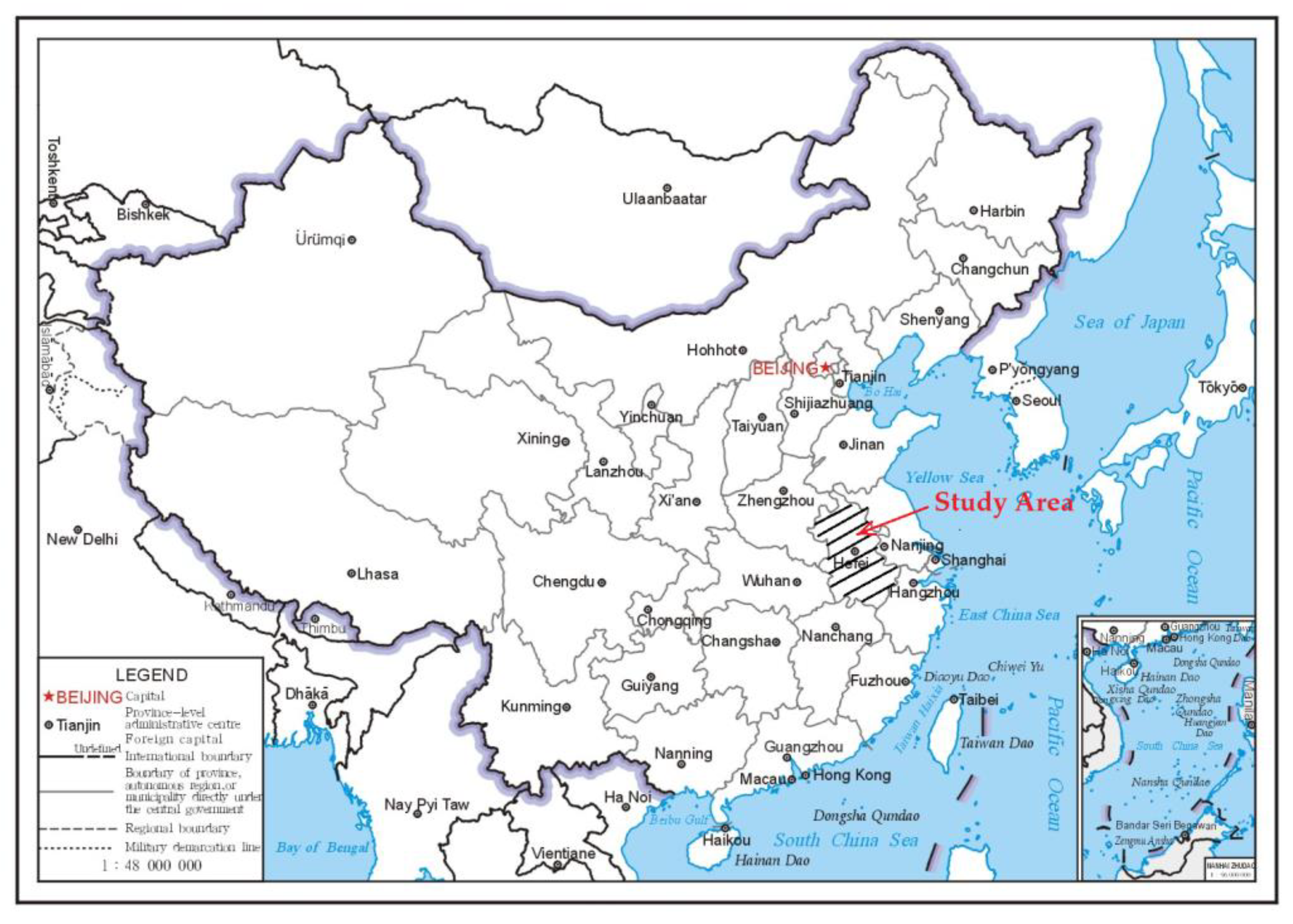
2.6.1. Overview of the Study Area

Anhui, the provincial capital of Hefei, is located in the Yangtze River Delta region. It is located between 114°54’ and 119°37’E longitude and 29°41’ and 34°38’N latitude and is in the middle and lower reaches of the Yangtze River. It is bordered by Jiangsu to the east, Henan and Hubei to the west, Zhejiang to the southeast, Jiangxi to the south, and Shandong to the north, with a width of 450 km from east to west and a length of 570 km from north to south. It covers an area of 140,100 km2 and a land area of 139,400 km2, accounting for 1.45% of the country and ranking 22nd. Anhui Province has a total of 16 prefecture-level cities under the jurisdiction of the province. The specific location of Anhui is as follows in Figure 2, in which the diagonally filled part is the location of Anhui Province.
Anhui Province is an important administrative region for the rapid economic development of eastern China, located in a typical north–south climate transition zone, crossing three major river basins: the Yangtze River Basin, the Huaihe River Basin, and the Xin’an River Basin. The north of the Huaihe River has a warm temperate semi-humid monsoon climate, and the south of the Huaihe River has a subhumid monsoon climate [30]. Its main characteristics are obvious monsoon, four distinct seasons, warm spring, more rainfall in summer, high temperature in autumn, and cold winter. Anhui is also located in the mid-latitudes; with the transition of the monsoon, precipitation has shown obvious seasonal changes, thus becoming one of the most significant regions of continental monsoon climate in China. Spring and autumn are the transition seasons between winter and summer and summer and summer and winter. The annual frost-free period is about 200–250 days. The average annual temperature is 14–17 °C, the average temperature in January is −4 °C, and the average temperature in July is 28–29 °C. The average annual precipitation is 773–1670 mm, showing the climate characteristics of more south and less north, many mountains, low flat hills, and abundant summer rainfall, accounting for 40–60% of the country’s perennial rainfall [31]. However, due to the influence of the changing average annual precipitation, the spatial distribution of water resources in Anhui Province is obviously uneven. The amount of water resources in the north is significantly lower than in the south, and the per capita water resources in cities vary significantly. Prominent water resource problems such as uneven distribution of water resources and poor water quality in Anhui Province have seriously restricted the sustainable economic and social development of Anhui Province.

2.6.2. Status of Sewage Discharge in the Base Year of Anhui Province

In order to implement the spirit of the Notice of the State Council on Printing and Distributing the Action Plan for Water Prevention and Control, adhere to the concept of green development, effectively strengthen the prevention and control of water pollution, strive to improve the quality of the water environment, and guarantee the health of people, combined with the actual situation of Anhui Province, the “13th Five-Year Plan for Environmental Protection of Anhui Province” [32] has been formulated. The plan clearly stipulates the emission reduction target for the total amount of water environment pollutants in 2020. By 2020, the total emission of chemical oxygen demand, ammonia nitrogen, sulfur dioxide, and nitrogen oxides in the province will be controlled within 785,000 tons, 83,000 tons, 403,000 tons, and 606,000 tons, respectively, down 9.9%, 14.3%, 16%, and 16% from 2015. In order to ensure the completion of the keyboard task of the total amount of water pollutants in Anhui Province during the 13th Five-Year Plan, it is urgent for us to conduct a systematic study on the allocation of regional pollution indicators for emission reduction. This study takes 2015 as the base year, takes total control in 2020 as the goal, allocates the proportion of pollutant reduction that should be borne by 16 municipalities in Anhui Province, and formulates a scientific and reasonable total water pollutant control plan. COD and NH3-N loads were selected as the main control factors to construct an optimal distribution model for water pollution load. In 2015, the total COD emissions in the province reached 870,900 tons, so at least 85,900 tons need to be reduced within five years; the total ammonia nitrogen emissions reached 96,800 tons, which needs to be reduced by 13,800 tons. According to the 2016 Anhui Statistical Yearbook [33] and the water resources annual reports provided by the municipal water bureaus, the specific values of water pollution discharge and evaluation indicators in each city can be calculated, as shown in Table 1. Among them, the total population of the province is 69.4911 million, the total GDP is CNY 2.254162 trillion, the total water resources are 91.412 billion m3, the total industrial output value is CNY 3.987566 trillion, and the total discharge of industrial wastewater is 714.3569 million tons.

3. Results and Discussions

3.1. Rationality Evaluation of the Current Situation of Pollutants

The rationality evaluation of the current situation of sewage discharge in Anhui Province is the premise for the implementation of the total allocation of water pollutants based on the principle of fairness. The rationality evaluation can use the contribution coefficient as an index to reflect the degree of unfairness in the distribution of pollution load outside the study area, while the environmental Gini coefficient shows the internal impact between control units, which can be used as the basis for distinguishing internal fairness [34].

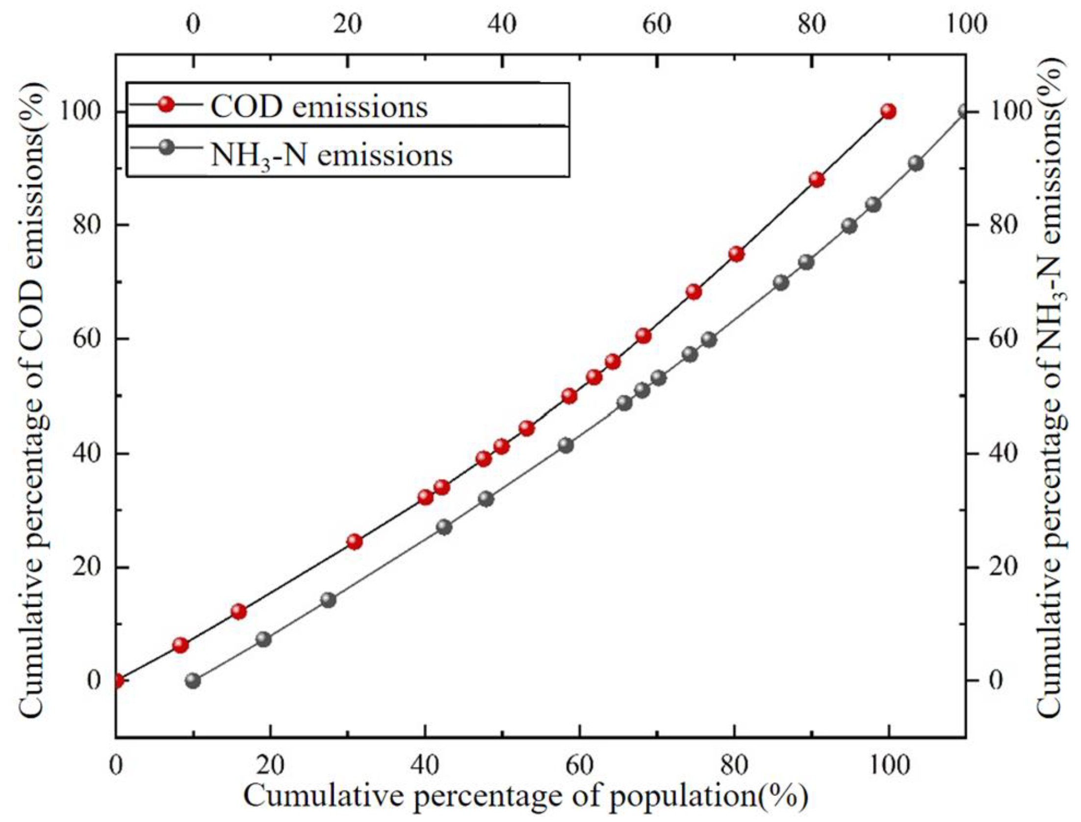
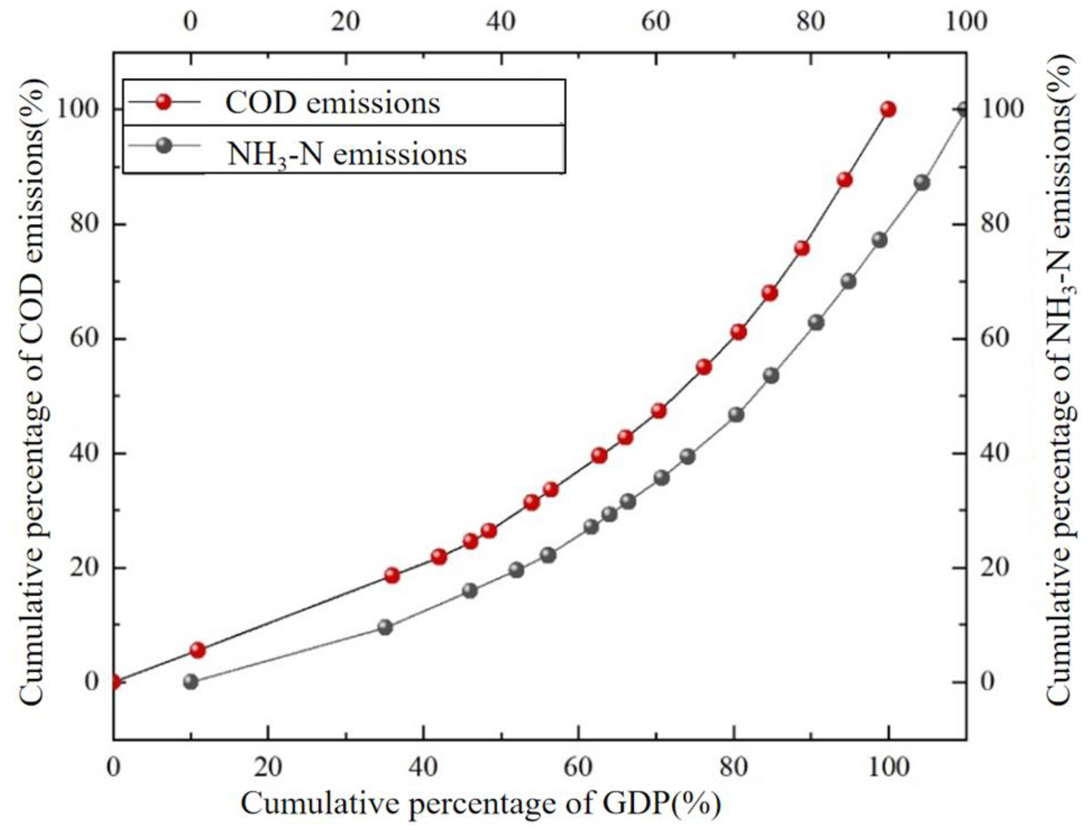
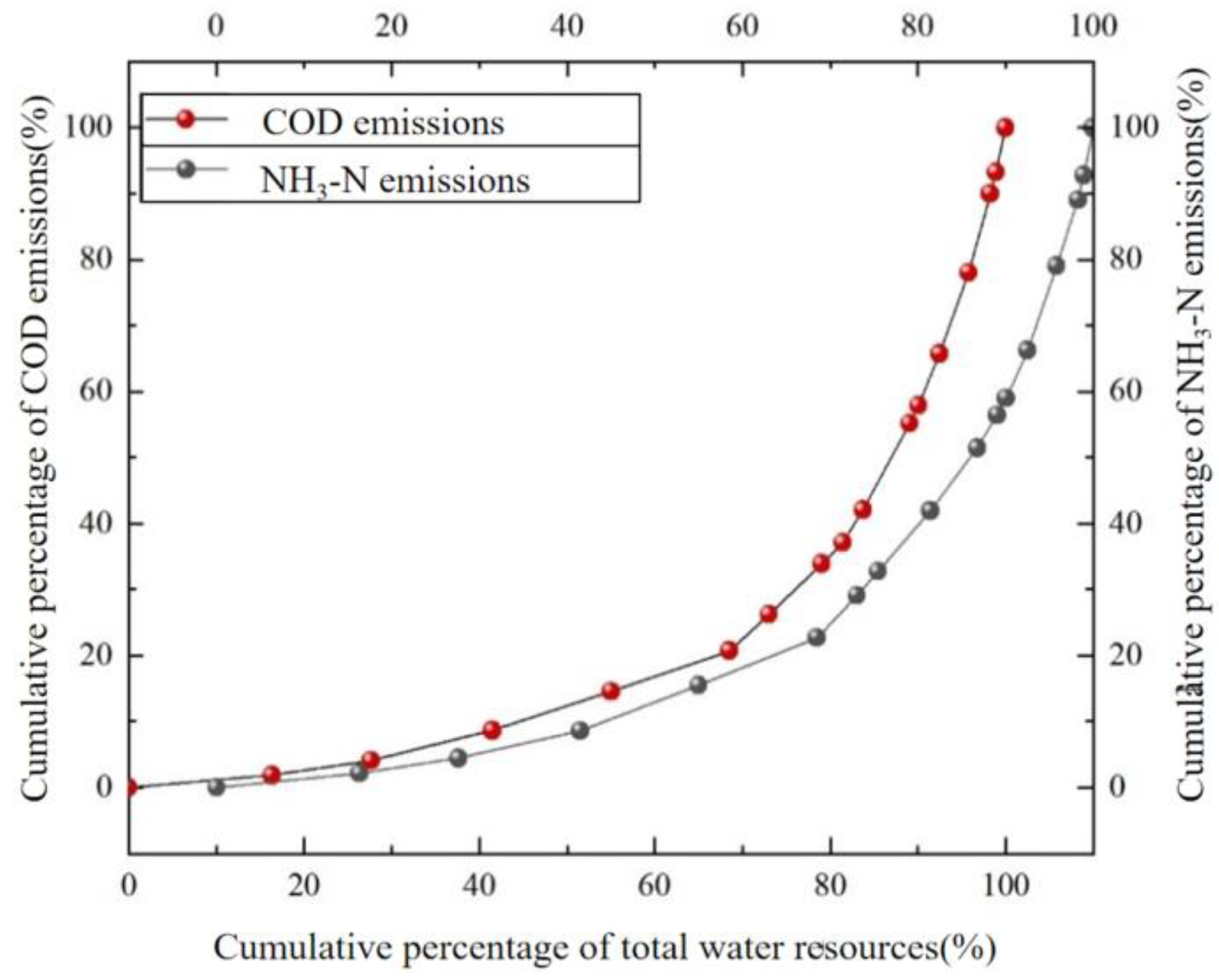
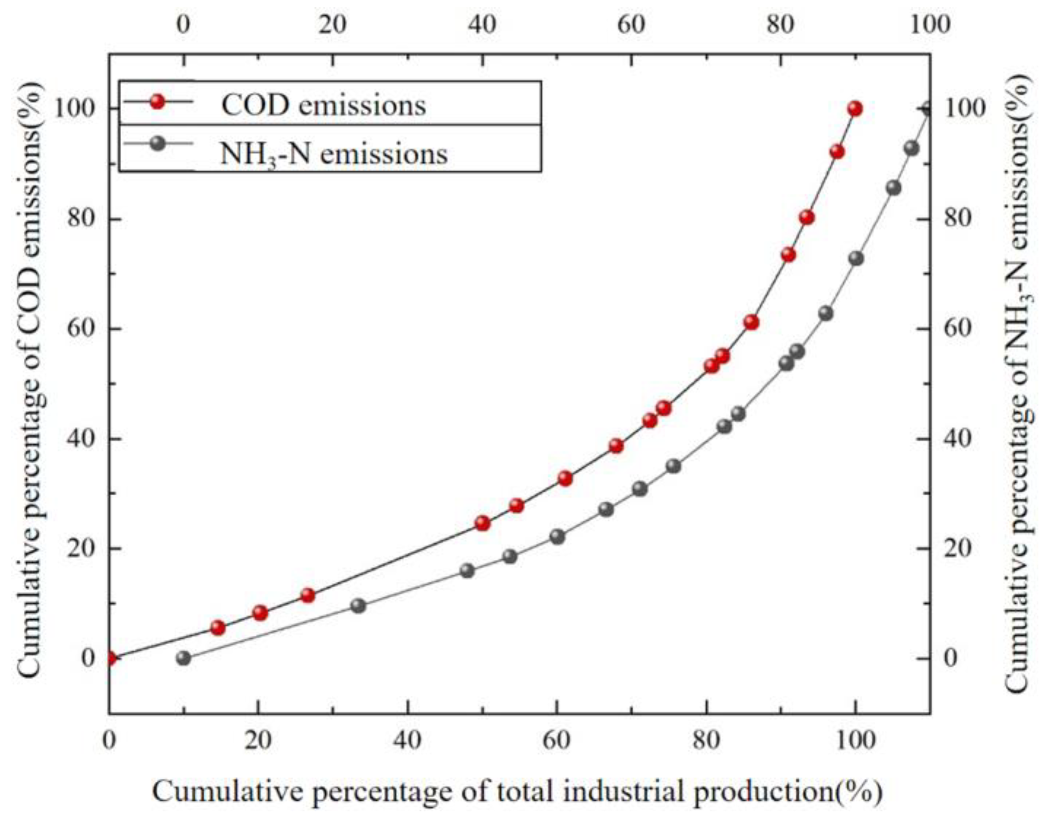
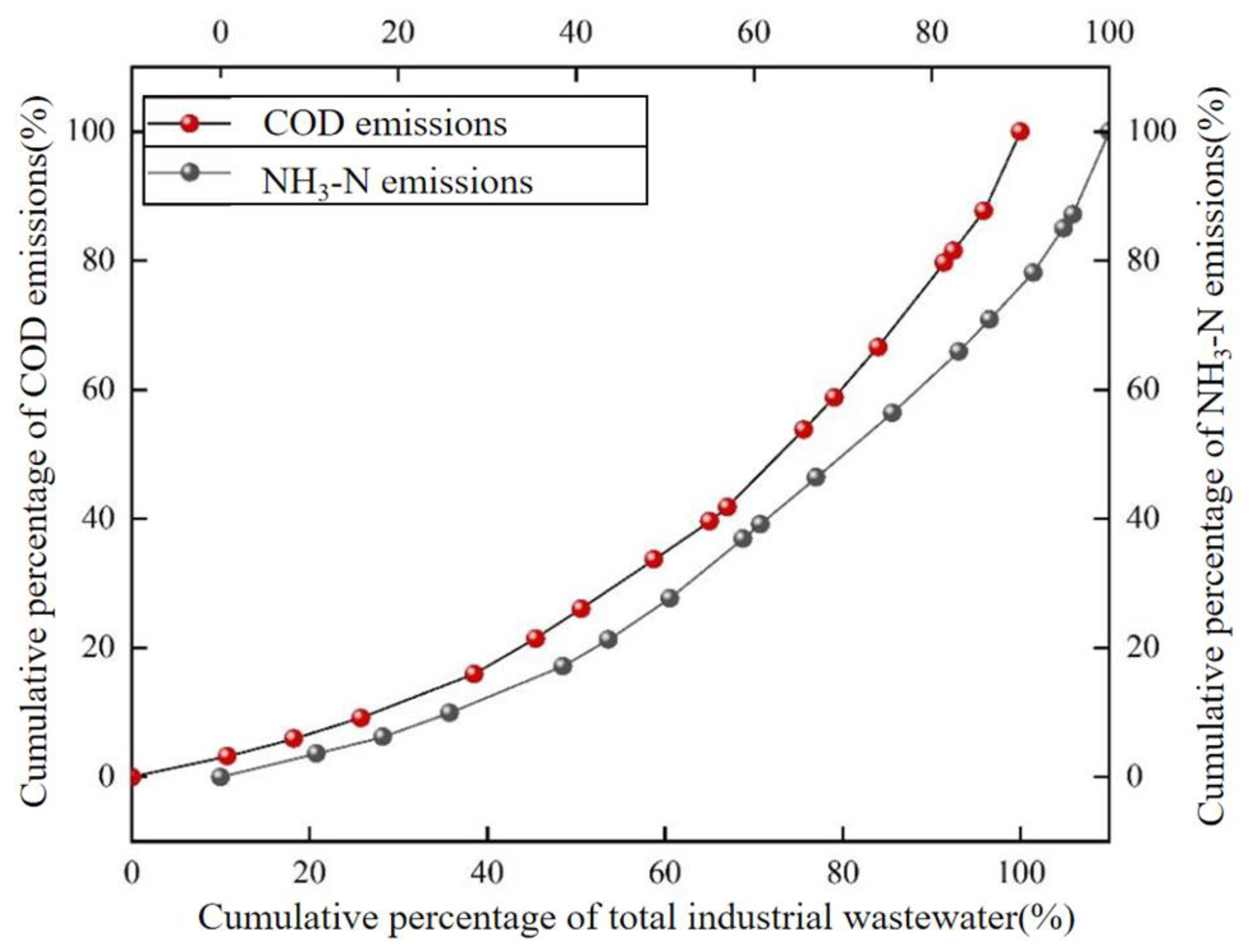
3.1.1. Study of the Regional Environmental Gini Coefficient

The Lorenz curve plots the cumulative proportion of GDP, population, water resources, industrial wastewater discharge, and industrial output value and the cumulative proportion of water pollutant (COD, ammonia nitrogen) emissions. When plotting the curve, the cumulative proportion should be sorted and calculated in order of the amount of sewage discharged from smallest to largest for each unit of index load. Take the plotting of the Lorenz curve of population-COD emissions as an example. Firstly, the municipalities of Anhui Province are sorted according to per capita COD emissions, and the cumulative proportion of population and COD emissions are statistically calculated according to the ranking, and the Lorenz curve chart (see Figure 3) is used to calculate the Gini coefficient of population-COD emissions according to the Lorenz curve. By analogy, according to the same method, the Lorenz curves of the remaining indicators and water pollutants can be plotted separately to obtain the Gini coefficient of all indicators, see Figure 3, Figure 4, Figure 5, Figure 6 and Figure 7.
In Figure 3, Figure 4, Figure 5, Figure 6 and Figure 7, the cities corresponding to the points on the Lorenz curve of different pollutant emissions under each indicator are different, and they are sorted according to the amount of pollutants per unit before making the map. By plotting the Lorenz curve and combining the trapezoidal area calculation method, the Gini coefficient G0(j) based on the corresponding pollutant emissions under different indicators is calculated, and the calculation results are shown in Table 2.
According to Figure 3, Figure 4, Figure 5, Figure 6 and Figure 7 and Table 2, it can be seen that the difference in the Gini coefficient of pollutants under different indicators is large, but the difference in the Gini coefficient of different pollutants in the same index is very small. This may be due to the similarity of the environmental media in which these two pollutants exist, so the distribution ratio in different regions is similar. The population-based COD and NH3-N Gini coefficients are less than 0.2 and are considered highly average. The COD and NH3-N Gini coefficients based on GDP, industrial output value, and industrial wastewater discharge are between ~0.2 and 0.4, which is already in a relatively unfair state, but does not exceed the warning value. COD and NH3-N Gini coefficients based on total water resources were the largest, exceeding the warning value of 0.4. It shows that there is still a big conflict between the distribution of pollutant loads in Anhui Province and the current situation of the regional water resources environment, and the pollutant discharge in different regions is not balanced enough, and it is necessary to optimize the distribution. In addition, the reduction of the Gini coefficient of the total water resources should be paid attention to in the total water pollution load allocation model.
The allocation of total water pollutants involves the adjustment of the Gini coefficient of multiple indicators, and the importance and impact of different indicators on the allocation are different. The allocation weights of each index involved in the fairness target in the allocation model are calculated by the entropy method, and the weights of population, GDP, total water resources, gross industrial production, and industrial wastewater discharge in the COD and NH3-N allocation models are calculated according to the data in Table 1, as shown in Table 3.

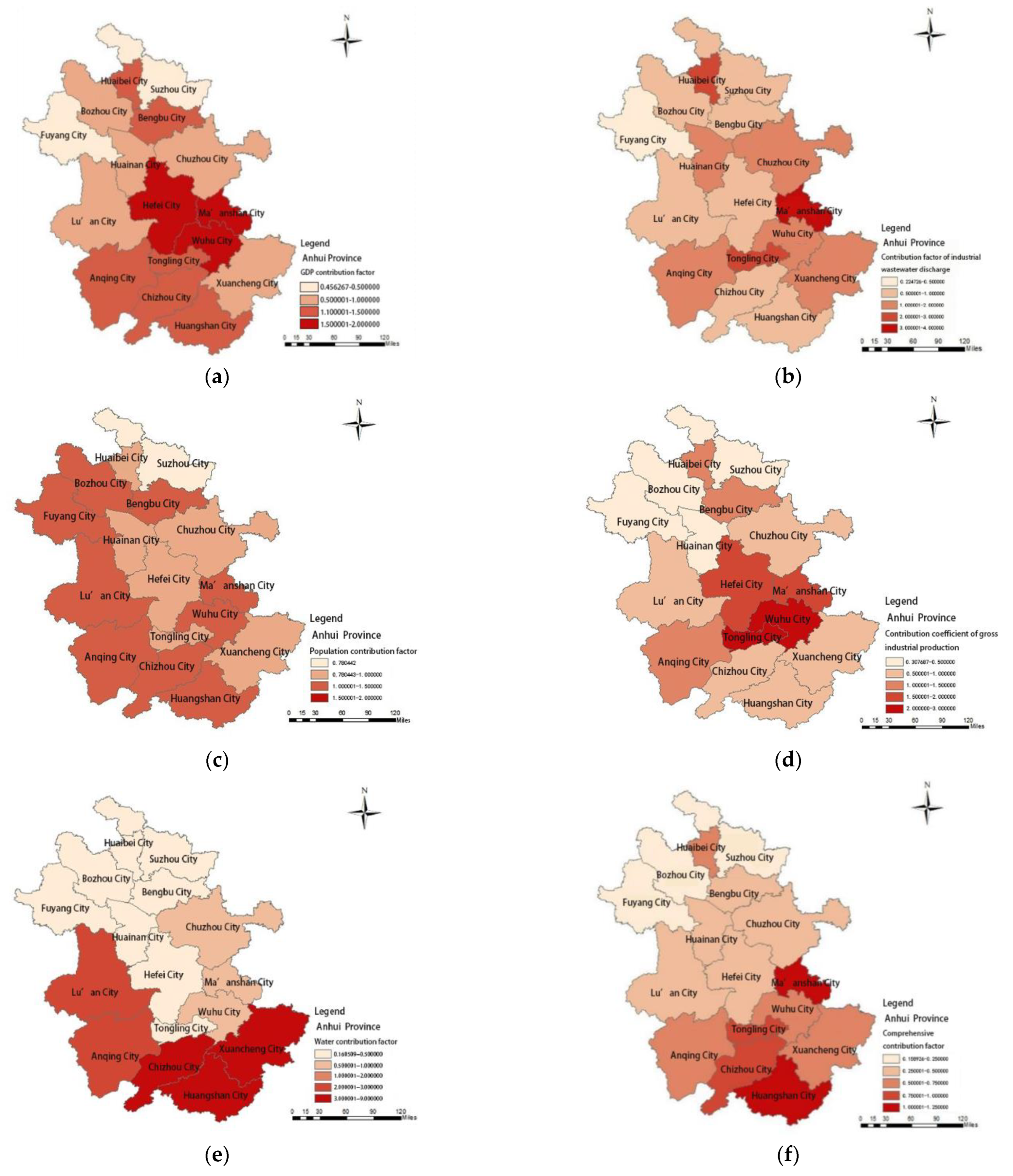
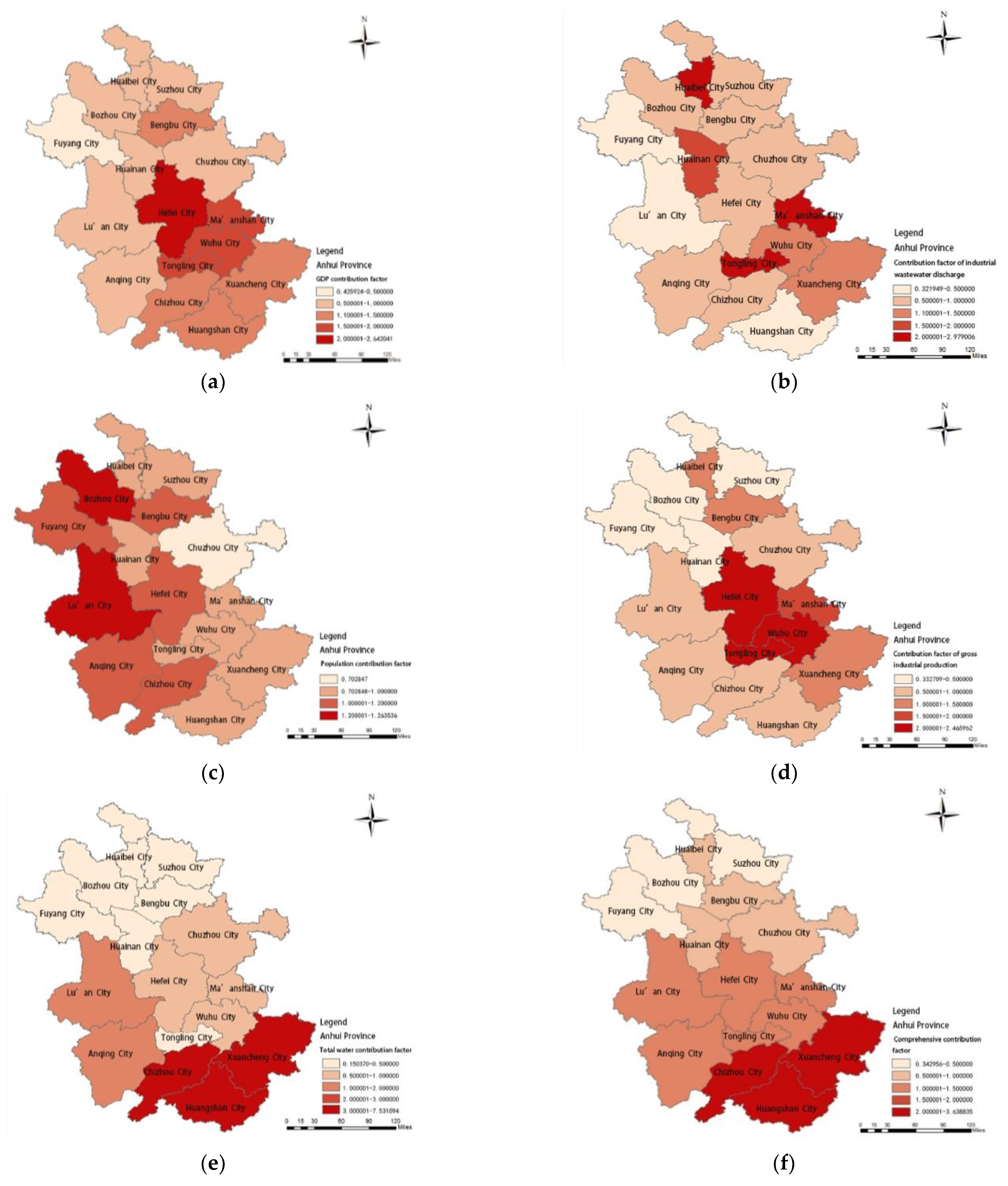
3.1.2. Study of the Environmental Contribution Factor of the Region

The rationality analysis of the current situation of sewage discharge in Anhui Province is the premise for the implementation of the total allocation of water pollutants based on the principle of fairness. The environmental Gini coefficient represents the internal influence between control units and can be used as a basis for distinguishing internal fairness [34]. The degree of fairness within the control unit should be quantified by reference to the contribution coefficient, and the main factors that cause the unfair gap should be identified, providing a basis for the fairness of subsequent distribution schemes. According to the above calculation formula of the specific values of each evaluation index and the environmental contribution coefficient in Anhui Province, the contribution coefficient under different indicators of the two pollutants was obtained, and the comprehensive contribution coefficient of each pollutant was calculated by combining the weight coefficient calculated by the entropy value method. The calculation results are statistically analyzed and plotted by ArcGIS Desktop 10.7.1 software (ESRI Inc., Redlands, CA, USA), and the specific distributions are shown in Figure 8 and Figure 9.
Figure 8 and Figure 9 show the distribution of contribution coefficients of COD and NH3-N indicators in Anhui Province in the benchmark year. Since the index (population) with a Gini coefficient of less than 0.2 is highly average, other indicators were selected for analysis. The Gini coefficient of total water resources-COD/NH3-N is the largest, and the analysis of the distribution map of the contribution coefficient to total water resources shows that the contribution coefficient of total water resources in Anhui Province shows an increasing trend from northwest to southeast. The contribution coefficients of the northern and central eastern parts of Anhui Province are less than 1. The water contribution coefficients of Fuyang, Bozhou, Huaibei, Suzhou, Bengbu, Huainan, and Tongling are less than 0.5, which is the main unfair factor. Combined with the data in Table 1, these cities accounted for 13.23% of the total water resources in Anhui Province, but COD and NH3-N emissions accounted for 49.81% and 48.56% of the total pollutant emissions. This shows a high degree of inequity in the indicator of total water resources. Due to the excessive weight of the index of total water resources, the distribution map of the comprehensive contribution coefficient of COD/NH3-N is basically consistent with the distribution map of the contribution coefficient of total water resources. Regional differences in total water resources are a major contributor to the uneven distribution of pollutants, indicating that the amount of water resources varies from region to region and the rate of economic development. Therefore, for regions with a large amount of water resources, the amount of pollutants allocated should be increased to indirectly promote the development of a regional economy. Areas with less water resources should pay attention to controlling and reducing the allocation of pollutants to control the discharge of pollutants from the source and avoid pollutants exceeding the carrying capacity of the water environment. The analysis of the contribution coefficient of GDP shows that the contribution coefficients of Hefei, Wuhu, Ma’anshan, and Tongling are greater than 1 based on the two pollutants, among which Hefei and Wuhu are among the best. It shows that the contribution rate of the city’s GDP is greater than the contribution rate of pollutant emissions, and the benefits brought by the discharge of pollutants are relatively high, which is manifested as a green economic development model. The contribution coefficients of Fuyang, Suzhou, Lu’an, Huainan, Bozhou, and Chuzhou are less than 1, especially Fuyang City, which is less than 0.5, which is the main factor causing inequality. Combined with the distribution map of the contribution coefficient of gross industrial production-COD/NH3-N, it can be found that the distribution of the two is basically the same in Anhui Province, indicating that the main source of GDP in Anhui Province is industrial production. In terms of future economic development, it is necessary to gradually realize industrial upgrading, reduce or even abandon high-pollution, low-value-added industries, and improve the efficiency of pollutant treatment.

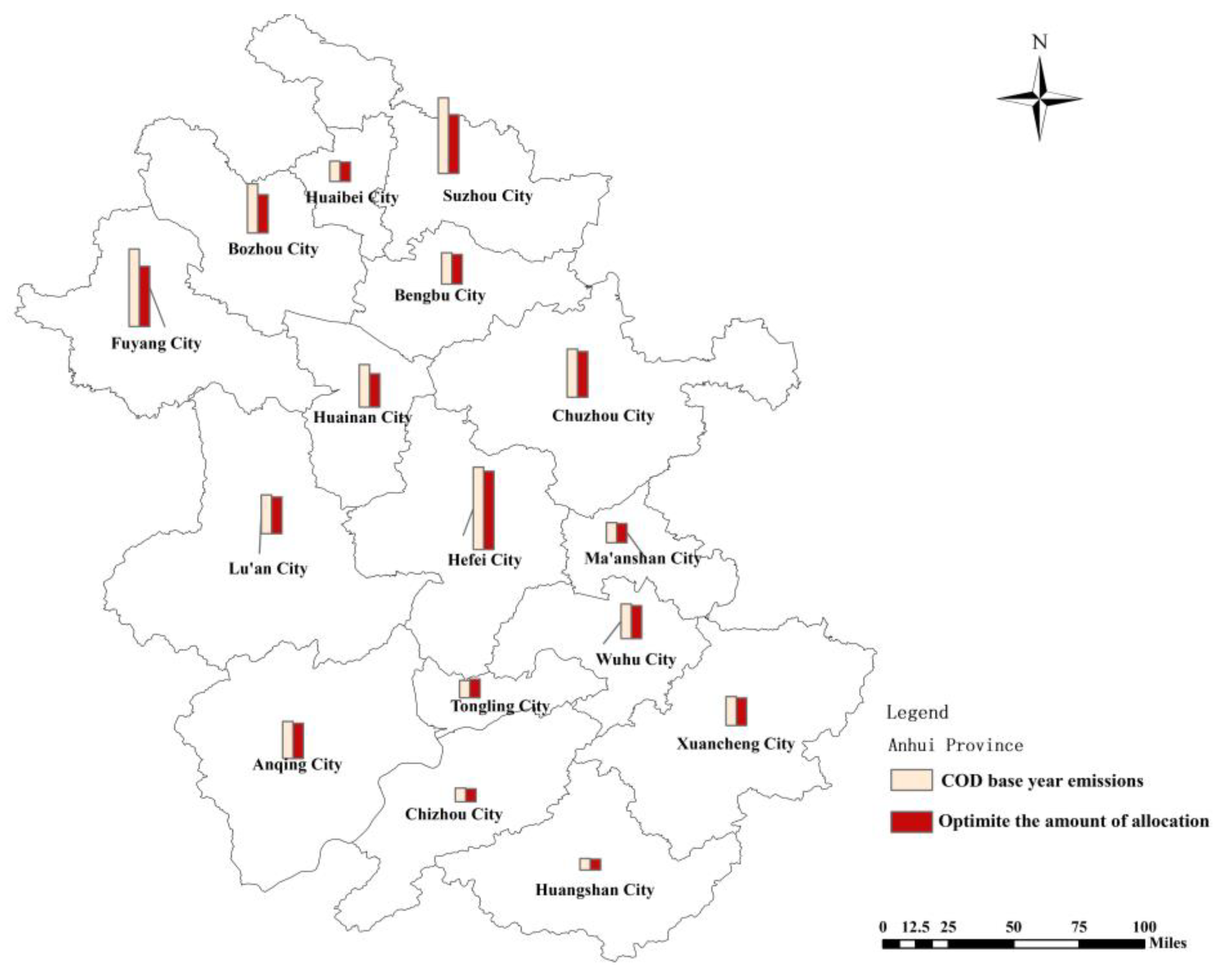
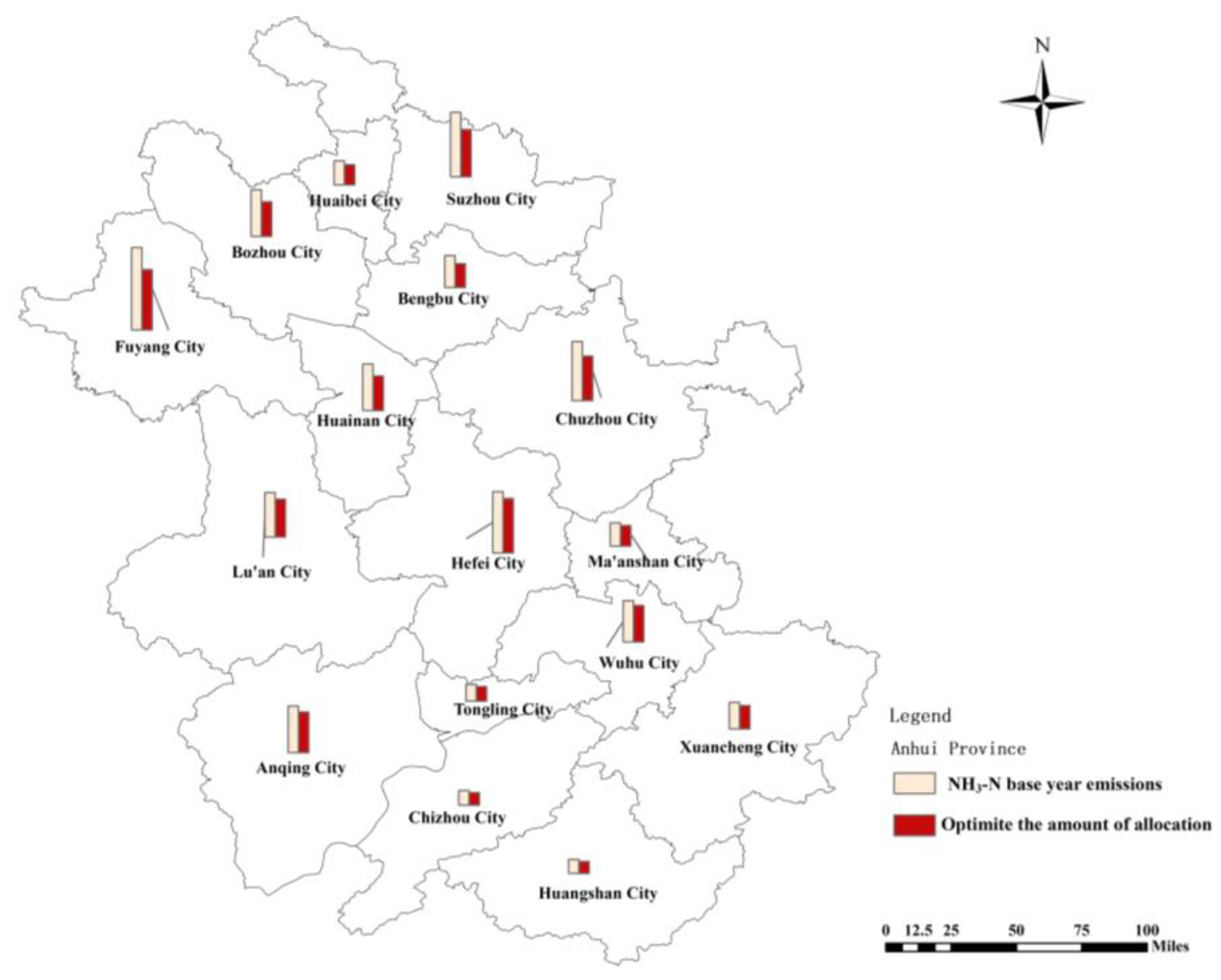
3.2. Optimal Allocation Results of Pollution Load in Anhui Province

Optimal allocation is solved by combining the model established by Equation (8)–(11) above and the solution method proposed in this paper. In the model of the Gini coefficient constraint, appropriate relaxation is given to the index constraint where the Gini coefficient is less than the warning value. The scaling amount is 10%, and the current Gini coefficient in the fairness constraint is ranged. For indicator constraints where the Gini coefficient is greater than the warning value, there is no need to give loose restrictions. Then, the Gini (COD-population) ≤ [0.11, 0.121], Gini(COD-GDP) ≤ [0.30, 0.33], Gini (COD-Industrial Production) ≤ [0.33, 0.363], and Gini (COD-industrial wastewater discharge) ≤ [0.34, 0.374], ammonia nitrogen allocation constraints are similar. In the allocation constraint of pollutant reduction rate, by 2020, the province’s chemical oxygen demand and ammonia nitrogen emissions will be reduced by 9.9% and 14.3%, respectively, compared with the base year. In order to ensure the realization of the reduction target and the optimal solution value of the model goal, the feasible domain should be appropriately increased within a reasonable range. It is advisable to set the chemical oxygen demand reduction rate of each sub-region at 5%~20% and the reduction rate of ammonia nitrogen at 10~30%. Among them, the lower limit of the reduction rate is the minimum reduction task that needs to be completed during the “13th Five-Year Plan” period in the study area, and no loose restrictions are given. In order to better reflect the inaccuracy and incompleteness of statistical data information, and also to improve the flexibility of decision-making schemes, the upper limit can be fuzzy, and the extension can be 5%. Therefore, the upper limit of COD emissions in each sub-region is Umax (COD) = [20%, 25%], and the upper limit of ammonia nitrogen emissions is Umax (NH3-N) = [30%, 35%].
During the model-solving process, the regularization factor α is determined to be 1 and β to 100,000 according to the size of the allocation target value. The solution process is based on Matlab software programming. The GA parameters are designed as follows through multiple algorithm debugging: Monte Carlo sampling times are 8000; genetic algorithm population size, popsize = 100; crossover probability, 0.8; mutation probability, 0.2; termination iteration genetic algebra, 500. Finally, the uncertain multi-objective optimization allocation results are obtained, as shown in Table 4.

3.3. Discussions

The optimization distribution results have been simulated 8000 times in Monte Carlo, and the optimization results have converged. Therefore, the final optimization result is based on the results of the 8000 times simulation. Each interval in the optimization allocation results is the result of 8000 times Monte Carlo simulations. In order to visualize the results, the values of each interval are averaged cumulatively and compared with the pollutant emissions in the base year. We plotted the distribution in ArcGIS software as follows (Figure 10 and Figure 11).
From the final pollutant discharge load distribution results of each sub-region, it can be seen that the water pollutant reduction quota of each municipality in Anhui Province is roughly similar to the proportion of pollutant discharge in the base year, which shows the fairness idea that the larger the pollutant discharge, the greater the regional reduction. However, it is not just that, it is also the result of a combination of contribution coefficients, Gini coefficients, and environmental, economic benefit coefficients. For example, in the distribution of the COD-comprehensive contribution coefficient, Fuyang City, Suzhou City, and Bozhou City have the lowest contribution coefficient. This means that the base year pollutant allocation is the highest in the three regions. Therefore, in the final allocation results, the allocation reduction of the three control areas was 24%, 22.9%, and 14.6%, respectively. Ranked in the top three in all control areas, the distribution results are reasonable and fair. On the contrary, for areas with a large contribution coefficient in the base year, such as Huangshan City, Xuancheng City, Chizhou City, and Ma’anshan City, which are more equitable in the basic comprehensive allocation, the reduction ratio in the final allocation result is relatively low. From the perspective of the environmental and economic benefit coefficient, Hefei’s base year GDP index is as high as CNY 566.027 billion, surpassing other research areas, indicating that its economic development momentum is better and more capable of supporting environmental protection expenditures generated by energy conservation and emission reduction. Therefore, in the final distribution results, the reduction ratio in Hefei is high.
In order to reflect the change in the Gini coefficient before and after optimization, Table 5 lists the comprehensive Gini coefficient of COD and NH3-N pollutants in the base year and the Gini coefficient after the optimized distribution scheme.
Combined with Table 5, it can be seen that the optimized comprehensive Gini coefficient decreased relative to the base year Gini coefficient, of which the comprehensive Gini coefficient after COD optimization decreased by 2.4~4.6%, and the comprehensive Gini coefficient after NH3-N optimization decreased by 25.1~32.5%. Obviously, COD is reduced relatively little. This is directly related to the pollutant reduction target in the 13th Five-Year Plan, and the appropriate emission reduction target needs to be formulated on the basis of a comprehensive review of the actual emission situation and the bearing capacity of the study area, and it is impossible to require a one-time emission reduction in order to reduce the Gini coefficient, which is often unrealistic. The control of total pollutant emissions is a long-term and continuous task, and the fairness of distribution is gradually optimized and adjusted [34].
After the above analysis and discussion, the optimal allocation results are in line with the principle that the pollutant reduction rate of the control unit with high water pollution discharge load should be increased accordingly under the premise of coordinated economic and social development. This verifies the feasibility and rationality of the model for optimal allocation of total water pollutant discharge in large areas.

4. Conclusions

(1)
Under the principles of sustainable development of the water environment, economic and social fairness, and efficiency, this paper proposes a comprehensive management model of multi-objective and uncertain optimization of the total amount of regional water pollution discharge and constructs a multi-objective decision-making optimization model of water pollution load (COD and NH3-N) allocation that takes into account economic optimum and fairness.
(2)
A solution method for the uncertain multi-objective allocation model is designed in this study, and the practicability and feasibility of the model solution method are verified by a case study. The results of multiple simulation–optimization can generate a series of decision schemes under uncertain objective functions and constraints and provide a more reasonable decision range for decision makers.
(3)
The model was applied to the allocation of total pollutant reduction in Anhui Province’s 13th Five-Year Plan for Environmental protection. Based on the environmental Gini coefficient, the rationality of the total pollutant distribution system in Anhui Province was evaluated, and the comprehensive Gini coefficients of COD and NH3-N were calculated to be 0.43152 and 0.42952, respectively. The Gini coefficients based on the total water resources were 0.59 and 0.57, which exceeded the warning value and were the main inequity factors.
(4)
After the optimization of water pollution load distribution, the comprehensive Gini coefficients of COD and NH3-N are reduced in different ranges. The comprehensive Gini coefficient decreases by 2.4~4.6% after COD optimization and 25.1~32.5% after NH3-N optimization. The control of total pollutant discharge is a long-term and continuous task, and the fairness of distribution is also gradually optimized and adjusted, which is the direction of further research.
The model proposed in this study takes into account the uncertain subjective and objective factors that have an important influence on the water pollutant emission targets and decision variables, so it can optimize the total emissions of the whole regional control unit in space and time and can be applied to the water pollution load allocation problem in similar provinces or regions.

Author Contributions

R.Z. and M.Z. constructed and conceived the project. W.C. and S.S. designed the research. R.Z., M.Z. and W.C. performed the research. R.Z., M.Z., W.C. and K.Z. analyzed the data. S.S. drew the figures. R.Z., W.C. and Y.S. wrote the paper. All authors have read and agreed to the published version of the manuscript.

Funding

This research was supported by Anhui Provincial Natural Science Foundation (2008085ME159, 2208085QE176), a Key project of the University Natural Science Research Project of Anhui Province (KJ2021A0505), Major university-level projects Anhui Polytechnic University (Xjky2020169), and the Science and Technology Project of Wuhu City (Grant No. 2022jc15).

Data Availability Statement

The data in this study are from the 2016 Anhui Provincial Statistical Yearbook and the annual water Resources report provided by municipal water bureaus.

Acknowledgments

We want to acknowledge the journal editors and anonymous reviewers for their valuable comments.

Conflicts of Interest

The authors declare no conflict of interest.

References

  1. Wang, Z.; Ye, A.; Liu, K.; Tan, L. Optimal Model of Desalination Planning Under Uncertainties in a Water Supply System. Water Resour. Manag. 2021, 35, 3277–3295. [Google Scholar] [CrossRef]
  2. Cui, Y.; Ning, S.; Jin, J.; Jiang, S.; Zhou, Y.; Wu, C. Quantitative Lasting Effects of Drought Stress at a Growth Stage on Soybean Evapotranspiration and Aboveground BIOMASS. Water 2021, 13, 18. [Google Scholar] [CrossRef]
  3. Pan, Z.; Jin, J.; Li, C.; Ning, S.; Zhou, R. A Connection Entropy Approach to Water Resources Vulnerability Analysis in a Changing Environment. Entropy 2017, 19, 591. [Google Scholar] [CrossRef] [Green Version]
  4. Zhang, M.; Wang, J.; Zhou, R. Attribution Analysis of Hydrological Drought Risk Under Climate Change and Human Activities: A Case Study on Kuye River Basin in China. Water 2019, 11, 1958. [Google Scholar] [CrossRef] [Green Version]
  5. Zhang, M.; Zhou, J.; Zhou, R. Interval Multi-Attribute Decision of Watershed Ecological Compensation Schemes Based on Projection Pursuit Cluster. Water 2018, 10, 1280. [Google Scholar] [CrossRef] [Green Version]
  6. Xiang, X.; Wu, X.; Chen, X.; Song, Q.; Xue, X. Integrating Topography and Soil Properties for Spatial Soil Moisture Storage Modeling. Water 2017, 9, 647. [Google Scholar] [CrossRef] [Green Version]
  7. Deng, Y.; Zheng, S.; Li, Z.; Hao, C.; Zheng, B. The innovation and future development of total pollutant control system. Res. Environ. Sci. 2021, 34, 382–388. [Google Scholar]
  8. Chen, L.; Han, L.; Tan, J.; Zhang, F.; Lin, Y. Optimization distribution model of point-point source pollution load in river network based on multi-section water quality standard. Water Resour. Prot. 2021, 37, 128–134+141. [Google Scholar]
  9. Yang, Y.; Zhao, Q.; Han, C.; Xing, C.; Song, L.; Hu, Z. Research on total amount allocation of sea and watershed water pollutants based on fairness principle. Mar. Environ. Sci. 2019, 38, 796–803. [Google Scholar]
  10. Zhang, X.; Wang, P.; He, Y.; Du, Z.; Luo, J.; Xie, J. Study of two-layer multi-objective optimization model for water pollution load distribution in rivers. J. Xi’an Univ. Technol. 2020, 36, 475–485. [Google Scholar]
  11. Li, R.; Shu, K. Model for wastewater load allocation based on multi-objective decision making. Acta Sci. Circumst. 2011, 31, 2814–2821. [Google Scholar]
  12. Wang, X.; Pang, M.; Zhao, M. Pollution Load Capacity Calculation Study Based on Multi-objective System in Trans-boundary Area, Plain River Network. Bull. Environ. Contam. Tox. 2021, 106, 600–607. [Google Scholar] [CrossRef] [PubMed]
  13. Liu, Q.; Li, Z.; Yao, G. Research on equity of total water pollutant distribution based on Gini coefficient. China Water Wastewater 2016, 32, 90–94. [Google Scholar]
  14. Wu, F.; Cao, Q.; Zhang, D.; Sun, F.; Shen, J. Allocation of flood drainage rights of Sunan Canal based on environmental Gini coefficient. J. Hohai Univ. (Nat. Sci.) 2020, 48, 314–319. [Google Scholar]
  15. Kolluru, M.; Semenenko, T. Income Inequalities in EU Countries: Gini Indicator Analysis. ECONOMICS-Innov. Econ. Res. 2021, 9, 125–142. [Google Scholar] [CrossRef]
  16. Zaeimi, M.B.; Rassafi, A.A. Designing an integrated municipal solid waste management system using a fuzzy chance-constrained programming model considering economic and environmental aspects under uncertainty. Waste Manag. 2021, 125, 268–279. [Google Scholar] [CrossRef]
  17. Liu, Q.; Jiang, J.; Jing, C.; Liu, Z.; Qi, J. A New Water Environmental Load and Allocation Modeling Framework at the Medium—Large Basin Scale. Water 2019, 11, 2398. [Google Scholar] [CrossRef]
  18. Wang, M.; Gong, H. Imbalanced Development and Economic Burden for Urban and Rural Wastewater Treatment in China—Discharge Limit Legislation. Sustainability 2018, 10, 2597. [Google Scholar] [CrossRef] [Green Version]
  19. Chen, W.; Zhang, M.; Zhao, W. Study on multi-objective optimal allocation of water resources system under uncertainties. J. Hydro. Eng. 2021, 40, 12–24. [Google Scholar]
  20. Xie, Y.; Zhou, X. Income inequality in today’s China. Proc. Natl. Acad. Sci. USA 2014, 111, 6928–6933. [Google Scholar] [CrossRef] [Green Version]
  21. Zhang, F. Study on the Total Pollution Distribution in the Middle Reaches of Fenhe Based on Information Entropy and Gini Coefficient Method. Master’s Thesis, Xi’an University of Technology, Xi’an, China, 2021. [Google Scholar]
  22. Shu, H.; Xiong, P. Construction of Gini Coefficient of a mixed environment and its Application in the evaluation of industrial economy and ecological spatial equilibrium. Math. Pract. Theory 2018, 48, 9–17. [Google Scholar]
  23. Steinberger, J.K.; Krausmann, F.; Eisenmenger, N. Global patterns of materials use: A socioeconomic and geophysical analysis. Ecol. Econ. 2010, 69, 1148–1158. [Google Scholar] [CrossRef]
  24. Cheng, Y.; Li, Y.; Zhu, X.; Shi, Y.; Zhu, Y.; Pan, H.; Xu, Y.; Cheng, Y. Total pollutant load allocation in plain river network based on the entropy-environmental Gini coefficient method. J. Lake Sci. 2020, 32, 619–628. [Google Scholar]
  25. Shu, K. Model and Method of Water Waste Loads Allocation in a Region-Case of Chaohu Lake Basin. Master’s Thesis, Hefei University of Technology, Hefei, China, 2010. [Google Scholar]
  26. Yu, S.; Lu, H. Integrated watershed management through multi-level and stepwise optimization for allocation of total load of water pollutants at large scales. Environ. Earth Sci. 2018, 77, 373. [Google Scholar] [CrossRef]
  27. Wu, W.; Jiang, H.; Duan, Y.; Liu, N.; Lu, Y.; Zhang, W.; Yu, S. Application of total water pollutant load distribution in control-unit based on the environmental Gini coefficient. China Popul. Resour. Environ. 2017, 27, 8–16. [Google Scholar]
  28. Marler, R.T.; Arora, J.S. The weighted sum method for multi-objective optimization: New insights. Struct. Multidiscip. Optim. 2010, 41, 853–862. [Google Scholar] [CrossRef]
  29. Jin, J.; Ding, J. Genetic Algorithm and Its Application in Water Science; Sichuan University Press: Chengdu, China, 2000. [Google Scholar]
  30. Li, C.; Chen, J.; Wang, R.; Huang, J.; Qian, Z.; Xu, Y. Multi-indices analysis of heavy precipitation changes in Anhui Province, China. Meteorol. Atmos. Phys. 2021, 133, 1317–1325. [Google Scholar] [CrossRef]
  31. Tan, W.; Zhang, C.; Liu, X. Research on the compilation of the Atlas of the First National Census of Geographical Conditions in Anhui Province. Intell. City 2020, 6, 52–53. [Google Scholar]
  32. Anhui Provincial Department of Environmental Protection. 13th Five-Year Plan for Environmental Protection of Anhui Province; Anhui Provincial People’s Government: Hefei, China, 2017.
  33. Anhui Provincial Bureau of Statistics. Anhui Statistical Yearbook-2016; China Statistics Press: Beijing, China, 2016. [Google Scholar]
  34. Qin, D.; Wei, A.; Lu, S.; Luo, Y.; Liao, Y.; Yi, M.; Song, B. Total water pollutant load allocation in Dongting Lake area based on the environmental Gini coefficient method. Res. Environ. Sci. 2013, 26, 8–15. [Google Scholar]
Figure 1. Schematic diagram of Lorentz curve. A is the area between the actual distribution curve and the absolute equal distribution curve; B is the area under the actual distribution curve.
Water 15 00309 g001
Figure 2. Location of Anhui Province in China. From the website of the Ministry of Natural Resources of the People’s Republic of China, Figure Number: GS (2019) No.1674, downloaded at: http://bzdt.ch.mnr.gov.cn/index.html (accessed on 10 November 2022). The broken line indicated by the arrow on the map is the study area of Anhui Province.
Water 15 00309 g002
Figure 3. Lorenz curves of COD and NH3-N based on population.
Water 15 00309 g003
Figure 4. Lorenz curves of COD and NH3-N based on GDP indicators.
Water 15 00309 g004
Figure 5. Lorenz curves of COD and NH3-N based on total water resources indicators.
Water 15 00309 g005
Figure 6. Lorenz curves of COD and NH3-N based on total industrial output indicators.
Water 15 00309 g006
Figure 7. Lorenz curves of COD and NH3-N based on discharge of industrial wastewater indicators.
Water 15 00309 g007
Figure 8. Distribution of COD index contribution coefficient in the benchmark year of Anhui Province. (a) GDP contribution factor. (b) Contribution factor of industrial wastewater discharge. (c) Population contribution factor. (d) Contribution factor of gross industrial production. (e) Total water contribution factor. (f) Comprehensive contribution factor.
Water 15 00309 g008
Figure 9. Distribution of NH3-N index contribution coefficient in Anhui Province in the benchmark year. (a) GDP contribution factor. (b) Contribution factor of industrial wastewater discharge. (c) Population contribution factor. (d) Contribution factor of gross industrial production. (e) Total water contribution factor. (f) Comprehensive contribution factor.
Water 15 00309 g009
Figure 10. Distribution chart of comparison between COD optimized distribution results and base year.
Water 15 00309 g010
Figure 11. Comparison distribution of NH3-N optimized distribution results with base year.
Water 15 00309 g011
Table 1. Specific values of water pollution emissions and evaluation indicators of cities in Anhui Province in 2015.
RegionPollutant DischargeIndicators of Evaluation
COD (10,000 tons)NH3-N (10,000 tons)Population
(10,000 People)
GDP
(CNY 100 million)
Water
Volume
(100 million m3)
Industrial
Output Value
(CNY 100 million)
Wastewater
Discharge
(10,000 tons)
Hefei11.40.92717.725660.2748.639345.595334.98
HuaiBei2.80.36216.5760.395.991814.65377.67
Bozhou6.810.7634.95942.6122.25959.393501.66
Suzhou10.430.97649.511235.8322.391,623.256126.77
Bengbu4.330.48376.351253.0520.822,596.822474.02
Fuyang10.731.241042.651267.4530.281989.692946.11
Huainan5.90.7383.39901.089.94970.429112.06
Chuzhou6.670.89449.061305.754.832567.115859.72
Lu’an5.360.67580.531016.49123.571542.12443.29
Ma’anshan2.790.35228.51365.322.152540.757694.53
Wuhu4.80.62384.792457.3241.345829.014933.27
Xuancheng4.020.4279.95971.46126.681796.383664.98
Tongling2.380.25170.43911.69.252269.015338.25
Chizhou1.920.22161.61544.74103.13740.431422.11
Anqing5.150.7525.481417.43123.522723.164469.63
Huangshan 1.60.21147.69530.9149.35567.95736.62
Total87.099.686949.1122,541.6914.1239,875.771,435.7
Table 2. Gini coefficient of corresponding pollutants under each evaluation index in Anhui Province in 2015.
Evaluation IndicatorsPopulationGDPTotal Water ResourcesGross Industrial OutputIndustrial Wastewater
Discharge
COD0.110.300.590.330.34
NH3-N0.100.320.570.390.32
Table 3. Information entropy weight of each evaluation index in fairness objective.
PollutantsPopulationGDPTotal Water
Resources
Gross Industrial OutputIndustrial Wastewater
Discharge
COD0.0220.1300.4170.2470.184
NH3-N0.0210.1260.4300.2320.191
Table 4. Water pollution load distribution and reduction plan of Anhui Province in 2020.
PollutantsRegionBenchmark Annual Emissions (×104t)Distributed
Emissions (×104t)
Amount of
Reduction (×104t)
Rate of
Reduction/%
Reduction of Quotas/%
CODHefei11.4[10.69, 10.83][0.57, 0.71][5.0, 6.2]6.5
HuaiBei2.8[2.51, 2.66][0.14, 0.29][5.0, 10.4]2.1
Bozhou6.81[5.11, 5.60][1.21, 1.70][17.8, 24.9]14.6
Suzhou10.43[7.82, 8.52][1.91, 2.61][18.3, 25.0]22.9
Bengbu4.33[3.97, 4.11][0.22, 0.36][5.1, 8.3]2.9
Fuyang10.73[8.05, 8.68][2.05, 2.68][19.1, 25.0]24
Huainan5.09[4.43, 4.83][0.26, 0.66][5.1, 13.0]4.4
Chuzhou6.67[6.11, 6.34][0.33, 0.56][5.0, 8.4]4.4
Lu’an5.36[4.76, 5.09][0.27, 0.60][5.0, 11.2]4.2
Ma’anshan2.79[2.56, 2.65][0.14, 0.23][5.0, 8.2]1.8
Wuhu4.80[4.47, 4.56][0.24, 0.33][5.0, 6.9]2.9
Xuancheng4.02[3.75, 3.82][0.20, 0.27][5.0, 6.7]2.4
Tongling2.38[2.16, 2.26][0.12, 0.22][5.0, 9.0]1.6
Chizhou1.92[1.72, 1.82][0.10, 0.20][5.0, 10.4]1.5
Anqing5.15[4.76, 4.89][0.26, 0.39][5.0, 7.6]3.2
Huangshan1.60[1.46, 1.52][0.08, 0.14][5.0, 8.8]1.0
Total87.09[74.33, 78.28][8.00, 11.95][9.2, 13.7]100
NH3-NHefei0.92[0.68, 0.828][0.09, 0.24][10, 26.1]8.4
HuaiBei0.36[0.25, 0.32][0.04, 0.11][11, 30.6]3.8
Bozhou0.7[0.49, 0.63][0.07, 0.21][10, 30]7.1
Suzhou0.97[0.68, 0.84][0.13, 0.29][13.4, 29.9]10.6
Bengbu0.48[0.34, 0.43][0.05, 0.14][10.4, 29.2]4.8
Fuyang1.24[0.87, 1.03][0.21, 0.37][16.9, 29.8]14.7
Huainan0.7[0.49, 0.63][0.07, 0.21][10, 30.0]7.1
Chuzhou0.89[0.62, 0.80][0.09, 0.27][10.1, 30.3]9.1
Lu’an0.67[0.48, 0.60][0.07, 0.19][10.4, 28.4]6.6
Ma’anshan0.35[0.25, 0.31][0.04, 0.10][11.4, 28.6]3.5
Wuhu0.62[0.44, 0.55][0.07, 0.18][11.3, 29.0]6.3
Xuancheng0.4[0.29, 0.36][0.04, 0.11][10, 27.5]3.8
Tongling0.25[0.18, 0.22][0.03, 0.07][12.0, 28]2.5
Chizhou0.22[0.16, 0.19][0.03, 0.06][13.6, 27.3]2.3
Anqing0.7[0.49, 0.63][0.07, 0.21][10.0, 30]7.1
Huangshan0.21[0.15, 0.18][0.03, 0.06][14.2, 28.6]2.3
Total9.68[6.86, 8.60][1.13, 2.82][11.7, 29.1]100
Table 5. Changes in the comprehensive Gini coefficient after optimal allocation.
PollutantsBenchmark YearAfter OptimizationRange of Reduction
COD0.4315[0.4117, 0.4210][−4.6%, −2.4%]
NH3-N0.4295[0.2901, 0.3216][−32.5%, −25.1%]
Disclaimer/Publisher’s Note: The statements, opinions and data contained in all publications are solely those of the individual author(s) and contributor(s) and not of MDPI and/or the editor(s). MDPI and/or the editor(s) disclaim responsibility for any injury to people or property resulting from any ideas, methods, instructions or products referred to in the content.

