
Bridge Pier Scour in Complex Environments: The Case of Chacao Channel in Chile


Abstract
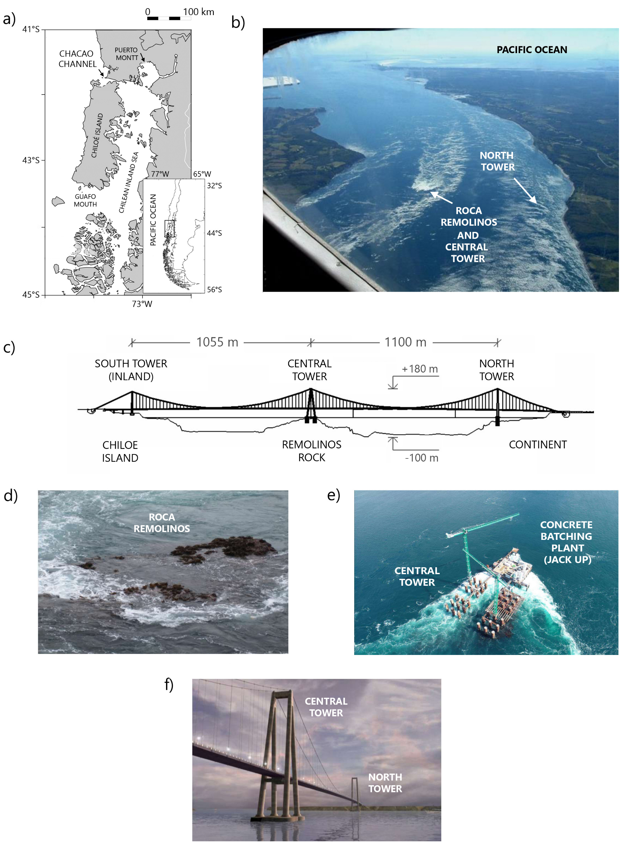
1. Introduction
2. Methodology
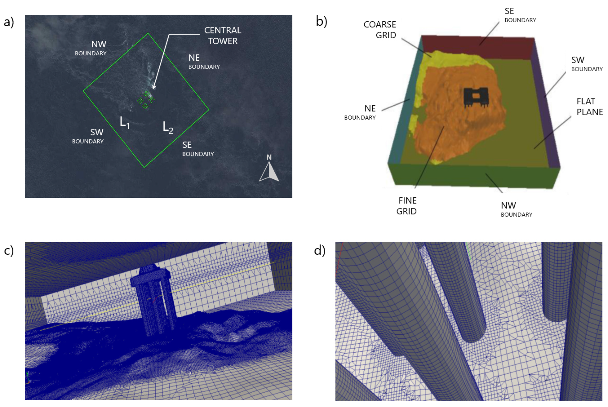
2.1. Modelling Flow Fields
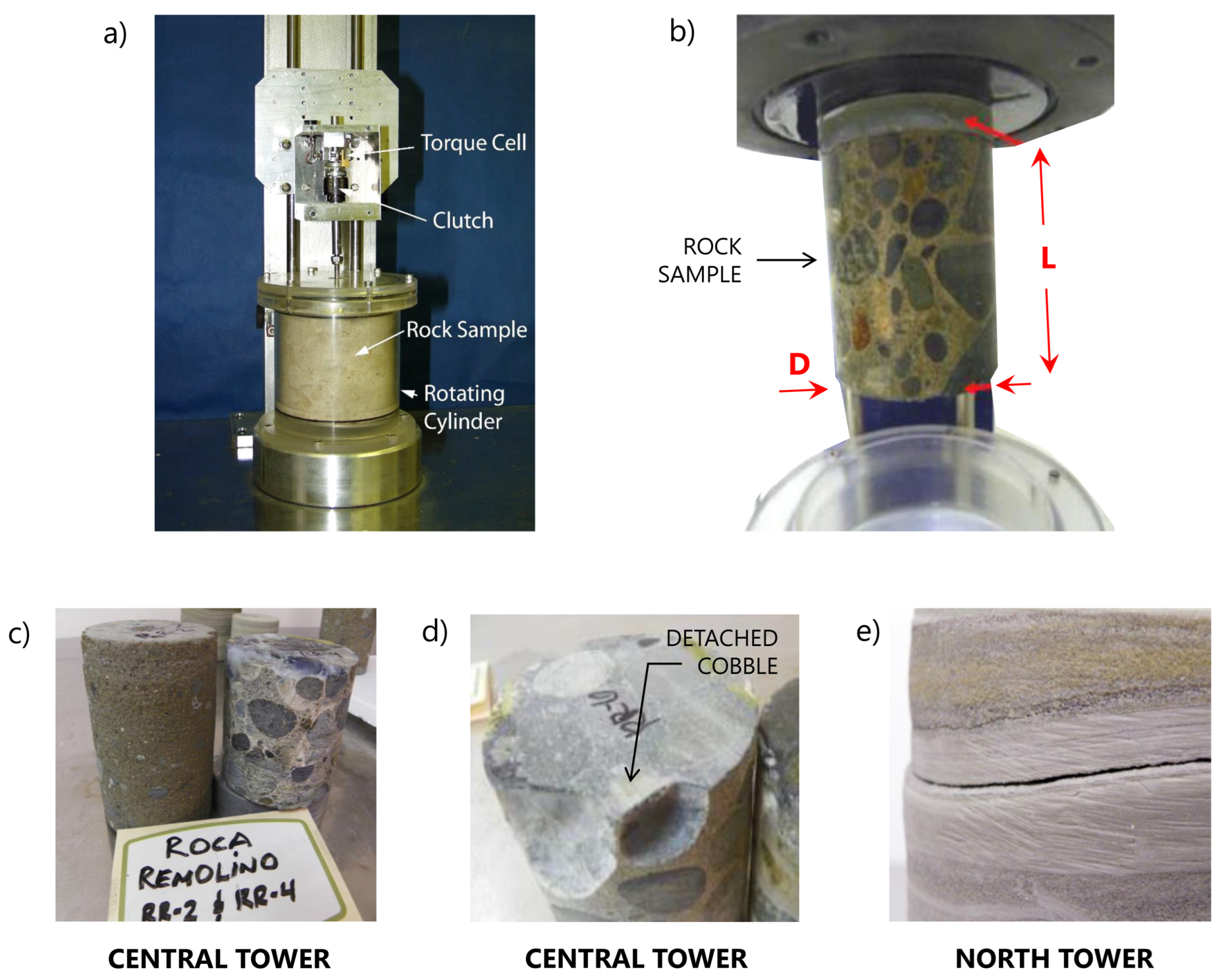
2.2. Estimation of the Erosion Rate in Earth Materials
2.3. Erosion and Scour in Central Tower
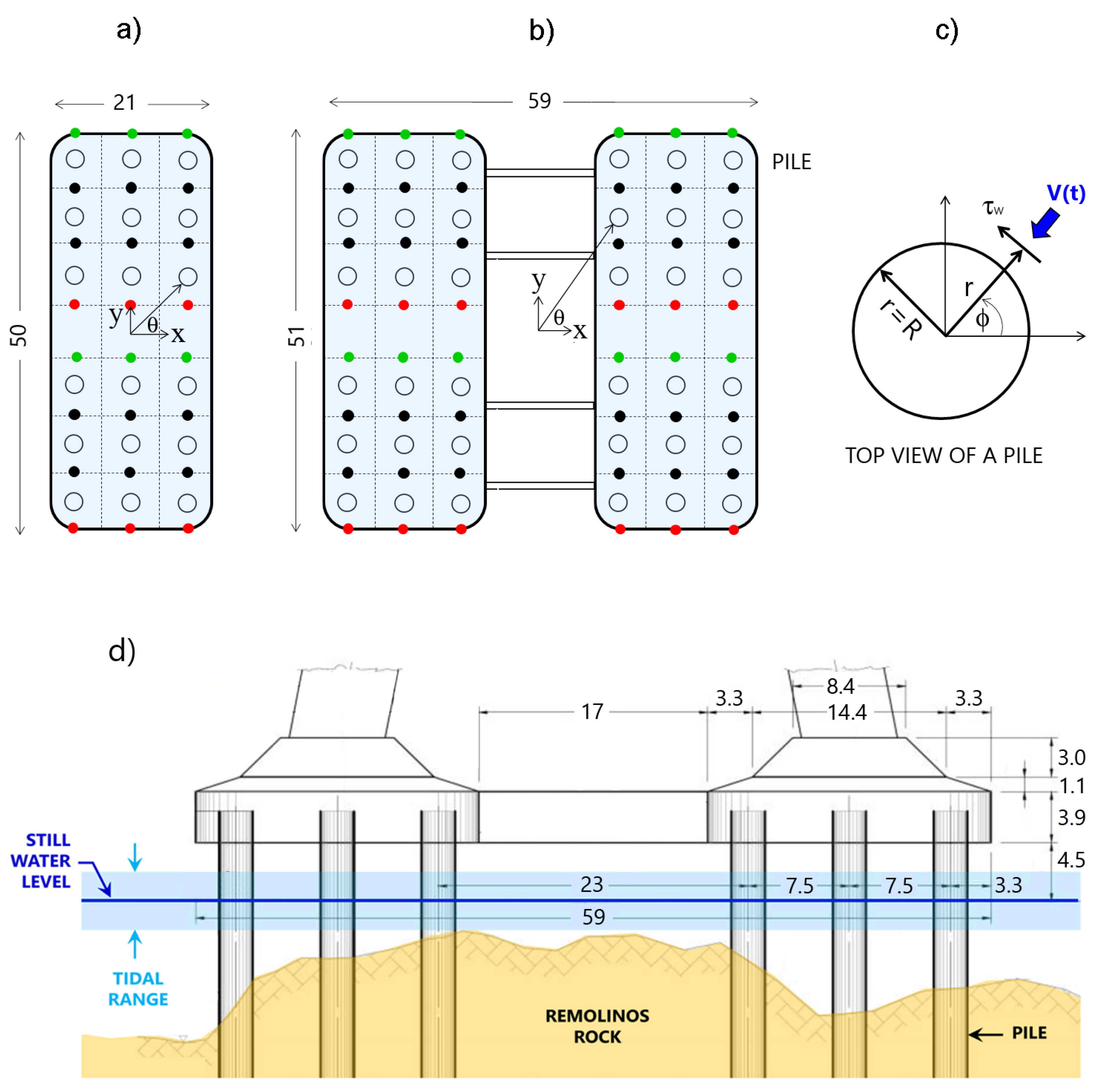
2.4. Erosion and Scour at North Tower Site
3. Results for North Tower
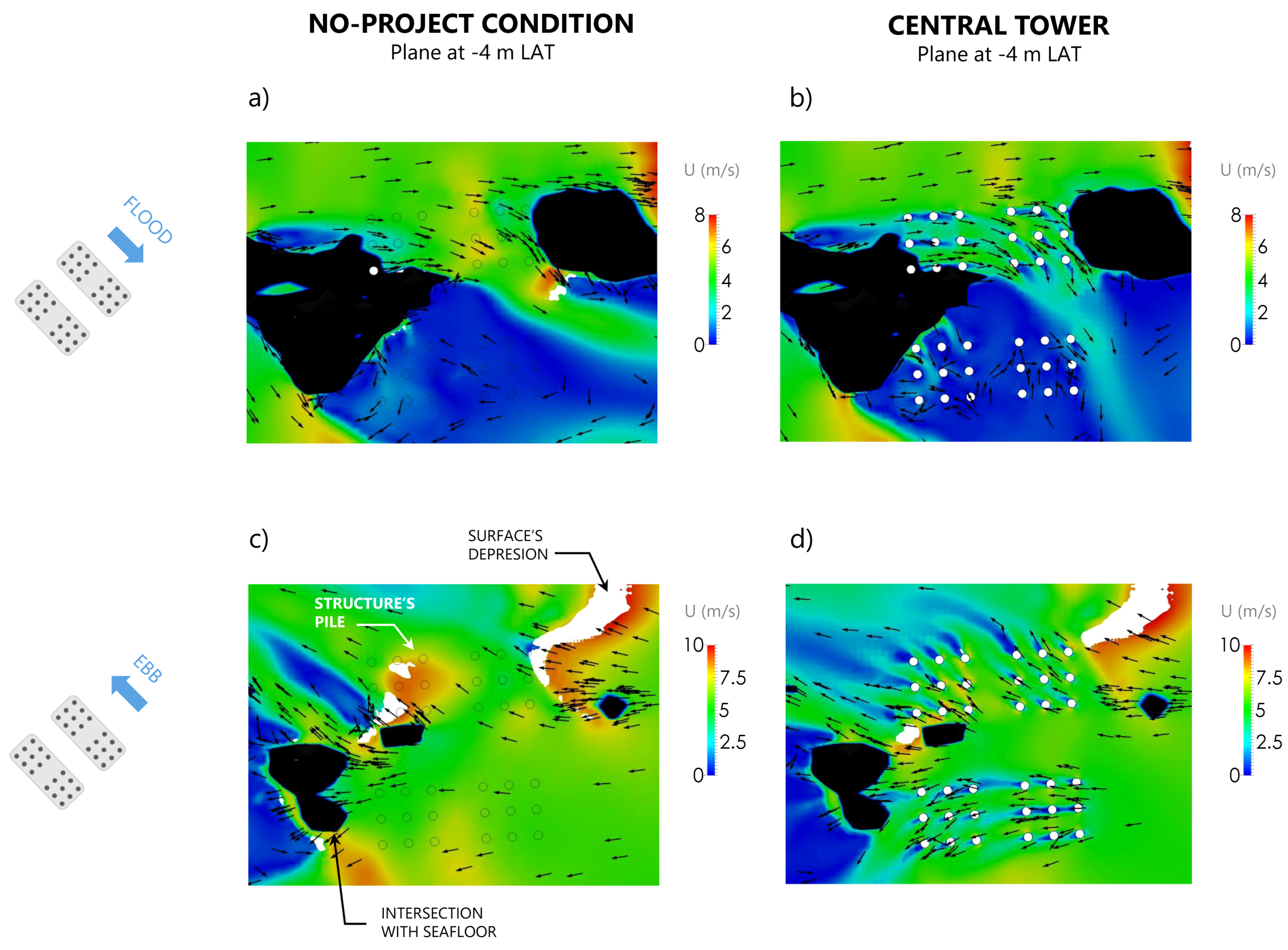
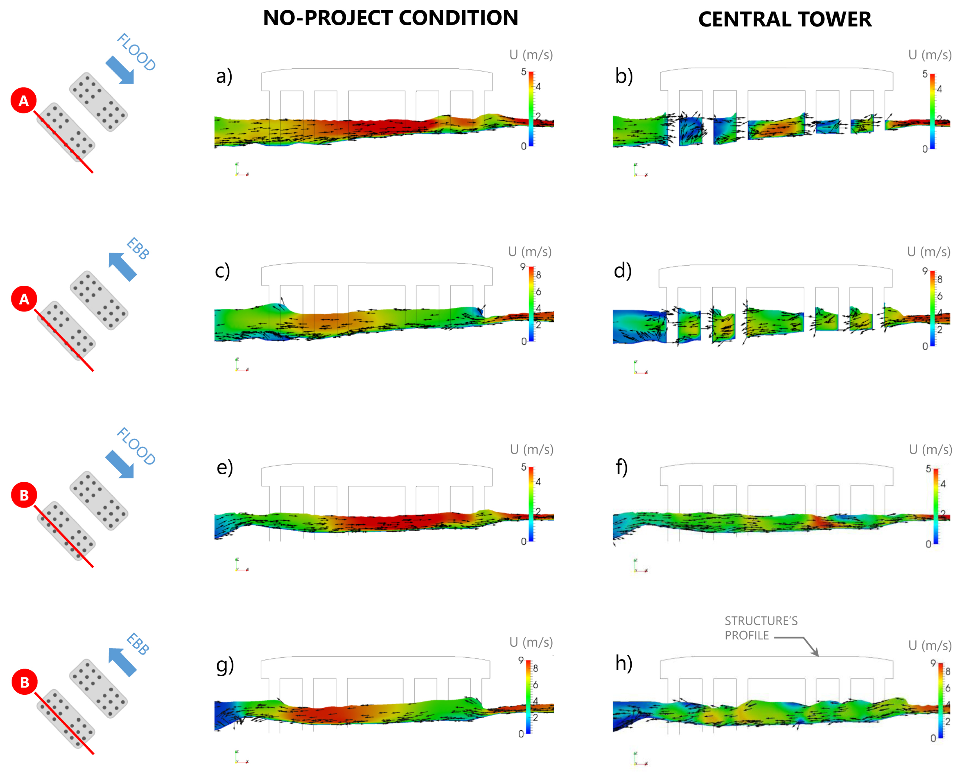
3.1. Flow Field
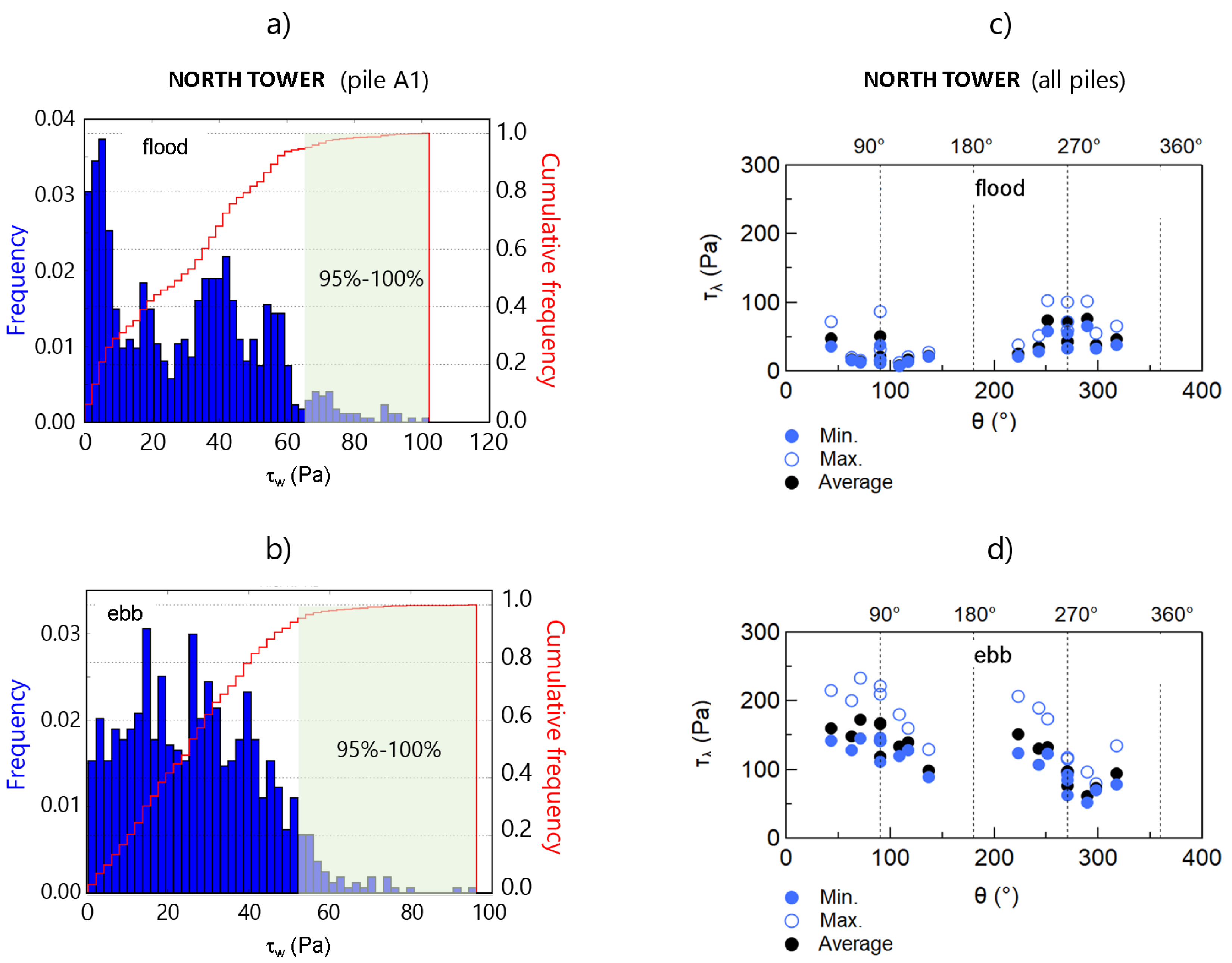
3.2. Shear Stress around Bridge Piers
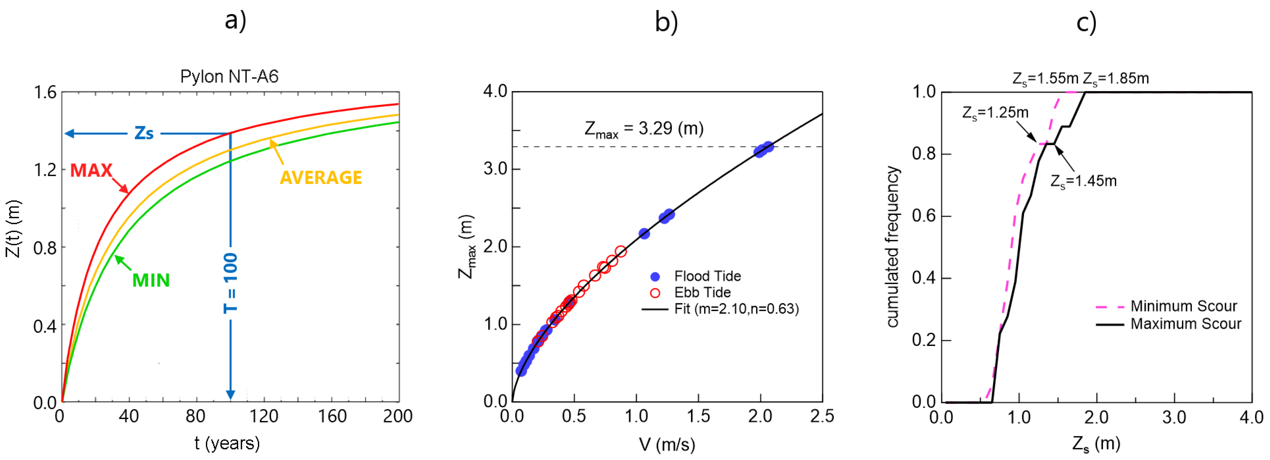
3.3. Erodibility and Scour Depth
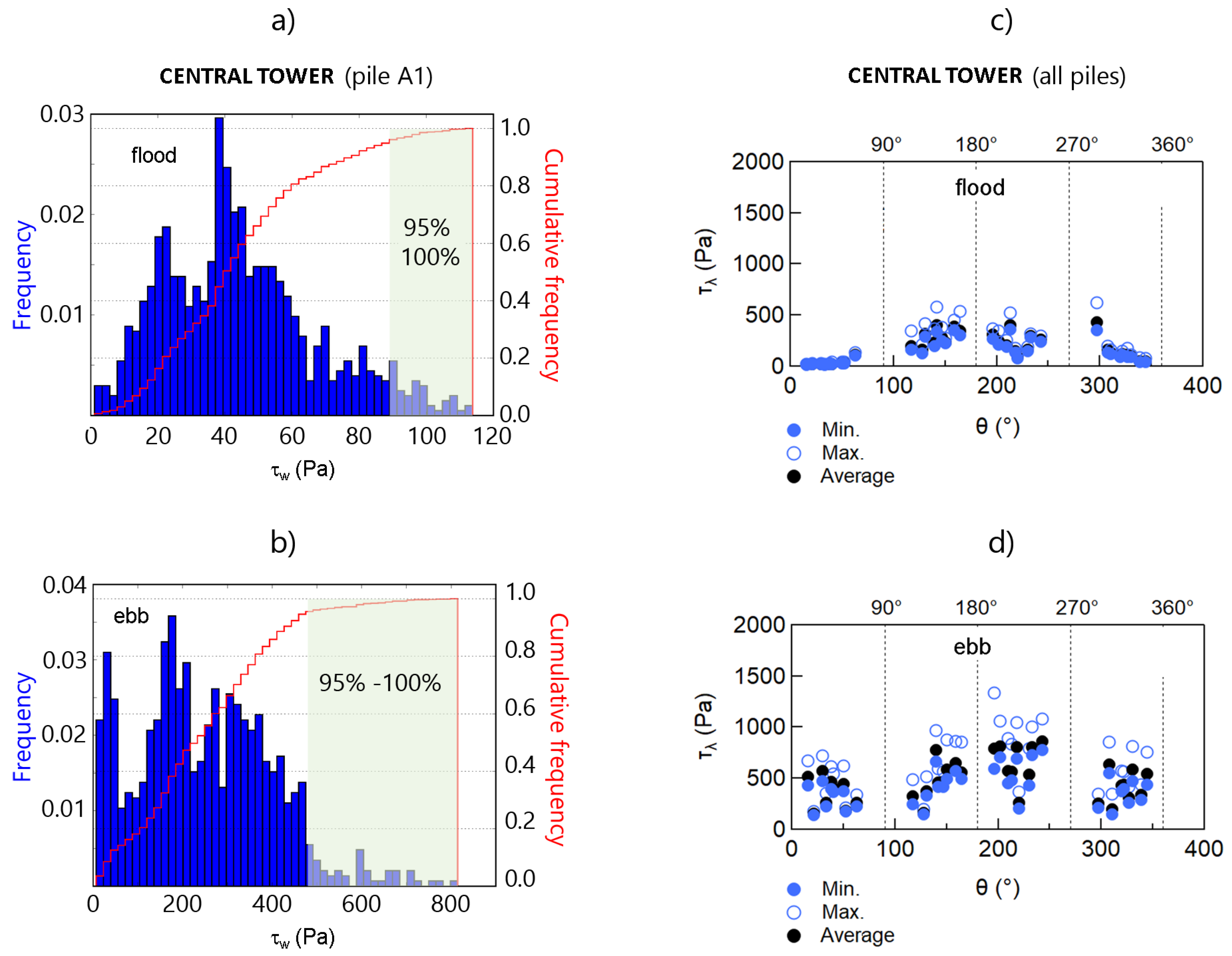
4. Results for Central Tower
4.1. Flow Field
4.2. Erodibility and Scour Depth
5. Discussion
5.1. About North Tower
5.2. About Central Tower
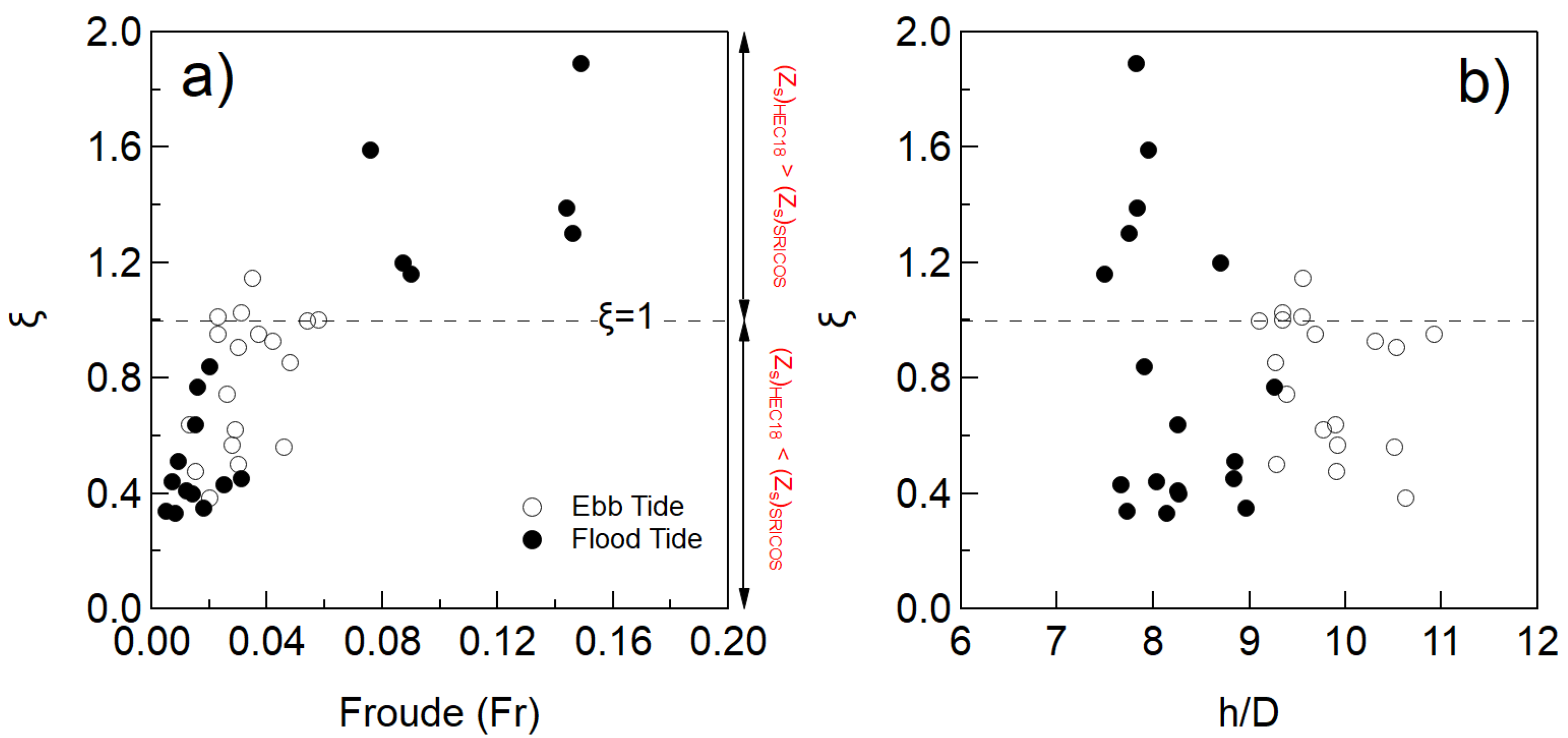
5.3. Design Value of Scour Depth
6. Conclusions
Author Contributions
Funding
Acknowledgments
Conflicts of Interest
References
- Syngros, K.; Dobry, R.; Leventis, G.E. Chacao Channel Bridge–the Design Challenges. In Proceedings of the International Conference on Case Histories in Geotechnical Engineering—Sixth International Conference on Case Histories in Geotechnical Engineering, Arlington, VA, USA, 11–16 August 2008. [Google Scholar]
- Forsberg, T. The challenge of constructing a bridge over the Chacao channel. In Proceedings of the Fourth Symposium on Strait Crossings, Bergen, Norway, 2–5 September 2001; p. 345. [Google Scholar]
- Forsberg, T. Multi-span suspension bridges. Int. J. Steel Struct. 2001, 1, 63–73. [Google Scholar]
- Valenzuela, M.A.; Márquez, M.A. Chacao Suspension Bridge: Tender and Technical Challenges. In Proceedings of the IABSE Symposium: Engineering for Progress, Nature and People, Madrid, Spain, 3–5 September 2014; pp. 2516–2523. [Google Scholar]
- Caceres, M.; Valle-Levinson, A.; Atkinson, L. Observations of cross-channel structure of flow in an energetic tidal channel. J. Geophys. Res. Ocean. 2003, 108, 968. [Google Scholar] [CrossRef]
- Cuatro; Cowi, I. Final Report—Engineering Study—Volumes 1 through 9. Technical Report, Ingeneria Cuatro/Cowi. 2001; (not available online). [Google Scholar]
- Aiken, C.M. Barotropic tides of the Chilean Inland Sea and their sensitivity to basin geometry. J. Geophys. Res. Ocean. 2008, 113, 4593. [Google Scholar] [CrossRef]
- Soto-Mardones, L.; Letelier, J.; Salinas, S.; Pinillas, E.; Belmar, J.P. Análisis de parámetros oceanográficos y atmosféricos del Seno de Reloncaví. Gayana (Concepción) 2009, 73, 141–155. [Google Scholar] [CrossRef]
- Warren, R.; Larsen, J.; Svendsen, H. Chacao Channel, an Extreme Application of MIKE 21; COWI Consulting Engineers and Planners AS: Lyngby, Denmark, 2007. [Google Scholar]
- Marín, V.H.; Campuzano, F.J. Un modelo hidrodinámico barotrópico para los fiordos australes de Chile entre los 41∘S y los 46∘S. Cienc. Tecnol. Del Mar 2008, 31, 125–136. [Google Scholar]
- Sepúlveda, I.; Winckler, P.; Cáceres, M. Hydrodynamic modeling of tidal currents and power extraction in Chacao Channel, Chile. In Proceedings of the 4th Annual Marine Renewable Energy Technical Conference, University of Massachusetts Dartmouth, North Dartmouth, MA, USA, 10 January 2013. [Google Scholar]
- De la Fuente, L.; Miguel, N.E. Hydrodynamic Modelling of Tidal Currents at Chacao Channel for a Preliminary Energy Resource Assessment. Master’s Thesis, Pontificia Universidad Católica de Chile, Escuela de Ingeniería, Santiago, Chile, 2012. [Google Scholar]
- Winckler, P.; Sepúlveda, I.; Aron, F.; Contreras-López, M. How do tides and tsunamis interact in a highly energetic channel? The case of canal Chacao, Chile. J. Geophys. Res. Ocean. 2017, 122, 9605–9624. [Google Scholar] [CrossRef]
- Peña, Á.; Valenzuela, M.; Márquez, M.; Pinto, H. Requerimientos geotécnicos mínimos para el diseño de fundaciones de puentes tradicionales y singulares: Puente Colgante Chacao. Rev. Construcción 2017, 16, 498–505. [Google Scholar] [CrossRef]
- Melville, B.W.; Coleman, S.E. Bridge Scour; Water Resources Publications LLC: Highlands Ranch, CO, USA, 2000. [Google Scholar]
- Ettema, R. Scour at Bridge Piers—Report No 216; Technical Report; University of Auckland: Auckland, New Zealand, 1980. [Google Scholar]
- Pizarro, A.; Manfreda, S.; Tubaldi, E. The science behind scour at bridge foundations: A review. Water 2020, 12, 374. [Google Scholar] [CrossRef]
- Shen, H.W.; Schneider, V.R.; Karaki, S. Local scour around bridge piers. J. Hydraul. Div. 1969, 95, 1919–1940. [Google Scholar] [CrossRef]
- Chiew, Y.M.; Melville, B.W. Local scour around bridge piers. J. Hydraul. Res. 1987, 25, 15–26. [Google Scholar] [CrossRef]
- May, R.; Ackers, J.; Kirby, A. Manual on Scour at Bridges and Other Hydraulic Structures; Ciria: London, UK, 2002; Volume 551. [Google Scholar]
- Annandale, G.W.; Kirsten, H.A. On the erodibility of rock and other earth materials. In Proceedings of the Hydraulic Engineering, Buffalo, NY, USA, 1–5 August 1994; pp. 68–72. [Google Scholar]
- Annandale, G. Erodibility. J. Hydraul. Res. 1995, 33, 471–494. [Google Scholar] [CrossRef]
- Annandale, G.W. Prediction of scour at bridge pier foundations founded on rock and other earth materials. Transp. Res. Rec. 2000, 1696, 67–70. [Google Scholar] [CrossRef]
- Annandale, G.; Smith, S. Calculation of Bridge Pier Scour Using the Erodibility Index Method; Technical Report; Colorado Department of Transportation: Denver, CO, USA, 2001.
- Annandale, G. Scour Technology: Mechanics and Engineering Practice; McGraw Hill Professional: New York, NY, USA, 2005. [Google Scholar]
- Annandale, G. Current state-of-the-art Rock Scouring Technology. In Geotechnics of Soil Erosion; ASCE: Denver, CO, USA, 2007; pp. 1–12. [Google Scholar]
- Keaton, J.R.; Mishra, S.K.; Clopper, P.E. Scour at Bridge Foundations on Rock; Transportation Research Board: Washington, DC, USA, 2012; Volume 717.
- Bloomquist, D. Erosion of Cored Samples for the Chacao Channel Bridge Project Chile, South America. Interim Report; Technical Report; GeoHazards Co.: Gainesville, FL, USA, 2017. [Google Scholar]
- Marine, S. Proyecto Puente Chacao, Ingeniería Básica. Estudio de Socavación y Erosión, CHB-CPC-DGN-RPT-0282; Technical Report; Skyring Marine Ltd.: Valparaíso, Chile, 2017. [Google Scholar]
- The OpenFOAM Foundation. 2014. Available online: https://scholar.google.ca/scholar?hl=zh-TW&as_sdt=0%2C5&q=The+OpenFOAM+Foundation.+2014.&btnG= (accessed on 11 November 2022).
- Pope, S.B. Turbulent Flows; Cambridge University Press: Cambridge, UK, 2000. [Google Scholar]
- Menter, F.R. Improved Two-Equation K-Omega Turbulence Models for Aerodynamic Flows—Technical Memorandum 103975; Technical Report; NASA Ames Research Center Moffett Field: Mountain View, CA, USA, 1992.
- Menter, F.R. Two-equation eddy-viscosity turbulence models for engineering applications. AIAA J. 1994, 32, 1598–1605. [Google Scholar] [CrossRef]
- Ahrens, J.; Geveci, B.; Law, C. Paraview: An End-user Tool for Large Data Visualization. 2005, Volume 717. Available online: https://datascience.dsscale.org/wp-content/uploads/2016/06/ParaView.pdf (accessed on 29 November 2022).
- Fluent, A. 12.0 User’s Guide; Ansys Inc.: Canonsburg, PA, USA, 2009; Volume 6, p. 552. [Google Scholar]
- Bloomquist, D.; Crowley, R. Enhancement of FDOT’s SERF Device and a Study of Erosion Rates of Rock, Sand, and Clay Mixtures Using FDOT’s RETA and SERF Equipment; Technical Report; Florida Department of Transportation: Tallahassee, FL, USA, 2010.
- Bloomquist, D.; Sheppard, D.M.; Schofield, S.; Crowley, R.W. The rotating erosion testing apparatus (RETA): A laboratory device for measuring erosion rates versus shear stresses of rock and cohesive materials. Geotech. Test. J. 2012, 35, 641–648. [Google Scholar] [CrossRef]
- Crowley, R. Development of FDOT SERF and RETA Design Equations for Coastal Scour When a Single Vertical Pile Is Subjected To Wave Attack; Technical Report; Florida Department of Transportation: Tallahassee, FL, USA, 2021.
- Castillo, L.G.; Carrillo, J.M. Scour, velocities and pressures evaluations produced by spillway and outlets of dam. Water 2016, 8, 68. [Google Scholar] [CrossRef]
- Bollaert, E.; Schleiss, A. Transient Water Pressures in Joints and Formation of Rock Scour Due to High-Velocity Jet Impact; Technical Report; Ecole Polytechnique Federale de Laussane, Platform of Hydraulic Constructions: Lausanne, Switzerland, 2002. [Google Scholar]
- Bollaert, E.; Schleiss, A. Scour of rock due to the impact of plunging high velocity jets Part I: A state-of-the-art review. J. Hydraul. Res. 2003, 41, 451–464. [Google Scholar] [CrossRef]
- Bollaert, E.; Schleiss, A. Scour of rock due to the impact of plunging high velocity jets Part II: Experimental results of dynamic pressures at pool bottoms and in one-and two-dimensional closed end rock joints. J. Hydraul. Res. 2003, 41, 465–480. [Google Scholar] [CrossRef]
- Jalili Kashtiban, Y.; Saeidi, A.; Farinas, M.I.; Quirion, M. A Review on Existing Methods to Assess Hydraulic Erodibility Downstream of Dam Spillways. Water 2021, 13, 3205. [Google Scholar] [CrossRef]
- Moore, J. The characterization of rock for hydraulic erodibility. In Technical Release; USDA: Washington, DC, USA, 1991; Volume 78. [Google Scholar]
- Moore, J.S.; Temple, D.M.; Kirsten, H.A. Headcut advance threshold in earth spillways. Bull. Assoc. Eng. Geol. (United States) 1994, 31, 7231905. [Google Scholar]
- Kirsten, H. A classification system for excavating in natural materials. Civ. Eng. Siviele Ingenieurswese 1982, 1982, 293–308. [Google Scholar]
- Kirsten, H. Case histories of groundmass characterization for excavatability. In Rock Classification Systems for Engineering Purposes; ASTM International: West Conshohocken, PA, USA, 1988. [Google Scholar]
- Arneson, L.; Zevenbergen, L.; Lagasse, P.; Clopper, P. Evaluating Scour at Bridges; Technical Report; U.S. Department of Transportation, Federal Highway Administration: Washington, DC, USA, 2012.
- Deere, D. The rock quality designation (RQD) index in practice. In Rock Classification Systems for Engineering Purposes; ASTM International: West Conshohocken, PA, USA, 1988. [Google Scholar]
- Mandl, G. Rock Joints; Springer: Berlin/Heidelberg, Germnay, 2005. [Google Scholar]
- Barton, N. Rock mass classification and tunnel reinforcement selection using the Q-system. In Rock Classification Systems for Engineering Purposes; ASTM International: West Conshohocken, PA, USA, 1988. [Google Scholar]
- Yang, C.T. Incipient motion and sediment transport. J. Hydraul. Div. 1973, 99, 1679–1704. [Google Scholar] [CrossRef]
- Chow, V. Open-Channel Hydraulics, Classical Textbook Reissue; Mc-Graw Hill: New York, NY, USA, 1988. [Google Scholar]
- Sumer, B.; Christiansen, N.; Fredsoe, J. Time scale of scour around a vertical pile. In Proceedings of the Second International Offshore and Polar Engineering Conference, San Francisco, CA, USA, 14–19 June 1992. [Google Scholar]
- Gazi, A.H.; Afzal, M.S.; Dey, S. Scour around piers under waves: Current status of research and its future prospect. Water 2019, 11, 2212. [Google Scholar] [CrossRef]
- Briaud, J.L.; Ting, F.; Chen, H.; Cao, Y.; Han, S.; Kwak, K. Erosion function apparatus for scour rate predictions. J. Geotech. Geoenvironmental Eng. 2001, 127, 105–113. [Google Scholar] [CrossRef]
- Briaud, J.; Chen, H.; Kwak, K.; Han, S.; Ting, F. Multiflood and multilayer method for scour rate prediction at bridge piers. J. Geotech. Geoenviron. Eng. 2001, 127, 114–125. [Google Scholar] [CrossRef]
- Briaud, J.L. The Sricos-EFA Method. In Current Practices and Future Trends in Deep Foundations; American Society of Civil Engineers: Reston, VA, USA, 2004; pp. 348–360. [Google Scholar]
- Briaud, J.L.; Chen, H.C. SRICOS-erosion function apparatus method: An overview of its measurement of scour depth. In Proceedings of the 6th International Bridge Engineering Conference: Reliability, Security, and Sustainability in Bridge Engineering, Boston, MA, USA, 17–20 July 2005; pp. 525–529. [Google Scholar]
- Kwak, K.; Briaud, J.L.; Cao, Y.; Chung, M.; Hunt, B.; Davis, S. Pier scour at Woodrow Wilson Bridge and SRICOS method. In Proceedings of the First International Conference on Scour of Foundations, College Station, TX, USA, 17–20 November 2002; pp. 227–241. [Google Scholar]
- Kwak, K.S.; Briaud, J.L. Case study: An analysis of pier scour using the SRICOS method. KSCE J. Civ. Eng. 2002, 6, 243–253. [Google Scholar] [CrossRef]
- Briaud, J.; Chen, H.C.; Li, Y.; Nurtjahyo, P.; Wang, J. SRICOS-EFA method for contraction scour in fine-grained soils. J. Geotech. Geoenviron. Eng. 2005, 131, 1283–1294. [Google Scholar] [CrossRef]
- Briaud, J.L.; Ting, F.C.; Chen, H.; Gudavalli, R.; Perugu, S.; Wei, G. SRICOS: Prediction of scour rate in cohesive soils at bridge piers. J. Geotech. Geoenviron. Eng. 1999, 125, 237–246. [Google Scholar] [CrossRef]
- Ting, F.C.K.; Jones, A.L.; Larsen, R.J. Evaluation of SRICOS Method on Cohesive Soils in South Dakota; Technical Report; Mountain-Plains Consortium: Brookings, SD, USA, 2010. [Google Scholar]
- Richardson, E.; Davis, S. Evaluating Scour at Bridges; Technical Report; Federal Highway Administration. Office of Bridge Technology: Washington, DC, USA, 2001.
- Shan, H.; Kilgore, R.; Shen, J.; Kerenyi, K. Updating HEC-18 Pier Scour Equations for Noncohesive Soils; Technical Report; United States. Federal Highway Administration. Office of Infrastructure Research and Development: Georgetown, TX, USA, 2016.
- Mondal, M.S. Local Scour at Complex Bridge Piers in Bangladesh Rivers: Reflections from a Large Study. Water 2022, 14, 2405. [Google Scholar] [CrossRef]
- Comodromos, E.M.; Anagnostopoulos, C.T.; Georgiadis, M.K. Numerical assessment of axial pile group response based on load test. Comput. Geotech. 2003, 30, 505–515. [Google Scholar] [CrossRef]
- Briaud, J.L.; Hunt, B. Bridge scour and the structural engineer. Structure 2006, 2006, 58–61. [Google Scholar]


| Description | Item | Central Tower (CT) | North Tower (NT) |
|---|---|---|---|
| Grid Stats | Mesh software | SnappyHexMesh | SnappyHexMesh |
| # of Points | 2,020,283 | 2,171,168 | |
| # of Faces | 5,109,534 | 5,447,175 | |
| Internal | 4,722,233 | 4,977,149 | |
| # of Cells | 1,565,737 | 1,656,988 | |
| Skewness (max) | 3.72 | 4.13 | |
| Solver/Numerics | Internal solver | InterFoam | InterFoam |
| (incompressible/biphase) | (incompressible/biphase) | ||
| Continuity link with pressure | PIMPLE algorithm | PIMPLE algorithm | |
| Interpolation advection scheme (U) | Linear Upwind | Linear Upwind | |
| Interpolation advection scheme () | Van Leer | Van Leer | |
| Linear solvers for Prgh | GAMG /PCG | GAMG /PCG | |
| (w/preconditioner) | (w/preconditioner) | ||
| Linear solvers for | SmoothSolver | SmoothSolver | |
| GaussSeidel | GaussSeidel | ||
| Turbulence Treatment | Primary aproximation | RANS | RANS |
| Turbulence closure model | kOmegaSST | kOmegaSST | |
| Boundary Conditions | Wave2Foam | Wave2Foam | |
| w/relaxation zone | w/relaxation zone | ||
| Initial Conditions | Velocity (U) | 0 | 0 |
| Pressure (P) | Hydrostatic P. by sea lvl. | Hydrostatic P. by sea lvl. | |
| Air-water by cell z coord. | Air-water by cell z coord. |
| Velocity | Free Surface | ||||
|---|---|---|---|---|---|
| (m/s) | (m.a.s.l.) | ||||
| Site | Scenario | NW | SE | NW | SE |
| North Tower | Flood-Tide | 2.38 | 2.27 | −2.32 (1) | −2.32 |
| North Tower | Ebb-Tide | −2.69 (2) | −2.66 | 1.60 | 1.63 |
| Central Tower | Flood-Tide | 3.60 | 2.48 | −1.81 | −1.87 |
| Central Tower | Ebb-Tide | −3.25 | −2.87 | 1.70 | 1.94 |
| Sample | Run | T | ||||
|---|---|---|---|---|---|---|
| (N·mm) | (hr.) | (g) | (Pa) | (mm/year) | ||
| TN1 | 1 | 15 | 13.2 | 1.49 | 20.88 | 18.10 |
| 2 | 15 | 35.5 | 2.17 | 20.88 | 9.80 | |
| 3 | 30 | 6.2 | 0.00 | 41.76 | 0.00 | |
| 4 | 30 | 19.3 | 0.68 | 41.76 | 5.60 | |
| 5 | 45 | 6.0 | 0.38 | 62.63 | 10.20 | |
| 6 | 60 | 6.0 | 0.38 | 83.51 | 10.20 | |
| TN2 | 1 | 40 | 17.3 | 1.87 | 78.47 | 32.74 |
| 2 | 30 | 26.0 | 0.79 | 58.86 | 9.22 | |
| 3 | 20 | 34.0 | 0.58 | 39.24 | 5.18 | |
| 4 | 15 | 11.0 | 0.23 | 29.43 | 6.35 | |
| 5 | 50 | 22.0 | 1.11 | 98.09 | 15.31 | |
| TN3 | 1 | 2 | 20.0 | 3.18 | 5.77 | 32.60 |
| 2 | 20 | 7.3 | 0.49 | 52.46 | 13.90 | |
| 3 | 30 | 8.0 | 0.62 | 78.69 | 15.90 | |
| Min. | 6.0 | 5.77 | 0.00 | |||
| Max. | 35.5 | 98.09 | 32.74 | |||
| Average | 16.6 | 50.89 | 13.22 |
| Sample | Run | T | ||||
|---|---|---|---|---|---|---|
| (N·mm) | (hr.) | (g) | (Pa) | (mm/year) | ||
| RR1 | 1 | 15 | 30.0 | 0.00 | 21.01 | 0.00 |
| 2 | 25 | 66.5 | 0.00 | 35.02 | 0.00 | |
| 3 | 50 | 99.0 | 0.00 | 70.05 | 0.00 | |
| RR2 | 1 | 40 | 14.0 | 2.16 | 113.52 | 402.97 |
| 2 | 20 | 21.0 | 0.25 | 56.76 | 46.64 | |
| 3 | 10 | 72.0 | 0.35 | 28.38 | 65.30 | |
| 4 | 30 | 48.0 | 0.46 | 85.14 | 85.82 | |
| RR3 | 1 | 40 | 14.0 | 2.16 | 113.52 | 402.97 |
| 2 | 200 | 1.4 | 0.02 | 294.73 | 3.90 | |
| 3 | 250 | 1.1 | 0.01 | 368.41 | 1.90 | |
| RR4 | 1 | 50 | 137.0 | 0.00 | 99.44 | 0.00 |
| RR5 | 1 | 60 | 149.5 | 0.00 | 90.63 | 0.00 |
| Min. | 1.1 | 21.0 | 0.00 | |||
| Max. | 149.5 | 368.4 | 402.97 | |||
| Average | 54.5 | 114.7 | 84.12 |
| Symbol | Description | Value | Comment |
|---|---|---|---|
| Mass strength number | 8.39 | It considers information extracted | |
| from geotechnical test (in MPa) | |||
| Particle size number | 19.04 | ||
| Average joint spacing (along x) | 1.00 | It considers a mean spacing | |
| =, where 6 m | |||
| Average joint spacing (along y) | 1.00 | ||
| Average joint spacing (along z) | 1.00 | ||
| d | Mean diameter of blocs | 1.00 | Measured in (m) |
| = | 6.00 | ||
| Rock quality | 95.20 | This parameter usually ranges | |
| from 0 to 100 | |||
| Joint set number | 5.00 | Considering very fractured | |
| rock, suggested by [25,27] | |||
| Shear strength number | 0.10 | ||
| Joint roughness | 1.00 | It assumes that joints remain | |
| open during rock’s scour | |||
| Joint alteration | 10.00 | It considers rock void spaces | |
| filled with strongly consolidated | |||
| cohesive materials, with or without | |||
| crushed rocks | |||
| Ground structure number | 0.73 | Value suggested by [27] | |
| K | Erodibility index | 11.66 | |
| P | Threshold Power | 6.31 | kWatt·m−2 |
Disclaimer/Publisher’s Note: The statements, opinions and data contained in all publications are solely those of the individual author(s) and contributor(s) and not of MDPI and/or the editor(s). MDPI and/or the editor(s) disclaim responsibility for any injury to people or property resulting from any ideas, methods, instructions or products referred to in the content. |
© 2023 by the authors. Licensee MDPI, Basel, Switzerland. This article is an open access article distributed under the terms and conditions of the Creative Commons Attribution (CC BY) license (https://creativecommons.org/licenses/by/4.0/).
Share and Cite
Martinez, F.; Winckler, P.; Zamorano, L.; Landeta, F. Bridge Pier Scour in Complex Environments: The Case of Chacao Channel in Chile. Water 2023, 15, 296. https://doi.org/10.3390/w15020296
Martinez F, Winckler P, Zamorano L, Landeta F. Bridge Pier Scour in Complex Environments: The Case of Chacao Channel in Chile. Water. 2023; 15(2):296. https://doi.org/10.3390/w15020296
Chicago/Turabian StyleMartinez, Francisco, Patricio Winckler, Luis Zamorano, and Fernando Landeta. 2023. "Bridge Pier Scour in Complex Environments: The Case of Chacao Channel in Chile" Water 15, no. 2: 296. https://doi.org/10.3390/w15020296
APA StyleMartinez, F., Winckler, P., Zamorano, L., & Landeta, F. (2023). Bridge Pier Scour in Complex Environments: The Case of Chacao Channel in Chile. Water, 15(2), 296. https://doi.org/10.3390/w15020296