Characterization of Relative Movements between Blocks Observed in a Concrete Dam and Definition of Thresholds for Novelty Identification Based on Machine Learning Models

Abstract

Dam surveillance activities are based on observing the structural behaviour and interpreting the past behaviour supported by the knowledge of the main loads. For day-to-day activities, data-driven models are usually adopted. Most applications consider regression models for the analysis of horizontal displacements recorded in pendulums. Traditional regression models are not commonly applied to the analysis of relative movements between blocks due to the non-linearities related to the simultaneity of hydrostatic and thermal effects. A new application of a multilayer perceptron neural network model is proposed to interpret the relative movements between blocks measured hourly in a concrete dam under exploitation. A new methodology is proposed for threshold definition related to novelty identification, taking into account the evolution of the records over time and the simultaneity of the structural responses measured in the dam under study. The results obtained through the case study showed the ability of the methodology presented in this work to characterize the relative movement between blocks and for the identification of novelties in the dam behaviour.

1. Introduction

Structural monitoring involves observing a phenomenon or event and its impact on the structure. The purpose of the analysis and interpretation of the measurements gathered during an inspection is to enhance the conceptual understanding of the dam’s behaviour and aims to define, based on better parameters, eventual models. Once a model is built, the dam’s condition assessment is based on test hypotheses and scenario simulations supported by the monitoring data and the prediction of the structural behaviour in space and time. The procedure of providing information for assessing the dam’s structural condition is a form of critical analysis capable of reducing the intrinsic uncertainty related to the dam’s behaviour.

The assessment of the dam’s condition based on the information provided by the monitoring system is possible if the information is updated. Any abnormal behaviour can be readily identified, allowing for the implementation of an appropriate intervention or prevention measures. The assessment of the structural behaviour of the dam and its condition must be performed for each dam independently, even for dams of the same type, since they are influenced by several aspects, such as the heterogeneities in the dam’s foundation and the surrounding areas of the dam or the different loads (as a consequence of environmental or operational conditions) that the structure receives. For each concrete dam, different models can be used according to each purpose, to the existing knowledge about the actual structural behaviour, and the quality of information available for the characterization of the structure’s behaviour. The selection of the conceptual model to be used for dam surveillance activities must take into account: (i) the purpose of the analysis (safety assessment, prediction of deformations, interpretation of the recorded data from the monitoring system, or analysis of an accident or abnormal behaviour), (ii) the identification of the key factors of the physical problem, and (iii) the available geological and geotechnical information.

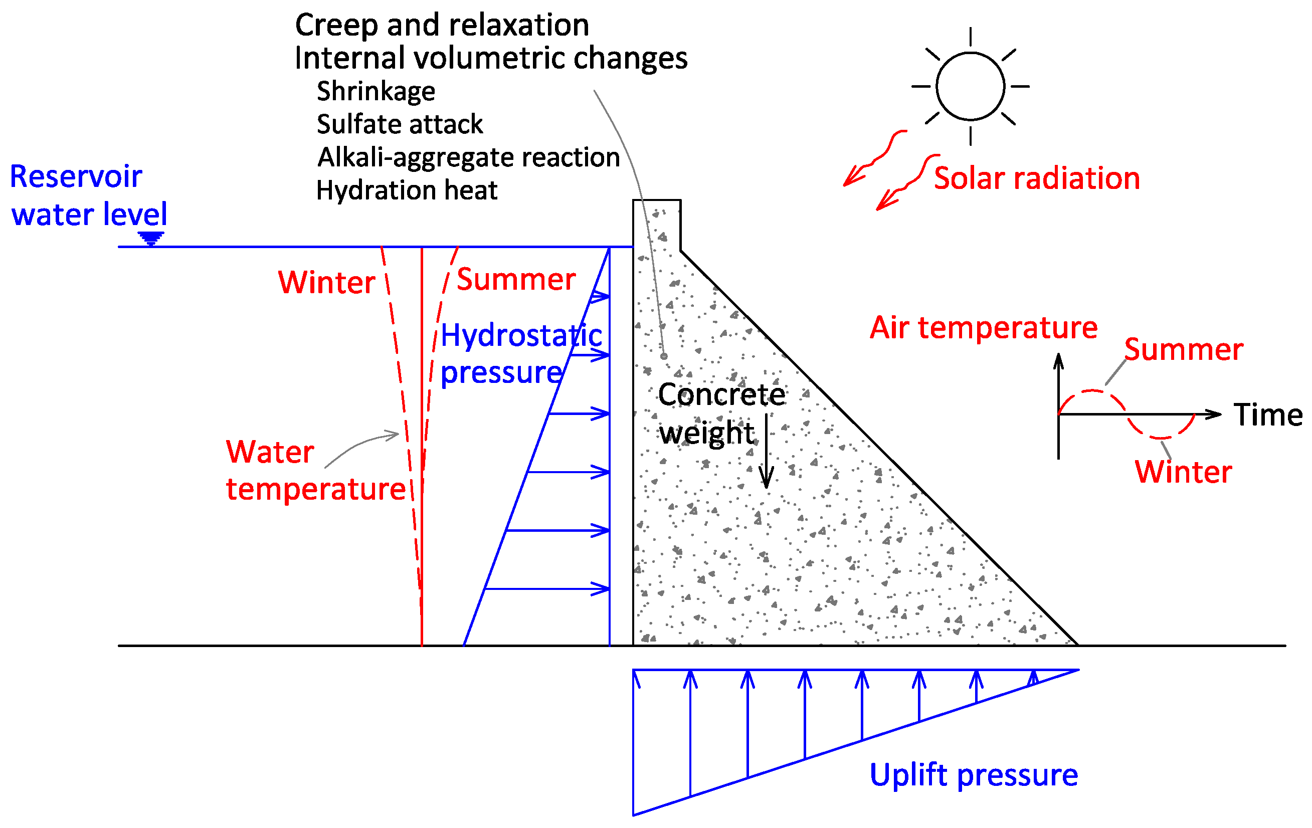
During a dam’s life, the performance and safety conditions are under continuous assessment due to the potential failure scenarios identified during the design phase and due to the other scenarios “suggested” by the observed behaviour through the analysis of relevant parameters (such as water level and temperature variations, among other things), as seen in Figure 1. Typically, these parameters will describe the loads or operating conditions to which the system is subjected, the materials of the structure, the materials of the structure’s foundations, and the structural response of the dam [1]. Thus, visual inspections and measurements collected by the structural monitoring system are fundamental for safety control activities. The main physical quantities measured through the monitoring system are seepage and leakage, uplift pressure, horizontal displacements, vertical displacements, relative displacements between blocks (contraction joint movements), and relative displacements in the rock mass foundation. The interpretation of the observed values is usually based on knowledge related to the physical and chemical phenomena that govern the structure and, whenever possible, is based on deterministic or data-based models. For decision-making, deterministic models are preferred, while in day-to-day activities, data-based models are the most commonly used.

The most common approaches for data-based models are the HST (hydrostatic, seasonal, time) and the HTT (hydrostatic, thermal, time) models, in which the effects of hydrostatic pressure, temperature, and time are considered additive effects, and their separation is valid [1,2,3,4,5]. The hydrostatic pressure is usually considered a polynomial function of the water height. However, in addition to the pressure from the water, dams in cold regions may be exposed to loads from an ice sheet [6]. The time effect is represented by polynomial functions or by functions of another type (exponential or s-shaped). The thermal effect is considered differently in each approach. In the HST approach, the temperature effect is represented by sinusoidal functions with a one-year period, which are a function of the day of the year only. In the HTT approach, the temperature effect is a function of the measured temperatures. A large number of publications about HST and HTT models can be consulted in the literature [1,2,3,4,5,6,7,8,9,10,11,12,13,14,15].

Multiple linear regression is one of the most commonly used data-based models [3], showing good performance, mainly for case studies related to the prediction of horizontal and vertical displacements observed on a dam body. On the other hand, new models based on machine learning have been studied and published for about a decade with positive results; these are proposed mainly for the analysis of displacements. Proposed machine learning models could differ in their approach and advantages; such is the case of artificial neural network (NN) models, which principally allow the identification of non-linear relationships between the input quantities, if any. One main aspect to take into account in the case of NN models is that suitable generalization criteria, such as cross-validation criteria, must be adopted to avoid overfitting [5].

There are quantities, such as seepage, uplift pressure, and relative movements between blocks, in which regression models could be used with special care since the separation of effects may not be valid. For example, the behaviour of contraction joints depends on the state of stress installed. The variation observed differs for “open” or “closed” joints. Joint opening and closure are governed by normal stress criteria. The non-linear behaviour presented by the contraction joints can be explained by the non-resistance of the contraction joints to tension. As referred to by Hariri and Kianoush, modelling the joints (contraction, peripheral and lift joints) has an important role in both the static and the seismic analysis of concrete arch dams [16]. Some authors developed a non-linear joint element to represent the behaviour of vertical contraction joints in concrete dams [16,17,18,19,20,21]. The current knowledge in the field of machine learning allows the proper interpretation and prediction of these quantities, including anomaly detection [22,23], knowledge that is expected to grow in the following years.

The definition of thresholds for novelty identification related to movements in contraction joints is a natural step in the safety control activities of dams. For the identification of damage or gross measurement errors, the limits can be based on deterministic models or even on the maximum values observed in the dam life history affected by a multiplicative factor. However, identifying novelties earlier could be based on narrower limits resulting from data-based models. Nowadays, the definition of thresholds has been mainly based on considering a multiplicative factor associated with the standard deviation of residuals (the part not explained by the model adopted). This analysis allows the point-to-point identification of values that exceed established limits without any temporal or multidimensional context. Thus, two methodologies for threshold definition are presented in this work, one complementary to the traditional approach that can be used for the identification of novelties in a temporal context through the consideration of moving averages and the moving standard deviation of the residuals, and another, in a multidimensional context, through the use of the density-based spatial clustering of applications with noise (DBSCAN) method [24].

The methodology proposed is presented in Section 2. The case study, a concrete dam under exploitation, and the relative movements between blocks registered by the measurements of an automated monitoring system are described in Section 3. The results and final remarks are presented in Section 4 and Section 5.

2. Methodology Proposed for the Characterization of Relative Movements between Blocks and for Threshold Definition for Novelty Identification

2.1. Methodology

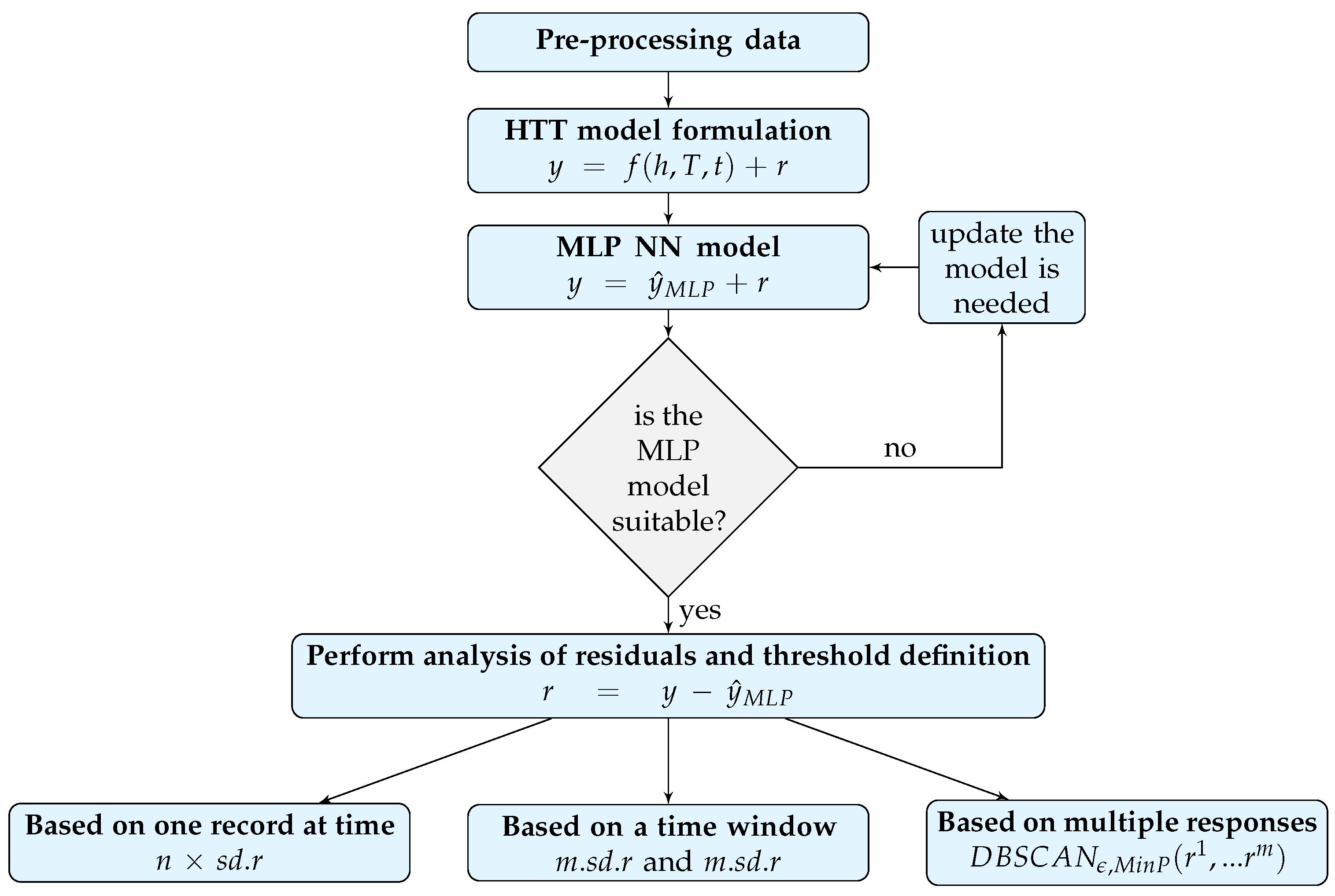
The priority for any threshold definition process is an adequate data-based model with a proper approach. The HTT approach was chosen in this study because of the daily variation observed in the quantity under study (relative movement between blocks). Enough information was obtained from the dam body’s thermometer and water level measurement devices. Regarding the machine learning method adopted, the authors selected the MLP-NN method. The methodology for the definitions of thresholds based on the residuals of the data-based models developed from the past history of the records (relative movements between blocks in the case study) is detailed ahead:

• The adoption of the HTT formulation for the development of the prediction model requires the selection of the main physical quantities to be used. The water height and the concrete dam body temperature variations are the selected main inputs in the proposed model.
• The separation of effects in the analysis of the relative movements between blocks may not be verified, so a model capable of mapping the interaction between the inputs is recommended. In this sense, an MLP-NN model was found to be suitable. Once the MLP-NN model is obtained, the influence of the main loads on the responses, as well as the analysis of the residuals, r, can be analysed.
• The definition of thresholds for novelty identification based on the residuals can be defined: (i) based on one record at a time, (ii) based on a time window of records, (iii) and based on the simultaneity of the responses measured, as shown below.
• A threshold definition based on one record at a time is the most used type of threshold in dam engineering and consists of the adoption of a multiplier n applied to the standard deviation of the residuals, $sd.r.$, as follows: $n\times sd.r.$ Values of n equal to 3 and 4 correspond to a confidence level of 99.73% and 99.99%, respectively, since residuals are assumed to follow a Gaussian distribution.
• A threshold definition based on a time window of records of one physical quantity is based on the moving average of the residuals, $m.a.r.$, and the moving standard deviation of the residuals, $m.sd.r.$, adopting a time window of records over time. The size of the time window may depend on the case under study.
• A threshold definition based on the simultaneity of the responses measured allows the identification of novelties related to a cluster of data (with m features) related to the m quantities considered in the analysis. $DBSCAN$ is a method suitable for this approach, in which it is necessary to adopt, as an initial step, suitable values for Epsilon distance, $ϵ$ and MinPoints, $MinP$ (Section 2.4). Hence, the residuals related to several physical quantities $(r^1,\dots r^m)$, with m being the number of features measured simultaneously, are assessed to define clusters of the ones that present a behaviour far from that of the remaining data.

The proposed flowchart for the interpretation of the relative movements between blocks and for the operational threshold definition is presented in Figure 2.

The theoretical background related to the MLP-NN algorithm, the moving average, the moving standard deviation of the residuals, and the DBSCAN method are presented in the following subsections.

2.2. Multilayer Perceptron Neural Network Algorithm

Artificial neural networks have caught the attention of the scientific community since the 1990s [25] due to their ability to learn the pattern of structural behaviour in large infrastructures with a good capacity for generalization [5,14,26,27,28,29,30,31]. A NN computes a function of the inputs by propagating the computed values from the input neurons to the output neurons using different weights as an intermediate parameter [26]. A multilayer perceptron neural network is a feed-forward algorithm with neurons arranged in layers. 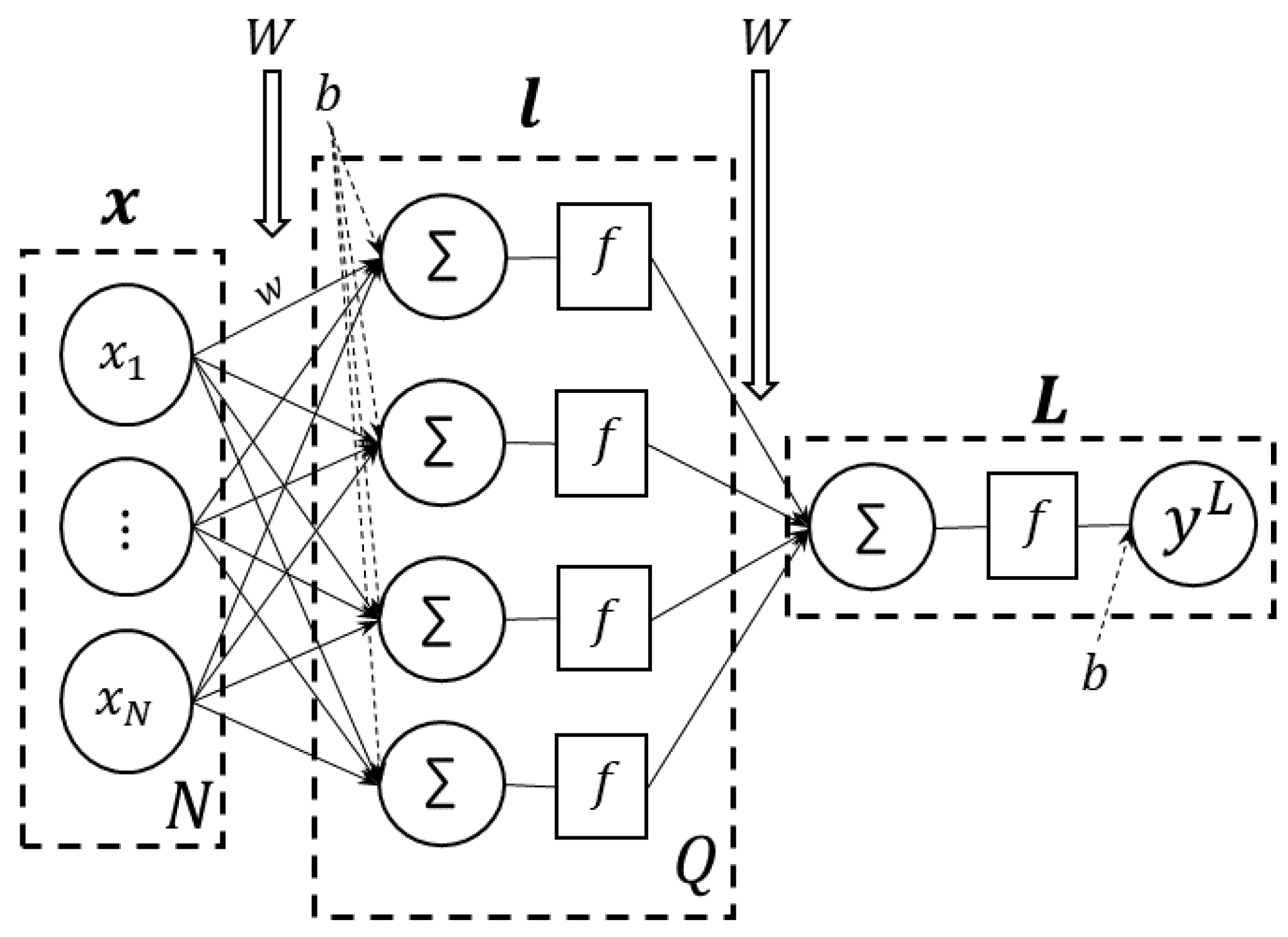It is the most widely used model for cognitive tasks such as pattern recognition and function approximation [5]. The specific architecture of feed-forward networks assumes that all nodes in one layer are connected to those of the next layer. The input layer transmits the data to the output layer going through a set of hidden layers that perform computations that include refining the weights between neurons over many input-output pairs to provide more accurate predictions.

The MLP-NN (Figure 3) learns by an iterative weight adjustment process that enables the correct learning using the training data so that, in a testing phase, it predicts the unknown data. Those weights w are located in each connection between the input layer x with N neurons and the hidden layer l with Q. The first layer receives the inputs, and the last layer produces the outputs. The middle layer is called the hidden layer. Within it, the information is constantly feed-forwarded from one layer to the next one having two associated values: the input value and the weight. In mathematics and programming, weights are shown in a matrix format W, where the number of columns contains the input dimensions (input values and weights), and the number of rows contains the output dimensions (hidden layer neurons Q). Another weight associated with the network is the bias b. Bias is attached to every layer in the network except for the input layer and carries neurons that try to account for unforeseen or non-observable factors. Activation functions are applied to each of the neurons in the hidden layer. The activation function will map the linear combinations of the inputs and weights to the following layer, in the case presented in Figure 3 from the input layer to the hidden layer and, in a further step, to the output layer of network L.

For regression problems, such as those found in the framework of SHM, the activation functions must be differentiable so that any non-linear models built from them can be derived with respect to their weights [32]. In this case, the activation function from the input layer to the hidden layer f can be the logistic sigmoid or the hyperbolic tangent function. The activation function from the hidden layer to the output layer g is a linear function.

2.3. Time-Window Threshold Definition Based on the Moving Average and Moving Standard Deviation of the Residuals

The detection of any deviation not identified by the prediction model between the observed and predicted data, is one of the main objectives of the residual analysis. A moving average control chart of the residuals ($m.a.r.$) is a type of memory control chart based on an unweighted moving average, and it is defined as

$${m.a.r.}_i=\frac{m.sum.r{.}_i}{w}=\frac{{\sum }_{j=i-w+1}^i{r}_j}{w},i\ge w$$

(1)

where w is the width of the moving average at time i.

In order to describe the dispersion of residuals, the $m.sd.r.$ is also presented in order to know how much the residuals vary or how spread they are along time, being defined as

$$m.sd.r{.}_i=\sqrt{\frac{1}{w-1}\sum _{j=i-w+1}^i{(x_j-{\overline{x}}_{jtoi})}^2}$$

(2)

For these periods, the average of all observations within a time window of w size up to time i defines the moving average. Four different $m.a.r.$, related to 6, 12, 24, and 168 records, correspondent to a quarter, a half, an entire day, and a week, are potential options to be considered in this type of study. However, only the results of a $m.a.r.$ and $m.sd.r.$ with a time window of one day and a time step of one hour are presented in this work.

Once the $m.a.r.$ and the $m.sd.r.$ are established, the definition of a baseline of the structural behaviour under normal conditions is possible. The $m.a.r.$, in this sense, allows the identification of extreme values and trends along a time period. The $m.sd.r.$ allows the identification of any increment of variability and/or randomness along the same time period. Those changes might suggest novelty.

2.4. Multivariate Threshold Definition Based on DBSCAN Algorithm

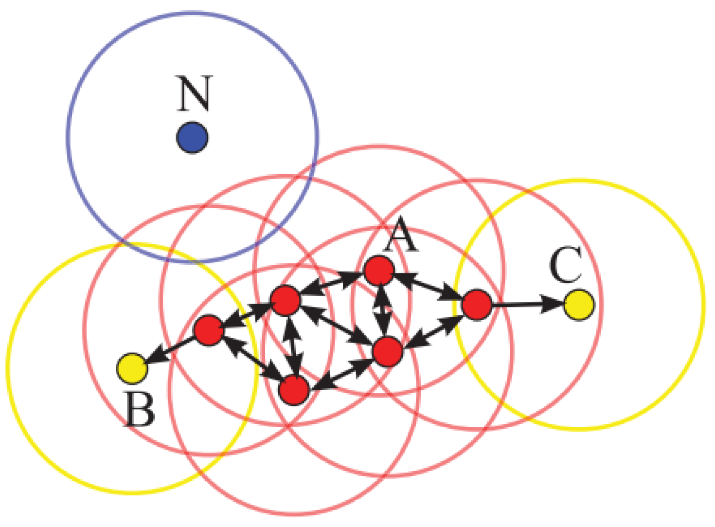
Density-based spatial clustering of applications with noise is a clustering algorithm proposed by Ester et al. [24]. It searches for “core objects”, points that contain a minimum of observations (MinPoints) within its neighbourhood (defined by an epsilon radius), including the core point itself. If a point is found outside of any of the core object’s neighborhood, it is considered noise [33]. Border points are points within reach of a core object without the minimum points in their neighbourhood to be considered core objects themselves (Figure 4). DBSCAN is known to be able to discover clusters with shapes other than linear and be robust enough to handle outliers and noise.

The clusters are created as follows: after uncovering a core object (i.e., a point with a high density of neighbours according to the parameters), DBSCAN starts a cluster with it and all its neighbours. All points within the Epsilon distance of the neighbours are then added to the cluster. This process continues until there are no more points within the distance. All the points that do not belong to a neighbourhood (i.e., to a cluster) are considered noise or outliers.

3. Case Study

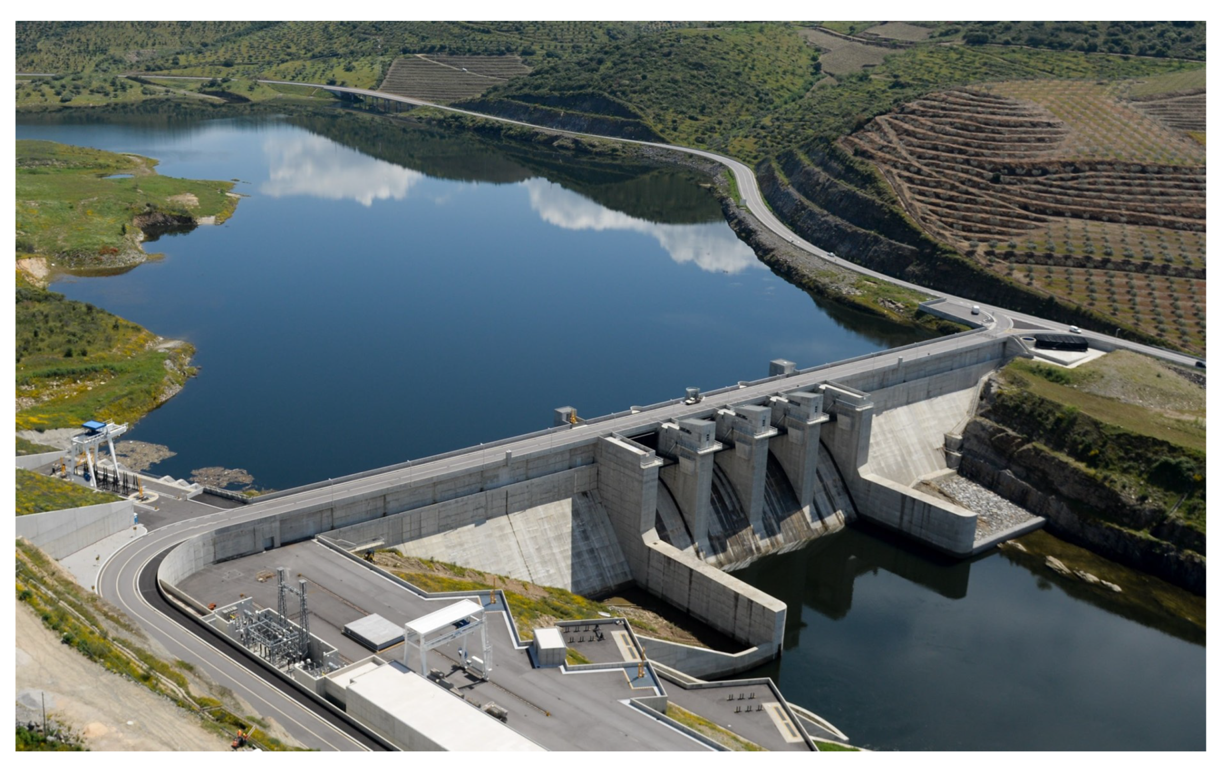
3.1. The Feiticeiro Dam

The hydroelectric development of Baixo Sabor is composed of two schemes. The upstream scheme (termed the Baixo Sabor dam) is 12.6 km away from the Sabor river mouth. The downstream scheme (termed the Feiticeiro dam, Figure 5) is about 3.3 km far from the mouth of the Sabor river [35]. The Feiticeiro dam comprises a concrete gravity dam with an overflow-controlled spillway and a downstream stilling basin. The dam is 45 m high and has a crest length of 315 m, which is divided into twenty-two blocks. The total concrete volume is equal to 130,000 m${}^3$.

In accordance with the best technical practices, the monitoring system of the Feiticeiro dam aims at the evaluation of the loads, the characterisation of the rheological, thermal and hydraulic properties of the materials, and the evaluation of the dam’s structural response. The monitoring system of the Feiticeiro dam consists of several devices that make it possible to measure quantities such as the concrete and air temperatures, reservoir water level, seepage and leakage, displacements in the dam and in its foundation, joint movements, strains and stresses in the concrete, and pressures, among others [36,37,38].

The system used for the measurement of the reservoir water level comprised a high-precision pressure meter, which provides a record of the water height over time, and a level scale. The air temperature and humidity were measured in an automated weather station placed on the right-side bank approximately 100 m apart from the dam crest.

The concrete temperature was measured by 76 electrical resistance thermometers distributed across a dam thickness of several blocks. The location of the thermometers was defined taking into account the set of other electrical resistance devices (strain gauges, embedded jointmeters and strain gauges) that also allowed for the measurement of the concrete’s temperature.

Displacements were measured using an integrated system that included 3 pendulums, 8 rod extensometers, and geodetic observations. The relative movements between blocks were measured by superficial and embedded jointmeters.

The deformation of the concrete was measured with electrical strain gauges arranged in groups and distributed in radial sections, allowing the determination of the stress state through the knowledge of the deformation state and of the deformation law of the concrete. The quantities of drained and infiltrated water were measured individually in drains of the drainage system installed in the dam foundation and in weirs that differentiated the total quantity of water that flows in the drainage gallery in several zones of the dam. The drainage system comprised a set of 57 drains distributed over the drainage gallery with 3 drains per block. All the water extracted from drains and leakages was collected in 4 weirs.

The measurement of the uplift pressure at the foundation was performed by a piezometric network that comprised 26 piezometers. A real-time data acquisition system for the auscultation instrumentation (ADAS) was installed at Feiticeiro dam, allowing the measurement of the following physical quantities [39]:

• Horizontal movements based on the pendulum method through the use of optical telecoordinometers (4–20 mA signal);
• Vertical movements through rod strain meters with a position transducer of the vibrating wire type;
• Discharges through level gauges with ultrasonic sensors (4–20 mA signal);
• Pressures through piezometers with pressure transducers of the vibrating wire type;
• Relative movements between blocks through 3D jointmeters with a position transducer of the vibrating wire type, located in the inspection galleries;
• Relative movements between blocks through 1D jointmeters with a resistance transducer of the Carlson type, embedded in the concrete dam body;
• Concrete strain through strain meters with resistance strain meter transducers of the Carlson type, embedded in the concrete dam body;
• Concrete temperature through thermometers with resistance thermometer transducers of the Carlson type.

The responses under study are variations of the relative movements between blocks (at the higher level) measured by 7 automated jointmeters. The water level and the concrete temperature are measured by several thermometers located in the dam body, and they represent the main environmental loads studied in this case.

The mathematical calculations and the graphic representations presented ahead were supported by the R project software [40,41,42,43].

3.2. The Analysed Data

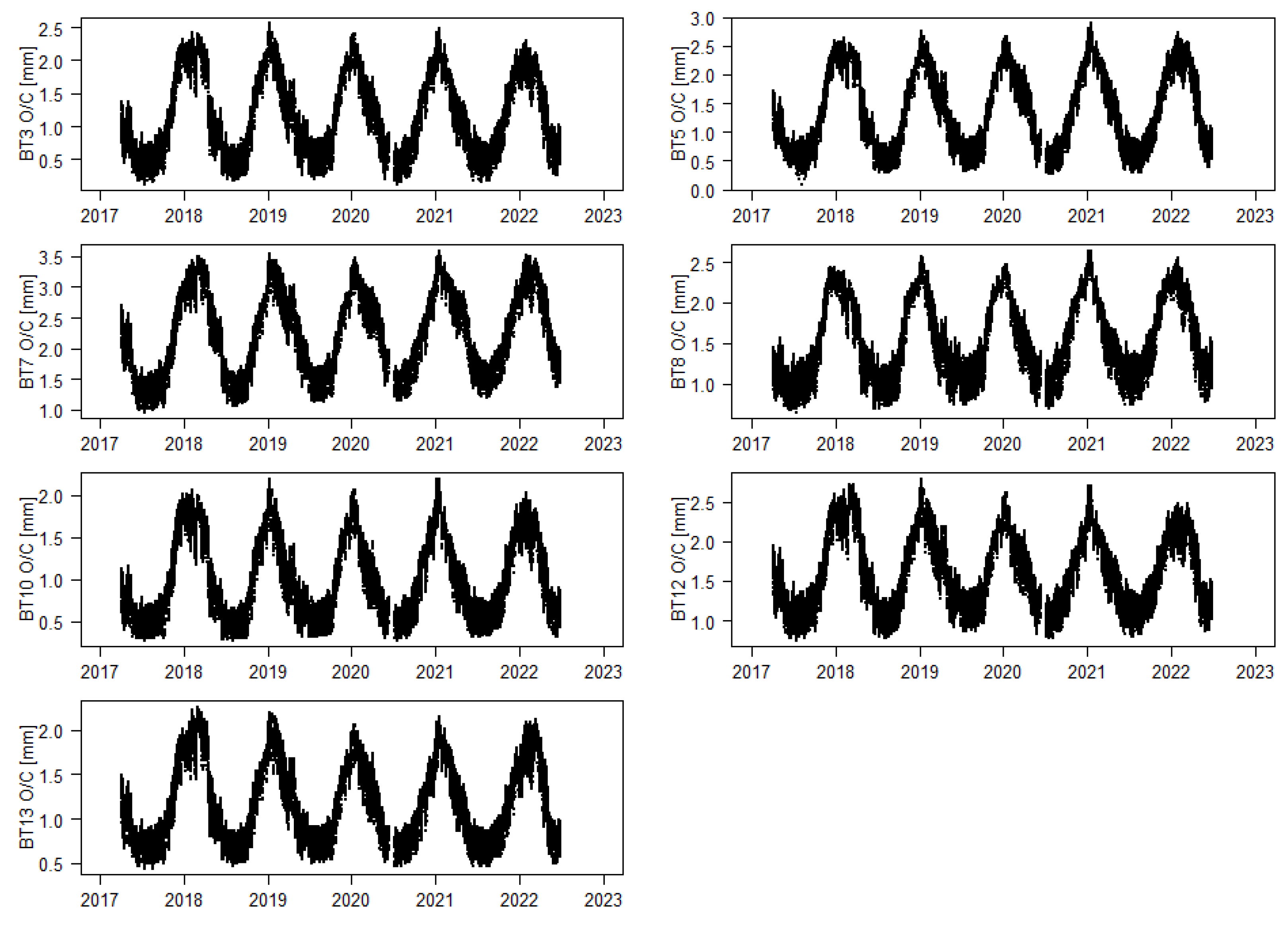
In this case study, the daily variation of the opening-closing movements between blocks measured at the 134.2 m level and through 3D jointmeters were analysed (jointmeter designed by BT3, BT5, BT7, BT8, BT10, BT12, and BT13).

The location of the jointmeter part of the automated monitoring system is shown in Figure 6. The data analysed correspond to a period between April 2017 and June 2022, with more than 38,660 records per variable. Measurements from the automated monitoring system are taken every hour. In the case of gaps in records, the values were estimated by interpolation between consecutive records. The manual and the automated measurements of the opening-closing movements were compared, showing the good performance of the two measurement systems (this comparison is not part of this study).

The samples regarding the relative movements between blocks were collected every two weeks for manual measurements and every hour for automated measurements, as seen in Figure 7. Signs (+) indicate opening movements, and signs (−) indicate closing movements.

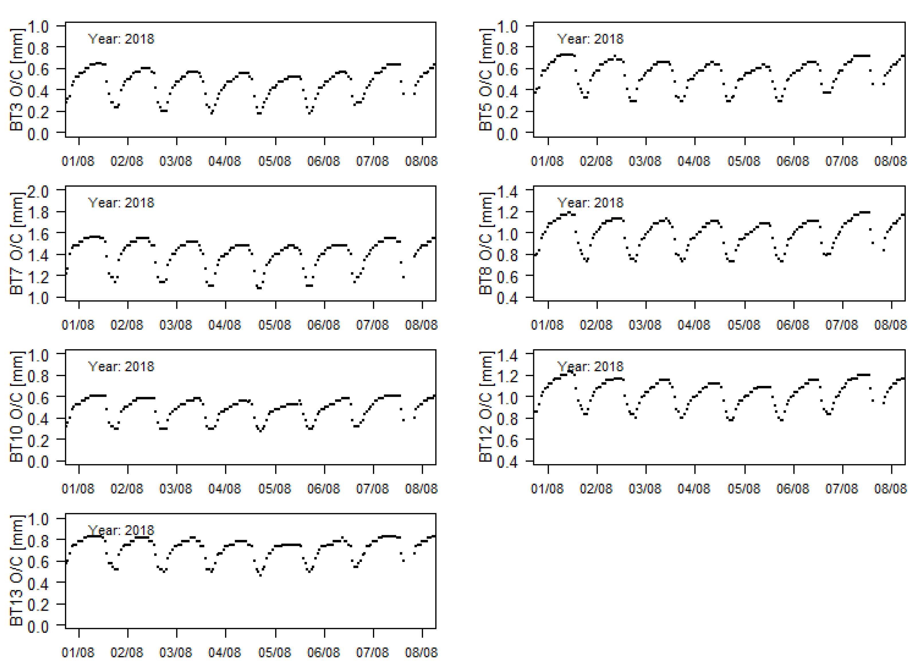
Once the measuring devices to be studied in this work were installed in the downstream face of the dam body (a visiting gallery at the level of 134 m is nonexistent), they measured the relative movements between blocks in a zone that is strongly influenced by the daily variations of the temperatures, as shown in Figure 8, regarding the measurements between the 1st and the 8th of August 2018.

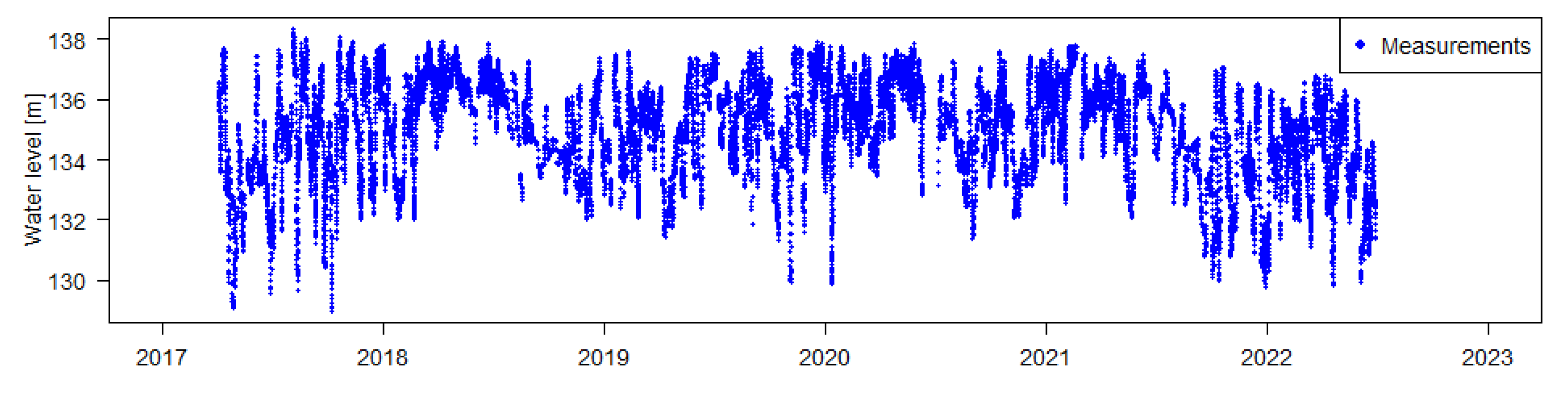
Among the different loads acting on concrete dams, it is typical to distinguish, as the most important loads for structures in normal operations, the hydrostatic pressure and the temperature variation. The time evolution of the reservoir water level is presented in Figure 9.

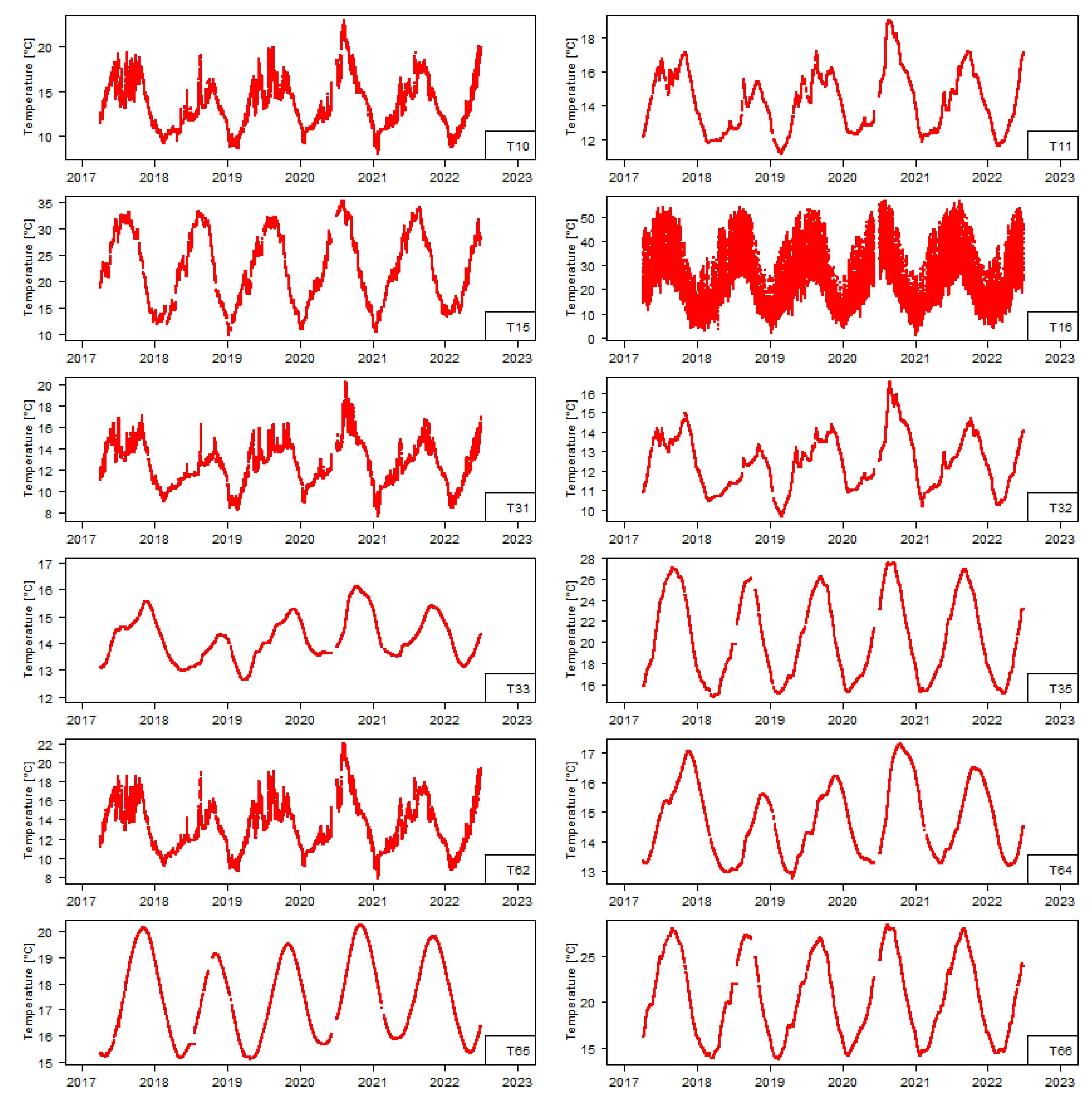
The temperature variations observed in the dam body were recorded through thermometers embedded in the dam body (blocks J7–J8, J11–J12, and J15–J16). The relative position of the thermometers are presented in Figure 6 and

Table 1. Relative location of the thermometers in the dam body.

	Block	Level (m)	Position		Block	Level	Position
T10	J7–J8	122.1	u.f.	T11	J7–J8	122.1	1 m u.f.
T15	J7–J8	122.1	1 m d.f.	T16	J7–J8	122.1	d.f.
T31	J11–J12	112.0	u.f.	T32	J11–J12	112.0	1 m u.f.
T33	J11–J12	112.0	oth	T35	J11–J12	112.0	oth
T62	J15–J16	122.1	u.f.	T64	J15–J16	122.2	oth
T65	J15–J16	122.1	1/2 th.	T66	J15–J16	122.2	oth

Notes: u.f.—upstream face, d.f.—downstream face, oth—other, th—thickness.

, and their records are those shown in Figure 10.

The observations presented in Figure 7, Figure 8, Figure 9 and Figure 10 will be used for the computation of the models presented in this work.

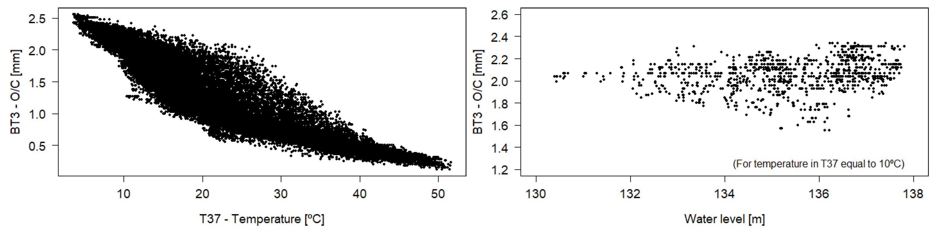
Based on the evolution of the time series of the joint movements, water level, and temperature variations, it is expected that the thermal effect is more significant when compared with the water level effect. Figure 11 presents an example of the temperature and the water height in the structural response for the case study. Figure 11 (left) shows the evolution of opening-closing movement measures in the jointmeter BT3 vs. the temperature measures in the thermometer T37. As expected, the movement between the blocks is in the closing direction when the temperature increases. Figure 11 (right) shows the evolution of the opening-closing movement measures in the jointmeter BT3 and the water height when the temperature measured in the thermometer T37 is 10 °C. The opening movement increases slightly with an increase in the water height.

4. Results and Discussion

4.1. Model Formulation, Construction, and Performance

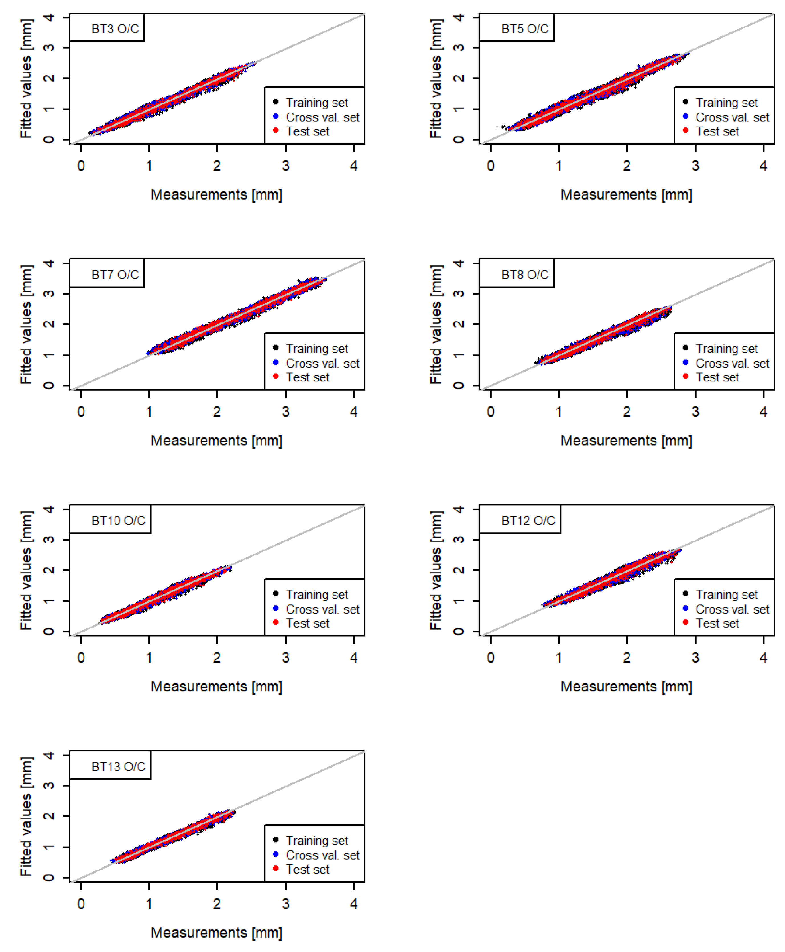
The MLP-NN model based on an HTT approach considered, as an input layer, 15 parameters (representing the hydrostatic pressure—h, $h^2$, $h^4$, where h is the reservoir water level that can vary between 0 and 45 m—and the temperature effects measured at T10, T11, T15, T16, T31, T32, T33, T35, T62, T64, T65 and T66), seven responses at the output layer (representing the opening-closing movements between blocks measured at BT3, BT5, BT7, BT8, BT10, BT12 and BT13), and one hidden layer. Every neuron in the network is fully connected.

A hyperbolic tangent transfer function was chosen as the activation function for the hidden layer, and a linear activation function was chosen for the output layer. The generalized backpropagation delta learning rule algorithm was used in the training process. To find the optimum result (through the minimization of a cost function defined by the mean squared error), 5 initializations of random weights and a maximum of 1500 iterations were performed for each MLP-NN architecture.

A randomization of the learning set was previously carried out, making it possible to define the training set, the cross-validation set and the test set, with a number of examples equal to 65%, 15%, and 20%, respectively. The cross-validation was used as the stopping criteria. In each iteration, the performance for the training set is usually better than before, but if at any time the error for the cross-validation set increases, the NN model may lose its generalization capacity. 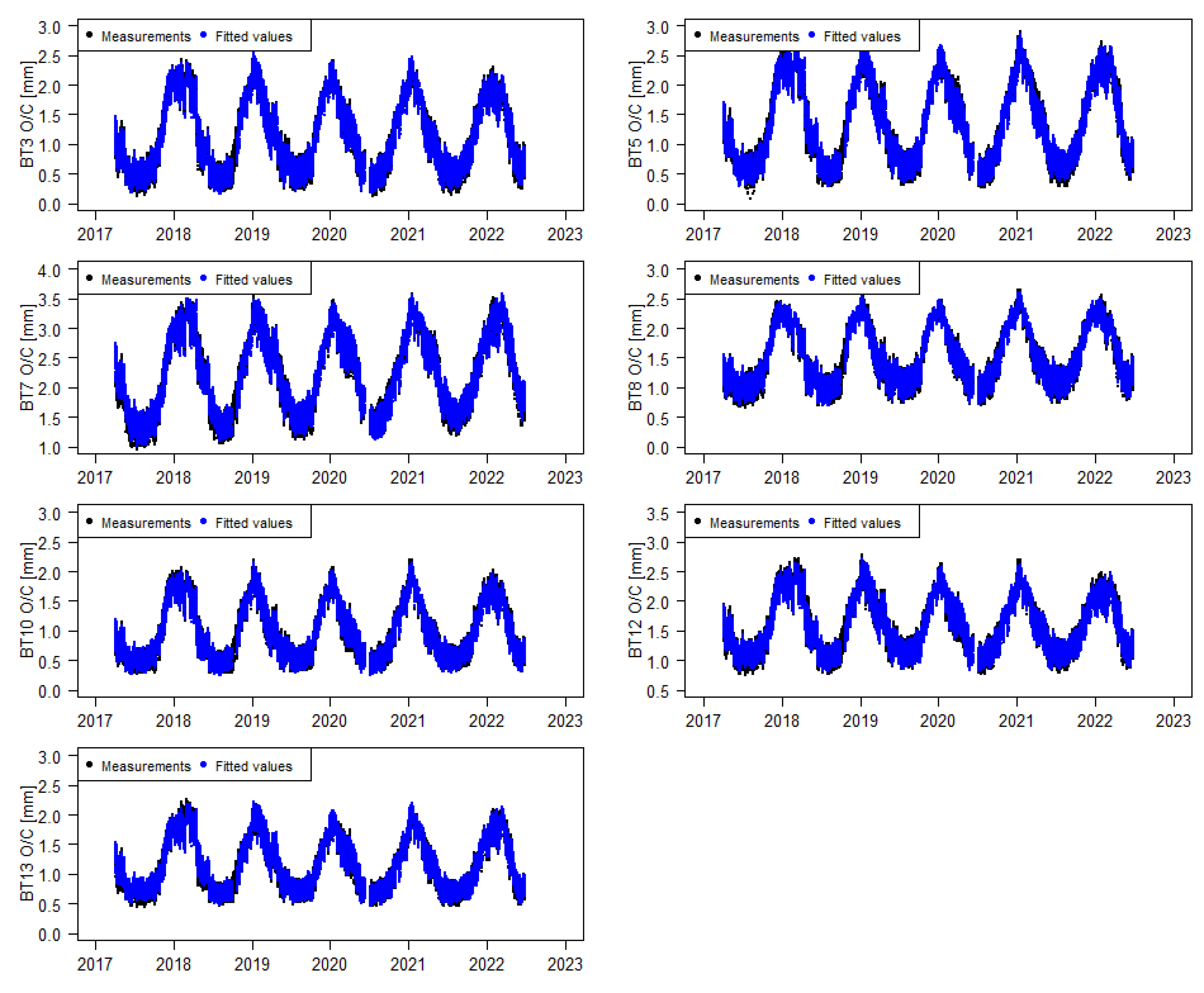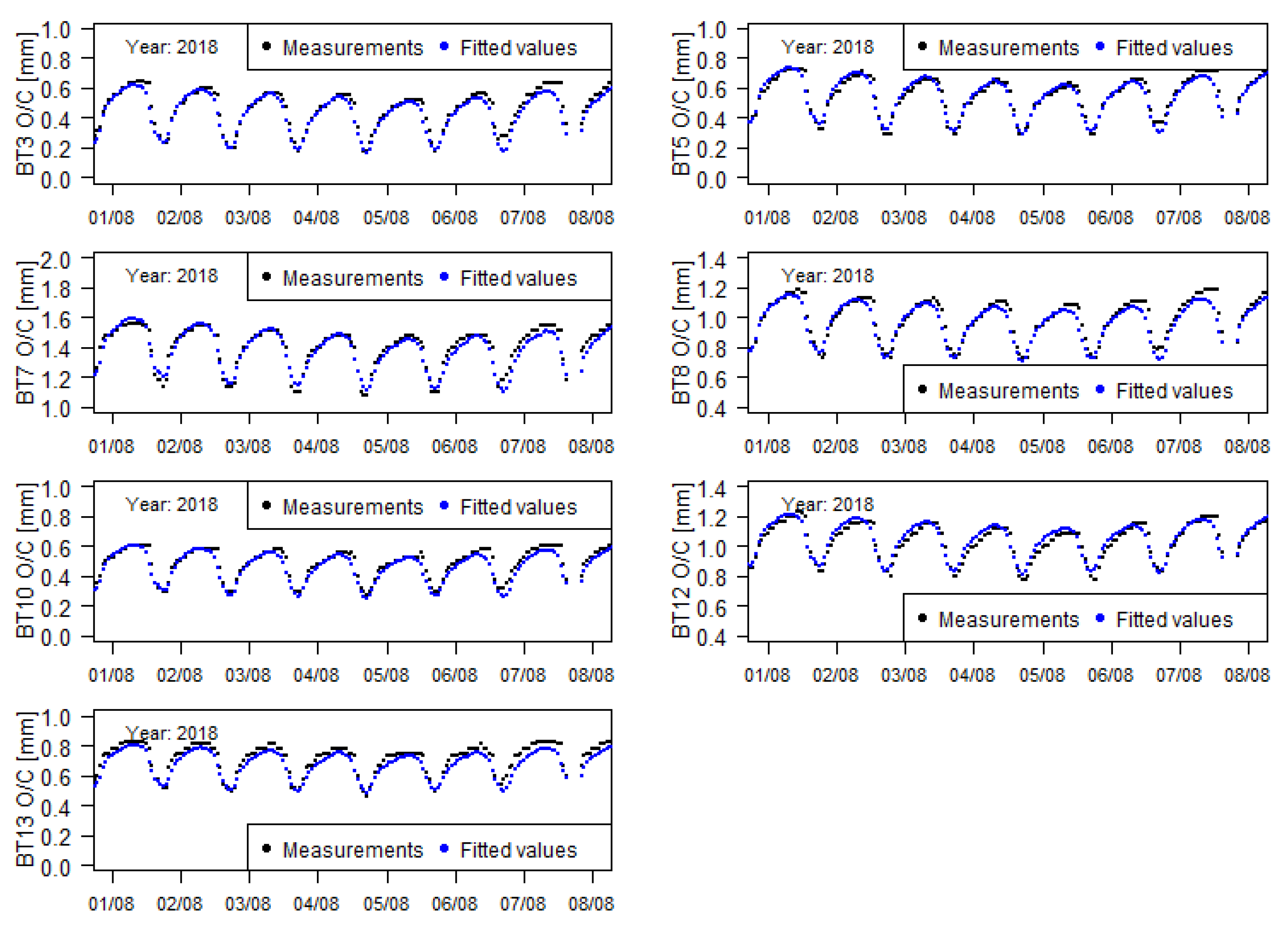The training stops when the error for the cross-validation set begins to increase, with a better generalization thus being ensured [5]. The test set was used as an auxiliary element that enabled us to carry out the quality evaluation of the MLP-NN model for the training set. In this case study, the network with the best performance was a 15-25-7 MLP-NN (less error for the cross-validation set). The results are represented in Figure 12, Figure 13 and Figure 14 and described in

Table 2. MLP model performance parameters.

	Measurements		Model
	Min	Max	rMin	rMax	sd	${\mathit{R}}^2$
	[mm]	[mm]	[mm]	[mm]	[mm]	%
BT3 O/C	0.16	2.56	−0.22	0.35	0.060	99.81
BT5 O/C	0.29	2.85	−0.32	0.39	0.072	99.79
BT7 O/C	1.03	3.57	−0.29	0.33	0.068	99.92
BT8 O/C	0.70	2.61	−0.21	0.34	0.063	99.86
BT10 O/C	0.25	2.15	−0.21	0.30	0.056	99.77
BT12 O/C	0.81	2.72	−0.24	0.37	0.067	99.85
BT13 O/C	0.48	2.21	−0.22	0.28	0.048	99.86

Notes: r—residual, sd—standard deviation, R²—coefficient of determination.

.

4.2. Threshold Definition for a Singular Record

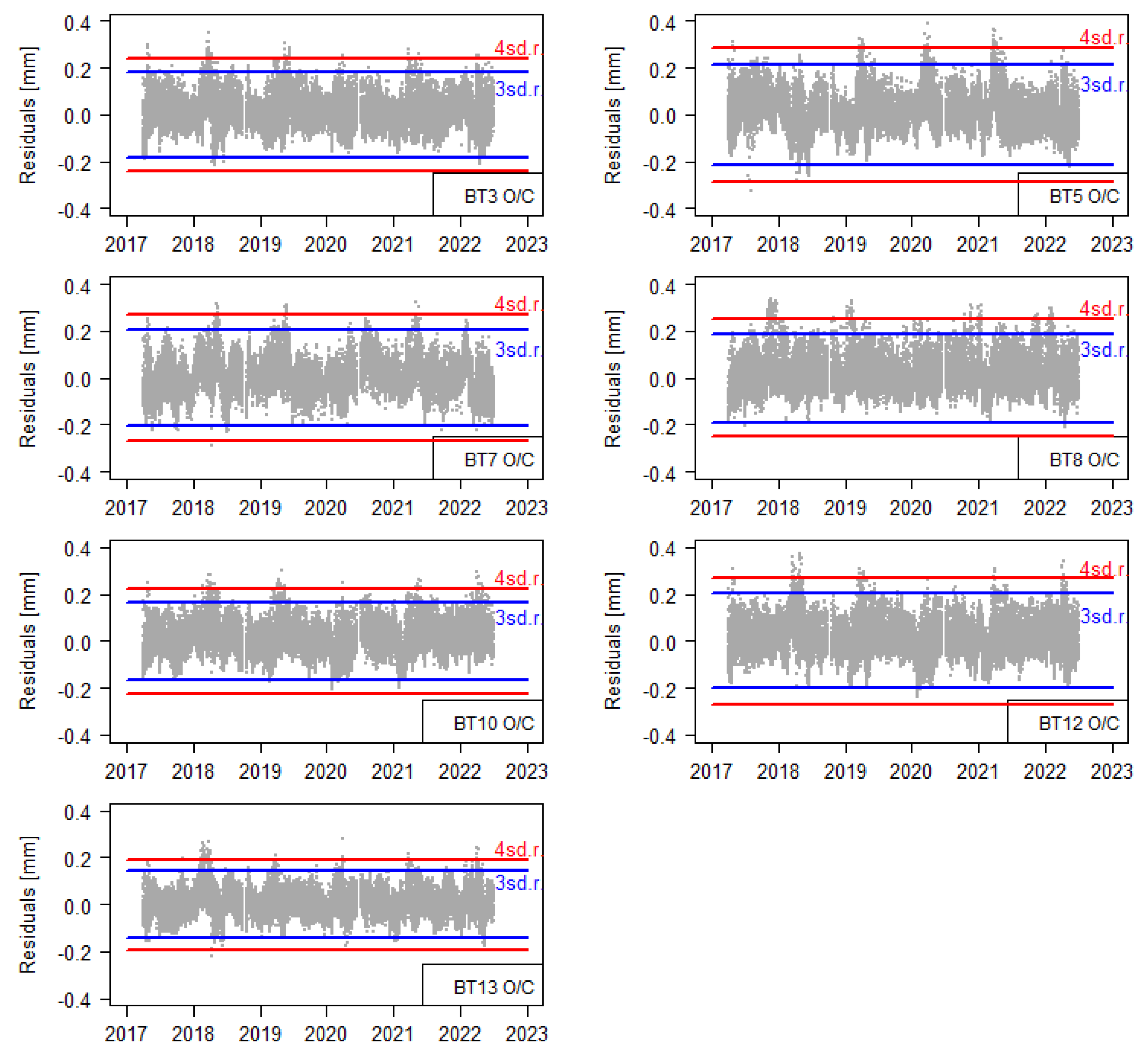
The traditional approach adopted for threshold definition in regression models consists of adopting a multiplicative factor associated with the standard deviation of the residuals. Usually, multiplicative factors equal to 3 or 4, corresponding to a confidence level of 99.73% and 99.99%, respectively, are adopted. This approach assumes that the residuals follow a normal distribution (an assumption that is often not verified for real cases but that allows a good approximation). The same type of criterion can also be used in the MLR-NN model following the limits shown in Figure 15.

4.3. Threshold Definition for Novelty Identification Based on a Time Period Evolution of the Residuals

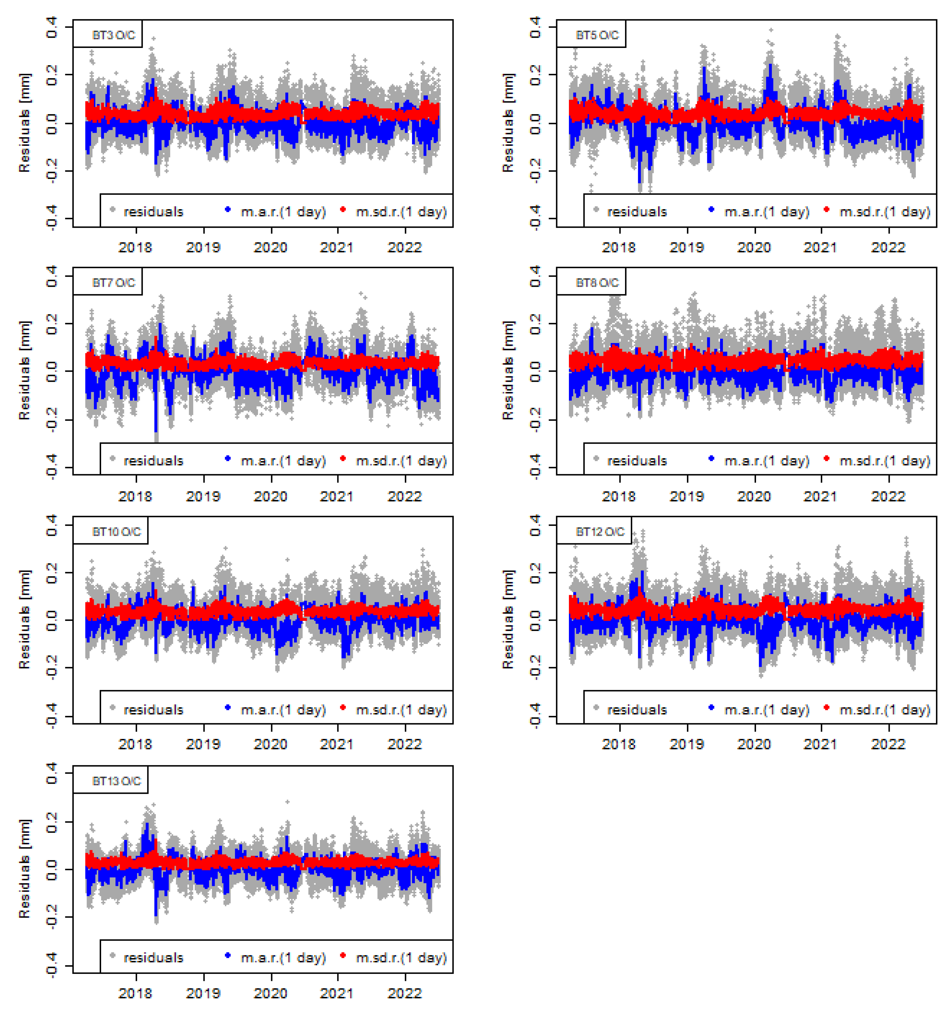
In case a novelty is identified, verifying if it is an isolated record is relevant in order to avoid the false internal warning since, usually, isolated novelties are associated with measurement errors. A critical aspect of dam safety control activities is the pattern recognition in the observed behaviour, including their expected evolution over time. With the exception of extreme load events and other time effects (such as the existence of internal expansion reactions in the concrete), the pattern in the observed behaviour is expected to be continuous over time. Thus, one way to identify novelties in the dam’s behaviour is to analyze the evolution of this behaviour (through the residuals) in a time window along time. Since daily variations resulting from daily temperature changes are observed, a moving window with 24 hourly records and with a time step equal to the measurement frequency (1 h) was adopted.

Figure 16 shows the evolution of the moving average of the residuals ($m.a.r.$) and of the moving standard deviation of the residuals ($m.sd.r.$) in a time window of one day over time.

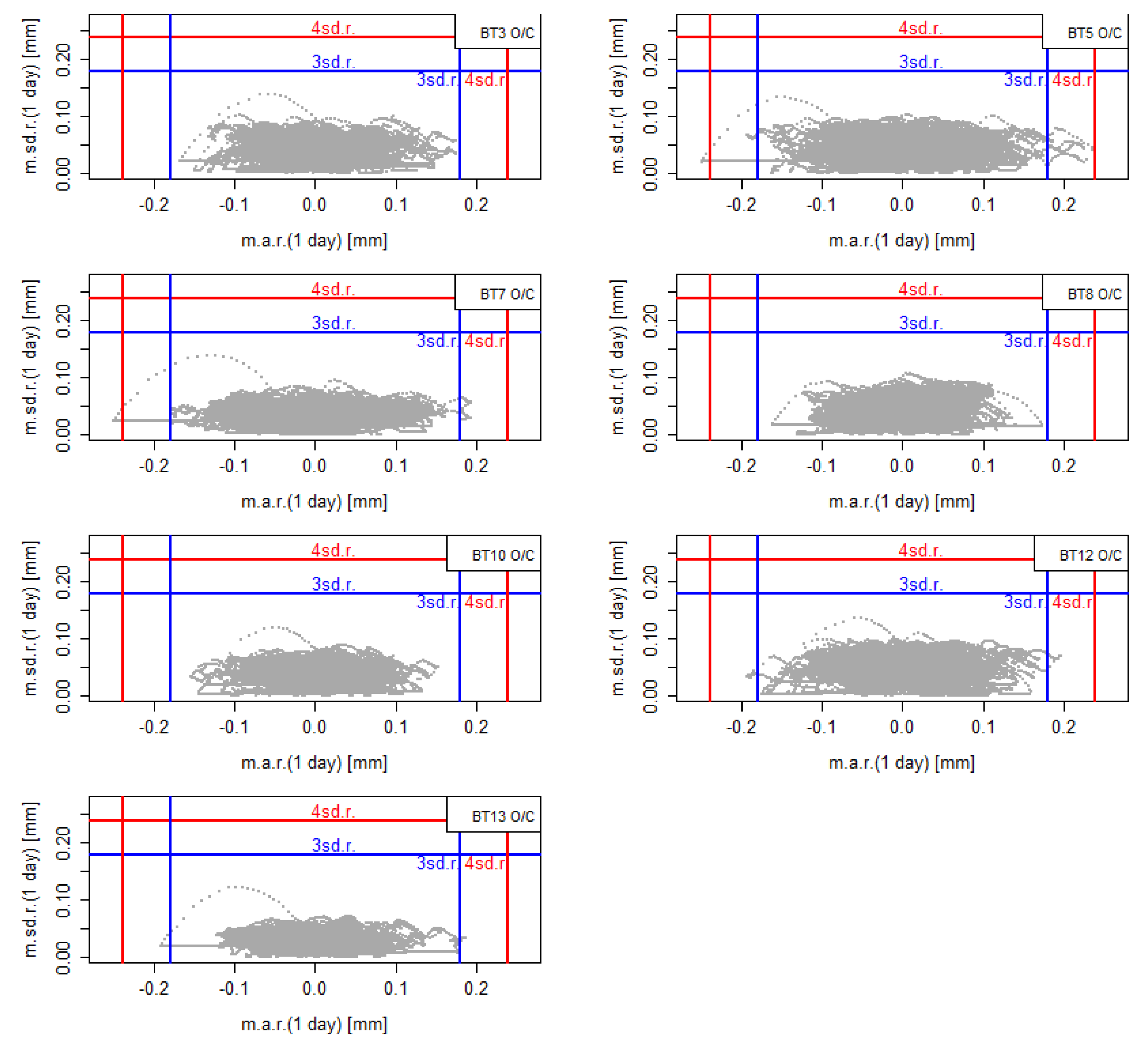
The simultaneous analysis of the $m.a.r.$ and $m.sd.r.$ allows us to identify if the predicted values are moving away from the recorded values (i.e., if the residuals are increasing, meaning that the non-explained part of the model is increasing), and if the residuals increase along time, this could suggest a damage evolution. The definition of thresholds based on multiplicative factors associated with the standard deviation of the residuals is also proposed in this analysis. Similar to the single record analysis, thresholds based on multipliers of 3 and 4 for the standard deviation of the residuals are also proposed, although these values can be updated depending on the results, as seen in Figure 17. The priority in this kind of analysis is to identify periods in which the residuals and their evolution are higher; consequently, a deeper analysis of the data can be carried out.

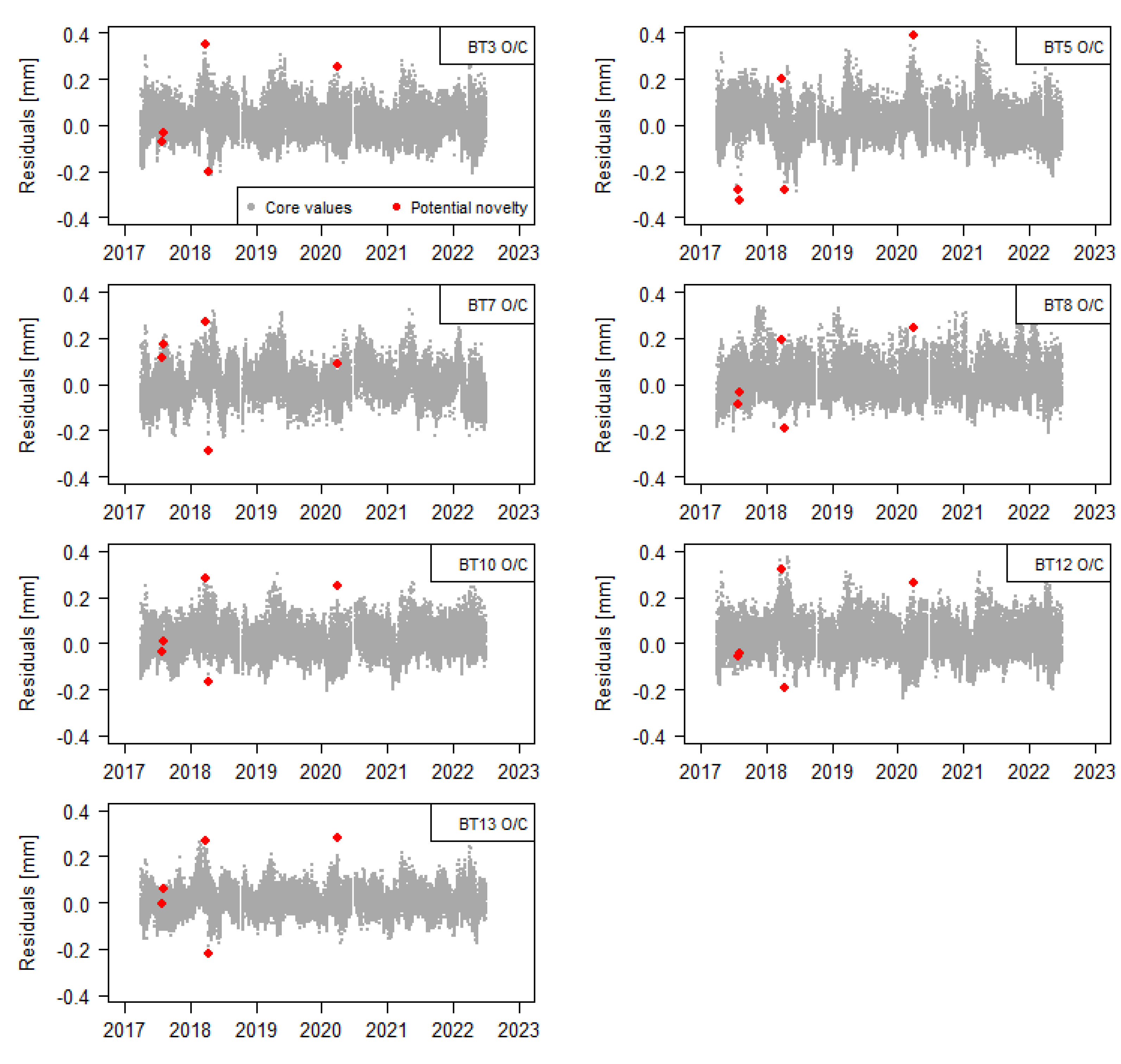
4.4. Threshold Definition for Novelty Identification Based on Multivariate Data

Both of the previous analyses consider one physical quantity at a time. However, considering several quantities at the same time is relevant for an integral judgment. To address this consideration, a threshold definition based on the DBSCAN method is used. By definition, the residuals should follow a distribution similar to a normal distribution with a zero mean. Based on this premise, a criterion for the identification of spread records (in the n features dimension—seven in this case study) that are far from most of the records is defined. An analysis of the effect of the parameters Epsilon and MinPoints were performed as presented in

Table 3. Number of potential novelties based on several Epsilon and MinPoints values.

MinPoints	Epsilon
	0.08	0.10	0.12	0.14	0.16
5	79	9	5	3	0
6	102	12	5	3	1
7	116	14	5	3	1
8	126	22	5	3	1
9	140	22	5	3	1

. Values of Epsilon = 0.12 and MinPoints = 7 were adopted for this case study, as seen in Figure 18. These values were defined based on the specialist criteria considering the standard deviation of the residuals.

The dam behaviour in the time period under study presents a good performance, and there is no abnormal behaviour. The monitoring system records were used for defining the thresholds based on the three proposed procedures. Based on the thresholds defined and for future measurements, the records above the thresholds are the potential candidates to represent a novelty. They should be assessed in order to identify whether they are related to a measurement error or due to other situations.

The analysis of the monitoring data gathered from the horizontal displacements in a concrete dam’s behaviour and the adoption of data-based models to interpret the structural behaviour are common in day-to-day dam surveillance activities.

5. Conclusions and Final Remarks

The analysis of relative movements between blocks through data-based models is unusual due to the nonlinearity of the observed data, which cannot be represented in traditional linear regression models. In this case, a multilayer perceptron neural network (MLP-NN) model was developed to interpret the observed relative movements between blocks. The residuals (the part not explained by the model) resulting from the model were used in this work to define thresholds for novelty identification. The explanatory capacity of the residual analysis allows the definition of a more accurate baseline for the characterization of the structural behaviour. In this work, the analysis of the relative movements between blocks was performed based on hourly recorded measurements. The main inputs considered are the function of the water level and the temperatures measured in several thermometers spread along the dam body. The proposed procedures allow for the earlier detection of novelties through the analysis of the residuals of the MLP-NN prediction model, adopted for the interpretation of the relative movement between blocks, for (i) a singular record, (ii) a moving time period, and (iii) multivariate records. The main issues related to the definition of thresholds can be summarised as follows:

• The definition of univariate thresholds based on the residuals, one for each quantity, is the first recommended step. This approach, through the use of multiplicative factors associated with the standard deviation of the residual, allows an easy novelty identification that, in some cases, could be related to measurement errors.
• The second type of threshold proposed in this study can be defined by the adoption of a moving window with the moving average and the standard deviation of the residuals. This kind of approach allows the specialist to have immediate information concerning the evolution over time.
• Finally, the third type of threshold proposed can be defined based on multiple factors related to the behaviour of the residuals for all the quantities considered in the model. For this approach, a strategy based on the DBSCAN algorithm, which proved to be suitable for multivariate analysis, was used.

To be effective, dam safety control activities must be considered an ongoing process. In this sense, applying the proposed procedures for operational issues in different dams and considering different quantities is suggested. It is important to highlight that each procedure has its singularities and challenges; the observed structural behaviour, the performance of the model adopted, and the quality and frequency of the measurement recorded need to be considered for the adoption of an adequate multiplicative factor for univariate thresholds and the adoption of adequate parameters for multivariate thresholds. The definition of the moving window size for calculating the moving average and the standard deviation depends on the measurement frequency of the records and the reservoir’s exploitation regime. Despite these challenges, the implementation of any of the proposed procedures in an automated monitoring system can adequately support dam surveillance activities.