Article

Water Quality Modelling for Nitrate Nitrogen Control Using HEC-RAS: Case Study of Nakdong River in South Korea

by
Jongchan Kim
1,2,3,*,
Andreja Jonoski
1,
Dimitri P. Solomatine
1,3,4 and
Peter L. M. Goethals
5
1
Department of Hydroinformatics and Socio-Technical Innovation, IHE Delft Institute for Water Education, 2611 AX Delft, The Netherlands
2
K-Water, Daejeon 34350, Republic of Korea
3
Water Resources Section, Delft University of Technology, 2628 CD Delft, The Netherlands
4
Water Problems Institute, Russian Academy of Sciences, Gubkina 3, Moscow 117971, Russia
5
Department of Animal Sciences and Aquatic Ecology, Ghent University, 9000 Ghent, Belgium
*
Author to whom correspondence should be addressed.
Water 2023, 15(2), 247; https://doi.org/10.3390/w15020247
Submission received: 29 November 2022 / Revised: 3 January 2023 / Accepted: 4 January 2023 / Published: 6 January 2023
(This article belongs to the Section Water Quality and Contamination)

Abstract

:
The World Health Organization (WHO) and the U.S. Environmental Protection Agency (EPA) provide guidelines on the maximum levels of nitrate nitrogen (NO3-N) contained in drinking water since excess nitrate ingestion may harm human health. Thus, monitoring and controlling the NO3-N concentration is of paramount importance, especially in sources of drinking water such as the Nakdong River in South Korea. This study addresses NO3-N pollution in the Nakdong River in South Korea, where such pollution mostly comes from diffuse sources in the catchment due to the agricultural use of fertilizers. The objective of this study is to suggest guidelines for designing strategies to control NO3-N in this river using a process-based model developed with HEC-RAS. The model was built based on water quality parameters (water temperature, dissolved oxygen, ammonia nitrogen, etc.) related to NO3-N dynamics incorporating hydraulic and meteorological data. This model simulated NO3-N dynamics downstream under 55 scenarios while focusing on a section near locations of drinking water intakes. The scenarios were constructed based on variations in water quantity and quality upstream. The simulation results showed that the peak concentration of NO3-N downstream could be directly controlled by limiting the NO3-N concentration upstream. Additionally, control of the flow rate upstream could also lead to a reduction in the overall average concentration of NO3-N downstream, but this predominantly occurred when the NO3-N concentration was decreasing. In conclusion, the design and implementation of strategies for the control of NO3-N downstream should be carried out after performing a quantitative analysis of the impact of different control measures for different downstream conditions using a water quality model.

1. Introduction

Climate change has already negatively impacted water resources in terms of quantity and quality [1]. This has prompted increasing interest in ways to effectively improve water quality, especially in rivers and surface water bodies that provide water for the public water supply. A severe reduction in water quality can pose a risk to public health by increasing human exposure to contaminated water [2]. Among the major sources of water pollution, nitrate nitrogen (NO3-N), one of the nitrogen fractions [3], may cause specific cancers and adversely affect human reproduction when people take it in excess [4,5,6]. In this regard, the maximum contaminant level (MCL) of NO3-N has been set to 10 mg L−1 for drinking water by the U.S. Environmental Protection Agency (EPA). The same standard in drinking water has been applied in other countries such as South Korea [7] and Japan [8]. The European Nitrate Directive has required designating areas with surface water or groundwater whose nitrate (NO3) concentration has been more than 50 mg L−1 as Nitrate Vulnerable Zones [9]. The 50 mg L−1 of NO3 or 11.3 mg L−1 (50 mg L−1 multiplied by 0.2258) of NO3-N is identical to the guideline provided by the World Health Organization (WHO) [6]. However, many studies showed that health risks could still be present despite nitrate ingestion below this MCL [6]. Thus, the water quality of reservoirs and rivers needs to be improved by controlling the concentration of this particular pollutant to make it as low as possible since reservoirs and rivers are principal sources of drinking water.
Nitrogen fractions such as NO3-N may flow into reservoirs or rivers due to agricultural practices such as the use of nitrogen fertilizer [6]. Therefore, there is a risk of nitrate contamination in a river catchment with a lot of agricultural activities, such as the Nakdong River in South Korea [10]. Moreover, these pollutants have become water quality parameters that contribute to the complexity of water pollution [11]. NO3-N can be not only risky as a pollutant itself, but some studies indicated NO3-N as one of the main drivers of Harmful Algal Blooms (HABs) [12,13,14]. HABs have caused harm to ecology in an aquatic environment [15] and have threatened public health by producing toxic substances such as microcystin [16,17]. This is especially problematic in South Korea, where HABs have frequently created environmental problems with the four major rivers since 2012, when 16 weirs were constructed resulting in lentic water bodies in the rivers [18,19,20,21]. The specific NO3-N concentration is hardly possible to be indicated in terms of preventing or minimizing HABs because the relationship between NO3-N and HABs depends on other factors such as the state of water flow, site-specificity, and weather. Nevertheless, if the NO3-N concentrations are controlled when flowing into a river or reservoir, a beneficial effect can be achieved for both the aquatic environment and public health.
A water quality model can be an effective and essential tool from the perspective of Water Quality Management (WQM). A well-developed model can help decision makers take proper precautions or emergency actions. Strategies designed with a water quality model would be more cost-effective than others, especially if they involve establishing new infrastructures or imposing government regulations [22] to control water pollution. However, success in WQM based on water quality modelling is dependent on the use of reliable data for the model setup and high performance of the developed model.
Model selection is made with consideration of various conditions including research purposes, data collection, and the required level of model performance [23]. Models (including water quality models) can be generally classified as process-based and data-driven models [24,25]. The process-based model is based on scientific theories or knowledge, while the data-driven model uses data analytics or statistical techniques. Users must select a model that meets optimum conditions after understanding its advantages and disadvantages. To achieve the desired results by developing a process-based model, the user should fully acknowledge the fate and transport of water quality parameters [26,27].
There are various modelling systems that have the capability to simulate NO3-N dynamics in catchments and rivers—for instance, CE-QUAL-W2, SWAT, WASP7, MIKE11 [28,29], and HEC-RAS [30,31,32,33,34,35]. Developing water quality models generally requires many kinds of input variables, which is challenging for model developers [36]. Nonetheless, HEC-RAS outweighs other one-dimensional river water quality models in terms of user interface and ease of model development, although it has not been widely used compared to the others. HEC-RAS allows users to simultaneously develop a hydraulic and a water quality model [32]. In addition, HEC-RAS ensures the reproduction of river flows as realistically as possible when there are inline structures such as a weir in a river. This is because it is well-equipped with various structures for geometric data and numerous boundary condition types [32]. Several studies on water quality have recently been conducted based on these advantages of HEC-RAS. A recent study showed tangible results for nitrogen dynamics linked to unsteady flow [33], while most studies on water quality models developed with HEC-RAS were limited to the analysis of steady flow [30,31,34,35].
We aim to set out the guidelines for designing strategies to control the NO3-N concentration using a process-based model developed with HEC-RAS for the Nakdong River. This river is an important water source for many cities located in the southeastern part of South Korea. Specifically, we first produced a model of NO3-N dynamics for the target area of the upper Nakdong River using HEC-RAS and data from 2019 to 2020. The water quality model was developed based on the hydraulic model of unsteady flow. The downstream boundary of the model was in the vicinity of the Chilgok Weir, which is 135 km away from the upstream boundary. Second, we simulated the change in NO3-N concentration at the location of Chilgok Weir by using the model developed in the first step. For this purpose, 55 scenarios were constructed with variation in water quantity and quality at the upstream boundary. Finally, we generated guidelines for the design of strategies to control the concentration of NO3-N at the Chilgok Weir. These guidelines were based on the scenarios of the second step.
To the best of our knowledge, this is the first study for the Nakdong River designed to use HEC-RAS for the development of a river water quality model linked with unsteady flow. The novelty of this study is based on an in-depth analysis of the change in NO3-N concentration in the lower reach of a river under controlled conditions of the upstream boundary such as water quantity and quality. The methodology presented in this study may also be applied for controlling HABs when linked to research that suggests NO3-N is the main driver of HABs.

2. Materials and Methods
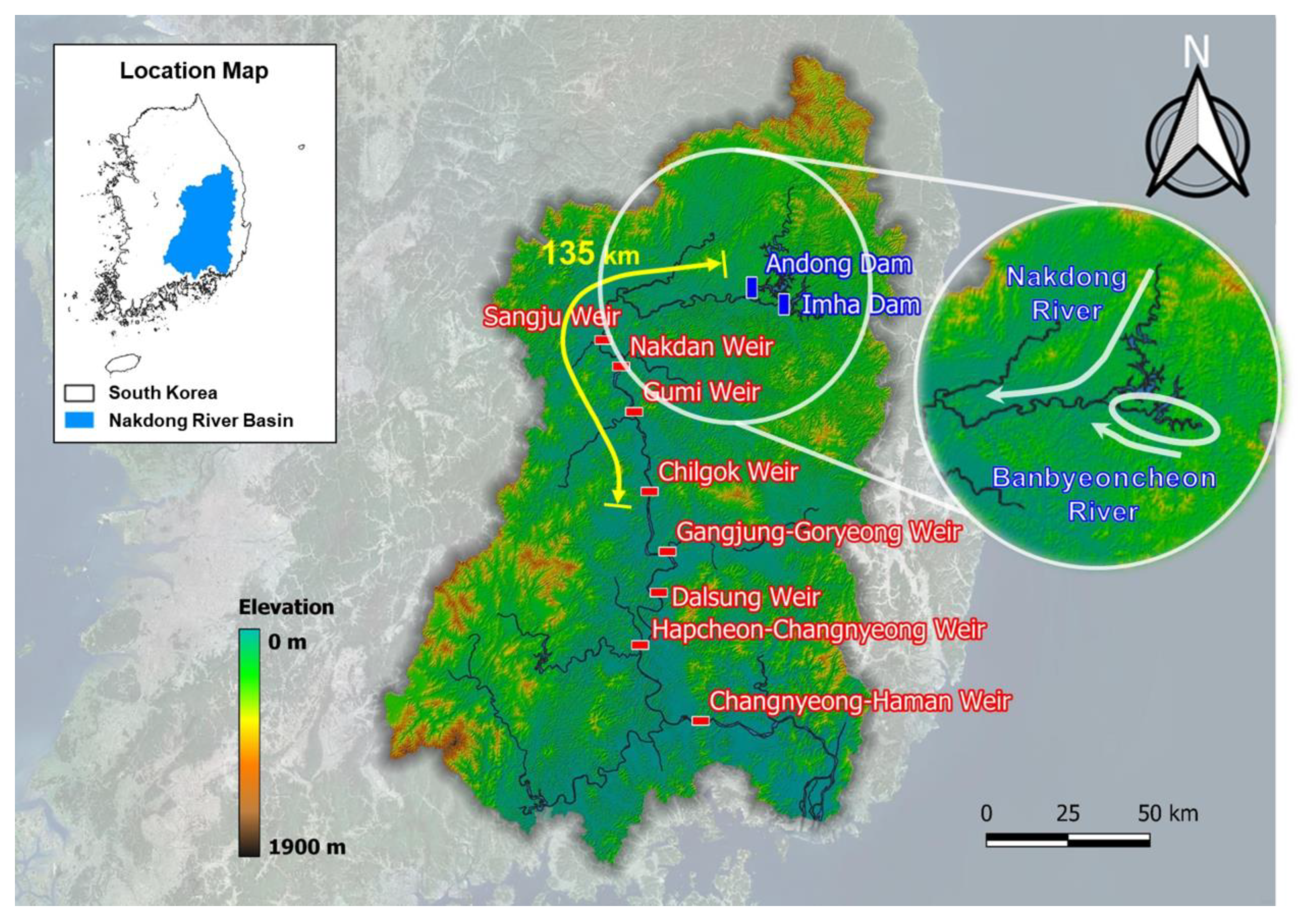
2.1. Study Area

The Nakdong River is the longest in South Korea, with a length of 510 km. The water quality of the Nakdong River has been a matter of concern to environmental authorities since the Nakdong River has been used as a major source for drinking water in adjacent cities [37]. The special importance of WQM in the Nakdong River has arisen from the phenol spill accident that happened in 1991 [38]. Moreover, research studies have dealt with quantitative changes in the water quality of the Nakdong River since 2012, when eight weirs were constructed [37,39,40].
We selected the upper reach of the Nakdong River for this study as shown in Figure 1. The study area covers 135 km in length from the confluence of the Nakdong River and the Banbyeoncheon River to the Chilgok Weir. From 2019 to 2020, the flow rate in this area varied from 5 to 4680 m3 s−1 and the NO3-N concentration varied from 0.240 to 3.099 mg L−1.
The Andong Reservoir and the Imha Reservoir are located most upstream in the Nakdong River and the Banbyeoncheon River, respectively. The Andong Reservoir and the Imha Reservoir are connected by a water transfer tunnel for joint operation in terms of water supply, flood control, and WQM [41,42]. The Imha Dam in particular has a Selective Withdrawal Facility (SWF), so the water quality can be controlled when the water in the reservoir is released downstream [43]. Table 1 shows the details of the Andong and Imha reservoirs [44].
There are four weirs in the study area, including the Sangju Weir, the Nakdan Weir, the Gumi Weir, and the Chilgok Weir. Given that the intake facilities for drinking water are located between two cross sections of the Gumi Weir and the Chilgok Weir [45], the water quality for this district should be managed properly. Table 2 shows the details of four weirs [39,46]. The water level of each weir is usually maintained at each water level specified for management [47] through the operation of the gates.

2.2. Model Description

We used HEC-RAS version 5.0.7 for this study. HEC-RAS has several capabilities such as analysis of steady flow and unsteady flow, simulation of sediment transport, and simulation of fate and transport of water quality parameters [32]. Of these functions, we focused on the module for the river water quality analysis, which was first added to version 4.0 in 2008. The analysis of steady or unsteady flow should precede a water quality analysis [32]. As we had to consider the operations of the four weirs, we performed the analysis of unsteady flow [48] ahead of simulating the dynamics of NO3-N, which is an output variable for this study.
HEC-RAS allows users to build a river water quality model combined with an unsteady flow analysis with inline structures including a weir. This modelling system analyzes unsteady flow by solving the Saint-Venant equation with the implicit finite difference method. The module for analysis of unsteady flow enables the application of several boundary conditions such as stage hydrograph, flow hydrograph, lateral inflow hydrograph, elevation-controlled gates, and so forth [32]. These various boundary conditions help to replicate river flows as realistically as possible. HEC-RAS also solves the one-dimensional Advection–Dispersion equation for water quality analysis using an explicit numerical method called QUICKEST–ULTIMATE (Quadratic Upstream Interpolation for Convective Kinematics with Estimated Streaming Terms–Universal Limiter for Transient Interpolation Modelling of the Advective Transport Equations) [32,49,50]. The module for water quality analysis simulates the fate and transport of water temperature, dissolved oxygen (DO), carbonaceous biochemical oxygen demand (CBOD), and nutrient components such as NO3-N [32].

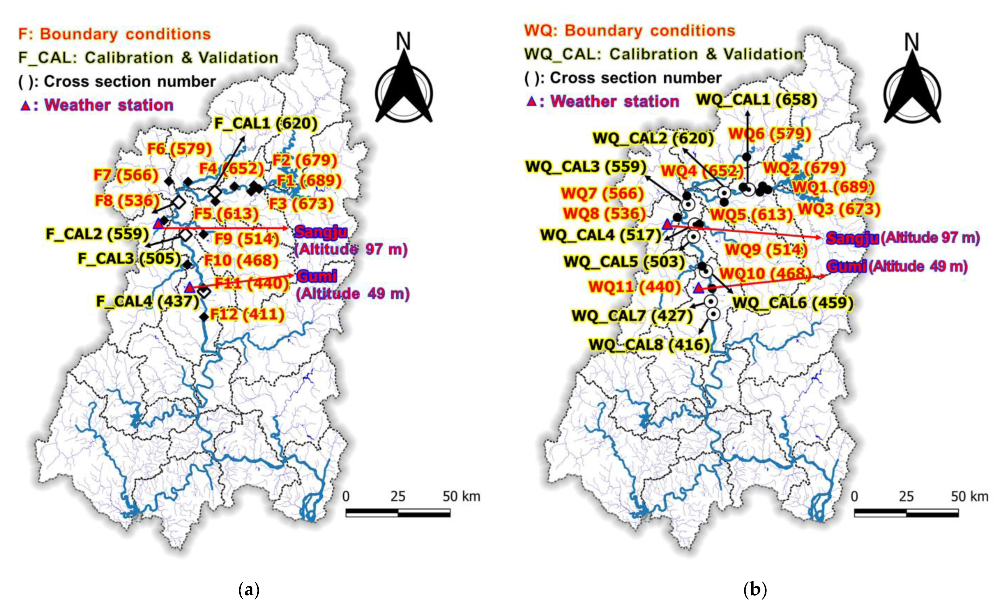
2.3. Data for HEC-RAS Model

2.3.1. Data Availability

HEC-RAS requires geometric data, parameters, hydraulic data, water quality data, and meteorological data for the development of a water quality model [32]. The geometric data include the geometry of cross sections and the inline structures such as a weir [32]. Parameters for a flow model incorporate Manning’s roughness coefficients of each cross section and the status of inline structures (e.g., gate conditions at weirs) [32]. For water quality, parameters include dispersion coefficients and different coefficients controlling the rate of change of different compounds with chemical reactions [32]. Furthermore, HEC-RAS needs hydraulic data such as flow rate, water quality data such as water temperature and concentrations of pollutants, and meteorological data such as atmospheric pressure [32]. When different nutrients are modelled (such as NO3-N), their conversion rates (named ‘pathways’ in HEC-RAS) may be temperature dependent, and water temperature variations are modelled using the meteorological data [32].
The geometric data were obtained from the Basic River Plan for the Nakdong River, including Manning’s roughness coefficients for cross sections (numbered in HEC-RAS as 411–689, see Figure 2) and the inline structures. The River Act of South Korea says that institutions for river management should make a ten-year plan for river management called the Basic River Plan and confirm its validity every five years if necessary [51]. The Basic River Plan for the Nakdong River was made in 2013.
We collected data related to water quantity, water quality, and climate from the Water Resources Management Information System, the Water Environment Information System, and the Open MET Data Portal of South Korea, respectively [52]. The Act on the Investigation, Planning, and Management of Water Resources states that the institutions dedicated to hydrological investigations have to operate information systems to efficiently manage data for water resources [53]. The Ministry of Environment forms a national network to periodically monitor water quality and manages water quality data through an information system under the Water Environment Conservation Act [54]. The Korea Meteorological Administration runs an information system for meteorological data and provides the data to citizens under the Weather Act [55]. All data for the development of the HEC-RAS model are publicly available from the information systems operated under these Acts.
The observational data were retrieved from 16 monitoring stations for hydraulic data, 19 monitoring stations for water quality, and two weather stations (Sangju and Gumi). The location of these stations is shown in Figure 2. The daily data are available for flow rate, water level, and climate, while water quality data is monitored almost weekly (48 or 36 times a year). We collected the data for model development in terms of the fate and transport of NO3-N. The hydraulic data included flow rate and water level. The water quality data contained water temperature, chlorophyll a (Chl-a), dissolved oxygen demand (DO), total dissolved nitrogen (TDN), ammonia nitrogen (NH3-N), and NO3-N. Five types of meteorological data were collected, including atmospheric pressure, air temperature, relative humidity, solar radiation, and wind speed. Table 3 shows the mean, minimum, and maximum values of the observational data of flow rate and NO3-N in the cross sections for model calibration (2019) and validation (2020).

2.3.2. Data Preparation

We preprocessed some raw data to make them suitable for model development. The reason we needed this process is that the observational data and their frequencies do not exactly correspond to those required in the modelling system. HEC-RAS requires water temperature, algae, DO, carbonaceous biochemical oxygen demand (CBOD), dissolved organic nitrogen (DON), ammonium nitrogen (NH4-N), nitrite nitrogen (NO2-N), and NO3-N [32] as water quality parameters related to NO3-N dynamics. To address the problem of such discrepancies between the data, we interpolated the weekly data to convert them into daily data and estimated the data which are not measured—for example, algae, CBOD, and a few nitrogen components.
The following are four processes we went through for data preparation. First, the weekly data for water quality were interpolated so that they were transformed into daily data, which is the same interval as the water level and flow data. We interpolated the water quality data by applying a step function to avoid distortion of the data variation [56]. In other words, the same values as the previous observational data were placed at daily intervals until the next data were available [57,58].
Second, we estimated the algal biomass required as input data by using the observational data of Chl-a, which is often used as a proxy index for HABs [59,60,61]. The concentration of Chl-a can be converted into the algal biomass with the stoichiometric ratio according to Equation (1) [33,61].
100.0 g Algae:40.0 g C:7.2 g N:1.0 g P:(0.4–1.0) g Chl-a
where C is carbon, N is nitrogen, and P is phosphorus.
Third, a few nitrogen fractions such as NO2-N, NH4-N, and DON had to be estimated because they were not monitored [33]. NO2-N was assumed to be zero since it hardly exists in rivers [62,63,64,65]. The concentrations of NH3-N were determined by laboratory experiments using an ion analyzer [18] after converting ammonium ions (NH4+) into ammonia (NH3) by increasing the pH of samples with sodium hydroxide (NaOH). Because NH4+ and NH3 are pH-dependent, NH3-N exists in the form of NH4-N in most aquatic environments [66,67]. We thus replaced the data of NH4-N required in HEC-RAS with the available data of NH3-N. The DON concentration was calculated by subtracting the sum of NH3-N and NO3-N from TDN [3,63].
Lastly, we did not consider CBOD as an input variable because the module for water quality analysis in HEC-RAS calculates only losses due to oxidation and settling for CBOD [32]. We performed the sensitivity analysis on the assumption that the changes in the CBOD concentration at all the boundary conditions would not cause fluctuation in the downstream NO3-N concentration. As a result, the assumption was valid as shown in Figure 3.

2.4. Experimental Setup

To build a water quality model using HEC-RAS, we needed not only the geometric data but also the boundary conditions for modules for both unsteady flow and water quality [32]. We collected the geometric data by extracting the upper reach including cross sections (number 411–689) corresponding to approximately 135 km from the Basic River Plan for the Nakdong River. The daily data of flow rate were entered as boundary conditions for the cross section most upstream in addition to 10 cross sections with lateral inflows. The data of stage hydrograph was provided as a boundary condition most downstream. Regarding the four weirs included in the geometric data, we entered the data of the water levels for management as the boundary conditions of the type of elevation-controlled gate. The boundary condition of the elevation-controlled gate enables the control of the gates of the weirs in time [32]. This control of the gates was automatically taken into account in HEC-RAS based on each water level for the management (see Table 2) of the four weirs. As the boundary conditions for the water quality module, we entered the daily data interpolated from the weekly data in the cross sections where the boundary conditions for flow analysis were already given [32].
We calibrated the model parameters with data from 2019 and validated the model with data from 2020. Since the peak flow in 2019 was larger than in 2020 at the monitoring station most downstream for calibration and validation, the data from 2019 were used for calibration. The warm-up period is also necessary for model development until dynamic stability is achieved for the initial conditions [68]. Therefore, we entered the data for the warm-up period from August to December of the previous years.
The data for unsteady flow were derived from four monitoring stations for calibration and validation. For water quality analysis, we used the data from eight monitoring stations, which is twice as many stations as used for the flow analysis. The reason we used data from more stations for water quality analysis is that figuring out the fate and transport of NO3-N is more important and complicated than flow analysis in this study. These stations were designated in consideration of the locations of the tributaries and the weirs, as shown in Figure 2, which illustrates the location of the monitoring stations. The main parameters related to NO3-N dynamics are the conversion rates, shown in Table 4 [32], and model calibration was performed based on the default values provided in HEC-RAS. Finally, for the dispersion coefficient, we used the HEC-RAS option of automatic computation based on flow data.
We constructed 55 scenarios to understand how the concentration of NO3-N downstream is changed by the variation in water quantity and quality at the upstream boundary. Three components such as flow rate, water temperature, and NO3-N were related to these scenarios. Table 5 shows how we constructed the scenarios using these components. For example, the seventh scenario (Scenario 7) is that the flow rate of the upstream boundary increases by 50 m3 s−1 for 10 days from 1 January.
These scenarios were constructed under the assumption that the water quantity and quality at the upstream boundary can be controlled. In practice, controls on the water quantity and quality can be imposed by the joint operation of the Andong and Imha reservoirs and the use of SWF installed in the Imha Dam [41,42,43]. The maximum increment of flow rate, 150 m3 s−1, was given based on the maximum amount of water that can be released downstream via the generators of the Andong Dam and the Imha Dam. The simulations under the scenarios were carried out with data from 2018 and the developed model.

3. Results

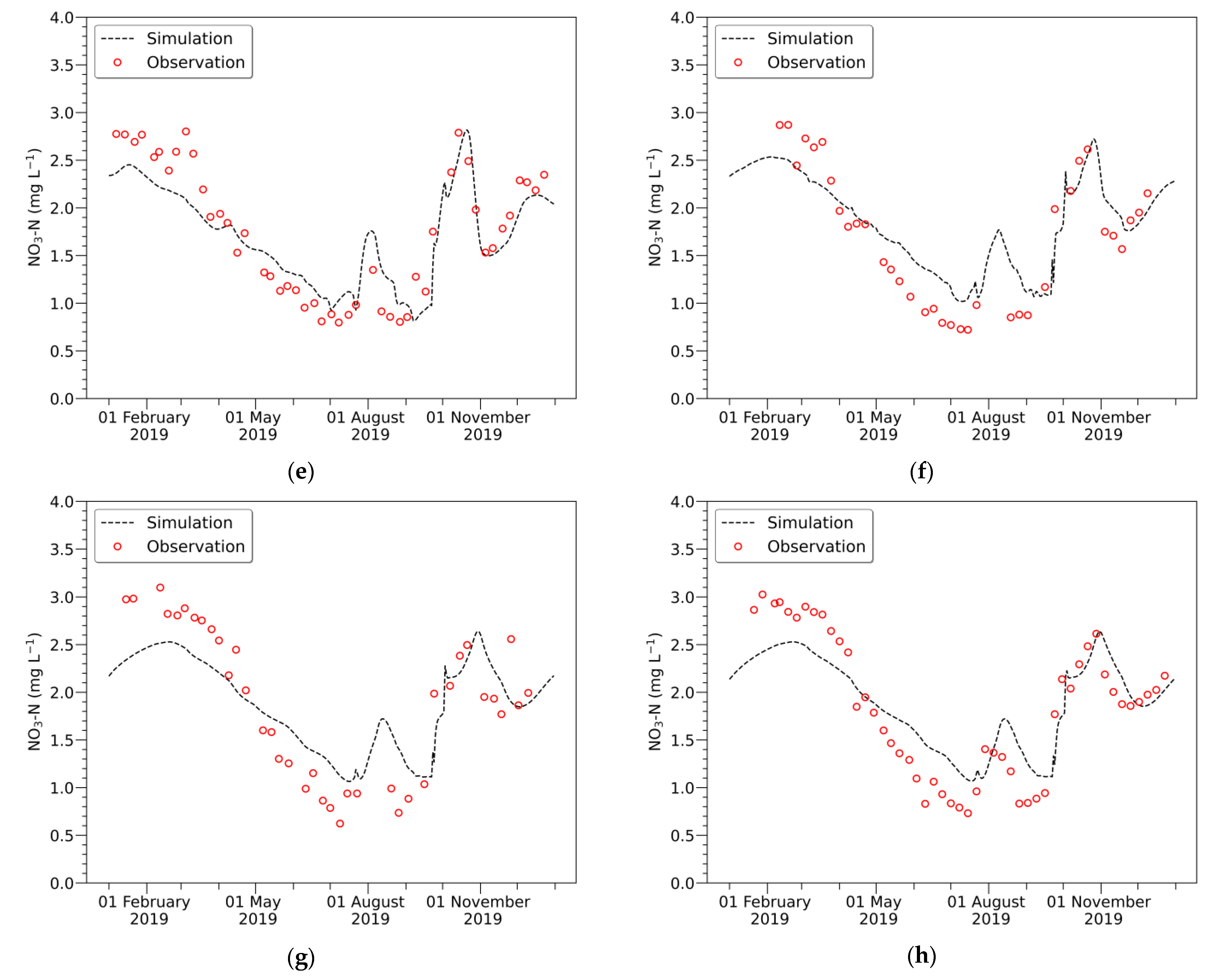
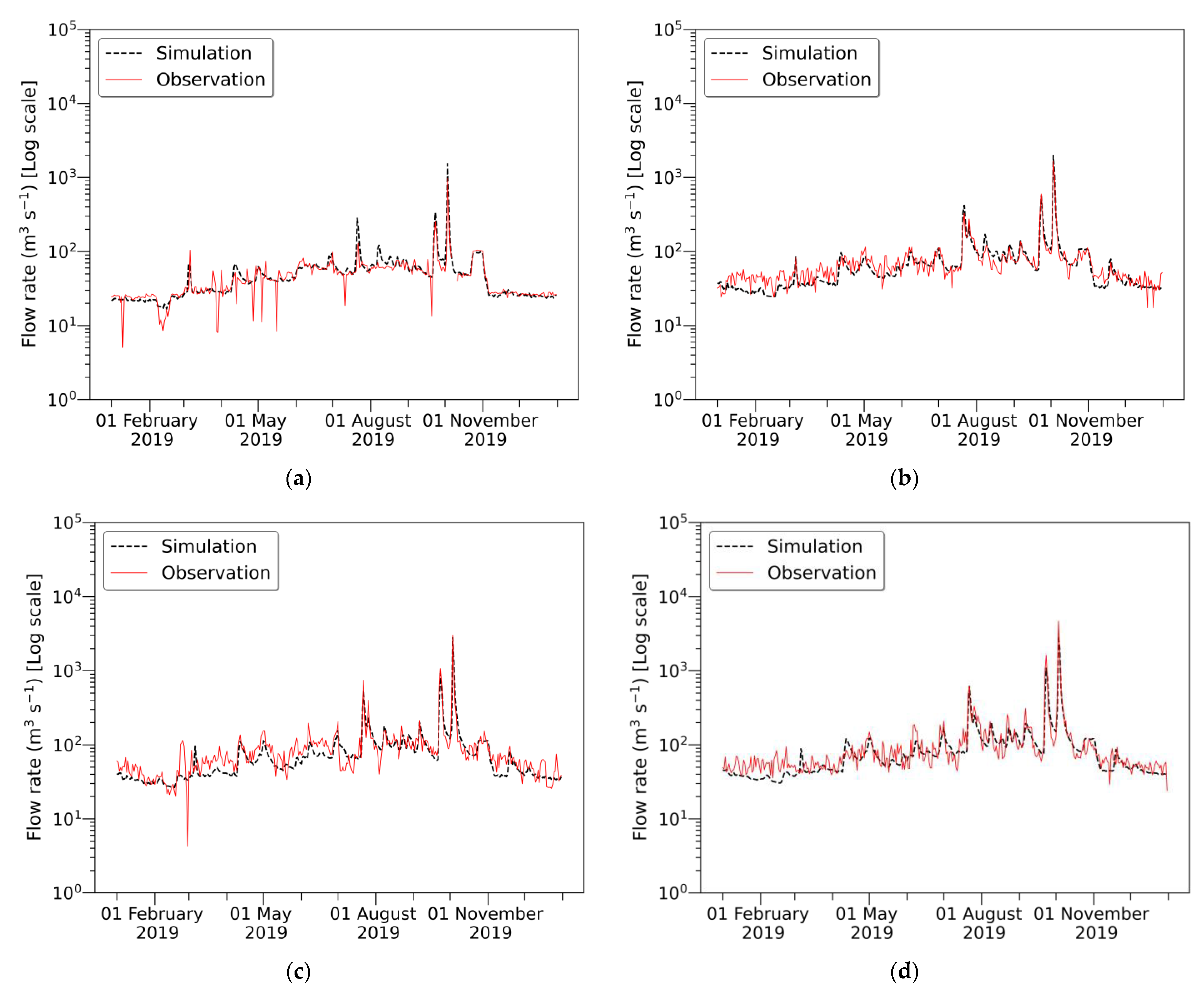
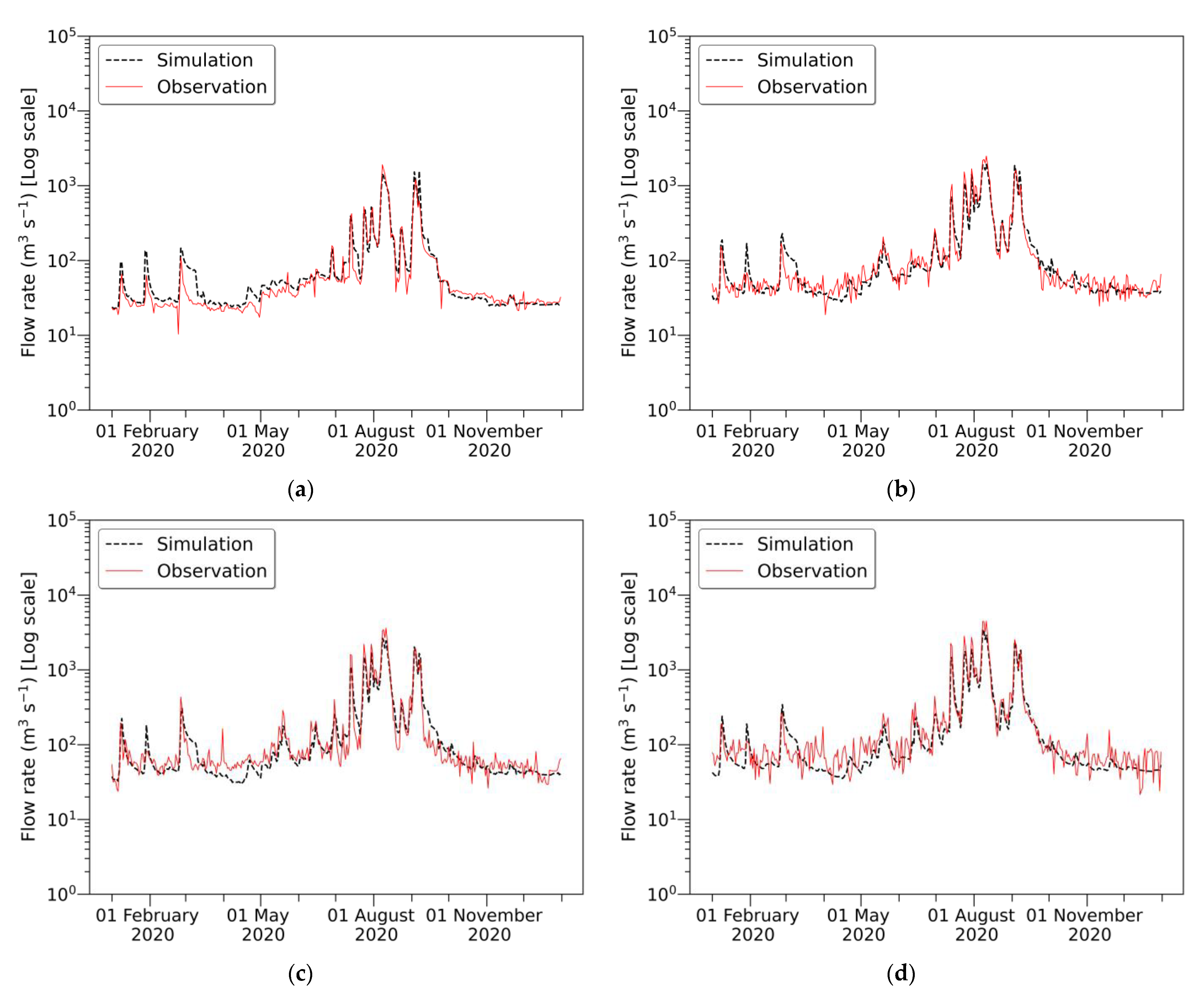
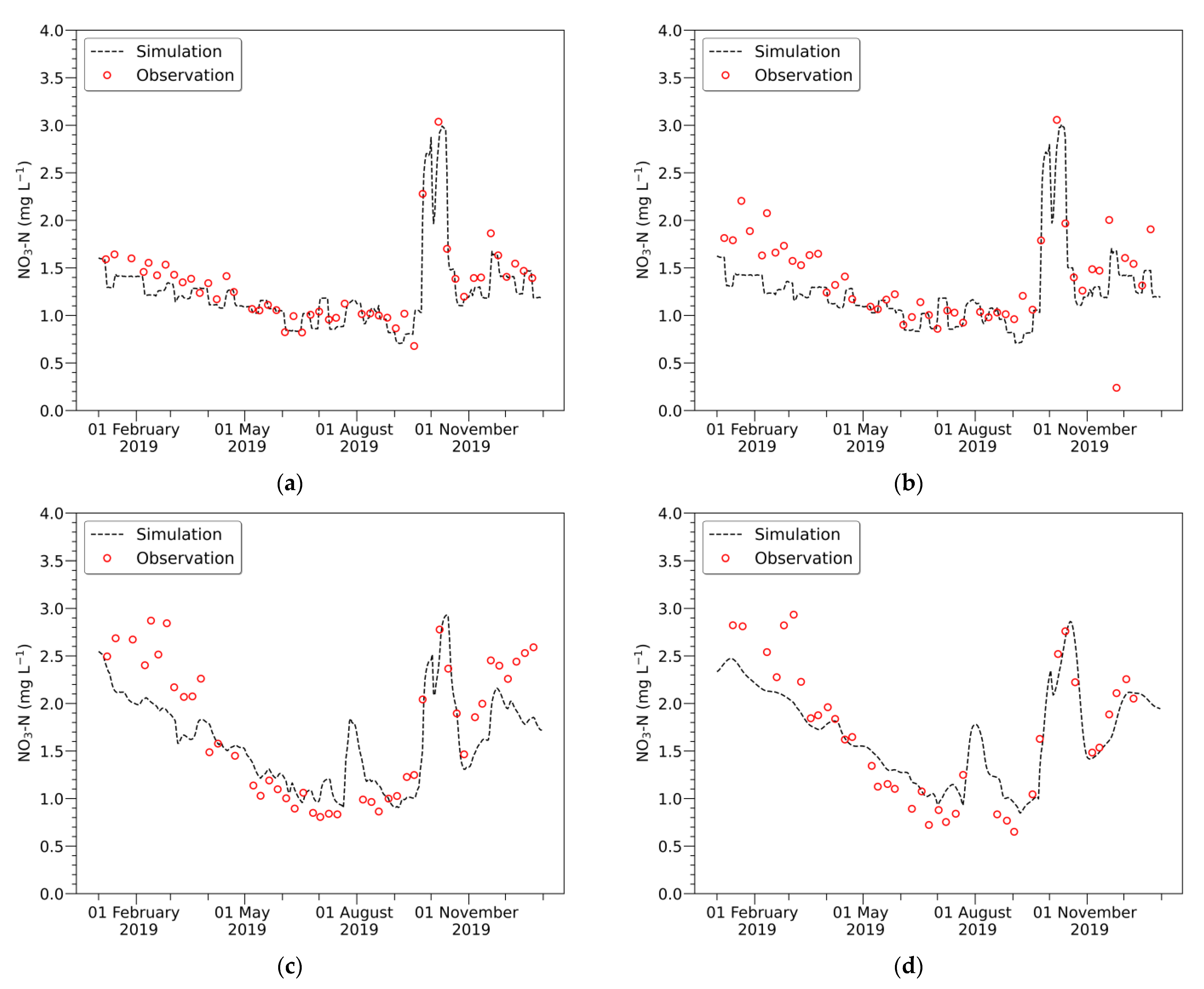
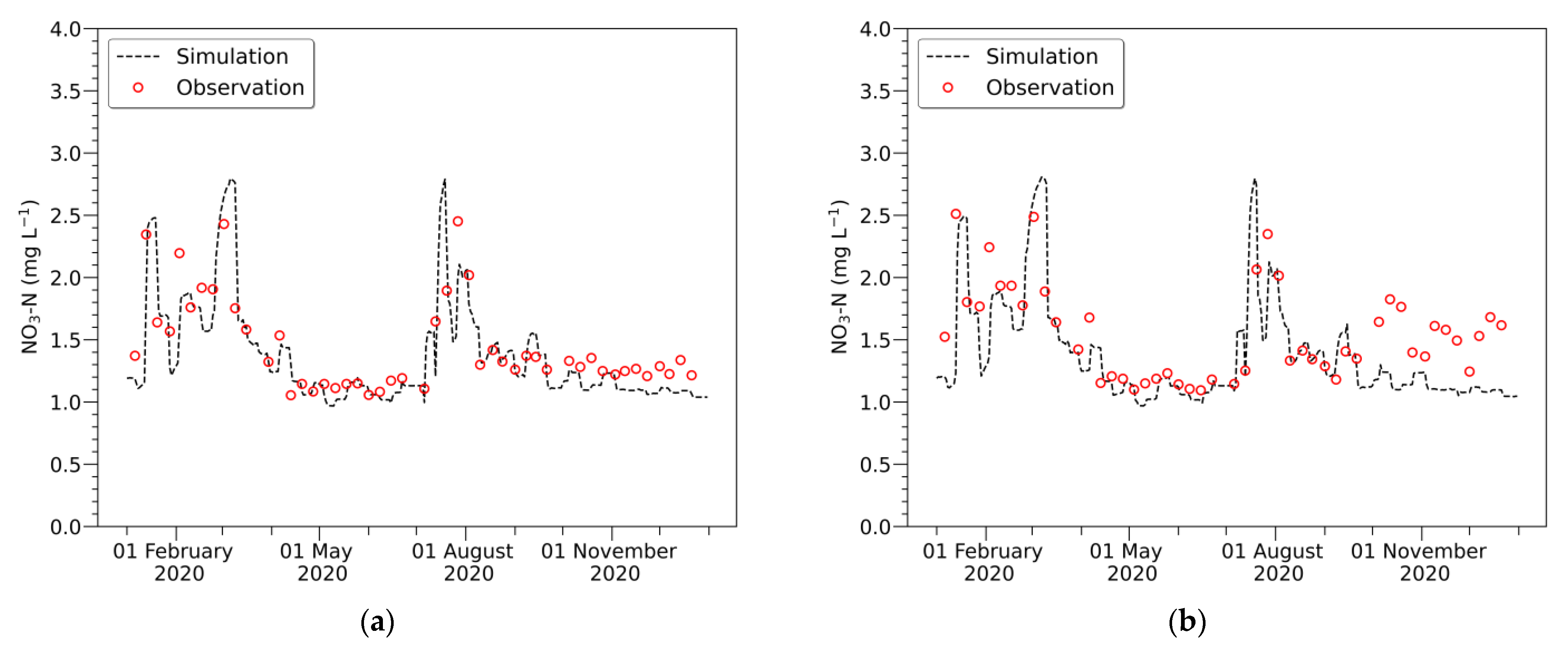
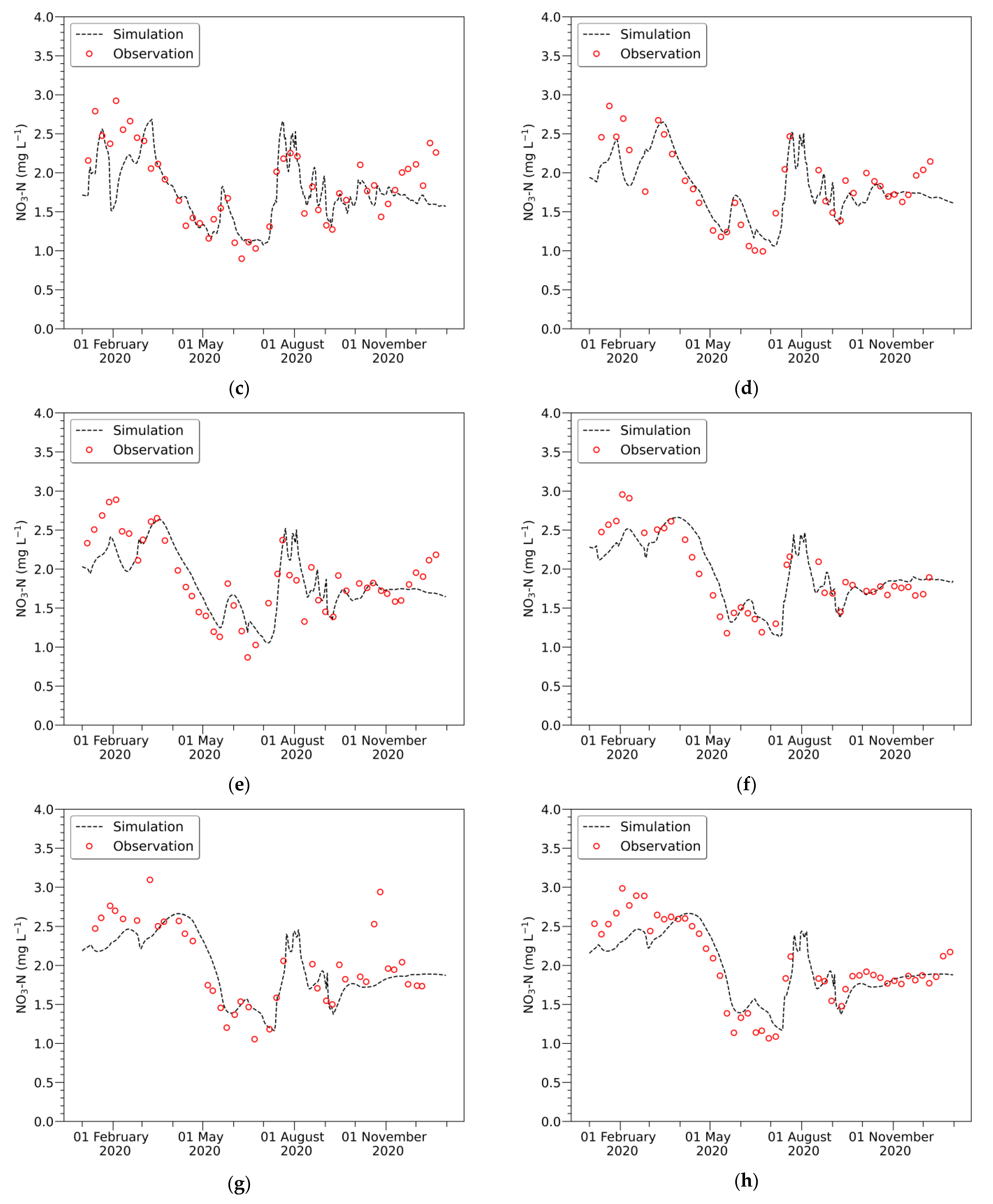
3.1. Calibration and Validation

3.1.1. Unsteady Flow

We used Manning’s roughness coefficients, listed in Table 6, for calibration of the hydraulic model. The Manning’s roughness coefficient is the main parameter for calibration. We obtained the data of the coefficients from the Basic River Plan for the Nakdong River.
Moriasi et al. [69] suggested the criteria of performance evaluation for watershed-scale models using Coefficient of Determination (R2), Nash Sutcliffe Efficiency (NSE), and Percent Bias (PBIAS). According to the study, model performance for flow simulations is “Good” if 0.75 < R2 ≤ 0.85, 0.70 < NSE ≤ 0.80, and ±5% ≤ PBIAS < ±10%, while it is “Satisfactory” if 0.60 < R2 ≤ 0.75, 0.50 < NSE ≤ 0.70, and ±10% ≤ PBIAS < ±15%. These criteria are mainly applied to watershed-scale models, but they can be used for measurement of the performance of our river model built using HEC-RAS. However, we also simultaneously employed a graphical method [69] to assess the quality of the models. Equations (2)–(4) show R2, NSE, and PBIAS, respectively [69].
R 2 = i = 1 n O i O ¯ S i S ¯ i = 1 n O i O ¯ 2 i = 1 n S i S ¯ 2 2
NSE = 1 i = 1 n O i S i 2 i = 1 n O i O ¯ 2
PBIAS = i = 1 n O i S i i = 1 n O i × 100
where O is observational data and S is simulation result.
Unsteady flow was simulated using observational hydraulic data such as flow rate and water level as boundary conditions of HEC-RAS. As a result of both calibration and validation for unsteady flow, we carefully judged that the performance of our model was high overall in consideration of both the quantitative evaluation and the graphical method. The quantitatively measured model performance was more than “Satisfactory” except for one cross section (437), as shown in Table 7. However, the peak flows from the model simulation were not consistent with the observational data according to Figure 4 and Figure 5, so this produced an unsatisfactory outcome of PBIAS in cross section 437. Nonetheless, since the trends in increasing flow were accurately reflected, model performance was judged as high for this unsteady flow model.

3.1.2. NO3-N Dynamics

The water quality model for NO3-N dynamics was developed using the hydraulic model built for unsteady flow. We simulated NO3-N dynamics using the water quality data and the meteorological data as the boundary conditions of HEC-RAS. For calibration and validation, we used the main parameters of the model related to NO3-N dynamics (see Table 4). One model parameter was significantly adjusted during calibration, namely Beta 3, for which a value of 0.001 was applied, while the default values were used for the other model parameters. We simulated the water quality parameters including NO3-N by applying these model parameters. Table 8 shows the mean values of both the observational data and the simulation results for the water quality parameters from 2019 (calibration) to 2020 (validation).
We assessed the model performance for NO3-N dynamics by adopting both the objective criteria established by Moriasi et al. [69] and the graphical method. According to Moriasi et al., model performance for nitrogen (N) is “Good” if 0.60 < R2 ≤ 0.70, 0.50 < NSE ≤ 0.65, and ±15% ≤ PBIAS < ±20%, while it is “Satisfactory” if 0.30 < R2 ≤ 0.60, 0.35 < NSE ≤ 0.50, and ±20% ≤ PBIAS < ±30% at the watershed scale. The gap between the watershed-scale model and our river model was closed by simultaneously employing the graphical method in the same way as when the model performance for flow simulation was assessed.
We judged that we built a robust model for NO3-N dynamics when carefully evaluating model performance at eight monitoring stations. Model performance for NO3-N dynamics was more than “Satisfactory” except for one cross section (620), as shown in Table 9. Figure 6 and Figure 7 show that NO3-N dynamics simulated by the HEC-RAS model had a remarkably similar pattern to the observational data in eight cross sections.
The model delivered high performance, especially in cross section 416, which is closest to the Chilgok Weir. The station in this cross section is located most downstream among the eight monitoring stations for calibration and validation. Cross section 416 is critically important in this study because the scenarios, provided in Table 5, were constructed for the simulation of NO3-N dynamics in cross section 416.

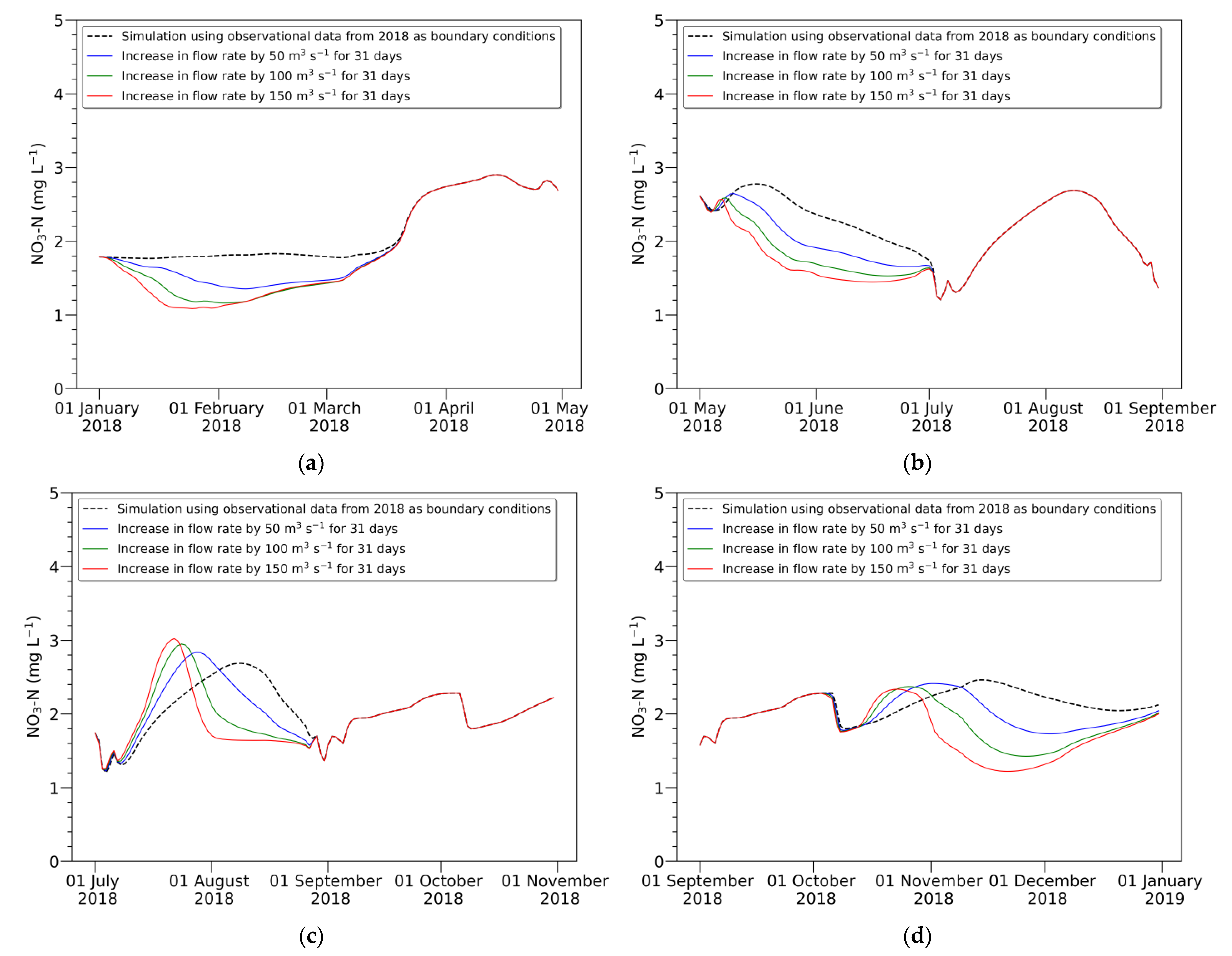
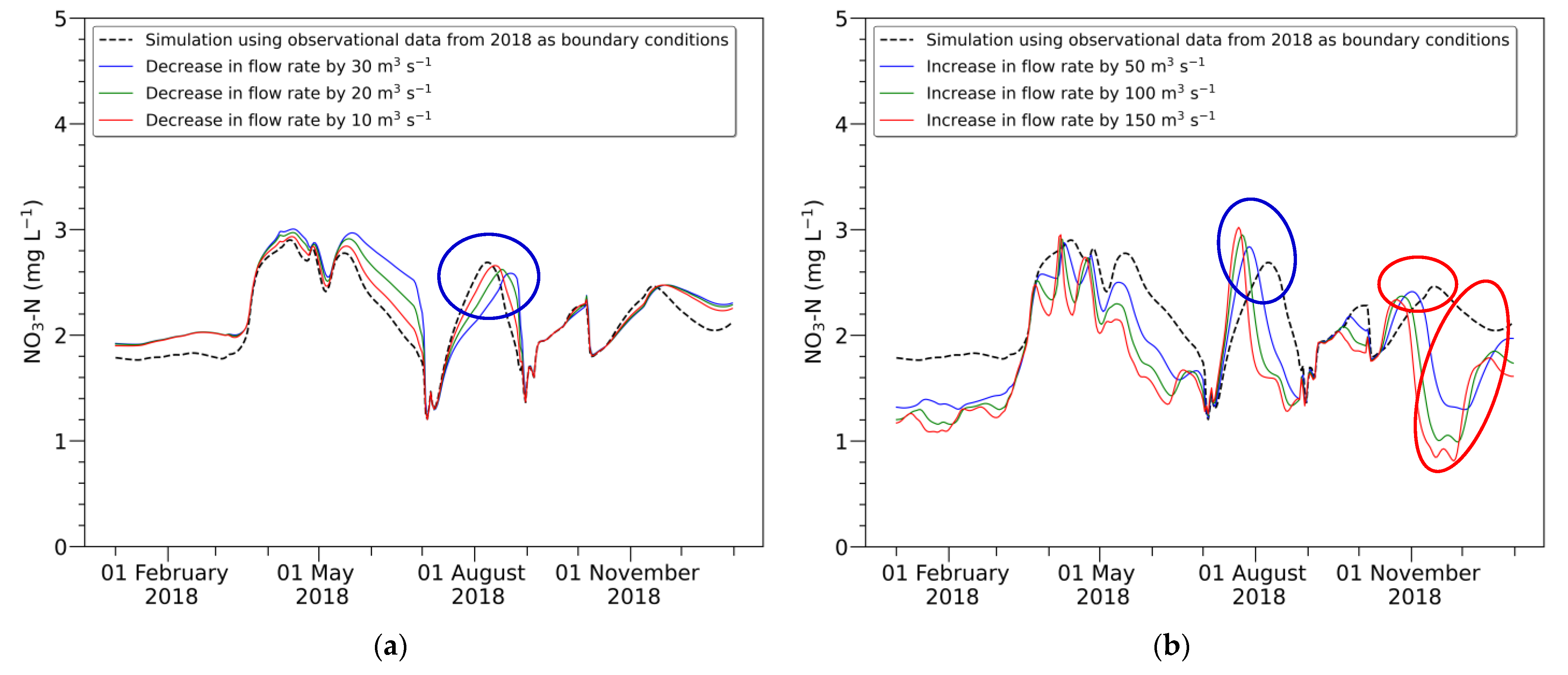
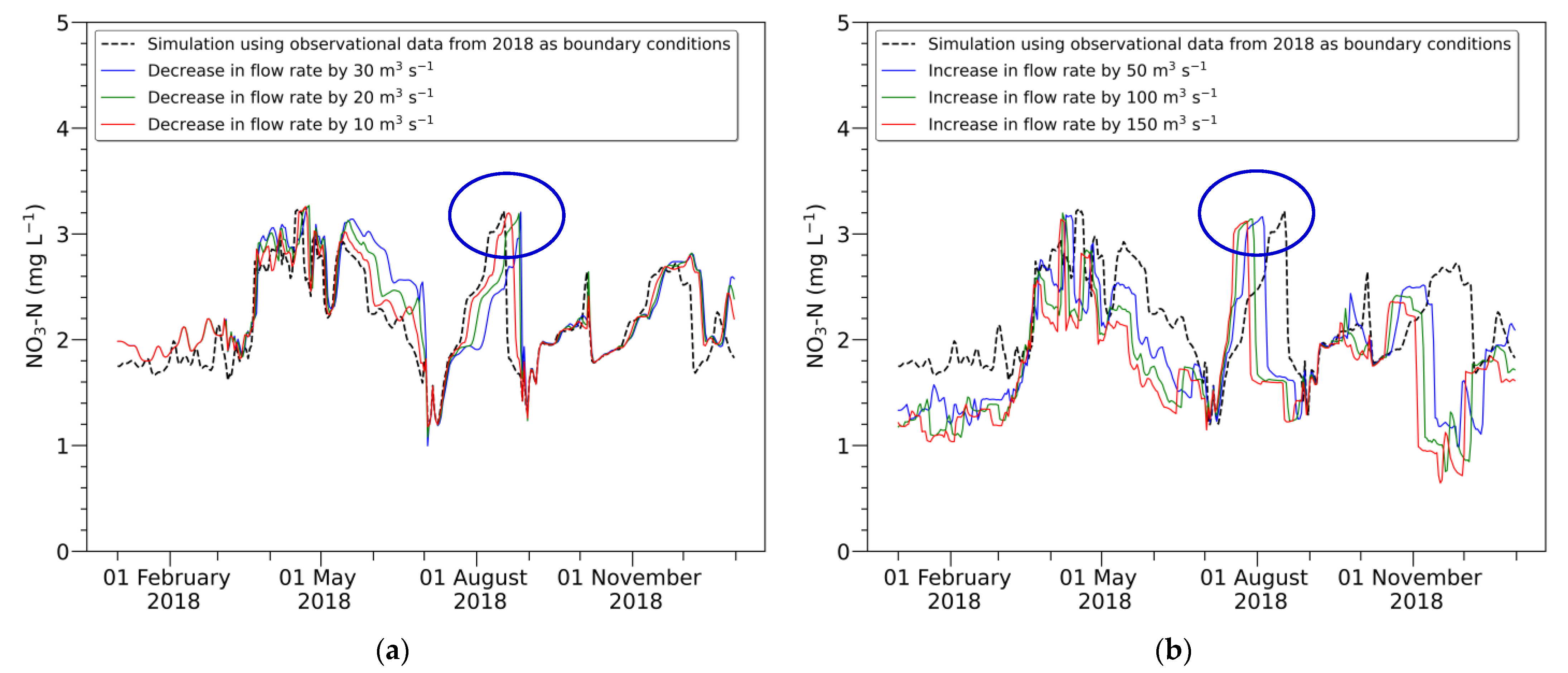
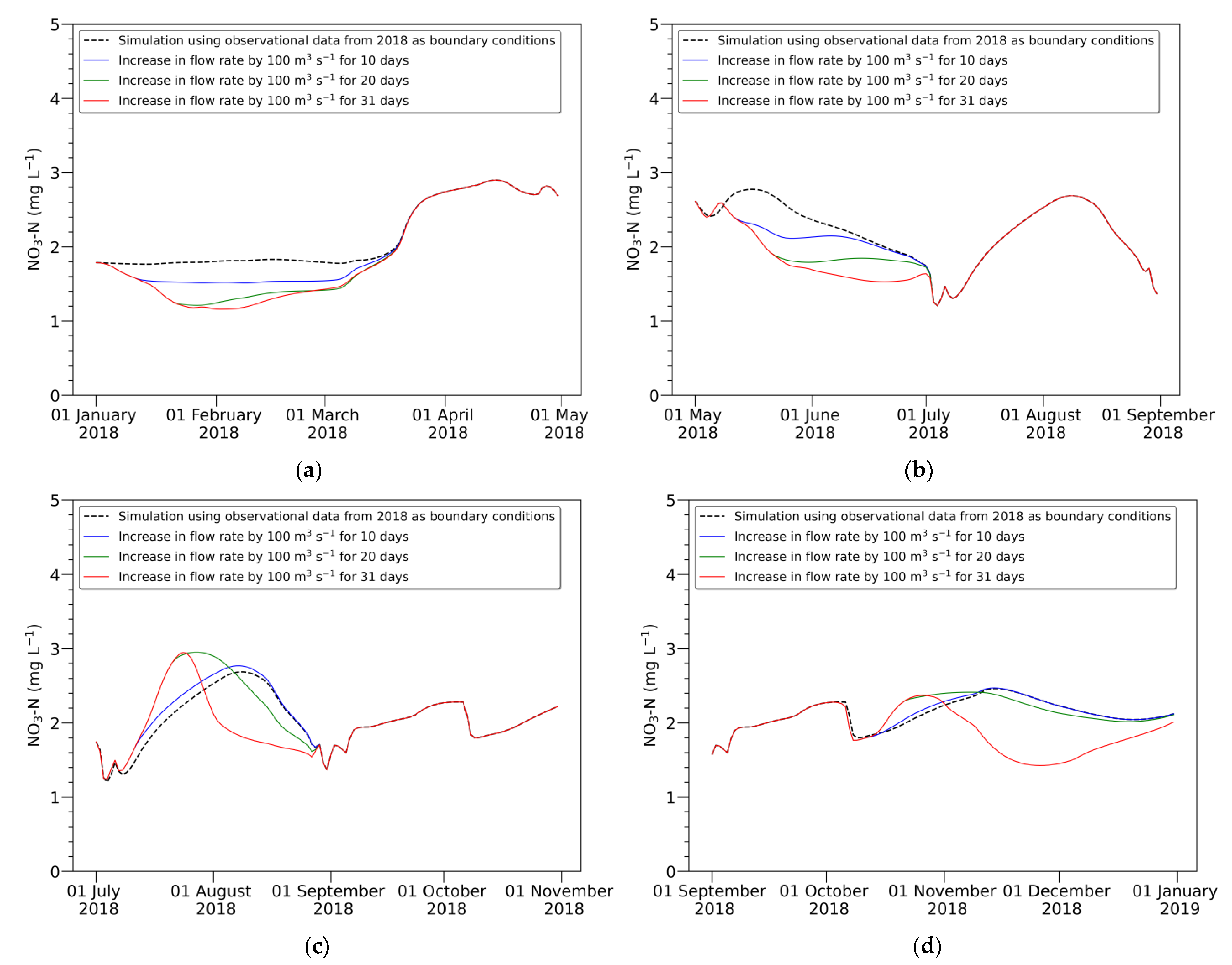
3.2. Scenario-Based NO3-N Dynamics

3.2.1. Variation in Water Quantity

Simulations under Scenarios 1–6 indicated changes in the concentration of NO3-N in cross section 416 caused by variations in the flow rate most upstream for the whole period (365 days), as shown in Figure 8. The black graph in Figure 8 shows the NO3-N concentration simulated using the observational data from 2018 as boundary conditions. We compared the other graphs, which are simulation results achieved by variation in flow rate, to the black graph.
The results showed that increased flow rates at the upstream boundary led to a decrease in the NO3-N concentrations in cross section 416. However, different aspects were explored regarding the change in the NO3-N concentration only around July and August, as indicated by the blue ellipses in Figure 8. In other words, the peak concentration of NO3-N increased in the blue ellipses, although the flow rate increased at the upstream boundary. This reversal was brought about when the downstream NO3-N concentration sharply increased in the simulation result using observational data at the boundaries (black graph). Here, the increase in flow rate seems to have accelerated the dispersion of the NO3-N concentration downstream. The acceleration in the dispersion temporarily caused a rapid increase in the NO3-N concentration. This hypothesis can be supported by comparing Figure 8 with Figure 9, which shows the results simulated with the fixed dispersion coefficient of zero. In the blue ellipses of Figure 9, the increase in flow rate did not lead to an increase in NO3-N concentration, unlike in Figure 8, which shows the results simulated with the computed dispersion coefficients.
The effect of decreasing the NO3-N concentration was more considerably exerted by an increase in the flow rate when the NO3-N concentration downstream was decreasing than when it was increasing, as indicated by the red ellipses in Figure 8. As shown in Table 10, the flow rate that increased by 150 m3 s−1 brought about a reduction effect of only 5.1%. This effect was shown when the NO3-N concentration was increasing. On the other hand, the rate of reduction in the NO3-N concentration was much higher (60.3%) when the NO3-N concentration was decreasing.
Interestingly, we found that a fall in the NO3-N concentration was not proportional to a rise in the flow rate. In Figure 8, this point is demonstrated by the unequal changes in the NO3-N concentration corresponding to the equal-step increase in flow rate (e.g., change in concentration is high for flow variation from 0 m3 s−1 to 50 m3 s−1, but it is insignificant for the change from 100 m3 s−1 to 150 m3 s−1). In any case, ever-increasing flow rates under Scenarios 4–6 do not match the reservoir operations in practice, because this may lead to a shortage of water supply. That is why we considered Scenarios 7–42, where the flow rates were increased at the upstream boundary temporarily instead of for the whole period (365 days).
The overall results obtained by the simulation under Scenarios 7–42 showed that the larger the flow rate, or the longer duration of the increase in flow rate, the more significant the reducing effect on the NO3-N concentration. Nonetheless, the results showed slight differences depending on when the flow rate started to increase. For instance, in Figure 10b and Figure 11b, it can be seen that the concentration of NO3-N decreased compared to the black graph, depending on the amount or the duration of increased flow. On the contrary, Figure 10c and Figure 11c show opposite results to Figure 10b and Figure 11b. The only difference between these cases was the time when the flow rate started to increase. Figure 10b and Figure 11b show the results achieved under the condition where the increase in flow rate began in May, when the NO3-N concentration was falling. On the other hand, in Figure 10c and Figure 11c, the flow rate increased at a time when the concentration of NO3-N was markedly rising.
In this regard, the current status of a river should be considered for decision making related to reservoir operations in terms of WQM. Specifically, decision makers should determine to what extent the flow rate released from a reservoir will be increased or decreased or when this action will be taken by considering the current status of the concentration of water pollutants. This will result in effective and efficient control of NO3-N downstream.

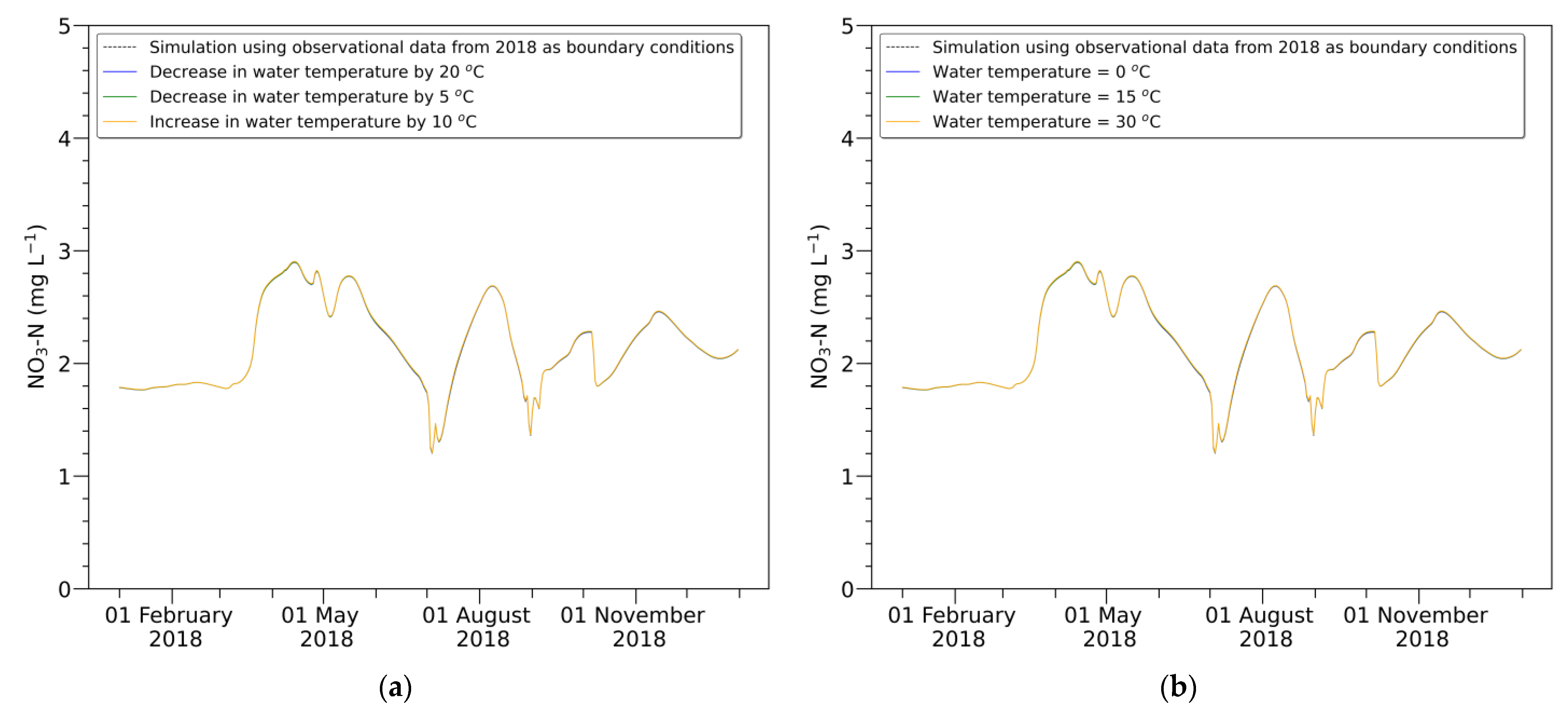
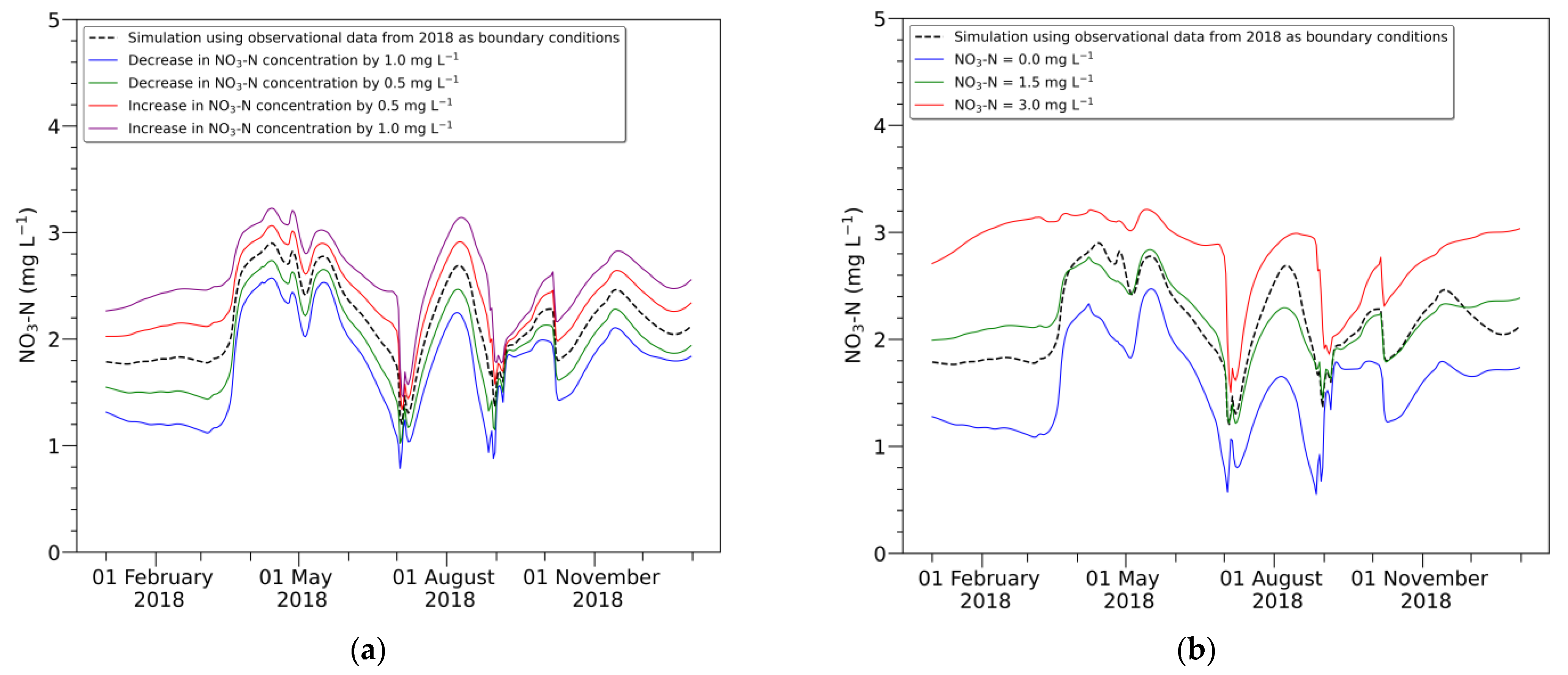
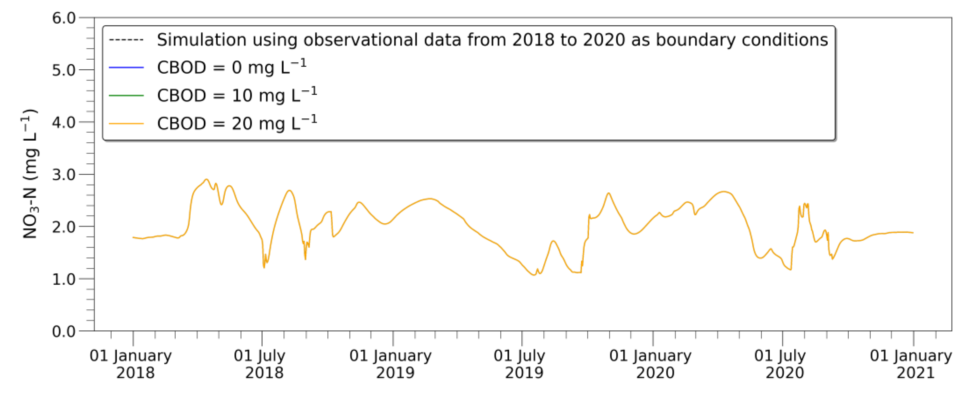
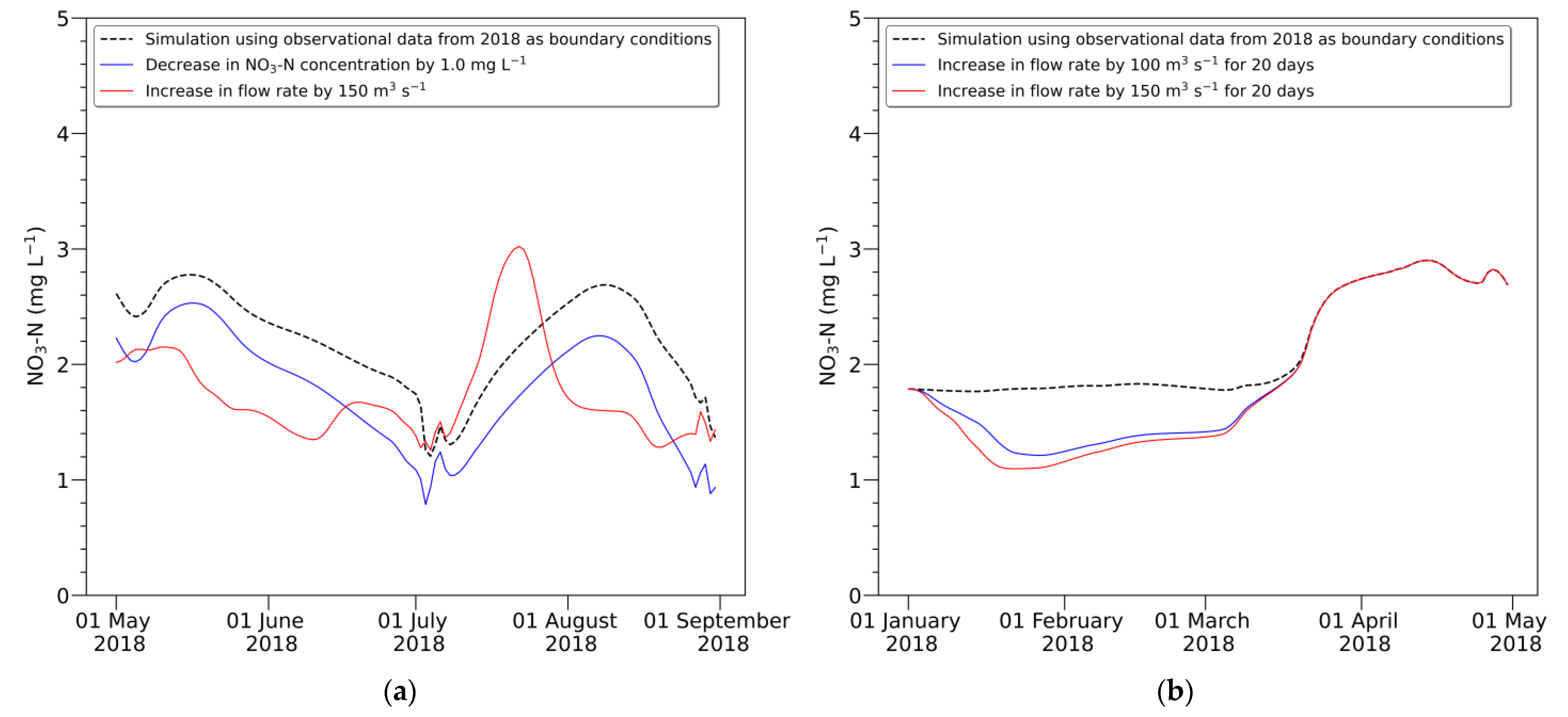
3.2.2. Variation in Water Quality

We learned from Scenarios 43–48 that variations in water temperature at the upstream boundary had little impact on the NO3-N concentration in cross section 416, as shown in Figure 12. This phenomenon seems to emerge because the water upstream is mixed with tributaries as the water flows downstream, and the water temperature of the river reaches equilibrium. This means that there is little impact on the concentration of NO3-N downstream only with the change in water temperature at the upstream boundary.
The simulation results under Scenarios 49–55 demonstrated that a marked variation in the NO3-N concentration occurred downstream if the concentration of NO3-N increased or decreased at the upstream boundary, as shown in Figure 13. In other words, control over the NO3-N concentration itself in the tributaries or the upper reaches of a river would be highly effective in controlling the concentration of NO3-N downstream. However, the amount of variation in the downstream NO3-N concentration may increase or decrease depending not only on the change in the upstream NO3-N concentration but also on the current status of the river, such as flow rate and water temperature. Therefore, the control method for NO3-N should be adopted in consideration of the current status in the target area. This sufficient consideration for the downstream status enables the establishment of effective strategies for controlling the downstream NO3-N concentration with a water quality model.

3.3. Guidelines for Design of Strategies to Control NO3-N Downstream

Effective strategies can be devised to control the downstream NO3-N concentration based on the simulation results of the Scenarios of this study. Guidelines for the design of strategies can be suggested using the control methods of the flow rate or the NO3-N concentration at the upstream boundary, which was proven effective under the Scenarios. The primary purpose of control methods should be carefully considered before employing the methods. The purpose can include control of the peak concentration or the overall average concentration of downstream NO3-N.
Specifically, the control method of the NO3-N concentration itself at the upstream boundary is much more practical for decreasing the highest concentration of NO3-N downstream than a change in the flow rate at the upstream boundary. This can be demonstrated in Figure 14a, which shows conditions of both decreasing and increasing concentrations of NO3-N in 2018 (black graph). The blue graph shows the variation in the NO3-N concentration in cross section 416 when the NO3-N concentration decreased by 1.0 mg L−1 at the upstream boundary. The red graph shows the simulation result achieved by a flow rate increase of 150 m3 s−1 at the upstream boundary. We could clearly observe that the peak concentration in the blue graph was lower than the peak in the red graph when the NO3-N concentration was increasing (July–August 2018). Contrastingly, when the NO3-N concentration was decreasing (May–June 2018), we could produce the effect of decreasing the downstream NO3-N concentration by increasing the flow rate more than by reducing the NO3-N concentration at the upstream boundary.
Nonetheless, a large flow rate is not always fully effective. Figure 14b shows that there is a slight difference in making the downstream NO3-N concentration decrease between an increase in flow rate of 172.8 million m3 (100 m3 s−1 for 20 days, the blue graph) and of 259.2 million m3 (150 m3 s−1 for 20 days, the red graph). The lowest concentrations of NO3-N were 1.212 mg L−1 (on 27 January) and 1.097 mg L−1 (on 22 January) in the blue and red graphs, respectively, with a difference of only 0.115 mg L−1.

4. Discussion

The simulation results showed how the downstream NO3-N concentration would respond depending on variation in the quantity and quality of water upstream. With these results, general guidelines for strategies to control downstream NO3-N can be suggested with the control methods for the peak concentration and the overall average concentration of NO3-N. The peak concentration of downstream NO3-N can be directly controlled by limiting the concentration of NO3-N in the tributaries or the upper reaches of a river. Control of the upstream flow rate is a viable strategy in terms of control over the overall average concentration of downstream NO3-N when its concentration is decreasing. Notably, the strategy related to water quantity can be effectively implemented by deciding how much the flow rate should be increased after performing a quantitative analysis of the impact on the control of the downstream NO3-N concentration. These strategies would be implemented by a combination of joint operations of the reservoirs with SWF and simulation results with the water quality model.
As mentioned earlier, the methodology presented in this study can be used in further research for the indirect regulation of HABs in rivers by controlling the NO3-N concentration. Since HABs are produced by various factors such as climate, aquatic environments, etc., many researchers have tried to find the major drivers to predict HABs [25]. Several previous studies suggested that NO3-N is one of the key factors underlying HABs [12,13,14]. Accurate prediction of HABs is not easy because HABs can be produced or faded not only by chemical factors but also by biological processes [19,59,70]. However, for cases when NO3-N is determined to be a critical factor, appropriate countermeasures against HABs in a river can be introduced by predicting and controlling the NO3-N concentration, which is relatively easier to simulate than HABs.
However, some studies have surprisingly shown that a low concentration of NO3-N promotes HABs, although the effect could depend on the species of algae [12,71,72,73]. If these findings are linked with this study, HABs could be controlled by a reduction in the flow rate released from an upstream reservoir as in Scenarios 1–3 or by an increase in the NO3-N concentration of the released water as in Scenarios 51 and 52 (highly unusual scenarios and hardly possible in practice). Nevertheless, since the implementation of this strategy may lead to an increase in the downstream NO3-N concentration, an optimization process is necessary by considering an acceptable standard in the NO3-N concentration required for drinking water sourced from the river.
All the processes for water quality modelling, such as monitoring, analyzing, predicting, and controlling water quality parameters, are closely related to human health and the stability of aquatic ecosystems [74,75]. This study, however, focused on the modelling process for one water quality parameter (NO3-N). Further studies should be oriented toward sustainable development in terms of public health and ecological diversity and away from simply focusing on the water quality model. For instance, a water quality model would forecast NO3-N concentrations in a river. The simulation result could be used for judging whether the concentrations would exceed an acceptable level regarding public health. If exceeding the acceptable level, a decision should be made in advance to reduce the NO3-N concentrations in the river. A series of these processes would support the sustainable development of human life and aquatic ecosystems.
Moreover, we need to mention the hindrances to this study to be considered in further research. In this study, we tried to clearly understand NO3-N dynamics depending on the changes in water quantity and quality at the upstream boundary. However, since there were limitations on available data, we needed to make some assumptions. For example, the concentrations of NH4-N and NO2-N required in HEC-RAS were replaced with the measured concentration of NH3-N and zero, respectively [62,63,64,65,66,67]. Despite these reasonable assumptions based on observable facts, the developed model may still have uncertainty. Furthermore, the HEC-RAS model has not been widely used as a water quality model, although it has been frequently used for flow analysis. This would mean that it should be further validated as a water quality model. In this study, we attempted to develop the HEC-RAS model to simulate the NO3-N dynamics in the Nakdong River, but its suitability for simulating other water quality parameters should be further demonstrated. Additionally, we constructed a one-dimensional model with HEC-RAS, but a multi-dimensional model would be necessary for detailed analysis of critical locations (e.g., weirs close to water supply intakes, such as the Chilgok Weir in this study). This is because the fate and transport of NO3-N may tend to vary in a transverse or vertical direction and not only in a longitudinal direction as modelled in this study. Further studies could be conducted with consideration for adequate substitutes for the data that were not measured, the limitations of the HEC-RAS model as a water quality model, and the application of a multi-dimensional model.

5. Conclusions

We developed a one-dimensional process-based model to simulate the fate and transport of NO3-N using HEC-RAS for the upper reach of the Nakdong River in South Korea. Variations in the downstream NO3-N concentration were simulated by the developed model according to changes in water quantity and quality at the upstream boundary. For the monitoring station located near the Chilgok Weir, these simulation results were analyzed in comparison with the modelling result that was obtained using the observational data as boundary conditions without the change in water quantity and quality.
The main finding in connection with the control of water quality is that the change in the downstream NO3-N concentration was mostly achieved by direct control of the NO3-N concentration at the upstream boundary. In terms of the control on water quantity, we could create a more significant impact on the change in the downstream NO3-N concentration by increasing the flow rate at the upstream boundary. However, the reducing effect on the NO3-N concentration varied depending on how long the flow rate increased and the current status of the downstream NO3-N concentration. Therefore, strategic decisions on WQM should be made after predicting what effect will be achieved using a water quality model.
Based on the guidelines for the design of strategies for controlling the downstream NO3-N concentration, we learned that the unilateral decision between water quantity and quality at the upstream boundary would not be best for the improvement in downstream water quality. In this respect, further research can be conducted on the optimal operation of reservoirs in consideration of both water quantity and quality. This optimization process can be accelerated together with a surrogate model for water quality based on a broad spectrum of scenarios.

Author Contributions

Conceptualization, D.P.S., A.J. and J.K.; methodology, D.P.S., A.J. and J.K.; software, J.K.; validation, A.J. and J.K.; formal analysis, J.K.; investigation, A.J. and J.K.; data curation, J.K.; writing—original draft preparation, J.K.; writing—review and editing, D.P.S., P.L.M.G. and A.J.; visualization, J.K.; supervision, D.P.S., P.L.M.G. and A.J. All authors have read and agreed to the published version of the manuscript.

Funding

This research received no external funding. The APC was funded by Delft University of Technology.

Institutional Review Board Statement

Not applicable.

Informed Consent Statement

Not applicable.

Data Availability Statement

The raw data are publicly available at http://www.wamis.go.kr for hydraulic data (accessed on 14 March 2022), https://water.nier.go.kr for water quality data (accessed on 30 March 2022), and https://data.kma.go.kr for meteorological data (accessed on 18 April 2022).

Acknowledgments

We thank K-water (Korea Water Resources Corporation) for financially supporting the first author.

Conflicts of Interest

The authors declare no conflict of interest.

References

  1. UNESCO; UN-Water. United Nations World Water Development Report 2020: Water and Climate Change; UNESCO: Paris, France, 2020; Available online: https://www.unwater.org/publications/un-world-water-development-report-2020 (accessed on 28 September 2022).
  2. WHO. Guidelines for Drinking-Water Quality: Fourth Edition Incorporating the First and Second Addenda, 4th ed.; World Health Organization: Geneva, Switzerland, 2022; Available online: https://www.who.int/publications/i/item/9789240045064 (accessed on 22 September 2022).
  3. Celikkol, S.; Fortin, N.; Tromas, N.; Andriananjamanantsoa, H.; Greer, C.W. Bioavailable Nutrients (N and P) and Precipitation Patterns Drive Cyanobacterial Blooms in Missisquoi Bay, Lake Champlain. Microorganisms 2021, 9, 2097. [Google Scholar] [CrossRef] [PubMed]
  4. Ward, M.H.; deKok, T.M.; Levallois, P.; Brender, J.; Gulis, G.; Nolan, B.T.; VanDerslice, J. Workgroup Report: Drinking-Water Nitrate and Health—Recent Findings and Research Needs. Environ. Health Perspect. 2005, 113, 1607–1614. [Google Scholar] [CrossRef] [PubMed] [Green Version]
  5. Danaraj, J.; Ushani, U.; Packiavathy, S.V.; Dharmadhas, J.S.; Karuppiah, T.; Anandha Kumar, S.; Aooj, E.S. Climate Change Impacts of Nitrate Contamination on Human Health. In Climate Change Impact on Groundwater Resources: Human Health Risk Assessment in Arid and Semi-Arid Regions; Panneerselvam, B., Pande, C.B., Muniraj, K., Balasubramanian, A., Ravichandran, N., Eds.; Springer International Publishing: Cham, Switzerland, 2022; pp. 257–278. [Google Scholar]
  6. Ward, M.H.; Jones, R.R.; Brender, J.D.; de Kok, T.M.; Weyer, P.J.; Nolan, B.T.; Villanueva, C.M.; van Breda, S.G. Drinking Water Nitrate and Human Health: An Updated Review. Int. J. Environ. Res. Public Health 2018, 15, 1557. [Google Scholar] [CrossRef] [PubMed] [Green Version]
  7. Lee, C.-M.; Hamm, S.-Y.; Cheong, J.-Y.; Kim, K.; Yoon, H.; Kim, M.; Kim, J. Contribution of Nitrate-Nitrogen Concentration in Groundwater to Stream Water in an Agricultural Head Watershed. Environ. Res. 2020, 184, 109313. [Google Scholar] [CrossRef] [PubMed]
  8. Nakagawa, K.; Amano, H.; Asakura, H.; Berndtsson, R. Spatial Trends of Nitrate Pollution and Groundwater Chemistry in Shimabara, Nagasaki, Japan. Environ. Earth Sci. 2016, 75, 234. [Google Scholar] [CrossRef] [Green Version]
  9. Musacchio, A.; Re, V.; Mas-Pla, J.; Sacchi, E. EU Nitrates Directive, from Theory to Practice: Environmental Effectiveness and Influence of Regional Governance on Its Performance. Ambio 2020, 49, 504–516. [Google Scholar] [CrossRef] [PubMed] [Green Version]
  10. Elzain, H.E.; Chung, S.Y.; Senapathi, V.; Sekar, S.; Lee, S.Y.; Priyadarsi, R.D.; Hassan, A.; Sabarathinam, C. Comparative Study of Machine Learning Models for Evaluating Groundwater Vulnerability to Nitrate Contamination. Ecotoxicol. Environ. Saf. 2022, 229, 113061. [Google Scholar] [CrossRef]
  11. Yang, L.; Yu, X. A Review of Development and Application on River Comprehensive Water Quality Model QUAL2K. In IOP Conference Series: Earth and Environmental Science; IOP Publishing: Bristol, UK, 2018. [Google Scholar]
  12. Kim, J.; Jonoski, A.; Solomatine, D.P. A Classification-Based Machine Learning Approach to the Prediction of Cyanobacterial Blooms in Chilgok Weir, South Korea. Water 2022, 14, 542. [Google Scholar] [CrossRef]
  13. Park, Y.; Lee, H.K.; Shin, J.-K.; Chon, K.; Kim, S.; Cho, K.H.; Kim, J.H.; Baek, S.-S. A Machine Learning Approach for Early Warning of Cyanobacterial Bloom Outbreaks in a Freshwater Reservoir. J. Environ. Manag. 2021, 288, 112415. [Google Scholar] [CrossRef]
  14. Zhao, W.X.; Li, Y.Y.; Jiao, Y.J.; Zhou, B.; Vogt, R.D.; Liu, H.L.; Ji, M.; Ma, Z.; Li, A.D.; Zhou, B.H.; et al. Spatial and Temporal Variations in Environmental Variables in Relation to Phytoplankton Community Structure in a Eutrophic River-Type Reservoir. Water 2017, 9, 754. [Google Scholar] [CrossRef]
  15. Paerl, H.W.; Otten, T.G. Harmful Cyanobacterial Blooms: Causes, Consequences, and Controls. Microb. Ecol. 2013, 65, 995–1010. [Google Scholar] [CrossRef] [PubMed]
  16. Falconer, I.R.; Humpage, A.R. Health Risk Assessment of Cyanobacterial (Blue-Green Algal) Toxins in Drinking Water. Int. J. Environ. Res. Public Health 2005, 2, 43–50. [Google Scholar] [CrossRef] [PubMed] [Green Version]
  17. Ho, L.; Goethals, P. Research Hotspots and Current Challenges of Lakes and Reservoirs: A Bibliometric Analysis. Scientometrics 2020, 124, 603–631. [Google Scholar] [CrossRef] [Green Version]
  18. Park, H.-K.; Lee, H.-J.; Heo, J.; Yun, J.-H.; Kim, Y.-J.; Kim, H.-M.; Hong, D.-G.; Lee, I.-J. Deciphering the Key Factors Determining Spatio-Temporal Heterogeneity of Cyanobacterial Bloom Dynamics in the Nakdong River with Consecutive Large Weirs. Sci. Total Environ. 2021, 755, 143079. [Google Scholar] [CrossRef]
  19. Park, Y.; Pyo, J.; Kwon, Y.S.; Cha, Y.; Lee, H.; Kang, T.; Cho, K.H. Evaluating Physico-Chemical Influences on Cyanobacterial Blooms Using Hyperspectral Images in Inland Water, Korea. Water Res. 2017, 126, 319–328. [Google Scholar] [CrossRef] [PubMed]
  20. Song, H.; Lynch, M.J. Restoration of Nature or Special Interests? A Political Economy Analysis of the Four Major Rivers Restoration Project in South Korea. Crit. Criminol. 2018, 26, 251–270. [Google Scholar] [CrossRef]
  21. Romo, S.; Soria, J.; Fernandez, F.; Ouahid, Y.; Baron-Sola, A. Water Residence Time and the Dynamics of Toxic Cyanobacteria. Freshw. Biol. 2013, 58, 513–522. [Google Scholar] [CrossRef]
  22. Aguilar, J.; Van Andel, S.-J.; Werner, M.; Solomatine, D.P. Hydrodynamic and Water Quality Surrogate Modeling for Reservoir Operation. In Proceedings of the 11th International Conference on Hydroinformatics, New York, NY, USA, 17–21 August 2014. [Google Scholar]
  23. Engel, B.; Storm, D.; White, M.; Arnold, J.; Arabi, M. A Hydrologic/Water Quality Model Application Protocol. J. Am. Water Resour. Assoc. 2007, 43, 1223–1236. [Google Scholar] [CrossRef]
  24. Ejigu, M.T. Overview of Water Quality Modeling. Cogent Eng. 2021, 8, 1891711. [Google Scholar] [CrossRef]
  25. Rousso, B.Z.; Bertone, E.; Stewart, R.; Hamilton, D.P. A Systematic Literature Review of Forecasting and Predictive Models for Cyanobacteria Blooms in Freshwater Lakes. Water Res. 2020, 182, 115959. [Google Scholar] [CrossRef]
  26. Srivastava, P.; McVair, J.N.; Johnson, T.E. Comparison of Process-Based and Artificial Neural Network Approaches for Streamflow Modeling in an Agricultural Watershed. J. Am. Water Resour. Assoc. 2006, 42, 545–563. [Google Scholar] [CrossRef]
  27. Razavi, S.; Tolson, B.A.; Burn, D.H. Review of Surrogate Modeling in Water Resources. Water Resour. Res. 2012, 48, W07401. [Google Scholar] [CrossRef]
  28. Costa, C.M.d.B.; Leite, I.R.; Almeida, A.K.; de Almeida, I.K. Choosing an Appropriate Water Quality Model-a Review. Environ. Monit. Assess. 2021, 193, 38. [Google Scholar] [CrossRef] [PubMed]
  29. Alam, M.J.; Dutta, D. Modelling of Nutrient Pollution Dynamics in River Basins: A Review with a Perspective of a Distributed Modelling Approach. Geosciences 2021, 11, 369. [Google Scholar] [CrossRef]
  30. Gunawardena, M.P.; Najim, M.M.M. Adapting Sri Lanka to Climate Change: Approaches to Water Modelling in the Upper Mahaweli Catchment Area. In Climate Change Research at Universities: Addressing the Mitigation and Adaptation Challenges; Leal Filho, W., Ed.; Springer International Publishing: Cham, Switzerland, 2017; pp. 95–115. [Google Scholar]
  31. Abed, B.S.; Daham, M.H.; Al-Thamiry, H.A. Assessment and Modelling of Water Quality along Al-Gharraf River (Iraq). J. Green Eng. 2020, 10, 13565–13579. [Google Scholar]
  32. Brunner, G.W. HEC-RAS River Analysis System User’s Manual Version 5.0; U.S. Army Corps of Engineers, Institute for Water Resources, Hydrologic Engineering Center: Davis, CA, USA, 2016; Available online: https://www.hec.usace.army.mil/software/hec-ras/documentation/HEC-RAS%205.0%20Users%20Manual.pdf (accessed on 20 January 2022).
  33. Teran-Velasquez, G.; Helm, B.; Krebs, P. Longitudinal River Monitoring and Modelling Substantiate the Impact of Weirs on Nitrogen Dynamics. Water 2022, 14, 189. [Google Scholar] [CrossRef]
  34. Taralgatti, P.D.; Pawar, R.S.; Pawar, G.S.; Nomaan, M.H.; Limkar, C.R. Water Quality Modeling of Bhima River by Using HEC-RAS Software. Int. J. Eng. Adv. Technol. 2020, 9, 2886–2889. [Google Scholar] [CrossRef]
  35. Abed, B.S.; Daham, M.H.; Ismail, A.H. Water Quality Modelling and Management of Diyala River and Its Impact on Tigris River. J. Eng. Sci. Technol. 2021, 16, 122–135. [Google Scholar]
  36. Ghafoor, J.; Forio, M.A.E.; Goethals, P.L.M. Spatially Explicit River Basin Models for Cost-Benefit Analyses to Optimize Land Use. Sustainability 2022, 14, 8953. [Google Scholar] [CrossRef]
  37. Lee, H.-J.; Park, H.-K.; Cheon, S.-U. Effects of Weir Construction on Phytoplankton Assemblages and Water Quality in a Large River System. Int. J. Environ. Res. Public Health 2018, 15, 2348. [Google Scholar] [CrossRef] [Green Version]
  38. Kim, D.-H.; Lee, S.-K.; Chun, B.-Y.; Lee, D.-H.; Hong, S.-C.; Jang, B.-K. Illness Associated with Contamination of Drinking Water Supplies with Phenol. J. Korean Med. Sci. 1994, 9, 218–223. [Google Scholar] [CrossRef] [PubMed] [Green Version]
  39. Jo, C.D.; Lee, C.G.; Kwon, H.G. Effects of Multifunctional Weir Construction on Key Water Quality Indicators: A Case Study in Nakdong River, Korea. Int. J. Environ. Sci. Technol. 2022, 19, 11843–11856. [Google Scholar] [CrossRef]
  40. Park, J.; Wang, D.; Lee, W.H. Evaluation of Weir Construction on Water Quality Related to Algal Blooms in the Nakdong River. Environ. Earth Sci. 2018, 77, 408. [Google Scholar] [CrossRef]
  41. Jeong, J.-W.; Kim, Y.-O.; Seo, S.B. Evaluating Joint Operation Rules for Connecting Tunnels between Two Multipurpose Dams. Hydrol. Res. 2020, 51, 392–405. [Google Scholar] [CrossRef]
  42. Park, J.C.; Um, M.-J.; Song, Y.-I.; Hwang, H.-D.; Kim, M.M.; Park, D. Modeling of Turbidity Variation in Two Reservoirs Connected by a Water Transfer Tunnel in South Korea. Sustainability 2017, 9, 993. [Google Scholar] [CrossRef] [Green Version]
  43. Lee, S.; Kim, J.; Noh, J.; Ko, I.H. Assessment of Selective Withdrawal Facility in the Imha Reservoir Using CE-QUAL-W2 Model. J. Korean Soc. Water Environ. 2007, 23, 228–235. [Google Scholar]
  44. Park, H.-S.; Chung, S.-W. Water Transportation and Stratification Modification in the Andong-Imha Linked Reservoirs System. J. Korean Soc. Water Environ. 2014, 30, 31–43. [Google Scholar] [CrossRef] [Green Version]
  45. Lee, J.; Bae, S.; Lee, D.-R.; Seo, D. Transportation Modeling of Conservative Pollutant in a River with Weirs-The Nakdong River Case. J. Korean Soc. Environ. Eng. 2014, 36, 821–827. [Google Scholar] [CrossRef] [Green Version]
  46. Bae, S.; Seo, D. Changes in Algal Bloom Dynamics in a Regulated Large River in Response to Eutrophic Status. Ecol. Model. 2021, 454, 109590. [Google Scholar] [CrossRef]
  47. Kim, D.; Shin, C. Algal Boom Characteristics of Yeongsan River Based on Weir and Estuary Dam Operating Conditions Using EFDC-NIER Model. Water 2021, 13, 2295. [Google Scholar] [CrossRef]
  48. Choi, H.-G.; Han, K.-Y. Development and Applicability Assessment of 1-D Water Quality Model in Nakdong River. KSCE J. Civ. Eng. 2014, 18, 2234–2243. [Google Scholar] [CrossRef]
  49. Leonard, B.P. A Stable and Accurate Convective Modelling Procedure Based on Quadratic Upstream Interpolation. Comput. Methods Appl. Mech. Eng. 1979, 19, 59–98. [Google Scholar] [CrossRef]
  50. Leonard, B.P. The ULTIMATE Conservative Difference Scheme Applied to Unsteady One-Dimensional Advection. Comput. Methods Appl. Mech. Eng. 1991, 88, 17–74. [Google Scholar] [CrossRef]
  51. Korea Legislation Research Institute. The Statutes of the Republic of Korea Home Page: River Act. Available online: https://elaw.klri.re.kr/eng_service/lawView.do?hseq=57588&lang=ENG (accessed on 28 September 2022).
  52. Kim, J.; Seo, D.; Jang, M.; Kim, J. Augmentation of Limited Input Data Using an Artificial Neural Network Method to Improve the Accuracy of Water Quality Modeling in a Large Lake. J. Hydrol. 2021, 602, 126817. [Google Scholar] [CrossRef]
  53. Korea Legislation Research Institute. The Statutes of the Republic of Korea Home Page: Act on the Investigation, Planning, and Management of Water Resources. Available online: https://elaw.klri.re.kr/eng_service/lawView.do?hseq=55436&lang=ENG (accessed on 28 September 2022).
  54. Korea Legislation Research Institute. The Statutes of the Republic of Korea Home Page: Water Environment Conservation Act. Available online: https://elaw.klri.re.kr/eng_service/lawView.do?hseq=54838&lang=ENG (accessed on 28 September 2022).
  55. Korea Legislation Research Institute. The Statutes of the Republic of Korea Home Page: Weather Act. Available online: https://elaw.klri.re.kr/eng_service/lawView.do?hseq=54691&lang=ENG (accessed on 28 September 2022).
  56. Cullinan, V.I.; May, C.W.; Brandenberger, J.M.; Judd, C.; Johnston, R.K. Development of an Empirical Water Quality Model for Stormwater Based on Watershed Land Use in Puget Sound; Space and Naval Warfare Systems Center, Marine Environmental Support Office: Bremerton, WA, USA, 2007; Available online: https://apps.dtic.mil/sti/citations/ADA519147 (accessed on 23 September 2022).
  57. James, R.T. Recalibration of the Lake Okeechobee Water Quality Model (LOWQM) to Extreme Hydro-Meteorological Events. Ecol. Model. 2016, 325, 71–83. [Google Scholar] [CrossRef]
  58. McIntyre, N.R.; Wheater, H.S. A Tool for Risk-Based Management of Surface Water Quality. Environ. Model. Softw. 2004, 19, 1131–1140. [Google Scholar] [CrossRef]
  59. Kim, J.; Lee, T.; Seo, D. Algal Bloom Prediction of the Lower Han River, Korea Using the EFDC Hydrodynamic and Water Quality Model. Ecol. Model. 2017, 366, 27–36. [Google Scholar] [CrossRef]
  60. Yi, H.-S.; Park, S.; An, K.-G.; Kwak, K.-C. Algal Bloom Prediction Using Extreme Learning Machine Models at Artificial Weirs in the Nakdong River, Korea. Int. J. Environ. Res. Public Health 2018, 15, 2078. [Google Scholar] [CrossRef] [Green Version]
  61. Zhang, Z.; Johnson, B.E. Aquatic Nutrient Simulation Modules (NSMs) Developed for Hydrologic and Hydraulic Models; U.S. Army Engineer Research and Development Center, Environmental Laboratory: Vicksburg, MS, USA, 2016; Available online: https://erdc-library.erdc.dren.mil/jspui/bitstream/11681/10112/1/ERDC-EL-TR-16-1.pdf (accessed on 20 January 2022).
  62. Meybeck, M. Carbon, Nitrogen, and Phosphorus Transport by World Rivers. Am. J. Sci. 1982, 282, 401–450. [Google Scholar] [CrossRef]
  63. Park, J.; Sohn, S.; Kim, Y. Distribution Characteristics of Total Nitrogen Components in Streams by Watershed Characteristics. J. Korean Soc. Water Environ. 2014, 30, 503–511. [Google Scholar] [CrossRef] [Green Version]
  64. Bhuyan, K.J.; Saharia, P.K.; Sarma, D.; Bhagawati, K.; Baishya, S.; Hazarika, S.R. Effect of Periphyton (Streblus Asper Lour.) Assemblage on Water quality Parameters and Growth Perfomance of Jayanti Rohu and Amur Common Carp in the Aquaculture System. J. Krishi Vigyan 2020, 9, 74–80. [Google Scholar] [CrossRef]
  65. Mihale, M.J. Nitrogen and Phosphorus Dynamics in the Waters of the Great Ruaha River, Tanzania. J. Water Resour. Ocean Sci. 2015, 4, 59–71. [Google Scholar] [CrossRef] [Green Version]
  66. Rus, D.L.; Patton, C.J.; Mueller, D.K.; Crawford, C.G. Assessing Total Nitrogen in Surface-Water Samples: Precision and Bias of Analytical and Computational Methods; U.S. Department of the Interior, U.S. Geological Survey: Reston, VA, USA, 2012. Available online: https://pubs.usgs.gov/sir/2012/5281 (accessed on 15 September 2022).
  67. Hem, J.D. Study and Interpretation of the Chemical Characteristics of Natural Water; U.S. Department of the Interior, U.S. Geological Survey: Alexandria, VA, USA, 1985. [Google Scholar]
  68. Daggupati, P.; Pai, N.; Ale, S.; Douglas-Mankin, K.R.; Zeckoski, R.W.; Jeong, J.; Parajuli, P.B.; Saraswat, D.; Youssef, M.A. A Recommended Calibration and Validation Strategy for Hydrologic and Water Quality Models. T. Asabe 2015, 58, 1705–1719. [Google Scholar] [CrossRef]
  69. Moriasi, D.N.; Gitau, M.W.; Pai, N.; Daggupati, P. Hydrologic and Water Quality Models: Performance Measures and Evaluation Criteria. T. Asabe 2015, 58, 1763–1785. [Google Scholar] [CrossRef] [Green Version]
  70. Reynolds, C.S. The Ecology of Phytoplankton; Cambridge University Press: New York, NY, USA, 2006. [Google Scholar]
  71. Ferber, L.R.; Levine, S.N.; Lini, A.; Livingston, G.P. Do Cyanobacteria Dominate in Eutrophic Lakes Because They Fix Atmospheric Nitrogen? Freshwater Biol. 2004, 49, 690–708. [Google Scholar] [CrossRef]
  72. Weyhenmeyer, G.A.; Jeppesen, E.; Adrian, R.; Arvola, L.; Blenckner, T.; Jankowski, T.; Jennings, E.; Nõges, P.; Nõges, T.; Straile, D. Nitrate-Depleted Conditions on the Increase in Shallow Northern European Lakes. Limnol. Oceanogr. 2007, 52, 1346–1353. [Google Scholar] [CrossRef] [Green Version]
  73. Talib, A.; Recknagel, F.; Cao, H.; van der Molen, D.; Abu Hasan, Y. Use of Hybrid EA Models for the Prediction of Chlorophyll-a and Phytoplankton Functional Groups Abundance in Two Shallow Lakes. Malays. J. Math. Sci. 2008, 2, 11–28. [Google Scholar]
  74. Ustaoglu, F.; Tas, B.; Tepe, Y.; Topaldemir, H. Comprehensive Assessment of Water Quality and Associated Health Risk by Using Physicochemical Quality Indices and Multivariate Analysis in Terme River, Turkey. Environ. Sci. Pollut. Res. 2021, 28, 62736–62754. [Google Scholar] [CrossRef]
  75. Forio, M.A.E.; Goethals, P.L.M. An Integrated Approach of Multi-Community Monitoring and Assessment of Aquatic Ecosystems to Support Sustainable Development. Sustainability 2020, 12, 5603. [Google Scholar] [CrossRef]
Figure 1. Location of the study area.
Water 15 00247 g001
Figure 2. Location of the monitoring stations. (a) Stations for hydraulic data and two weather stations; (b) stations for water quality data and two weather stations.
Water 15 00247 g002
Figure 3. Graph showing the changes in the downstream NO3-N concentration caused by changes in the CBOD concentration at all the boundary conditions.
Water 15 00247 g003
Figure 4. Hydrographs showing the difference between simulation and observation for calibration. (a) Cross section 620; (b) cross section 559; (c) cross section 505; (d) cross section 437.
Water 15 00247 g004
Figure 5. Hydrographs showing the difference between simulation and observation for validation. (a) Cross section 620; (b) cross section 559; (c) cross section 505; (d) cross section 437.
Water 15 00247 g005
Figure 6. Graphs showing the difference between simulation and observation of the NO3-N concentration for calibration. (a) Cross section 658; (b) cross section 620; (c) cross section 559; (d) cross section 517; (e) cross section 503; (f) cross section 459; (g) cross section 427; (h) cross section 416.
Water 15 00247 g006aWater 15 00247 g006b
Figure 7. Graphs showing the difference between simulation and observation of the NO3-N concentration for validation. (a) Cross section 658; (b) cross section 620; (c) cross section 559; (d) cross section 517; (e) cross section 503; (f) cross section 459; (g) cross section 427; (h) cross section 416.
Water 15 00247 g007aWater 15 00247 g007b
Figure 8. Changes in the NO3-N concentration in cross section 416 caused by variations in flow rate at the upstream boundary for 365 days. The black graph shows the NO3-N concentration simulated using the observational data from 2018 as boundary conditions. The dispersion coefficient was automatically computed in HEC-RAS. (a) Changes in the NO3-N concentration by a decrease in flow rates (Scenarios 1–3); (b) changes in the NO3-N concentration by an increase in flow rates (Scenarios 4–6).
Water 15 00247 g008
Figure 9. Changes in the NO3-N concentration in cross section 416 caused by variations in flow rate at the upstream boundary for 365 days. The black graph shows the NO3-N concentration simulated using the observational data from 2018 as boundary conditions. The dispersion coefficient was set to zero. (a) Changes in the NO3-N concentration by a decrease in flow rates (Scenarios 1–3); (b) changes in the NO3-N concentration by an increase in flow rates (Scenarios 4–6).
Water 15 00247 g009
Figure 10. Changes in the NO3-N concentration in cross section 416 caused by variations in flow rate (50, 100, and 150 m3 s−1) at the upstream boundary for 31 days. The black graph shows the NO3-N concentration simulated using the observational data from 2018 as boundary conditions. The change in flow rate occurred in: (a) January; (b) May; (c) July; and (d) October.
Water 15 00247 g010
Figure 11. Changes in the NO3-N concentration in cross section 416 caused by variations in flow rate (100 m3 s−1) at the upstream boundary for 10, 20, and 31 days. The black graph shows the NO3-N concentration simulated using the observational data from 2018 as boundary conditions. The change in flow rate occurred in: (a) January; (b) May; (c) July; and (d) October.
Water 15 00247 g011
Figure 12. Changes in the NO3-N concentration in cross section 416 caused by variations in water temperature at the upstream boundary. The black graphs show results simulated using the observational data from 2018 as boundary conditions. (a) Changes in the NO3-N concentration by a decrease or increase in water temperature (Scenarios 43–45); (b) changes in the NO3-N concentration by constant water temperature (Scenarios 46–48).
Water 15 00247 g012
Figure 13. Changes in the NO3-N concentration in cross section 416 caused by variations in the NO3-N concentration at the upstream boundary. The black graphs show results simulated using the observational data from 2018 as boundary conditions. (a) Changes in the NO3-N concentration by a decrease or increase in the NO3-N concentration (Scenarios 49–52); (b) changes in the NO3-N concentration by a constant concentration of NO3-N (Scenarios 53–55).
Water 15 00247 g013
Figure 14. Changes in the NO3-N concentration in cross section 416 caused by a decrease in the NO3-N concentration at the upstream boundary or an increase in flow rate at the upstream boundary. The black graphs show the result simulated using the observational data from 2018 as boundary conditions. (a) Changes in the NO3-N concentration by a decrease in the NO3-N concentration (blue graph) or an increase in flow rate (red graph); (b) changes in the NO3-N concentration by an increase in flow rate of 100 m3 s−1 (blue graph) and 150 m3 s−1 (red graph) for 20 days.
Water 15 00247 g014
Table 1. Details about Andong and Imha reservoirs.
ReservoirAndongImha
Area of catchment (km2)1584.01361.0
Height of dam (m)83.073.0
Length of dam (m)612.0515.0
Normal high water level (mamsl)160.0163.0
Effective storage volume (106 m3)1000.0424.0
Table 2. Details about Sangju, Nakdan, Gumi, and Chilgok weirs.
WeirSangjuNakdanGumiChilgok
Area of catchment (km2)7407.09221.09557.011,040.0
Height (m)11.011.511.011.8
Length (m)335.0286.0374.3400.0
Water level for management (mamsl)47.040.032.525.5
Storage volume (106 m3)27.434.752.775.3
Table 3. Mean, minimum, and maximum values of the observational data (flow rate and NO3-N) in the cross sections for model calibration (2019) and validation (2020).
Data
(Unit)
Cross Section NumberCalibration (2019)Validation (2020)
MeanMinimumMaximumMeanMinimumMaximum
Flow rate
(m3 s−1)
62048.855.06976.4594.4110.381909.73
55976.7817.301675.61173.6818.842499.44
50598.874.273031.83212.0523.783632.07
437116.0924.064677.58270.6221.504495.12
NO3-N
(mg L−1)
6581.3130.6793.0381.4451.0552.453
6201.3980.2403.0581.5471.0952.512
5591.7500.8072.8721.8440.9002.924
5171.6880.6512.9351.8400.9932.858
5031.7600.7982.8031.8840.8692.890
4591.6930.7222.8711.9171.1792.957
4271.8860.6243.0992.0111.0553.095
4161.8410.7323.0272.0091.0662.986
Table 4. Main parameters related to NO3-N dynamics provided in HEC-RAS.
ParameterDescriptionDefault Value
Beta 3Rate constant: DON→NH4-N0.020
Beta 1Rate constant: NH4-N→NO2-N0.100
Beta 2Rate constant: NO2-N→NO3-N0.200
Sigma 4Settling rate (DON)0.001
KNRNitrification inhibition coefficient0.600
Table 5. Scenarios constructed for an understanding of NO3-N dynamics downstream.
Components *Increment/DecrementPeriodStart DateScenario
Water
quantity
Flow rate
(m3 s−1)
−30365 days1 JanuaryScenario 1
−20Scenario 2
−10Scenario 3
+50Scenario 4
+100Scenario 5
+150Scenario 6
+50
+100
+150
10 days
20 days
31 days
1 January
1 May
1 July
1 October
Scenario 7–42
Water
quality
Water
temperature
(°C)
–20365 days1 JanuaryScenario 43
−5Scenario 44
+10Scenario 45
Constant 0Scenario 46
Constant 15Scenario 47
Constant 30Scenario 48
NO3-N
(mg L−1)
−1.0365 days1 JanuaryScenario 49
−0.5Scenario 50
+0.5Scenario 51
+1.0Scenario 52
Constant 0.0Scenario 53
Constant 1.5Scenario 54
Constant 3.0Scenario 55
Note: * The components belong to the boundary conditions at the upstream boundary.
Table 6. Manning’s roughness coefficients for the hydraulic unsteady model.
Cross Section NumberManning Roughness Coefficient
411–4670.024
468–6720.026
673–6890.028
Table 7. Hydraulic model performance for unsteady flow.
Calibration/ValidationCross Section NumberR2NSEPBIAS (%)Performance
Calibration6200.9560.612−10.3 Satisfactory
5590.9750.9452.0 Very Good
5050.9670.96210.5 Satisfactory
4370.9290.86611.7 Satisfactory
Validation6200.8750.870−9.4 Good
5590.9480.9376.5 Good
5050.9520.9189.8 Good
4370.9630.91716.7 Not Satisfactory
Table 8. Mean values of both the observational data and the simulation results for the water quality parameters from 2019 (calibration) to 2020 (validation).
Water Quality Parameter
(Unit)
Cross Section Number
658620559517503459427416
Water temperature
(°C)
Observation15.014.516.416.715.716.217.415.7
Simulation13.812.812.512.612.012.812.412.1
DO
(mg L−1)
Observation10.610.510.611.010.910.410.810.3
Simulation10.610.610.810.811.010.810.911.1
DON
(mg L−1)
Observation0.4830.4240.4180.4280.3590.3750.4250.379
Simulation0.4100.4110.3970.4100.4020.4200.4180.416
NH4-N
(mg L−1)
Observation0.0620.0480.0550.0450.0530.0500.0770.091
Simulation0.0450.0430.0440.0370.0330.0410.0330.032
NO3-N
(mg L−1)
Observation1.3791.4731.7981.7651.8221.8101.9491.925
Simulation1.3101.3241.6641.7091.7721.8471.8991.917
Table 9. Model performance for NO3-N.
Calibration/ValidationCross Section NumberR2NSEPBIAS (%)Performance
Calibration6580.7890.7505.7Very Good
6200.4380.30110.3Not Satisfactory
5590.7660.6679.5Very Good
5170.8490.8013.5Very Good
5030.8720.8283.7Very Good
4590.8950.803−5.0Very Good
4270.8160.7320.5Very Good
4160.8520.777−1.7Very Good
Validation6580.6210.4784.4Satisfactory
6200.366−0.15510.0Not Satisfactory
5590.4940.4425.7Satisfactory
5170.6520.6402.8Good
5030.6110.6051.8Good
4590.7500.7490.4Very Good
4270.6060.5754.5Good
4160.7910.7642.4Very Good
Table 10. Example, taken from the red ellipses in Figure 8b, of the change in NO3-N concentration produced by an increase in flow rate.
Flow RateNO3-N
Increment
(m3 s−1)
Rate of Increment
(%)
Concentration
(mg L−1)
DateReduction in Concentration
(mg L−1)
Rate of Reduction
(%)
0-2.46314 November--
5033.32.4141 November0.0492.0
10066.72.37126 October0.0913.7
150100.02.33723 October0.1265.1
0-2.04621 December--
5033.31.2992 December0.74736.5
10066.70.99228 November1.05451.5
150100.00.81326 November1.23360.3
Disclaimer/Publisher’s Note: The statements, opinions and data contained in all publications are solely those of the individual author(s) and contributor(s) and not of MDPI and/or the editor(s). MDPI and/or the editor(s) disclaim responsibility for any injury to people or property resulting from any ideas, methods, instructions or products referred to in the content.

