Multivariate Regression Models for Predicting Pump-as-Turbine Characteristics

Abstract

Installing pumps as turbines (PaTs) in water distribution networks can recover otherwise wasted energy, as well as reduce leakage caused by high water pressure. However, a barrier to their implementation is the lack of information on their performance in turbine mode. Previous studies have proposed models to predict PaT characteristics based on pump best efficiency points (BEPs), using regressions with one or two dependent variables, or more complex artificial neural networks (ANNs). While ANNs were found to improve the accuracy of predictions, these models are known to be unstable with small datasets. Other types of regressions with multiple variables have not been explored. Furthermore, because only small datasets are available to train these models, multivariate regression methods could yield better results. The present study develops multivariate regression models to predict BEPs and characteristic curves of PaTs. A database of 145 BEPs and 196 characteristic curve PaT experimental records was compiled from previous literature. Twenty-four types of multi-variate regressions, as well as ANN were compared, with dimensioned and dimensionless versions of the datasets. The multivariate regression models consistently outperformed previous models, including ANN. The R² of the head and efficiency curves were 0.997 and 0.909, respectively. Results also showed that XGB regressors and a dimensionless dataset yielded the best-fit models overall. The high accuracy of the models, combined with their lower computational cost compared to ANN, make them a robust solution for selecting PaTs in practice.

1. Introduction

As the world increasingly recognizes the need for sustainable practices, great focus is given to energy generation and use. Among the essential services that municipalities provide, water is generally one of the most energy-intensive. Approximately 3.7 TWh of global energy use is associated with water supply, 2 TWh for distribution, and 1.7 TWh for wastewater treatment [1]. Furthermore, 30 to 60% of municipal expenses are related to the water industry [2]. It is, thus, clear that gains in water distribution energy efficiency and energy generation can lead to significant reductions in greenhouse gas (GHG) emissions and costs [3,4,5].

The safe and reliable operation of water distribution networks requires pressures to be controlled, often with pressure-reducing valves (PRVs). However, PRVs dissipate pressure through friction, wasting energy. Instead, energy can be recovered through micro-hydro turbines or pumps as turbines (PaTs) [6]. The former are generally more expensive than the latter [7]. PaTs are simply pumps operated in reverse, coupled with generators. The initial installation costs and GHG emissions are quickly offset with long-term savings and energy generation [8]. Still, one barrier to implementing PaTs remains. Manufacturers generally do not provide the characteristic attributes of pumps in reverse mode since this was not their initial intended application. Determining PaT characteristics can require expensive testing. Laboratory testing of PaTs can show different hydrodynamic and mechanical forcing scenarios and allow for tuning [9]. While lab results are reliable, they are time-consuming to achieve. Computational fluid dynamics (CFD) have also been applied in modeling PaT behavior with high accuracy [10,11], sometimes better than experimental results [9]. They enable the analysis of the effect of specific scenarios, e.g., transients [11], and pump characteristics, e.g., guide vane clocking positions [12], impeller geometry modifications [13], and variable rotational speed [14,15]. CFD nevertheless requires extensive time, resources, and computing power [16].

A less costly approach to predicting PaT performance has been the development of theoretical or empirical equations. Studies seeking to select the optimal PaT for a water distribution network, regularly employ these equations to estimate turbine performance based on known pump characteristics [6,17,18,19].

Stepanoff [20] was the first to relate pump and turbine characteristics, through Equation (1):

$$N_{st}=N_{sp}{\eta }_p$$

(1)

where N_st is the specific speed of the turbine, N_sp is the specific speed of the pump and ƞ_p is the pump efficiency. Specific speeds are calculated based on the best efficiency points (BEPs). Thus, the theoretical Equation (1) implies the power generated at the BEP in turbine mode is lower than the power used in pump mode. Sharma [21] developed another similar theoretical equation, assuming a smaller reduction in specific speed, as shown in Equation (2):

$$N_{st}=N_{sp}\sqrt{{\eta }_p}$$

(2)

As more information became available, more accurate empirical equations were developed to estimate the flow (Q) and head (H) of PaTs, as summarized in

Table 1. BEP Equations of PaTs from Literature.

Author	Flow	Head
Stepanoff [20]	$\frac{Q_t}{Q_p}=\frac{1}{\sqrt{{\eta }_p}}$	$\frac{H_t}{H_p}=\frac{1}{{\eta }_p}$
Sharma [21]	$\frac{Q_t}{Q_p}=\frac{1}{{{\eta }_p}^{0.8}}$	$\frac{H_t}{H_p}=\frac{1}{{{\eta }_p}^{1.2}}$
Alatorre-Frenk et al. [22]	$\frac{Q_t}{Q_p}=\frac{{{0.85\eta }_p}^5+0.385}{{{2\eta }_p}^{9.5}+0.205}$	$\frac{H_t}{H_p}=\frac{1}{{{0.85\eta }_p}^5+0.385}$
Yang et al. [9]	$\frac{Q_t}{Q_p}=\frac{1.2}{{{\eta }_p}^{0.55}}$	$\frac{H_t}{H_p}=\frac{1.2}{{{\eta }_p}^{1.1}}$
Barbarelli [23]	$\frac{Q_t}{Q_p}=0.00029{N_{sp}}^2-0.02771N_{sp}+2.01648$	$\frac{H_t}{H_p}=-{3\times 10}^{-5}{N_{sp}}^3+{4.4\times 10}^{-3}{N_{sp}}^2-0.20882N_{sp}+4.6493$
Audisio [24]	$\frac{Q_t}{Q_p}=1.21{{\eta }_p}^{-0.25}$	$\frac{H_t}{H_p}=1.21{{\eta }_p}^{-0.8}{\left[1+{\left({0.6+lnN}_{sp}\right)}^2\right]}^{0.3}$
Fontanella et al. [25]	$\frac{Q_t}{Q_p}=1.3595\frac{N_t}{N_p}$	$\frac{H_t}{H_p}={1.4568\left(\frac{N_t}{N_p}\right)}^2$

. Alatorre-Frenk et al. [22] formulated equations based on statistical correlations by curve-fitting experimental data for pumps with specific speeds between 10.5 and 98.7. The model was reported to have a high coefficient of determination (0.9928) [22]. Yang et al. [9] also applied curve fitting in developing statistical regressions in the normalized flow range of 0.7 and 1.33 with low percentage errors (5.3% for head prediction and 6.2% for flow prediction). While these equations relied solely on pump efficiency, other studies have found that considering specific speeds can lead to more reliable equations. Barbarelli et al. [23] based equations on experimental data of pump and turbine modes for 12 pumps with specific speeds between 15 and 65. Audisio [24] developed a set of equations from the experimental data of 41 PaTs, all with speeds greater than 400 rpm. Fontanella et al. [25] developed unique equations based on the rotational speed of the pump and turbine. They considered the REDAWN (Reduction Energy Dependency in Atlantic area Water Networks) project dataset of 34 pumps, compiled from literature, as well as supplied by manufacturers and researchers. The key limitations of these equations are their small datasets and restricted applicability to certain ranges. This makes them harder to generalize with different pump types and characteristics.

Similar to the development of BEP equations, turbine characteristic curve equations have been developed through regressions fit to experimental data, as listed in

Table 2. Characteristic Curve Equations of PaTs from Literature.

Author	Variable	Equation	Applied Range
Derakhshan and Nourbakhsh [28]	$\frac{H_t}{H_{t,BEP}}$	$1.0283{\left(\frac{Q_t}{Q_{t,BEP}}\right)}^2-0.5468\left(\frac{Q_t}{Q_{t,BEP}}\right)+0.5314$	$N_{st}<60$
	$\frac{P_t}{P_{t,BEP}}$	$-0.3092{\left(\frac{Q_t}{Q_{t,BEP}}\right)}^3+2.1472{\left(\frac{Q_t}{Q_{t,BEP}}\right)}^2-0.8865\left(\frac{Q_t}{Q_{t,BEP}}\right)+0.0452$
Rossi et al. [29]	$\frac{\psi }{{\psi }_{t,BEP}}$	${0.2394\left(\frac{\mathsf{\Phi }}{{\mathsf{\Phi }}_{t,BEP}}\right)}^2+0.769\left(\frac{\mathsf{\Phi }}{{\mathsf{\Phi }}_{t,BEP}}\right)$	$\frac{\phi }{{\phi }_{t,BEP}}\le 1.4$
	$\frac{\eta }{{\eta }_{t,BEP}}$	${{-1.9788\left(\frac{\mathsf{\Phi }}{{\mathsf{\Phi }}_{t,BEP}}\right)}^6+{9.0636\left(\frac{\mathsf{\Phi }}{{\mathsf{\Phi }}_{t,BEP}}\right)}^5-13.148\left(\frac{\mathsf{\Phi }}{{\mathsf{\Phi }}_{t,BEP}}\right)}^4{+3.8527\left(\frac{\mathsf{\Phi }}{{\mathsf{\Phi }}_{t,BEP}}\right)}^3$ ${+4.5614\left(\frac{\mathsf{\Phi }}{{\mathsf{\Phi }}_{t,BEP}}\right)}^2-1.3769\left(\frac{\mathsf{\Phi }}{{\mathsf{\Phi }}_{t,BEP}}\right)$
Perez-Sanchez [30]	$\frac{H_t}{H_{t,BEP}}$	$0.406{\left(\frac{Q_t}{Q_{t,BEP}}\right)}^2+0.621\left(\frac{Q_t}{Q_{t,BEP}}\right)$	$\frac{Q_t}{Q_{t,BEP}}\ge 0.4$
	$\frac{{\eta }_t}{{\eta }_{t,BEP}}$	$-1.219{\left(\frac{Q_t}{Q_{t,BEP}}\right)}^4+6.95{\left(\frac{Q_t}{Q_{t,BEP}}\right)}^3$ $-14.578{\left(\frac{Q_t}{Q_{t,BEP}}\right)}^2+13.231\left(\frac{Q_t}{Q_{t,BEP}}\right)-3.383$
Fontanella et al. [27]	$\frac{H_t}{H_{t,BEP}}$	$1+0.9633{\left(\frac{Q_t}{Q_{t,BEP}}-1\right)}^2+1.4965\left(\frac{Q_t}{Q_{t,BEP}}-1\right)$	$0.33<\frac{Q_t}{Q_{t,BEP}}<6.25$
	$\frac{P_t}{P_{t,BEP}}$	$1+0.03499{\left(\frac{Q_t}{Q_{t,BEP}}-1\right)}^4-{0.2405\left(\frac{Q_t}{Q_{t,BEP}}-1\right)}^3$ $+{1.4326\left(\frac{Q_t}{Q_{t,BEP}}-1\right)}^2+2.7071\left(\frac{Q_t}{Q_{t,BEP}}-1\right)$

. Derakhshan and Nourbakhsh [26] developed equations to predict turbine mode head (H) and power (P) based on flows (Q), with a library of 4 PaTs. Rossi et al. [27] developed a set of equations based on dimensionless parameters to facilitate the application of equations to pumps of various sizes with a larger library of 32 PaTs. The dimensionless flow parameter is denoted as Φ and head as Ψ. Used a larger library of 181 PaTs to develop characteristic curve equations based on dimensioned characteristics normalized with BEP values. While Perez-Sanchez et al. [28] set a minimum flow-to-flow BEP ratio of 0.4, Rossi et al. [27] limited their equation to a maximum flow ratio of 1.4. Perez-Sanchez et al. [28] and Rossi et al. [27] provided high coefficient of determination results with values over 0.91. However, it is not clear if dimensioned or dimensionless equations provide more accurate results in general. Even with slightly larger libraries, these equations are still restricted to the pump types and specific speed ranges of their datasets, and can hardly be generalized since these variables are not included in the equations.

Recent studies highlight the opportunity in applying machine learning to predict the behavior of geometric subjects [29,30]. By accounting for multiple parameters, they can lead to general and simple predictive models. Rossi et al. [31] developed artificial neural networks (ANNs) to predict PaT performance, both BEP and characteristic curves. The models were based on a library of 32 PaTs and used specific speed, rotating speed, and efficiency as well as dimensionless flow, head and power parameters. While a relatively good fit was reached and recent studies have sought to extend upon these models [32], the accuracy of ANN models has been shown to be unstable with such small datasets, and other models may lead to better and more reliable results [29]. Given that the datasets of PaT performance are inherently small, other regression models may yield better results. Indeed, Alacco [33] attempted to develop evolutionary polynomial regressions to predict characteristics curves. However, the performance of the models was unsatisfactory and potential improvements were not provided. Accordingly, the goal of the present study is to investigate the accuracy of various types of multivariate regression models in predicting the performance of PaT behavior, with the support of both a dimensioned and dimensionless library.

2. Materials and Methods

2.1. Data Collection and Preparation

Data on PaT BEPs in pump and turbine mode were collated from the REDAWN database [25], as well as various individual PaT studies [16,22,23,26,28,34,35,36,37,38,39,40,41,42,43,44,45,46,47,48,49,50,51,52,53]. The BEPdataset (Table S1) comprises 185 datapoints of PaTs, including impeller diameter, rotational speed, pump flow at BEP, turbine flow at BEP, pump head at BEP, turbine head at BEP, pump BEP and turbine BEP. Data on characteristic curves for 38 PaTs (Table S2) were sourced strictly from REDAWN [25]. Attributes include impeller diameter, rotational speed, the ratio of flow over BEP flow, the ratio of head over BEP head, and either the power or efficiency ratio over the corresponding BEP value. The most common pump typology for PaTs is end suction own bearing (ESOB). Accordingly, the datasets were reduced to focus on ESOB and ensure greater accuracy and applicability of results. Furthermore, inconsistent data and outlier flow rates were removed from the dataset. For example, the three highest flow rates had values four times larger than that of the normal range, and therefore, were removed. The resulting datasets contained 145 BEP data points and 21 PaT characteristic curves with 196 data points. The BEP equations developed in the literature were developed with a range of 4–41 PaTs. With a larger dataset, stronger correlations and results are expected from the present study.

Given the resulting datasets, specific speeds were calculated with Equation (3):

$$N_s=\frac{N\sqrt{Q_{BEP}}}{{H_{BEP}}^{3/4}}$$

(3)

where N_s is specific speed, N is rotational speed, Q_BEP is flow at BEP and H_BEP is head at BEP.

Dimensionless parameters for flow (Φ) head (Ψ) and power (Λ) were calculated with Equations (4)–(6), respectively.

$$\mathsf{\Phi }=\frac{Q[{\mathrm{m}}^3/\mathrm{s}]}{\omega [\mathrm{rad}/\mathrm{s}]·{\left(D\right[\mathrm{m}\left]\right)}^3}$$

(4)

$$\mathsf{\Psi }=\frac{g[\mathrm{m}/{\mathrm{s}}^2]·H\left[\mathrm{m}\right]}{{\left(\omega \right[\mathrm{rad}/\mathrm{s}\left]\right)}^2·{\left(D\right[\mathrm{m}\left]\right)}^2}$$

(5)

$$\mathsf{\Lambda }=\frac{P\left[\mathrm{W}\right]}{{\rho [\mathrm{kg}/{\mathrm{m}}^3]·\left(\omega \right[\mathrm{rad}/\mathrm{s}\left]\right)}^3·{\left(D\right[\mathrm{m}\left]\right)}^5}$$

(6)

where Q is flow, H is head, ω is rotational speed, D is impeller diameter, g is the gravitational constant and ρ is fluid density.

The input and target variables for predicting BEP and characteristic curves differed if the datasets were dimensioned or dimensionless, as shown in

Table 3. BEP Input and Output Variables.

Input Variables (Dimensioned − Dimensionless)	Output Variables (Dimensioned − Dimensionless)
Impeller Diameter	Turbine Flow BEP (Q − $\mathsf{\Phi }$)
Pump Flow BEP (Q − $\mathsf{\Phi }$)	Turbine Head BEP (H − $\mathsf{\Psi }$)
Pump Head BEP (H − $\mathsf{\Psi }$)	Turbine Efficiency ($\eta$)
Pump Efficiency ($\eta$)
Specific Speed (Ns)
Rotational Speed

and

Table 4. Characteristic Curve Input and Output Variables.

Input Variables (Dimensioned − Dimensionless)	Output Variables (Dimensioned − Dimensionless)
Impeller Diameter	Turbine Head Values (Ht/HtBEP − ${\mathsf{\Psi }}_t/{\mathsf{\Psi }}_t$BEP)
Pump Flow BEP (Q − $\mathsf{\Phi }$)	Turbine Efficiency values ($\eta$t/$\eta$tBEP)
Pump Head BEP (H − $\mathsf{\Psi }$)
Pump Efficiency ($\eta$)
Specific Speed (Ns)
Rotational Speed
Turbine Flow Values (Qt/QtBEP − ${\mathsf{\Phi }}_t$BEP)

. The impeller diameter is an input variable in the present dimensioned dataset, as opposed to Rossi et al. [31] which did not include impeller diameter since they only used a dimensionless dataset. Although the impeller diameter is the same in turbine and pump mode, it differs by machine, and therefore, could improve the model. Additionally, because the dimensionless attributes include, by definition, information on impeller diameter and rotational speed, these two variables were excluded from the dimensionless dataset to avoid multicollinearity.

2.2. Model Selection

For each target variable, a set of multivariate regression models and ANN was compared in Python. ANN models were developed to enable the comparison of the multivariate regression models to the approach suggested by Rossi et al. [31]. Regression models were mainly sourced from the SciKit Learn library, including popular models, such as Bayesian Ridge and Decision Tree, niche models, e.g., Orthogonal Matching Pursuit and Theil Sen, and more recent models, e.g., XGB Regressor (extreme gradient boosting tree). The following is a list of regressions used in the study: XGB Regressor (XGBoost)*, Huber Regressor*, Passive Aggressive Regression*, Orthogonal Matching Pursuit*, Lasso Lars*, Elastic Net*, ARD Regression*, Bayesian Ridge*, Theil Sen Regressor*, Random Forest Regression, Decision Tree Regression, Linear Regression, Ridge, Lars, ElasticNetCV, Gamma Regressor, Poisson, Gamma, Inverse Gaussian, SVR-rbf, SVR-lin, NuSVR, Linear SVR, Kernal Ridge. In total, 24 regression models were compared in predicting BEP parameters, as listed in Table 3. The first 8 models, listed with an asterisk, were the best-performing models from the BEP predictions and were selected to model the characteristic curves.

2.3. Modeling and Evaluation

The regression models and ANNs were developed by selecting the best models and tuning hyperparameters through different strategies, as summarized in Figure 1. The input datasets were initially split into 80% and 20% for training and testing, respectively. If the resulting models performed with low scores, training processing took too long, or the quality of fit was poor, other splits were used, 90/10, 85/15, 75/25 or 70/30 to check for possible better solutions. During this initial evaluation, only default hyperparameters were applied. In the development of multivariate regression models (Figure 1a), all 24 models were initially applied with default hyperparameters in estimating BEP. The best eight regression models, according to R² were then selected for the next steps of tuning BEP models. For each of these eight best types of models, three BEP models (flow, head and efficiency) and two characteristic curve models (head and efficiency) were developed. In each case, a range of hyperparameters was initially set. These parameters were tuned with randomized search cross-validation over 100 iterations. If the resulting best hyperparameters were at either end of the established range, this process would be repeated with adjusted ranges in which previously best values would be the midpoint of the new range. Results for training and testing data with the default and tuned models were then compared with cross-validation to check for over or under-fitting. This check is essential given the small number of data points. For all models, fit was evaluated according to the coefficient of determination (R²), root mean squared error (RMSE) and median absolute deviation (MAD).

In the development of ANN models, initial hyperparameter ranges were set according to

Table 5. ANN Hyperparameter Ranges for Tuning.

Parameter	Type	Values
Learning Rate	Range	0.0001–0.1
Dropout Rate	Range	0–0.99
Number of Hidden Layers	Range	1–10
Neurons per Layer	Range	1–300
Batch Size	Choice	2, 4, 8, 16, 29, 58
Activation Function	Choice	Tanh, Sigmoid, Relu
Optimizer	Choice	Adam, RMS, SGD

. Hyperparameters were then tuned with the Adaptive Experimentation Platform (AX) optimization process. This process creates an environment for hyperparameter optimization that converges to minimal RMSE and model loss across epochs [54]. The optimization process was initially run for 25 iterations. If the resulting tuned hyperparameters were close to the initial range limits, ranges were readjusted and the optimization process was repeated. If not, hyperparameter optimization was repeated for an additional 10 iterations for further tuning. The final model fit was evaluated according to R², RMSE and MAD.

3. Results

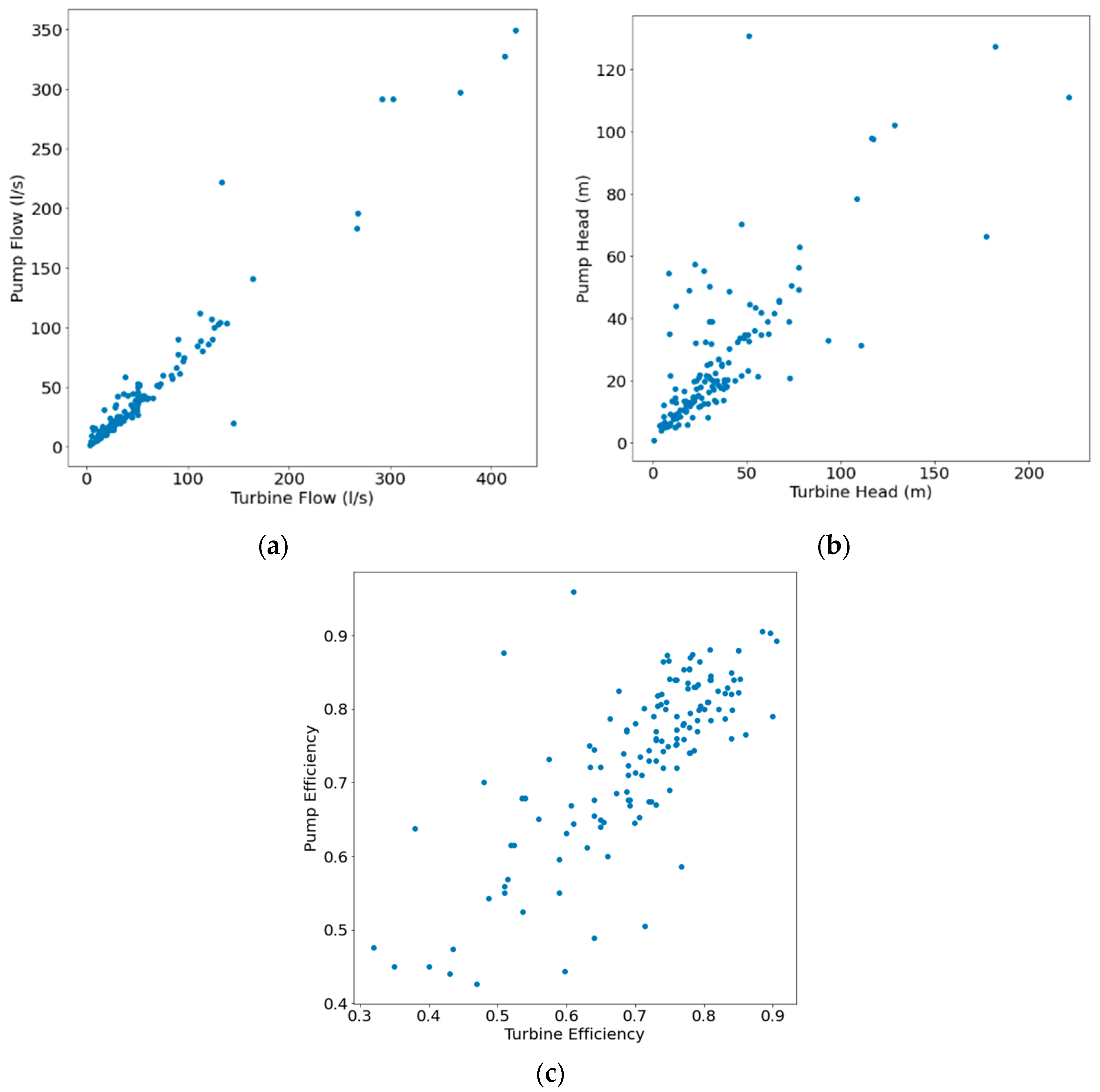
Before developing the proposed models, the target BEP turbine variables were plotted against their corresponding pump model variables. The relations between turbine and pump flow, head and efficiency are presented in Figure 2. All plots show a linear trend with the strongest being the flows and the weakest being the efficiency. It should also be noted that most of the flow rates range from 0 to 150 L/s, and a similar density trend in the head ranges from 0 to 90 m. As these datapoints fit within the typical and expected ranges of a PaT, the information beyond the maximum range is sparse and more sporadic in nature.

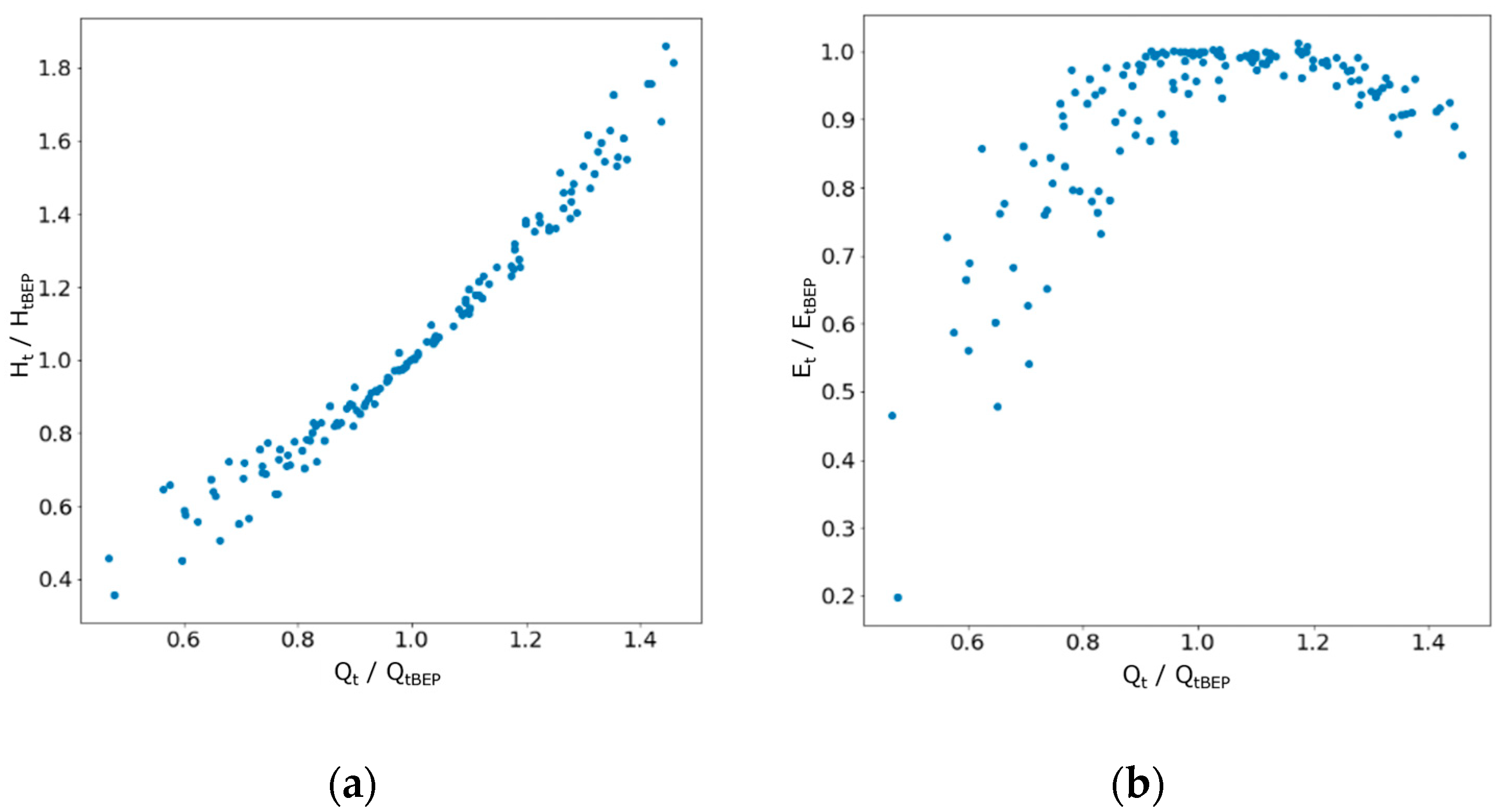
Existing characteristic curve equations, presented in Table 2, generally define the characteristics curves according to normalized head, flow and efficiency values. These normalized variables were also visualized for the current dataset, as shown in Figure 3. A near linear trend is seen in Figure 3a, with a stronger density in the mid-range and more scattering appearing on the maximum and minimums. On the other hand, Figure 3b shows a parabolic trend. Thus, a linear model may be preferred for head curves, whereas a nonlinear or polynomial linear relationship may perform best for efficiency curves.

3.1. BEP Results

The best-performing multivariate regression models for each BEP attribute based on the dimensioned and dimensionless datasets are presented in

Table 6. Multivariate Regression Results of Turbine Mode BEP Attributes with Dimensioned Datasets.

Attribute	Train/Test Split	Best Model	Default R2	Optimized R2	RMSE	MAD
Flow	80/20	Huber Regressor	0.9728	0.9721	9.7205	16.9551
Head	90/10	Elastic Net	0.9549	0.9319	7.6661	7.1337
Efficiency	80/20	Orthogonal Matching Pursuit	0.8147	0.8147	0.0505	0.0633

and

Table 7. Multivariate Regression Results of Turbine Mode BEP Attributes with Dimensionless Datasets.

Attribute	Train/Test Split	Best Model	Default R2	Optimized R2	RMSE	MAD
$\mathsf{\Phi }$	75/25	Huber Regressor	0.9749	0.9729	0.0058	0.0136
$\mathsf{\Psi }$	75/25	Huber Regressor	0.8747	0.8777	0.2227	0.0155
$\eta$	80/20	Orthogonal Matching Pursuit	0.8147	0.8024	0.0522	0.0708

, respectively. The R² scores from the default hyperparameter models are compared to the optimized models. The reduction in R² scores from the default to optimized parameters of the model is a consequence of the hyperparameter tuning and fitting the model better to the data. It should also be noted that the scales of the dimensioned parameters and the dimensionless parameters are different. Models applied to the dimensioned data set performed better than the dimensionless with regard to R². This may be explained by the fact that the dimensioned dataset contains more variables. Because dimensionless variables are normalized by impeller diameter and rotational speed, these attributes were not included separately in the dimensionless dataset.

The best BEP flow model applied the Huber Regressor and the dimensionless dataset with the following hyperparameters in scikit learn: fit intercept = False, epsilon = 1.523529, and alpha as 0.1. The Huber Regressor is a linear regression model, robust to outliers. Similarly, the best BEP head model used Elastic Net and the efficiency model, Orthogonal Matching Pursuit. These are also linear regression models, confirming the observations of Figure 2. The best BEP head model applied the following hyperparameters: selection = cyclic, positive = True, normalize = False, l1_ratio = 10, fit_intercept = False, copy_x = True, alpha = 10. And the best BEP efficiency model applied the following hyperparameters: of precompute = auto, normalize = True, fit_intercept = True, n_nonzero_coefs = 0.

The BEP predictions with ANN are overall less accurate than the multivariate regression model results, apart from the prediction of specific speeds. Dimensioned and dimensionless ANN model results are summarized in

Table 8. ANN Results of Turbine Mode BEP Attributes with Dimensioned Datasets.

Attribute	Train/Test Split	Hidden Layers	Neurons	Learning Rate	Dropout Rate	R2	RMSE	MAD
Flow	80/20	2	176	1 × 10−5	0.15437	0.914	17.068	18.256
Head	80/20	12	325	4.38 × 10−5	0.05319	0.822	11.954	13.708
Efficiency	80/20	7	310	0.00213	0	0.761	0.0573	0.0756

and

Table 9. ANN Results of Turbine Mode BEP Attributes with Dimensionless Datasets.

Attribute	Train/Test Split	Hidden Layers	Neurons	Learning Rate	Dropout Rate	R2	RMSE	MAD
$\mathsf{\Phi }$	80/20	9	124	5.5 × 10−5	0.03443	0.904	0.0126	0.012
$\mathsf{\Psi }$	80/20	6	263	0.0001005	0.4	0.885	0.0665	0.00822
$\eta$	80/20	16	207	0.000299	0	0.779	0.055	0.0607

, respectively. Similar to the multivariate regression results, the highest R² was found for flow predictions and the lowest for efficiency. However, the dimensioned dataset performed better for flow. The rectified linear unit activation function was selected through tuning for the dimensioned models, confirming the better performance of linear models.

ANNs generally require larger datasets, which are not available for the current PaT problem. Furthermore, ANN is more computationally intensive. Typically, the multivariate regression process from start to finish took around 20 min for each attribute, including training and tuning. With ANN, however, the AX optimization process took at least 25 min, up to 45 min, depending on the number of iterations required. These durations are for a laptop with a 2.1 GHz processor, in Windows 10.

Given the superiority of the multivariate regression models, their results are further explored. Figure 4 compares the models’ predicted results against actual values for all BEP attributes, for both dimensioned and dimensionless datasets. Firstly, flow results in Figure 4a,b, show the majority of predictions are close to actual values. Only one outlier is observed in both the dimensioned and dimensionless data, due to a larger PaT. This outlier is also evident in the dimensionless head predictions (Figure 4d), but not in the dimensioned head model. The dimensioned head model fits actual values well, with an R² of 0.9319, even though the majority of head values are slightly underpredicted. Efficiency results are more scattered and are identical for dimensioned (Figure 4e) and dimensionless models (Figure 4f). This is because the orthogonal matching pursuit model was applied to both. This model has no parameters which can be tuned and look for the most highly correlated attributes. In this case, the most correlated attribute to the turbine best efficiency is the pump best efficiency, which is also inherently dimensionless. Thus, choosing dimensioned or dimensionless attributes does not impact results in this case.

3.2. Characteristic Curve Results

All characteristic curve multivariate regression models performed the best with the XGB Regressor, as presented in

Table 10. Multivariate Regression Results of Turbine Mode Characteristic Curves with Dimensioned Datasets.

Curve	Train/Test Split	Model	Default R2	Optimized R2	RMSE	MAD
Head	80/20	XGB Regressor	0.993	0.997	0.0186	0.2369
Efficiency	80/20	XGB Regressor	0.908	0.901	0.0539	0.0394

and

Table 11. Multivariate Regression Results of Turbine Mode Characteristic Curves with Dimensionless Datasets.

Curve	Train/Test Split	Model	Default R2	Optimized R2	RMSE	MAD
$\mathsf{\Psi }$	80/20	XGB Regressor	0.994	0.997	0.0179	0.1940
$\eta$	80/20	XGB Regressor	0.919	0.897	0.0516	0.0364

. The results also show very similar performances for both dimensioned and dimensionless datasets. The dimensionless dataset models perform better by a small margin when considering the R² of the efficiency curves. For both datasets, the head curve was predicted with very high accuracy, with the same R² of 0.997. Hyperparameters for the best XGB Regressor models are summarized in

Table 12. Hyperparameters for best XGB Regressor models selected to predict head and efficiency curve.

Hyperparameter	Head Curve	Efficiency Curve
Subsample	0.4	0.8
n_estimators	2500	1300
Min_child_weight	1	1
Max_depth	4	9
Max_delta_step	10	6
Learning_rate	0.15	0.75
eta	0.8	0

.

The ANN results for predicting characteristics curves with the dimensioned and dimensionless datasets are summarized in

Table 13. ANN Prediction Results of Turbine Mode Characteristic Curves with Dimensioned Datasets.

Curve	Train/Test Split	Hidden Layers	Neurons	Learning Rate	Dropout Rate	R2	RMSE	MAD
Head	80/20	7	145	3.86 × 10−5	0.005	0.986	0.03848	0.20587
Efficiency	80/20	15	180	5.34 × 10−6	0	0.766	0.0776	0.0339

and

Table 14. ANN Prediction Results of Turbine Mode Characteristic Curves with Dimensionless Datasets.

Curve	Train/Test Split	Hidden Layers	Neurons	Learning Rate	Dropout Rate	R2	RMSE	MAD
$\mathsf{\Psi }$	80/20	8	141	7.27 × 10−5	0	0.980	0.0455	0.2159
$\eta$	80/20	19	100	5.73 × 10−6	0	0.816	0.0687	0.0299

, respectively. The dropout rates are consistently very small or null. Because the models rely on small datasets, lower dropouts are preferred to ensure more information can be distributed and used in training a more accurate model. The R² scores for the head and Ψ curves are high, 0.986 and 0.954 respectively, albeit lower than the multivariate regression models. The efficiency and η model scores are lower but nevertheless strong for both the dimensioned and dimensionless predictions. Still, the multivariate regression models performed better in predicting efficiency and η curve, as well. With more datapoints and possibly more attributes, the ANN may perform better. More research would be required to collect more data on PaTs. Nevertheless, the accuracy of the multivariate regression models is already high.

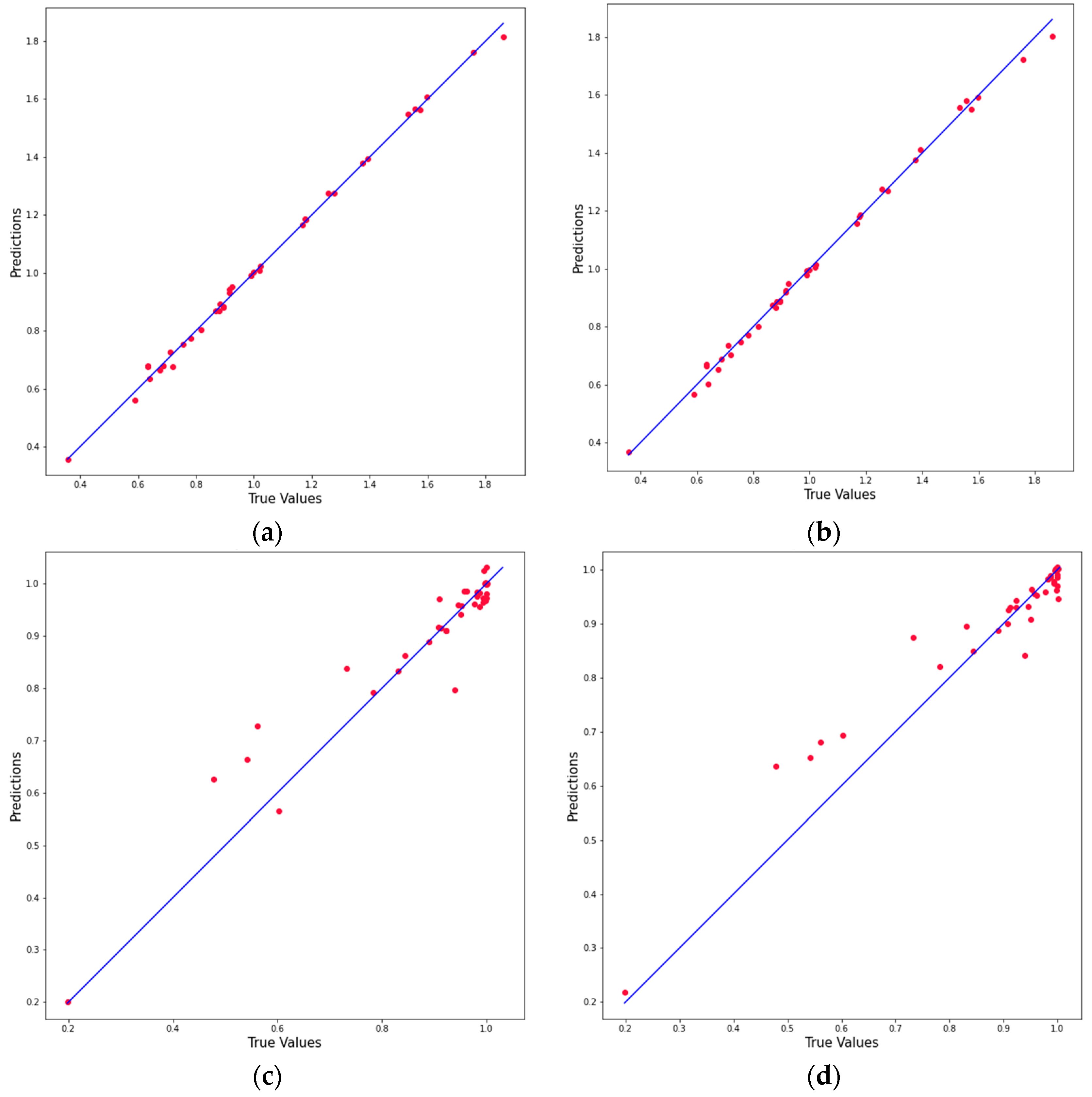
Given the superiority of the multivariate regression models, the relation between their predicted and actual results is explored in Figure 5. A very strong correlation between actual and predicted head curves is observed for all ranges of normalized head values, as shown in Figure 5a,b. Efficiency curve results are more scattered, being better fit when normalized values are closer to 1, i.e., turbine efficiency is close to the BEP. For efficiencies between 50 and 80% of the BEP, the models generally overestimate efficiency. There are also less data in this range. Thus, these models may be improved by adding more data regarding PaT performance at lower efficiencies.

4. Discussion

The performance of the models developed in the present study was also compared to those from previous research. For the BEP prediction comparison, 20 random data points were extracted from the dimensioned datasets to ensure a consistent test set. The models developed herein had different train/test splits and were thus initially tested on datasets of different sizes.

Table 15. Comparison of BEP model results.

Method	R2 Head	RMSE Head	R2 Flow	RMSE Flow
Current study multivariate regression	0.932	7.666	0.972	9.720
Current study ANN	0.822	11.954	0.914	17.068
Stepanoff [20]	0.798	8.833	0.915	16.163
Sharma [21]	0.827	13.582	0.927	17.904
Alatorre-Frenk et al. [22]	0.750	16.359	0.819	17.052
Yang at al. [9]	0.744	15.738	0.965	19.946
Barbarelli et al. [23]	−6.807	32.252	0.739	23.387
Audisio [24]	−4.97	68.161	0.971	10.685
Fontanella et al. [25]	0.391	48.772	0.967	11.34

shows the current multivariate regression models outperformed all previous models. The current head BEP multivariate regression model has an R² of 0.932, followed by the model proposed by Sharma [21] with a score of 0.827. While the ANN model performed well, with a score of 0.822, the multivariate regression model and Sharma’s equation still performed better. Other previous equations had slightly lower scores, but generally above 0.7. The exception is Barbarelli et al. [23] who developed their equations based on 4 PaTs with specific speeds ranging between 14 and 45. In the present dataset, most specific speeds were below 10. Thus, the Barbarelli et al. [23] equation is not applicable to this lower range.

The current flow BEP model has an even higher R², of 0.972. The next best-performing model is the Yang et al. [9] equation, at an R² of 0.965. The ANN model scored well, but the current multivariate regression model, Yang et al. [9], Sharma [21] and Stepanoff [20] was better. Efficiency results were not compared with previous studies because most authors did not develop a separate equation for efficiency. The PAT efficiency is not required to determine its BEP or create characteristic curves.

A comparison between the characteristic curves developed herein and other studies is provided in

Table 16. Comparison of characteristic curve model results.

Method	R2 Head Curve	RMSE Head Curve	R2 Efficiency Curve	RMSE Efficiency Curve
Current study multivariate regression	0.997	0.019	0.909	0.054
Current study ANN	0.986	0.038	0.766	0.078
Derakhshan and Nourbakhsh [26]	0.545	0.239	0.297	0.158
Rossi et al. [27]	0.983	0.047	0.777	0.089
Perez-Sanchez et al. [28]	0.955	0.076	0.868	0.068
Fontanella et al. [25]	0.874	0.126	0.869	0.068

. Again, the current multivariate regression models outperformed all previous models. The multivariate regression head curve prediction had a very high R² of 0.997, relatively higher than the Perez-Sanchez et al. [28] equation, with a value of 0.983. The ANN model scored very high as well, 0.986, which makes it the second best. The RMSE values confirm these results. The multivariate regression efficiency curve also had a high R² of 0.909, above the Rossi et al. [27] score of 0.869. In this case, the current ANN had the lowest score of the compared efficiency models. The results of the predicted efficiency curve values also scored highly using the multivariate regression method with a coefficient of determination of 0.901 with Rossi et al. [27] as the runner-up with a score of 0.869. The ANN method had a good score of 0.766 but the multivariate regression model and the Rossi et al. [27] model both performed better. Because some of these scores are very similar, the models are comparable, and their applicability might depend more on the range of pump values.

With all the scores considered, the current model is superior to that of the equations from the literature. Some of the models from the literature either scored highly in the prediction of the head curve or the efficiency curve but hardly ever at the same time. The highest scoring model for both variables would be proposed by Perez-Sanchez et al. [28] with scores of 0.955 and 0.868 for the head and efficiency curve, respectively, compared against 0.997 and 0.909 for the proposed model respectively. As for the ANN model commissioned by Rossi et al. [31], fully recreating the results and model was not possible as only information on the number of hidden layers and neurons per layer was given. Information regarding the learning rate, dropout rate, activation function, etc., was unknown. Furthermore, the training and test data sizes were unclear. Assuming that the datasets are comparable, the current model is superior in predicting the head curve variables, while Rossi et al.’s [31] model is superior in the prediction of efficiency.

The higher performance of the proposed BEP models compared to previous studies can be largely explained by the amount of data compiled. Whereas previous BEP prediction studies had datasets ranging from 4 to 32 PaTs, the present study compiled data from 145 PaTs. The comparison of multiple regression algorithms also enables the selection of the specific best-performing models for each attribute, whether BEP or characteristic curves.

Overall, the results show that linear regression models (i.e., Huber regressor, elastic net, and orthogonal matching pursuit) were specifically preferred for predicting BEP, and XGB regressors were best for predicting characteristic curves. Such models can be quickly applied in practice, facilitating the selection of PaTs in real water distribution networks. Furthermore, as data-driven multivariate regression models, they can easily be updated and improved as more data becomes available.

It is also important to highlight herein some of the worst-performing models overall considering the initial library contained a total of 24 models. Reducing the number of possibilities for the regressions can aid with future studies when considering and evaluating multiple machine learning regression models. Models that should not be considered globally for any prediction pertaining to PaTs are the Gamma Regressor, Poisson, Gamma, Inverse Gaussian, and SVR-lin. All these models showed negative R² scores, and therefore, show no promise in predicting the attributes.

Limitations

It should be noted that the comparison of the current model against other models in the literature is slightly biased. The datasets used in training each model differed. Evaluating the fit of the model to the type and range of data for which it was originally trained and tested would lead to better results. For example, Rossi et al. [33] reported higher results in their study, i.e., R² of 0.98429 for the head curve, compared to 0.955 reported herein. These scores are still lower than those of the current multivariate regression model, i.e., 0.997. Furthermore, the Rossi et al. [33] scores refer to the overall training, validation and testing dataset, whereas the results presented herein are specifically for the 20 randomly selected data points.

The current models are also limited in their application to ESOB pumps. Data were compiled specifically for this pump typology since it is the most common for PaTs. Nevertheless, multivariate regression models can be easily generalized with additional data, as opposed to earlier models that relied solely on pump efficiency and specific speed.

5. Conclusions

The present study developed novel multivariate regression models to predict PaT behavior. A dataset larger than previous studies, with 145 BEP data points, was compiled from previous work. While previous studies either applied dimensioned or dimensionless datasets, both approaches are compared herein. The developed models outperformed all previous statistical and ANN models. Results show linear regression models are specifically preferred for predicting BEP values given the underlying linear relation between pump and turbine values. The resulting R² for flow and head BEP were 0.972 and 0.932, respectively. On the other hand, the best characteristic curve predictions were developed with XGB Regressors, with R² of 0.994 and 0.919 for head and efficiency, respectively. Furthermore, the dimensionless dataset produced better characteristic curve and flow BEP models, whereas the dimensioned dataset provided slightly higher scores for head BEP models. Thus, a dimensionless dataset overall would be preferred.

The high accuracy of the developed multivariate regression models, combined with their lower computational cost compared to ANN, make them a robust solution for selecting PaTs in practice. Future studies can explore the development of broader models. Adding information for PaTs with higher flow rates or other typologies besides centrifugal ESOB, such as multistage, axial and double suction would be valuable in expanding the applicability of the models. Furthermore, the current efficiency curve models can be improved by adding datapoints to the dataset. The current dataset has between 7 and 12 datapoints per PaT. Thus, increasing the number of points per PaT could increase the accuracy of these models.

References

1. International Energy Agency. Water Energy Nexus- Excerpt from the World Energy Outlook 2016; International Energy Agency: Paris, France, 2016; p. 60. [Google Scholar]
2. McNabola, A.; Coughlan, P.; Corcoran, L.; Power, C.; Williams, A.P.; Harris, I.; Gallagher, J.; Styles, D. Energy recovery in the water industry using micro-hydropower: An opportunity to improve sustainability. Water Policy 2014, 16, 168–183. [Google Scholar] [CrossRef]
3. Stefanizzi, M.; Capurso, T.; Balacco, G.; Binetti, M.; Camporeale, S.M.; Torresi, M. Selection, control and techno-economic feasibility of Pumps as Turbines in Water Distribution Networks. Renew. Energy 2020, 162, 1292–1306. [Google Scholar] [CrossRef]
4. Mitrovic, D.; Chacón, M.C.; García, A.M.; Morillo, J.G.; Diaz, J.A.R.; Ramos, H.M.; Adeyeye, K.; Carravetta, A.; McNabola, A. Multi-country scale assessment of available energy recovery potential using micro-hydropower in drinking, pressurised irrigation and wastewater networks, covering part of the EU. Water 2021, 13, 899. [Google Scholar] [CrossRef]
5. Pérez-Sánchez, M.; Sánchez-Romero, F.J.; Ramos, H.M.; López-Jiménez, P.A. Energy recovery in existing water networks: Towards greater sustainability. Water 2017, 9, 97. [Google Scholar] [CrossRef]
6. Pugliese, F.; Giugni, M. An Operative Framework for the Optimal Selection of Centrifugal Pumps As Turbines (PATs) in Water Distribution Networks (WDNs). Water 2022, 14, 1785. [Google Scholar] [CrossRef]
7. Algieri, A.; Zema, D.A.; Nicotra, A.; Zimbone, S.M. Potential energy exploitation in collective irrigation systems using pumps as turbines: A case study in Calabria (Southern Italy). J. Clean. Prod. 2020, 257, 120538. [Google Scholar] [CrossRef]
8. Morabito, A.; Hendrick, P. Pump as turbine applied to micro energy storage and smart water grids: A case study. Appl. Energy 2019, 241, 567–579. [Google Scholar] [CrossRef]
9. Yang, S.-S.; Derakhshan, S.; Kong, F.-Y. Theoretical, numerical and experimental prediction of pump as turbine performance. Renew. Energy 2012, 48, 507–513. [Google Scholar] [CrossRef]
10. Fecarotta, O.; Carravetta, A.; Ramos, H.M. CFD and comparisons for a pump as turbine: Mesh reliability and performance concerns. Int. J. Energy Environ. 2011, 2, 39–48. [Google Scholar]
11. Ramos, H.M.; Coronado-Hernández, O.E.; Morgado, P.A.; Simão, M. Mathematic Modelling of a Reversible Hydropower System: Dynamic Effects in Turbine Mode. Water 2023, 15, 2034. [Google Scholar] [CrossRef]
12. Hongyu, G.; Wei, J.; Yuchuan, W.; Hui, T.; Ting, L.; Diyi, C. Numerical simulation and experimental investigation on the influence of the clocking effect on the hydraulic performance of the centrifugal pump as turbine. Renew. Energy 2021, 168, 21–30. [Google Scholar] [CrossRef]
13. Shojaeefard, M.H.; Saremian, S. Effects of impeller geometry modification on performance of pump as turbine in the urban water distribution network. Energy 2022, 255, 124550. [Google Scholar] [CrossRef]
14. Plua, F.; Hidalgo, V.; López-Jiménez, P.A.; Pérez-Sánchez, M. Analysis of applicability of cfd numerical studies applied to problem when pump working as turbine. Water 2021, 13, 2134. [Google Scholar] [CrossRef]
15. Shang, L.; Cao, J.; Jia, X.; Yang, S.; Li, S.; Wang, L.; Wang, Z.; Liu, X. Effect of Rotational Speed on Pressure Pulsation Characteristics of Variable-Speed Pump Turbine Unit in Turbine Mode. Water 2023, 15, 609. [Google Scholar] [CrossRef]
16. Huang, S.; Qiu, G.; Su, X.; Chen, J.; Zou, W. Performance prediction of a centrifugal pump as turbine using rotor-volute matching principle. Renew. Energy 2017, 108, 64–71. [Google Scholar] [CrossRef]
17. Marini, G.; Di Menna, F.; Maio, M.; Fontana, N. Selection for Microhydropower Generation and Pressure Regulation in a Water Distribution Network (WDN). Water 2023, 15, 2807. [Google Scholar] [CrossRef]
18. Rossi, M.; Fanti, O.; Pacca, S.A.; Comodi, G. Energy efficiency intervention in urea processes by recovering the excess pressure through hydraulic power recovery Turbines (HPRTs). Sustain. Energy Technol. Assess. 2022, 52, 102263. [Google Scholar] [CrossRef]
19. Esmaeilian, H.R.; Fadaeinedjad, R.; Bakhshai, A. Performance Evaluation and MPPT Control of a Variable-Speed Pump-as-Turbine System. IEEE Syst. J. 2023, 17, 3117–3126. [Google Scholar] [CrossRef]
20. Stepanoff, A.J. Centrifugal and Axial Flow Pumps: Theory, Design and Application; John Wiley: New York, NY, USA, 1957. [Google Scholar]
21. Sharma, K.R. Small Hydroelectric Project-Use of Centrifugal Pumps as Turbines; Kirloskar Electric Co.: Bangalore, India, 1985. [Google Scholar]
22. Alatorre-Frenk, C.; Ml, A.; Karin, A. Cost Minimisation in Micro-Hydro Systems Using Pumps-as-Turbines. Ph.D. Thesis, University of Warwick, Coventry, UK, 1994. [Google Scholar]
23. Barbarelli, S.; Amelio, M.; Florio, G. Experimental activity at test rig validating correlations to select pumps running as turbines in microhydro plants. Energy Convers. Manag. 2017, 149, 781–797. [Google Scholar] [CrossRef]
24. Audisio, O. Bombas Utilizadas Como Turbinas; Universidad Nacional del Comahue: Buenos Aires, Argentina, 2009. [Google Scholar]
25. Fontanella, S.; Fecarotta, O.; Molino, B.; Cozzolino, L.; Della Morte, R. A performance prediction model for pumps as turbines (PATs). Water 2020, 12, 1175. [Google Scholar] [CrossRef]
26. Derakhshan, S.; Nourbakhsh, A. Experimental study of characteristic curves of centrifugal pumps working as turbines in different specific speeds. Exp. Therm. Fluid Sci. 2008, 32, 800–807. [Google Scholar] [CrossRef]
27. Rossi, M.; Nigro, A.; Renzi, M. Experimental and numerical assessment of a methodology for performance prediction of Pumps-as-Turbines (PaTs)operating in off-design conditions. Appl. Energy 2019, 248, 555–566. [Google Scholar] [CrossRef]
28. Pérez-Sánchez, M.; Sánchez-Romero, F.J.; Ramos, H.M.; López-Jiménez, P.A. Improved planning of energy recovery in water systems using a new analytic approach to PAT performance curves. Water 2020, 12, 468. [Google Scholar] [CrossRef]
29. Niu, X.; Yang, C.; Wang, H.; Wang, Y. Investigation of ANN and SVM based on limited samples for performance and emissions prediction of a CRDI-assisted marine diesel engine. Appl. Therm. Eng. 2017, 111, 1353–1364. [Google Scholar] [CrossRef]
30. Rodríguez, J.; Hamzaoui, Y.; Hernández, J.; García, J.; Flores, J.; Tejeda, A. The use of artificial neural network (ANN) for modeling the useful life of the failure assessment in blades of steam turbines. Eng. Fail. Anal. 2013, 35, 562–575. [Google Scholar] [CrossRef]
31. Rossi, M.; Renzi, M. A general methodology for performance prediction of pumps-as-turbines using Artificial Neural Networks. Renew. Energy 2018, 128, 265–274. [Google Scholar] [CrossRef]
32. Telikani, A.; Rossi, M.; Khajehali, N.; Renzi, M. Pumps-as-Turbines’ (PaTs) performance prediction improvement using evolutionary artificial neural networks. Appl. Energy 2023, 330, 120316. [Google Scholar] [CrossRef]
33. Balacco, G. Performance prediction of a pump as turbine: Sensitivity analysis based on artificial neural networks and evolutionary polynomial regression. Energies 2018, 11, 3497. [Google Scholar] [CrossRef]
34. Fecarotta, O. RPS: REDAWN PAT Selection App. 2021. Available online: https://zenodo.org/record/4973447 (accessed on 28 August 2021).
35. Tan, X.; Engeda, A. Performance of centrifugal pumps running in reverse as turbine: Part Ⅱ- systematic specific speed and specific diameter based performance prediction. Renew. Energy 2016, 99, 188–197. [Google Scholar] [CrossRef]
36. Stefanizzi, M.; Capurso, T.; Balacco, G.; Torresi, M.; Binetti, M.; Piccinni, A.F.; Fortunato, B.; Camporeale, S.M. Preliminary assessment of a pump used as turbine in a water distribution network for the recovery of throttling energy. In Proceedings of the 13th European Turbomachinery Conference on Turbomachinery Fluid Dynamics and Thermodynamics, ETC 2019, Lausanne, Switzerland, 8–12 April 2019. [Google Scholar] [CrossRef]
37. Rawal, S.; Kshirsagar, J.T. Numerical Simulation on a Pump Operating in a Turbine Mode. In Proceedings of the 23rd International Pump Users Symposium, Houston, TX, USA, 5–8 March 2007; pp. 21–28. [Google Scholar]
38. Su, X.; Huang, S.; Li, Y.; Zhu, Z.; Li, Z. Numerical and experimental research on multi-stage pump as turbine system. Int. J. Green Energy 2017, 14, 996–1004. [Google Scholar] [CrossRef]
39. Polák, M. Experimental evaluation of hydraulic design modifications of radial centrifugal pumps. Agron. Res. 2017, 15, 1189–1197. [Google Scholar]
40. Nygren, L. Hydraulic Energy Harvesting with Variable Speed Driven Centrifugal Pump as Turbine. Pap. Knowl. Towar. A Media Hist. Doc. 2014, 5, 40–51. [Google Scholar]
41. Yousefi, H.; Noorollahi, Y.; Tahani, M.; Fahimi, R. Modification of pump as turbine as a soft pressure reduction systems (SPRS) for utilization in municipal water network. Energy Equip. Syst. 2019, 7, 41–56. [Google Scholar]
42. Giosio, D.; Henderson, A.; Walker, J.; Brandner, P.; Sargison, J.; Gautam, P. Design and performance evaluation of a pump-as-turbine micro-hydro test facility with incorporated inlet flow control. Renew. Energy 2015, 78, 1–6. [Google Scholar] [CrossRef]
43. Yang, S.-S.; Kong, F.-Y.; Chen, H.; Su, X.-H. Effects of blade wrap angle influencing a pump as turbine. J. Fluids Eng. Trans. ASME 2012, 134, 061102. [Google Scholar] [CrossRef]
44. Abazariyan, S.; Rafee, R.; Derakhshan, S. Experimental study of viscosity effects on a pump as turbine performance. Renew. Energy 2018, 127, 539–547. [Google Scholar] [CrossRef]
45. Moussaoui, M.; García, J.P. Estudio Sobre Bombas Funcionando Como Turbinas (BFT). Selección, Montaje y Caracterización Experimental de un Prototipo Para Banco de Ensayos Docente; Universidad Politécnica de Cartagena: Cartagena, Spain, 2017. [Google Scholar]
46. Frosina, E.; Buono, D.; Senatore, A. A Performance Prediction Method for Pumps as Turbines (PAT) Using a Computational Fluid Dynamics (CFD) Modeling Approach. Energies 2017, 10, 103. [Google Scholar] [CrossRef]
47. Albert, Ø. Pump as Turbine-Symmetry Prediction Method for Pump as Turbine Characteristics. Master’s Thesis, NTNU, Trondheim, Norway, 2018. [Google Scholar]
48. Fernández, J.; Barrio, R.; Blanco, E.; Parrondo, J.L.; Marcos, A. Numerical investigation of a centrifugal pump running in reverse mode. Proc. Inst. Mech. Eng. Part A J. Power Energy 2010, 224, 373–381. [Google Scholar] [CrossRef]
49. Sedlár, M.; Soukal, J.; Komárek, M. CFD Analysis of Middle Stage of Multistage Pump Operating in Turbine Regime. Eng. Mech. 2009, 16, 413–421. [Google Scholar]
50. Delgado, J.; Ferreira, J.; Covas, D.; Avellan, F. Variable speed operation of centrifugal pumps running as turbines. Experimental investigation. Renew. Energy 2019, 142, 437–450. [Google Scholar] [CrossRef]
51. Kramer, M.; Terheiden, K.; Wieprecht, S. Pumps as turbines for efficient energy recovery in water supply networks. Renew. Energy 2018, 122, 17–25. [Google Scholar] [CrossRef]
52. Singh, P. Optimization of Internal Hydraulics and of System Design for PUMPS as TURBINES with Field Implementation and Evaluation; Institut für Wasser und Gewässerentwicklung: Karlsruhe, Germany, 2005. [Google Scholar]
53. Jain, S.V.; Swarnkar, A.; Motwani, K.H.; Patel, R.N. Effects of impeller diameter and rotational speed on performance of pump running in turbine mode. Energy Convers. Manag. 2015, 89, 808–824. [Google Scholar] [CrossRef]
54. Bakshy, E.; Dworkin, L.; Karrer, B.; Kashin, K.; Letham, B.; Murthy, A.; Singh, S. AE: A domain-agnostic platform for adaptive experimentation. In Proceedings of the Nips, Montréal, QC, Canada, 3–8 December 2018; p. 8. [Google Scholar]
Figure 1. Flowchart of (a) multivariate regression and (b) ANN model development.
Water 15 03290 g001
Figure 2. Pump vs. Turbine BEP Values for Flow (a), Head (b), and Efficiency (c).
Water 15 03290 g002
Figure 3. Normalized Turbine Flow against Normalized Turbine Head (a) and Efficiency (b).
Water 15 03290 g003
Figure 4. Predicted vs. Actual Values for Multivariate Regression Models of (a) Flow—Dimensioned, (b) Flow—Dimensionless, (c) Head—Dimensioned, (d) Head—Dimensionless, (e) Efficiency—Dimensioned. (f) Efficiency—Dimensionless.
Water 15 03290 g004
Figure 5. Predicted vs. Actual Values for Multivariate Regression Models of (a) Head Curve—Dimensioned, (b) Head curve—Dimensionless, (c) Efficiency curve—Dimensioned, (d) Efficiency curve—Dimensionless.
Water 15 03290 g005