1. Introduction
Many countries face a scarcity of domestically produced energy, resulting in a widespread appreciation for the stable supply of green energy. Renewable energy has already become the trend of future energy developments [
1]. According to data from the Bureau of Energy, Taiwan [
2], there has been a yearly increasing trend in the amount of solar energy generated in Taiwan. In 2022, solar energy generation reached 10,677 GWh, accounting for 44.78% of the total renewable energy output. The development of Taiwan’s aquaculture industry is thriving, and the transformation of the fishery industry into an integrated fishery–electricity structure is in line with current trends. The combustion of fossil fuels, especially coal, gasoline, and diesel, is a major source of airborne particulate matter (PM) and ground-level ozone pollution, both of which are considered key factors in the global burden of mortality and disease [
3]. The integration of photovoltaic facilities with traditional aquaculture can reduce the consumption of chemical energy (fossil fuels), lower the expenditure on electricity for aquaculture, and provide a stable supply of clean energy, with potential benefits for energy and the production efficiency of aquaculture in the future [
4]. When fishponds are transformed into floating photovoltaic systems combined with aquaculture, they shade a portion of sunlight from the ponds’ surface, affecting the biological systems within. This impact includes changes in algal growth due to variations in light, which subsequently alter the nutrient factors in the water [
5]. Changes in light exposure also affect the embryonic development of aquatic organisms, leading to disturbances in the growth of fry [
6]. Apart from the embryonic stage, variations in light can influence the larval growth, color, and physiological mechanisms of fish and the ecological factors that affect the larval growth of fish. Some of these factors are light intensity, photoperiod, turbidity, predation, competition, and food availability [
7].
The main advantages of developing floating photovoltaic systems include the fact that no land resources are needed, and the systems have rapid mobility and are easy to assemble. Moreover, floating photovoltaic systems have a higher power generation efficiency than terrestrial systems [
7,
8]. Floating photovoltaic systems are typically installed on the surface of reservoirs, and their benefits are being assessed by many countries in various rivers and reservoirs [
9]. The shading effect of floating photovoltaics can reduce the evaporation of water, making them suitable for operations and applications that use solar power generation in water bodies [
10,
11]. They also demonstrate superior power-generating capabilities [
12,
13].
Litopenaeus vannamei and Chanos chanos are species extensively cultivated in Southern Taiwan. L. vannamei, introduced to Taiwan by the Fisheries Agency of the Council of Agriculture in the early 1980s, is a euryhaline tropical shrimp species. It can thrive in salinities ranging from 0 to 35‰ and tolerates a temperature range of 15–38 °C, with an optimal growth temperature of 22–35 °C. It is confined to regions where the water temperatures remain above 20 °C (68 °F) throughout the year, establishing itself as one of the four major cultivated shrimp species in Taiwan. C. chanos is one of the primary aquaculture species in Taiwan and is native to tropical and subtropical waters. This species can adapt to a variety of salinity conditions, from freshwater in rivers to brackish waters in estuarine mangrove areas, lagoons, and marine environments, such as sandy terrains or coral reefs. Artificial breeding of this species has also been successfully achieved. However, C. chanos is less tolerant of cold. Its resistance diminishes below 14 °C, and there are occurrences of mortality when temperatures drop below 10 °C. Therefore, preparations for overwintering are necessary during its cultivation. According to Taiwan’s cumulative table of stocked fish species, there are currently 1686 households cultivating L. vannamei, spanning an area of 963 hectares, with 3855 fishponds stocked. As per Taiwan’s Fisheries Yearbook 2018, the area dedicated to the cultivation of C. chanos in Taiwan is 9721 hectares, of which 5838 hectares are saltwater fishponds and 3883 hectares are freshwater fishponds, according to the Fisheries Agency of the Council of Agriculture. The co-cultivation of C. chanos and L. vannamei is prevalent in Southern Taiwan, highlighting the potential importance of a model combining the co-cultivation of C. chanos plus L. vannamei and photovoltaic aquaculture in the fisheries industry.
Coastal fishponds are vulnerable to the impact of seasonal fluctuations in rainfall and temperature, which can lead to drastic changes in a pond’s salinity. Such changes can cause significant fluctuations in the concentrations of nitrates, nitrites, and ammonium in the water, affecting the growth, physiological functions, and survival of aquatic organisms. Nitrites and ammonium, in particular, can affect the physiological regulation and survival of aquatic organisms [
14,
15]. Monitoring the pH levels in aquaculture ponds can be used to determine the concentration of inorganic acids in the water [
16]. Measuring the oxidation–reduction potential (ORP) of the water in aquaculture ponds can serve as an indicator for assessing the water’s oxidizing and reducing abilities [
17] and thereby evaluating the concentration of organic matter. The conductivity of the water can be used as an index for monitoring water quality and the concentration of metallic salts. Through these indicators, we can analyze changes in water quality in the symbiotic fishery–solar power model, and the basic information of the cultured organisms can be used to modify the conditions for aquacultural management.
The effects of combining floating solar facilities with the co-cultivation of C. chanos and L. vannamei on aquaculture have not been extensively explored. This study underscores the importance of concurrently evaluating various parameters of water quality and cultivation in the cultivation of mixed species, particularly under varying rates of solar shading. This study used solar panels with shading rates of 40% and 0% to investigate their impact on traditional cultivation parameters, such as biological growth, temperature, salinity, pH, dissolved oxygen, redox potential, conductivity, nitrates, nitrites, and ammonium. The goal was to clarify the status of these parameters when applied to the symbiotic fishery–solar power model, which will potentially benefit the innovation and transformation of the aquaculture industry in the future. This study’s main contribution is that it evaluated the effects of solar shading on water quality and the growth of L. vannamei and C. chanos in a symbiotic fishery–solar power model. The study demonstrated the feasibility and advantages of combining aquaculture with the generation of photovoltaic power, which can enhance the production efficiency of L. vannamei and C. chanos, improve the water’s quality, reduce the consumption of fossil fuels, and provide stable and clean energy. This study also offers valuable insights for the innovation and transformation of aquaculture in the future and suggests its potential benefits for countries facing challenges of energy self-sufficiency.
2. Method
2.1. Study Area
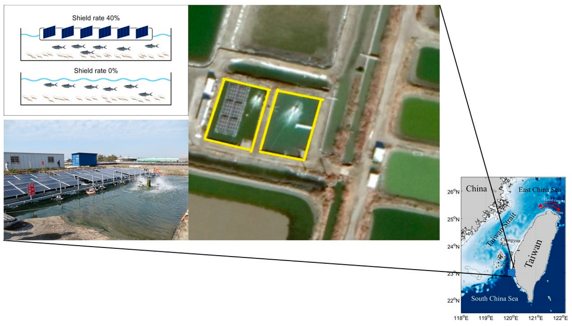
The study was conducted at a
C. chanos farm integrated with a floating solar photovoltaic facility. The farm is part of the Marine Aquaculture Research Center of the Fisheries Research Institute, Council of Agriculture, Executive Yuan (geographical coordinates: 23°0713.7″ N 120°04′49.8″ E;
Figure 1). The research took place from October 2018 to May 2019, with solar photovoltaic panels mounted on the rafts for experimentation. The experimental group’s farm covered an area of 0.03 hectares, featuring a floating platform composed of rubber and stainless steel for the solar photovoltaic system. The area shaded by the photovoltaic system constituted 40% of the pond’s total area (this part is hereafter referred to as the experimental group). For comparison, a control group with a shading rate of 0% was established.
2.2. Biological Monitoring
In Taiwan, the co-cultivation of L. vannamei and C. chanos is quite prevalent. Therefore, this study attempted to integrate photovoltaics into the co-cultivation of L. vannamei and C. chanos. The stocking density of L. vannamei was determined based on the Fisheries Yearbook of the Tainan area, with a benchmark of 400,000 to 1,000,000 individuals per hectare. Given the total farming area of 0.06 hectares in both groups, each treatment group was stocked with 25,000 black-shelled shrimp larvae. Artificial feed was provided once in the morning and once in the afternoon daily. In this study, the cultivation of L. vannamei utilized an artificial feed named “Nan Shui Yan No. 1 Prawn Feed” developed and produced by the Taiwan Fisheries Research Institute. For C. chanos, the artificial feed comprised sinking-type (PM) fish meal from Pesquera Diamante S.A. (Lima, Peru) and Austral Group S.A.A. (Lima, Peru), soybean meal from the Da Tong Yi and Zhong Lian Oil & Fats Company, and vitamins and minerals supplied by Multi-advance Biotechnology Co., Ltd. (Taoyuan City, Taiwan) The average water depth of the pond varied between 200 cm and 250 cm. During the cultivation period, changes in the water were minimal, with seawater only added when the water level was too low or the salinity was too high. Each pond was equipped with a water wheel and a water pump, with natural seawater from a lagoon being introduced into the pond. The weight and total length of the organisms were recorded monthly, with a minimum of 10 samples taken from each group. Each pond was stocked with 700 C. chanos with an initial weight of 3.18 ± 0.92 g and a body length of 7.47 ± 0.64 cm. The weight and total length were also recorded monthly, with a minimum of 10 samples taken from each group. In this study, the mortality rates of L. vannamei and C. chanos were effectively controlled to less than 5%, aligning with the mortality rate standards for aquaculture set by the Council of Agriculture in Taiwan. The experimental cultivation period spanned six months.
2.3. Pond Preparation
Typically, after harvest, the bottom of the pond is cleared, which involves the cleaning of the entire pond, sludge, and the drying area, and the application of lime for disinfection. After the pond has been drained, sunlight is utilized to dry the bottom soil, leading to comprehensive oxidation of the soil. The soil is then tilled using an excavator to expose and level the underlying layers. Lime, at a rate of 100 kg per square meter, is evenly spread across the pond. Water is then introduced to a depth of 30 cm and supplemented with sodium hypochlorite up to a concentration of 10 ppm and left to soak for three to five days for disinfection. Subsequently, 60 kg of tea seed meal per square meter is added. Aeration is carried out using a water wheel for seven days until the bubbles disappear. When microalgae and feed organisms start to grow, larvae can be introduced into the pond.
2.4. Water Quality Measurement Parameters
The salinity of the water in the aquaculture ponds was around 30–42 psu. During the experimental period, a water quality monitor was used to measure the pond water every two weeks at 09:00 and 16:00 for (i) the surface layer of the pond (0–10 cm below the surface), (ii) the middle layer of the pond (80–100 cm below the surface), and (iii) the bottom layer of the pond (0–10 cm above the pond’s bottom), for recording and analysis. The parameters we recorded and analyzed included the temperature, salinity, pH, dissolved oxygen, oxidation–reduction potential, and conductivity. These were measured using a multifunction water-quality measuring instrument, the Hydrolab Quanta, from the Woonsocket, RI, USA. Additionally, nitrites (NO2−, HANNA HI96707, Villafranca Padovana, Italy), ammonium (NH4+, HANNA HI96700, Italy), and ammonia (NH3+, HANNA HI96700, Italy) were sampled at 10:30 am using a water sampler at a depth of 30–50 cm in the pond water. The samples were placed in a 1 L sampling bottle and taken to the laboratory for analysis. To achieve a true representation of the actual experimental conditions, parameters such as the temperature, salinity, dissolved oxygen, pH, oxidation–reduction potential, and conductivity values were analyzed and compared at 09:00 and 16:00 to confirm their actual differences. Additionally, during the research process, an automatic water-quality monitoring system from the Kuan Wei Company was used to monitor and record the temperature, dissolved oxygen, pH, and oxidation–reduction potential values of the aquaculture pond’s water 24 h a day. The monitoring instruments were cleaned and maintained weekly to preserve their sensitivity.
2.5. Statistical Analysis
In the co-cultivation of L. vannamei and C. chanos integrated with floating photovoltaic power generation, an independent-sample t-test (with α set at 0.05) was used for statistical analysis by IBM SPSS 18 Statistics software. This study opted for the independent-sample t-test because it is a commonly used statistical method for comparing the means of two groups and determining whether there is a significant difference between them. The t-test was deemed to be most appropriate for our dataset and the specific comparisons we aimed to make, ensuring clarity and precision in our findings. This was used to compare the monthly factors of water quality between the experimental groups (with 40% and 0% shading) and the control group.
4. Discussion
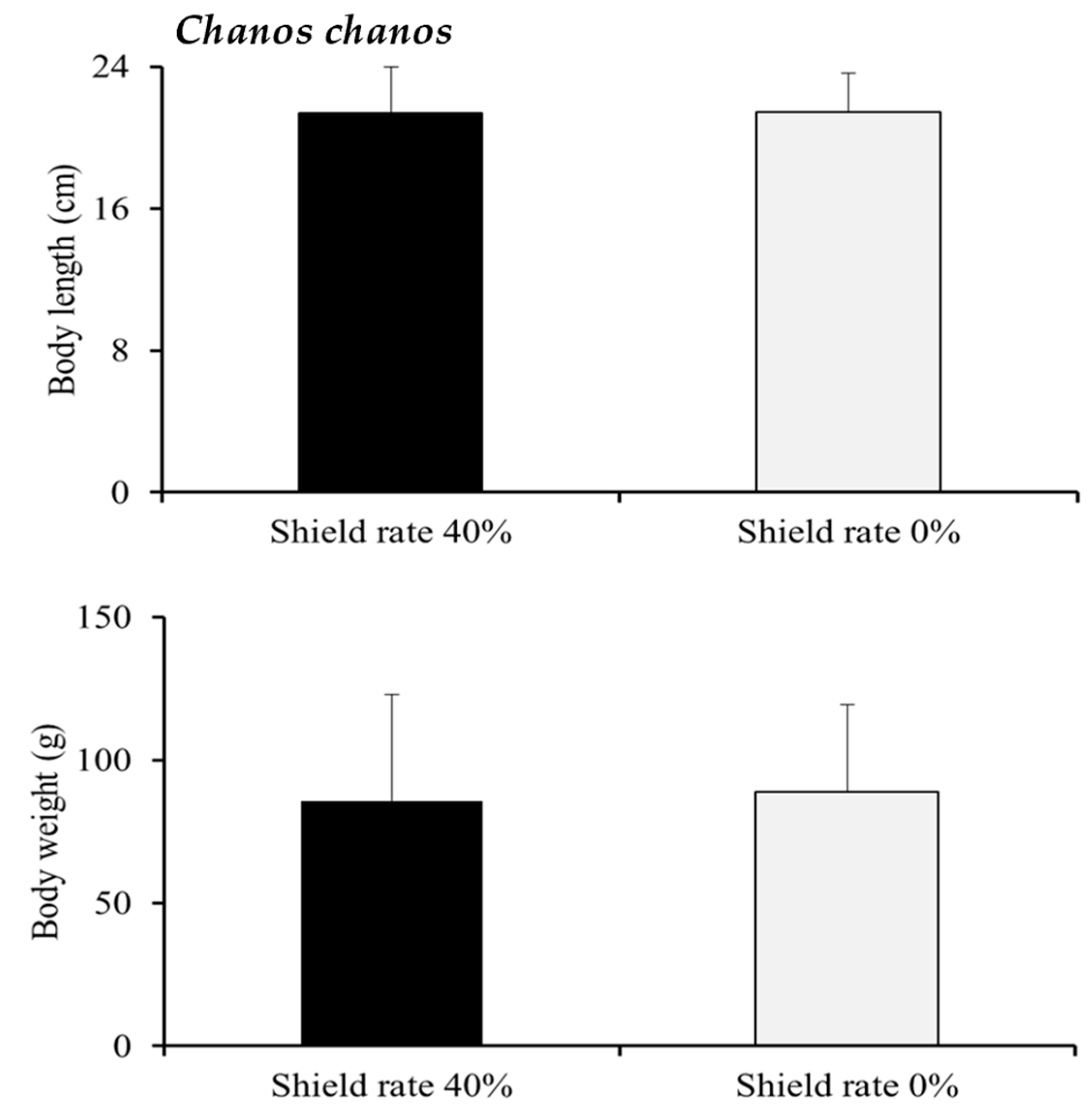
Environmental factors in bodies of water undergo significant changes in response to monthly variations in the climate. In the final phase of cultivation, specifically during spring, the feeding activity of the fish increased, which led to an increased amount of feed being supplied and a subsequent significant rise in the nitrite and ammonium levels. The
C. chanos fish grown in the 40% shading group displayed faster growth with significant differences in length and weight. In this study, our observations showed that during the early stages of stocking, juvenile
C. chanos would school and feed at the pond’s surface during the day, making them vulnerable to bird attacks around sunrise and sunset. According to the research in [
18], the economic losses caused by piscivorous birds in the process of aquaculture account for 10% of the yield. The growth of white shrimp cultured in groups with a 40% shading rate showed a quicker increase in weight and length. The floating solar photovoltaic system with a 40% shading treatment maintained lower temperatures throughout the cultivation process, which helped reduce water evaporation, improve the ecosystem, and promote the growth of fish [
19].
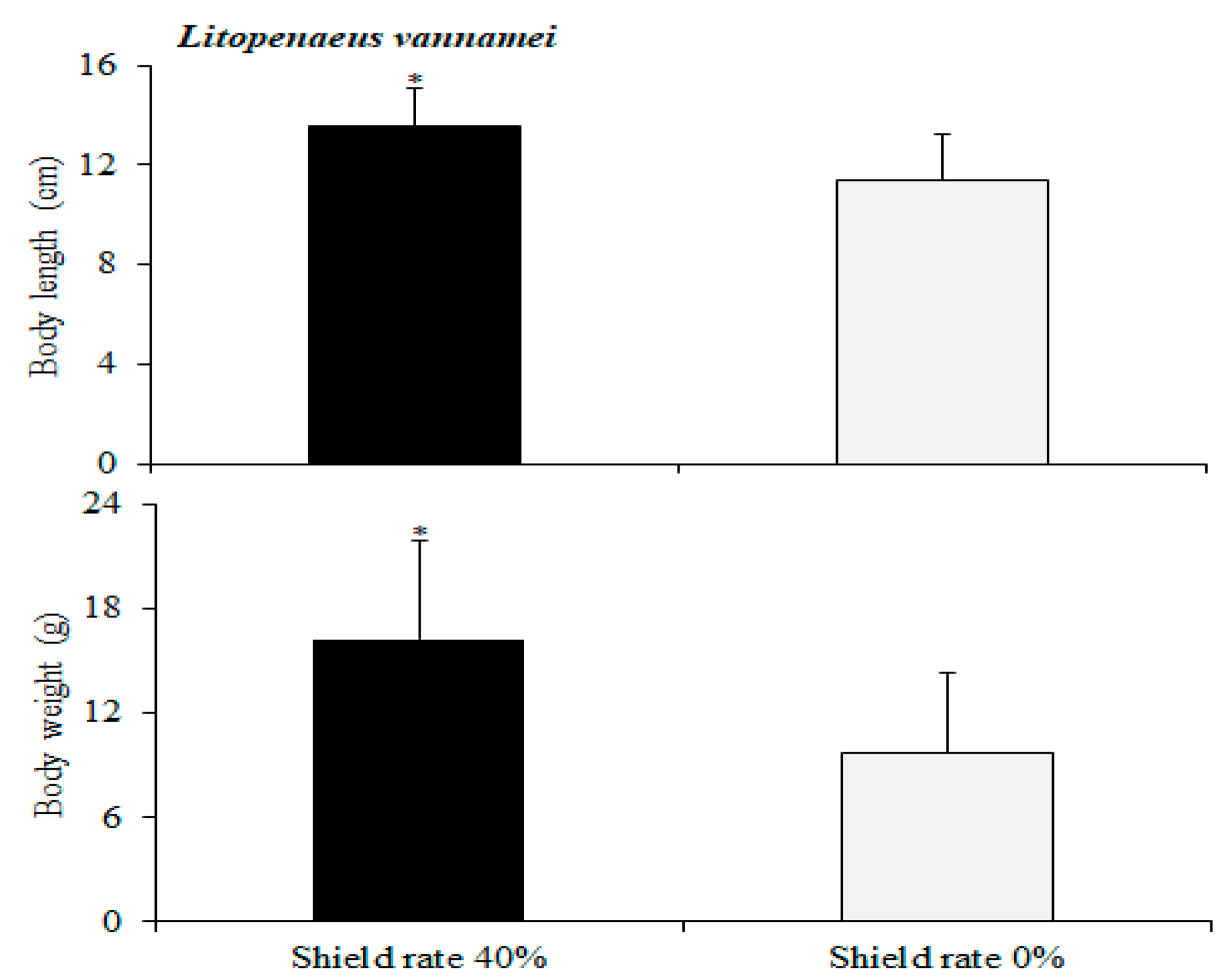
In this study, our observations revealed that the growth of
L. vannamei was faster in the group with a 40% shading rate. This is attributed to the high quantity of fine algae attached underneath the raft, providing the shrimp with a natural food source. The floating solar photovoltaic system helped to maintain a lower water temperature [
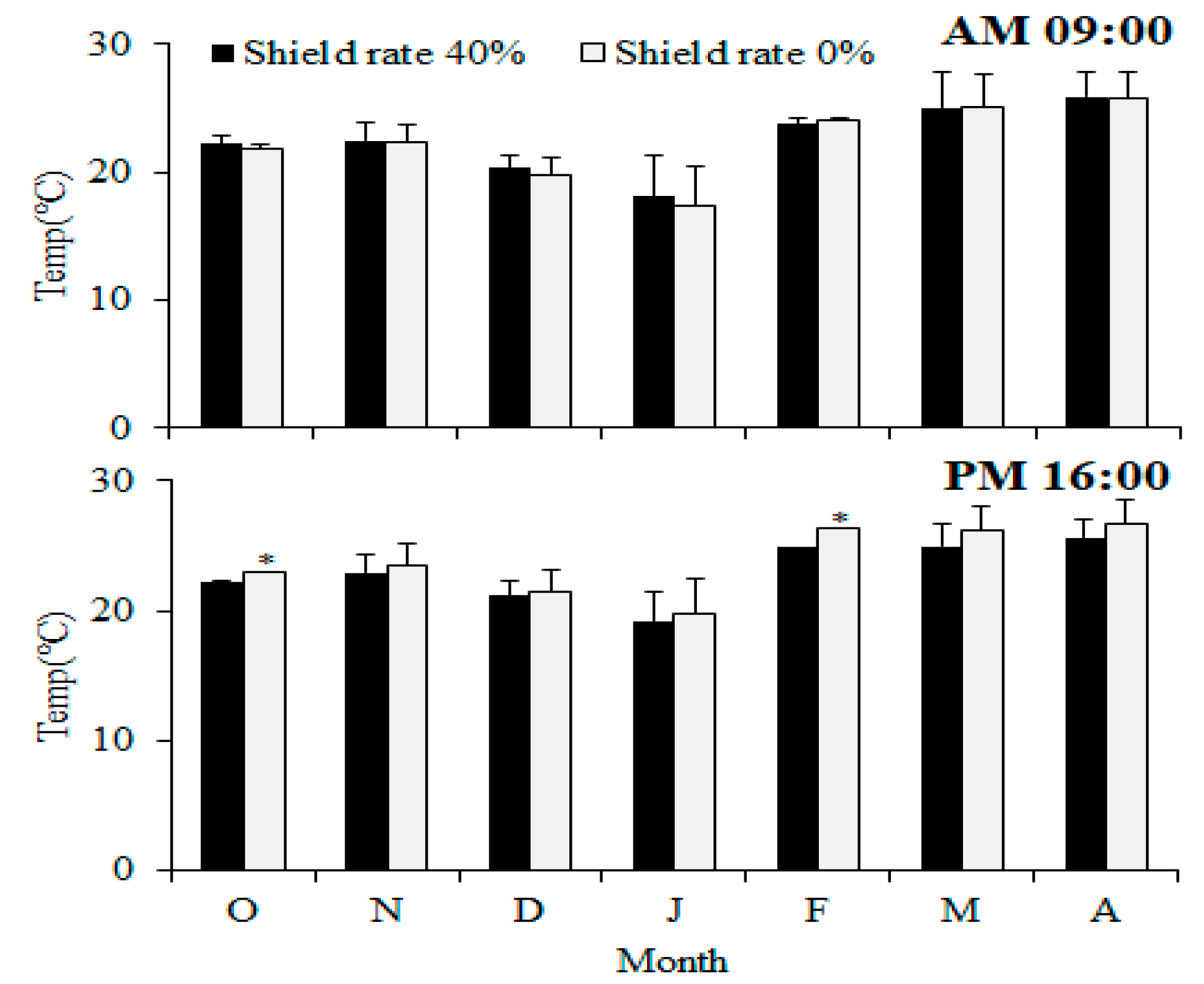
8,
9,
20]. During the experiment, temperature fluctuations were minor in the morning, while the afternoon fluctuations were more pronounced. A swift decline in salinity due to rainfall resulted in a large-scale die-off of algae in the cultivation ponds, as they could not adapt to the sudden changes. This led to larger temperature disparities between the two groups. Hence, the 40% shading treatment group demonstrated improved growth of cultivated
C. chanos, providing more stable breeding conditions. According to a study by [
21], extreme temperature variations can affect the metabolism, movement, growth, and reproduction of aquatic organisms. By implementing floating solar photovoltaic systems, the impact of extreme climate on aquaculture organisms can be reduced, thereby minimizing their energy depletion. Consequently, the group with the 40% shading rate demonstrated enhanced growth of
C. chanos in aquaculture, and the cultivation conditions were relatively stable. The 0% shading treatment group experienced larger average temperature fluctuations, leading to a collapse in the microalgal population during the changes in climate during autumn. In contrast, the 40% shading treatment group, with its smaller average temperature changes, witnessed minor changes in the concentration of algae, thus maintaining a more stable average daily temperature and reducing the risk of algal blooms. Both
L. vannamei and
C. chanos prefer warmer conditions, and the 40% shading treatment group experienced smaller fluctuations in temperature during winter. When cold fronts arrived, the ponds’ temperatures dropped more gradually, providing the aquatic organisms with more time to adapt and thereby reducing the damage caused by cold fronts. The survival of white shrimp juveniles is optimal at temperatures between 20 °C and 30 °C and at salinities above 20‰ [
22]. For prawns, the optimal temperature is approximately 27 °C [
23]. Furthermore, research has shown that the growth of juvenile fish is better in a warmer environment with sufficient food compared with cooler environments [
24]. When the 40% shading group encountered significant climate changes, there were fewer fluctuations in the temperature and algae, resulting in less physiological impact on the fish and shrimp.
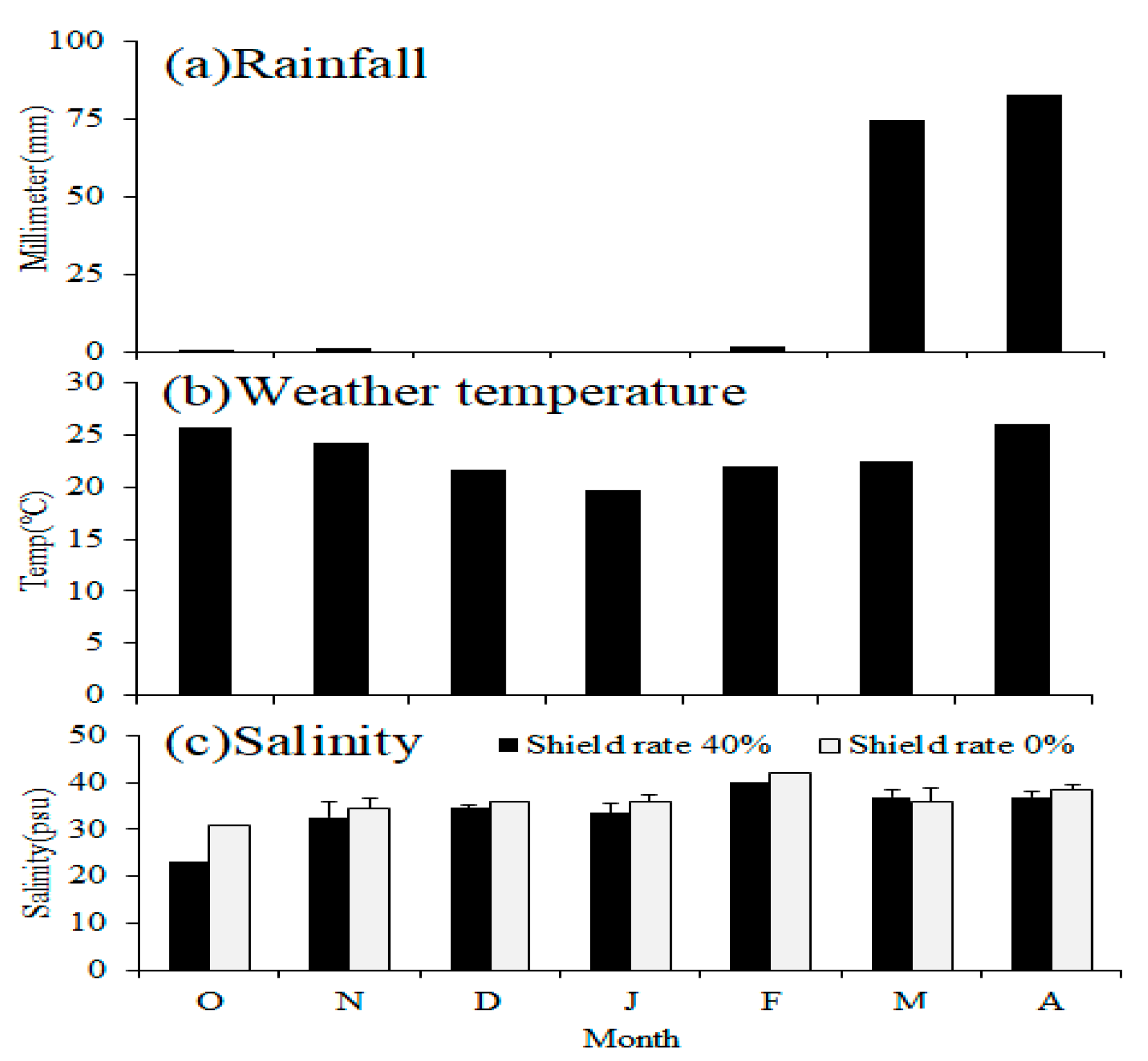
Starting in October, Tainan experiences reduced sunlight and temperature during autumn, leading to a decrease in photosynthesis in the ponds and a massive die-off of algae. Numerous studies have confirmed that the shading effect of floating solar photovoltaic facilities can decrease water evaporation [
10,
11]. As a result, this not only stabilizes the water’s quality but also conserves water resources, making it suitable for application in aquaculture models. As evidenced by the temperature and rainfall graphs from the meteorological bureau, the differences in salinity between the two treatment groups are a result of seasonal changes. The 40% shading treatment group displayed minor changes in salinity, illustrating its effectiveness in reducing water evaporation (
Figure 4). In contrast, the 0% shading treatment group experienced larger changes in salinity, heavily influenced by climatic factors, particularly during winter or cold fronts, when photosynthesis decreased and salinity rapidly surged to over 40 psu, resulting in a massive die-off of algae in the cultivation ponds. In the application of power generation models for aquaculture, this study has found that the floating photovoltaic system in brackish fishponds aids in mitigating drastic changes in salinity. This indirectly helps to preserve the functionality of the fishpond and allows the aquatic organisms to conserve energy, which would otherwise be expended to regulate osmotic pressure due to the rapid changes in salinity. According to the literature [
25,
26], both fish and crustaceans need to consume energy to maintain osmotic balance within their bodies. Slowing down the rapid changes in salinity can indirectly reduce the energy consumed by aquatic organisms for regulating osmotic pressure. As a result,
L. vannamei in the group with 40% shading grew faster. However, precautions need to be taken to prevent the invasion of exotic species, such as tilapia, flower frogs, and crabs. Pre-treatment of the pond water through, for example, disinfection with chlorine tablets can lessen the chance of invasion by foreign organisms and block the path of natural enemies and pathogens.
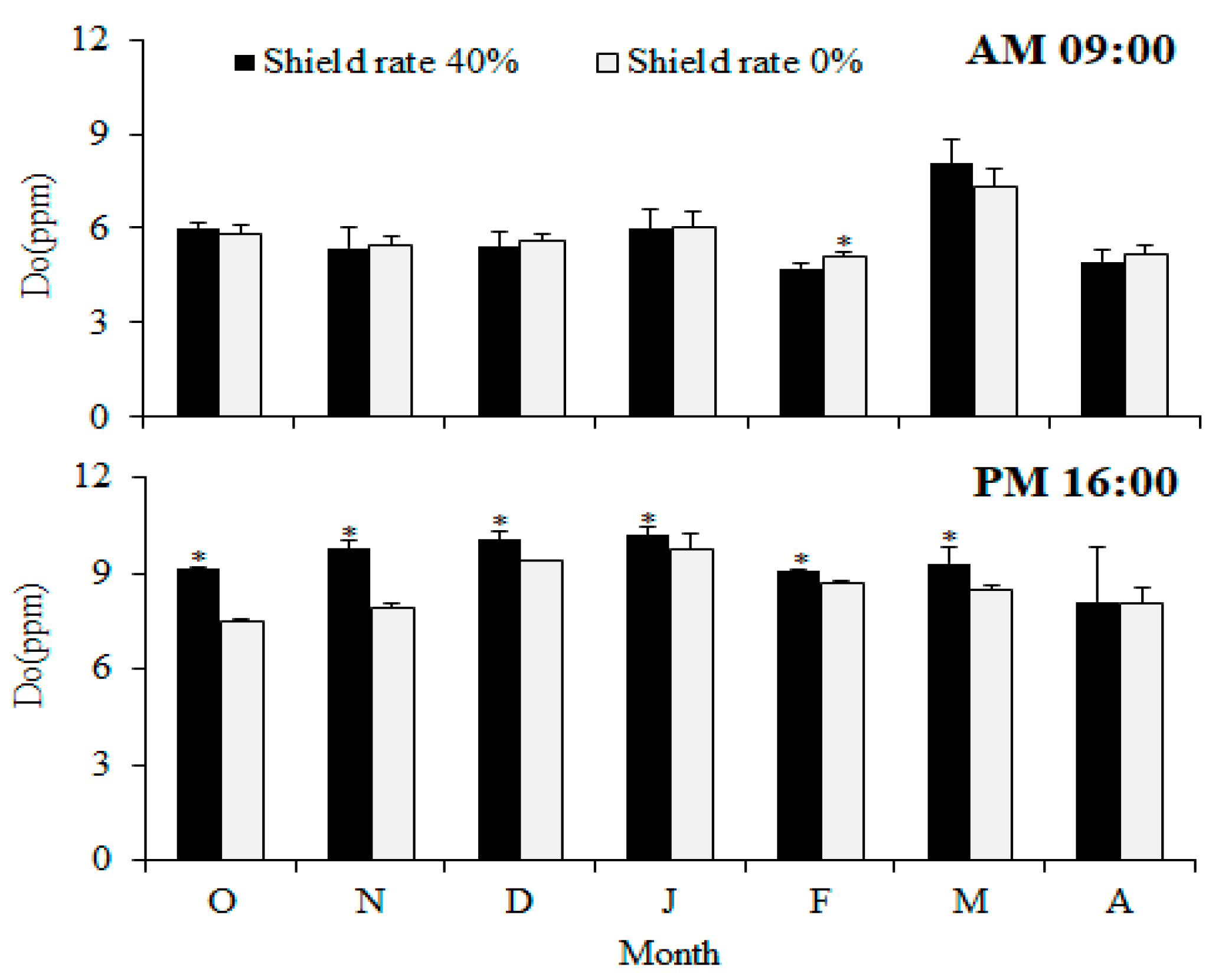
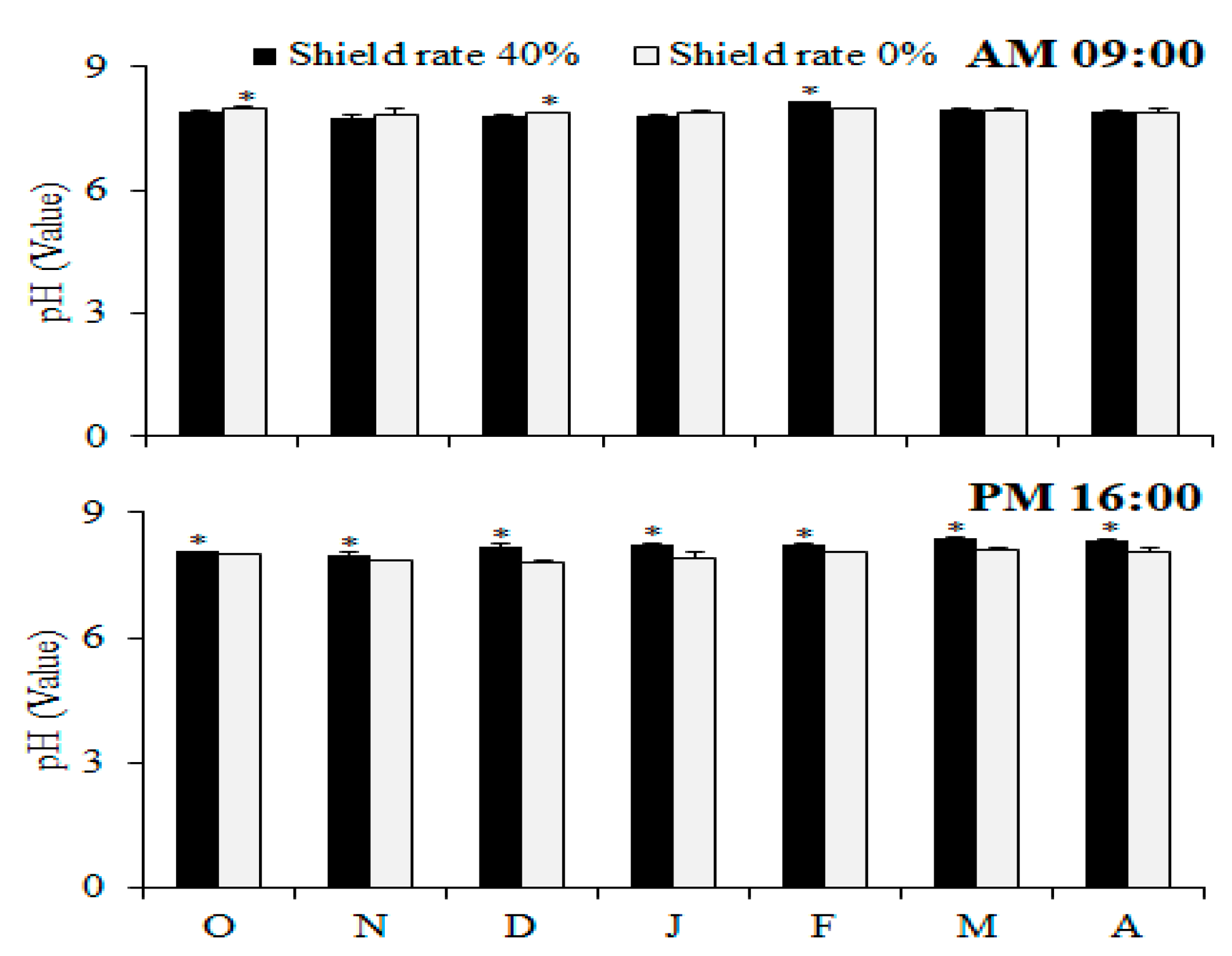
Previous studies have established a positive correlation between the pH and dissolved oxygen (DO) levels within water. As the aquaculture industry experiences rapid expansion across various countries, given the significance of factors pertaining to water quality, such as temperature, pH, and dissolved oxygen (DO), it has become progressively more essential to understand and manage them [
27,
28]. From October to April, the 40% shading group exhibited higher afternoon pH values, suggesting that the water temperature and dissolved oxygen parameters within the fishpond were relatively stable. A highly stable algae population can reduce the risk of algal blooms in the pond. This is mainly attributed to the smaller variations in pH and dissolved oxygen observed in the 40% shading group. The redox potential and pH value can be used to predict the water quality and assess the concentration of organic matter. During dry seasons, when the concentration of algae increases and they are agitated by the action of wind, the 0% shading treatment group exhibited higher dissolved oxygen levels (
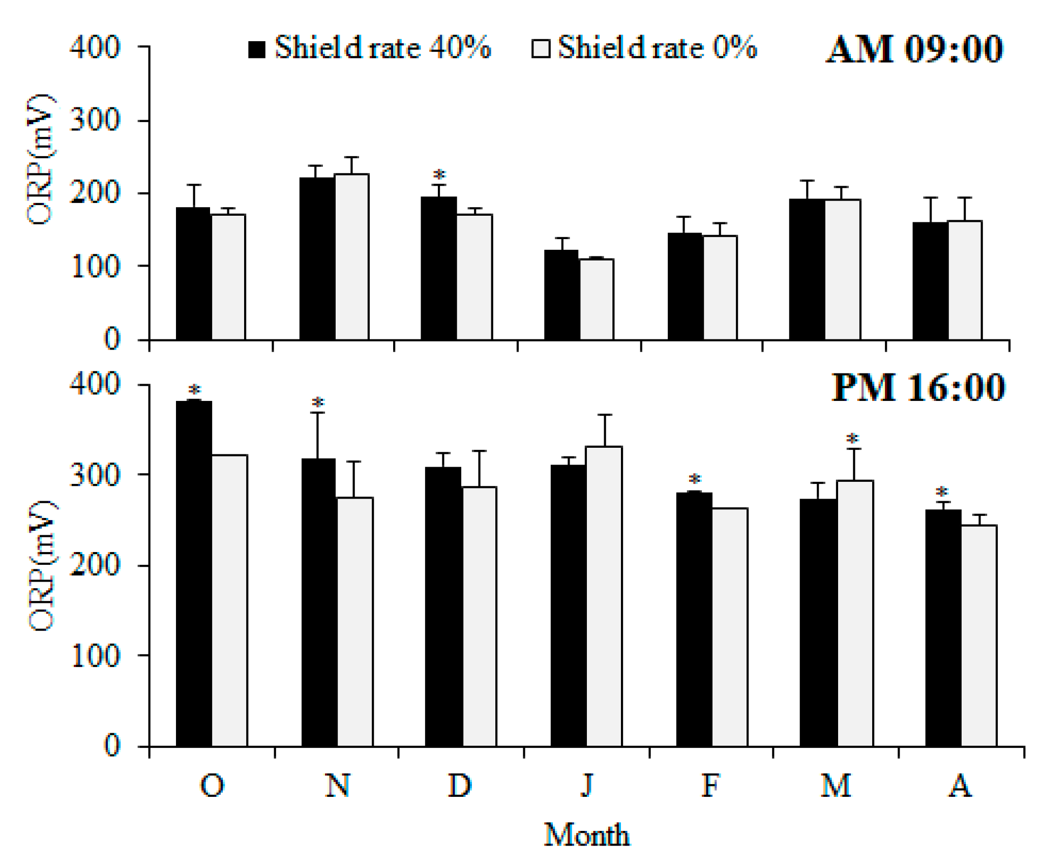
Figure 6). It was observed that the redox potential in the pond tended to rise with rainfall. Therefore, the months showing differences usually correspond with the rainy season. In a comparison of the monthly redox potentials, significant differences (
p < 0.05) were observed between the two groups from October to December 2018 and from February to April. At 09:00 in the morning, only December displayed a significant difference (
p < 0.05), while the remaining differences were found at 16:00 in the afternoon. This suggests that this time could serve as an optimal window for assessing the water quality. At 16:00 PM, the 0% shading group was higher only in March, showing a significant difference (
p < 0.05). Moreover, due to the onset of rain in March, with 74.5 mm of rainfall, a strong correlation was noted between significant changes in water quality and rainfall. From October to April, no significant differences (
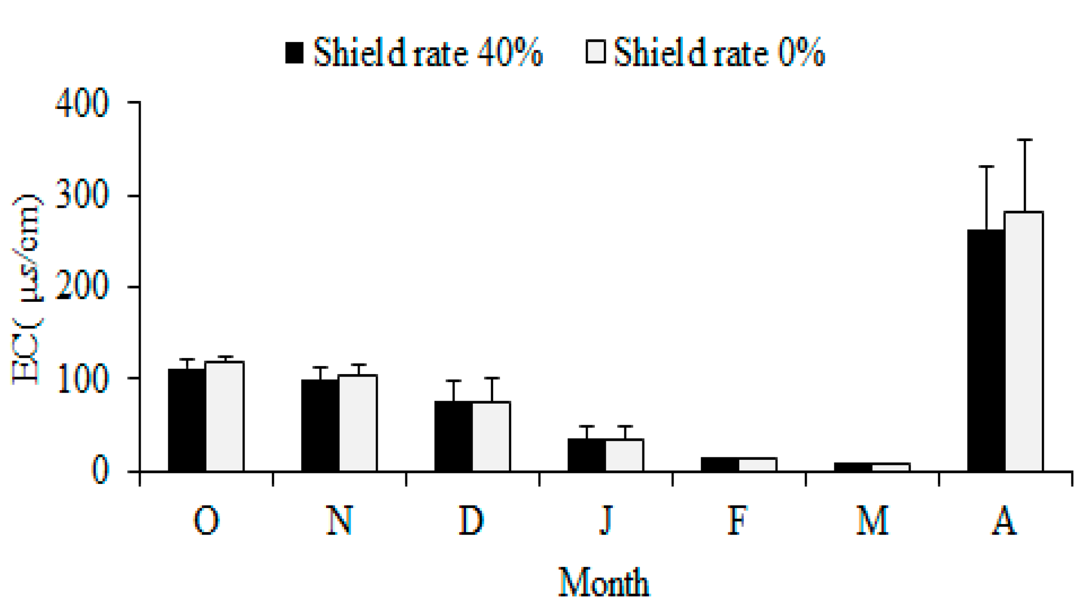
p > 0.05) were found in the values of conductivity between the two treatment groups. As depicted in the figures, from October to February of the subsequent year, there was virtually no rainfall, and the conductivity decreased progressively. This can be attributed to sunlight, temperature, and the concentration of algae in the water. As the temperature started to decrease in October, the conductivity reached its lowest point in February–March. This is primarily because during this period, the temperature is relatively low, reducing the feeding efficiency of fish and shrimp (
Figure 9). However, in April of the following year, as the farming period extended, the conductivity began to rise. When sunlight increased and the temperature rose, it led to a surge in feeding by aquatic organisms. As the temperature rose, the concentration of organic salts also increased. The seasonal shift in April resulted in a conductivity of >260 μs/cm, which was influenced by increased rainfall and feeding. However, throughout the year, the conductivity of the 0% shading group was slightly higher, but the difference between the two treatment groups reduced with the progression of the time of farming, and the conductivity began to increase in April. The lowest conductivity was recorded in February, during a period of cold, dry weather without rain, and the weather was relatively stable (
Figure 4).
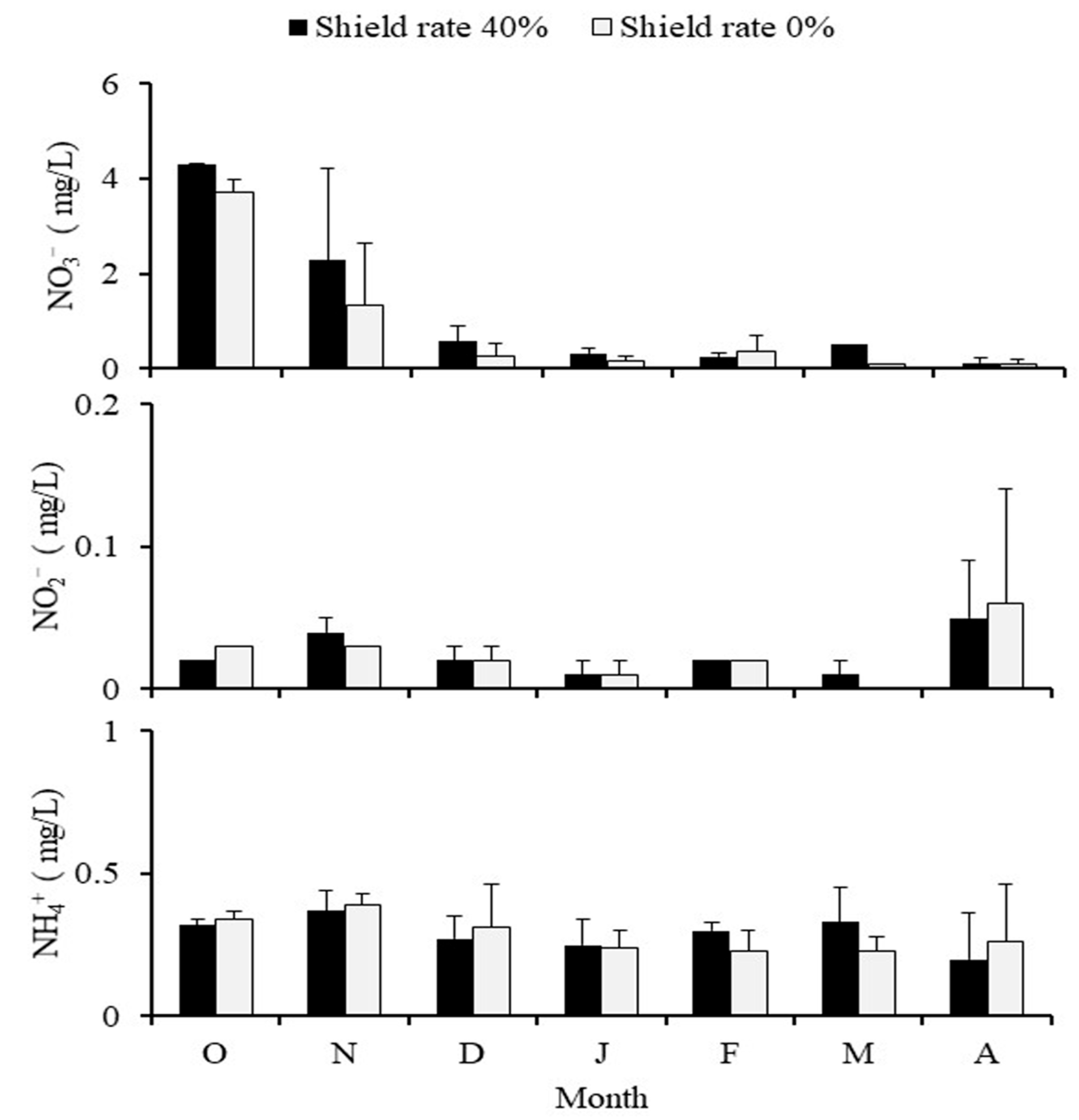
Monthly climatic variations were the reason for the higher nitrite levels in the 40% shading group from October to September. During the dry season from October to December, when rainfall is absent, the nitrite levels in the 0% shading group actually exceeded those of the 40% group, highlighting a significant difference. It is clear that the nitrite levels in the pond were substantially influenced by the amount of rainfall. In spring and summer, the nitrite levels in the 40% shading group were higher than those in the 0% shading group, primarily due to the vigorous photosynthesis in the 0% shading group, which effectively removed any nitrogenous waste in the pond. During this period, the 40% shading group, with a lower concentration of algae, was less equipped to handle nitrites. However, come autumn, the reduction in photosynthesis and the dramatic drop in salinity in the 40% shading group resulted in the mass die-off of algae, leading to higher nitrite levels in the 0% shading group. Consequently, the water quality became unstable, causing the fish to feed less frequently. In contrast, the 40% shading group recorded lower nitrite levels, mainly due to the lower base production and concentration of algae, resulting in a slower immediate change in water quality (
Figure 10). In spring and summer, the concentration of ammonia in the 40% shading group was higher than in the 0% shading group, largely because the 0% group, with its robust photosynthesis, was more adept at managing nitrogenous waste. In contrast, in fall and winter, the concentration of ammonia in the 40% shading group was higher. In the study area, blue-green algae and diatoms were observed as benthic algae. The primary species identified were
Lyngbya sp. and
Phormidium sp. As the year moved into autumn and the temperatures dropped, the algae gradually transitioned from green algae to diatoms, and the flipping of algae started to occur. Throughout the experiment, filamentous algae could be observed growing around the floating platforms in November. These algae serve as a part of the food source for fish and shrimp, thus augmenting the food supply for
L. vannamei. Floating photovoltaic systems offer a larger surface area for
L. vannamei to rest, improving the chances for
L. vannamei to attach, feed, hide, and molt. However, in the early morning, when the sun has yet to rise and photosynthesis has not started, the bulk of the floating photovoltaic system consumes some space, resulting in a reduced rate of water flow and lower dissolved oxygen levels in some areas of the pond. Therefore, in the future, it will be necessary to introduce oxygenation facilities to enhance the levels of dissolved oxygen.
Additionally, the relationship between the raft’s structure and water flow deserves attention. The system should be adjusted in response to the rate of water flow to minimize the buildup of suspended particles and mitigate the uneven distribution of water flow, thereby preventing the degradation of pond water and sediment quality. The number of times a significant number of algae perished was higher in the 0% shading group, causing C. chanos to cease feeding, and this was heavily affected by seasonal changes, which slowed their growth. Temperatures began to rise in April, and both the quantity and frequency of feedings increased. As a result, the waste produced by fish and shrimp grew, and the metabolic rate of the aquatic organisms accelerated, leading to a rise in the nitrite concentration. Eventually, it was discovered that the factors of water quality of the two treatment groups remained within safe limits during the farming process.
The main contribution of this study is that it elucidated the biotic and abiotic characteristics of floating photovoltaic systems combined with aquaculture, including changes in the growth of fish and shrimp, temperature, salinity, dissolved oxygen, and pH levels. This experiment involved the co-culture of
L. vannamei and
C. chanos. As well as the shading rates and water quality and cultivation conditions that were examined in this study, the observed growth of
L. vannamei and
C. chanos may also be affected by potential biotic factors, such as their species’ characteristics, life history, prey and predator species, and mortality rate. More experimentation with the farming of other aquatic organisms is needed in the future to gather data related to different species. The combination of floating photovoltaic systems with aquaculture not only enhances the added value of the aquaculture industry but also boosts the usage rate of the photovoltaic industry, stabilizes the supply of clean energy, and could provide a new avenue for the future development of aquaculture in Taiwan. This study investigated the growth and aquatic environmental factors of
L. vannamei and
C. chanos in a polyculture system under floating photovoltaic systems combined with aquaculture. The objective was to examine the dynamic changes in these environmental factors, aiming to enhance both the biological and abiotic yield and the production value of the solar photovoltaic–aquaculture industry. The results can serve as a valuable reference for stakeholders involved in this sector. In Tainan, Taiwan, the average time for effective daily power generation is approximately four hours. The water wheel in our system consumed 1.49 kW per day, while the feeder and the surveillance video system consumed 0.5 kW and 0.15 kW daily, respectively. The system’s total daily power consumption was 2.14 kW. Therefore, floating solar photovoltaic systems, which do not take up additional land resources, reduce the evaporation of water, suppress the proliferation of algae, and generate electricity for self-use, are suitable for the development of integrated aquaculture and photovoltaic systems. The process is susceptible to environmental and climatic changes. According to research by [
29], the performance of solar panels can be influenced by various environmental factors, especially the intensity of sunlight, cloud cover, and wind speed. Hence, the selection of the materials is particularly crucial, and the use of sturdy cables and anchoring systems can minimize issues that might affect aquaculture during this process. Additionally, in coastal areas with higher salinity, components that are resistant to corrosion, weathering, and oxidation can prevent the system from aging. The solar power generation system could sufficiently provide the electricity required for aquaculture, thus reducing the cost of electricity for this purpose. As a result, floating solar photovoltaic systems, which do not consume land resources, reduce water evaporation, inhibit algal blooms, and generate power for self-use, are well suited for the development of synergistic aquaculture–electric systems. The combined process of aquaculture and electricity generation can be easily affected by environmental and climate changes. A stable cable and anchoring system can minimize the potential impact on the process of aquaculture. Therefore, the choice of materials is of particular importance. Differences were observed in the growth of
C. chanos farmed in the combined aquaculture and electricity generation system and those farmed in the traditional farming system. Whether this difference is related to the disparities in light exposure and plankton during the farming process and whether there are differences in nutritional value are subjects that require further observation and research.
Taiwan, being densely populated and with a high energy demand in summer, has limited land suitable for the development of renewable energy. However, solar energy is ubiquitous in our lives. It can be widely utilized, is easily obtained, and it does not pollute the environment. Solar power generation is a zero-carbon, noise-free mode of producing electricity that can effectively reduce greenhouse gas emissions [
30]. However, substantial amounts of land are required to achieve a certain level of power generation [
31,
32]. In Taiwan, where the land is narrow and densely populated, suitable land for the development of solar power is limited [
33,
34]. Under the model of floating photovoltaic systems combined with aquaculture, the issue of land scarcity can be effectively alleviated. With the recent climate change due to global warming, the development of industries that balance green energy production with sustainable fisheries is of vital importance. Therefore, based on the current trends and conditions of Taiwan’s environment, it is appropriate to develop solar photovoltaic systems combined with aquaculture. This study also proved that
L. vannamei and
C. chanos can be co-cultured under floating solar photovoltaic systems. This demonstrates the potential of utilizing regulations and planning for large-scale aquaculture areas in the future.


