Internal Flow Phenomena of Two-Way Contra-Rotating Axial-Flow Pump-Turbine with Various Numbers of Blades in Pump Mode

Abstract

The focus of this paper is to investigate how various numbers of blades impact the performance of a two-way contra-rotating axial-flow pump-turbine when operating in pump mode. In order to meet the two-way operation of the pump-turbine, the front and rear impellers are mirror-symmetric with the same hydraulic model, which ensures the consistent performance of the forward and reverse working conditions. However, when the two-stage impellers have the same number of blades, the dynamic–dynamic interference can be severe, which can threaten the stability of the unit. The present study explores the use of two-stage impellers with varying numbers of blades as a means of enhancing the performance of tidal energy units. By conducting numerical simulations on the front and rear impellers under different flow rates in pump mode, the impact of increasing the number of blades in each stage on the external characteristics of the pump-turbine is revealed. The internal flow characteristics of different models are analyzed, and the impact of the number of blades on the vortex is studied. Different blade numbers will have a certain impact on the internal flow of the two-way contra-rotating axial-flow pump–turbine. Increasing the number of blades will affect the development of tip-leakage vortices and promote their intersection with the wake. In addition, changes in the number of blades will have an impact on the location of the leading edge (LE) water impact on the rear impeller, which in turn affects the contours of vorticity of the rear impeller near the LE and the location of the suction surface (SS) flow separation. The findings of this study offer valuable insights for future research on the operation of contra-rotating axial-flow pump-turbines.

1. Introduction

The progress and welfare of a society can be measured through its energy consumption. However, traditional energy sources have limitations and may not be able to meet the rising demand in the foreseeable future. Renewable energies have emerged as a crucial solution to meet the increasing demand for energy.

Interest in finding and producing sustainable energy alternatives is currently emerging, as awareness of the adverse environmental impact of fossil energy sources increases [1,2,3]. The vast resources of marine energy will contribute to our future energy needs [4,5]. Of the known marine renewable energy sources, waves and tides are two different types of resources considered available that have the potential to generate electricity in the future.

Tidal power stations have been using artificially created tidal phase differences and flowing through turbines to generate electricity for a relatively long time [6,7]. Early studies on tidal power stations focused on traditional one-way or two-way operations without a pump mode [8,9,10]. However, as tidal power stations have further developed, scholars have studied the potential energy gains that can result from the pump mode [11,12]. Yates et al. [12] found that the pumped energy gain is 6% at best with the addition of finite flow velocities, finite turbine and sluice capacities, and the same turbine and pump efficiencies. Reversible pump-turbines allow for greater flexibility in energy generation and storage, as they can pump water during low-demand periods and release it during high-demand periods to generate electricity [13]. The sea level rises and falls twice a day in most regions, with an average interval of approximately 12 h 25 min between the two tides. The change in sea level in a day is roughly like a sine wave, and the tidal power station will adjust the reservoir water level to generate power according to the change in sea-water level. Most of the current units used in tidal power plants are reversible pump-turbines, which have six functions, including two-way power generation, two-way pumping, and two-way sluice, as shown in Figure 1 [9]. This helps to balance the grid and ensure a steady supply of energy. However, the design and operation of these pump-turbines can be complex and require careful management to ensure their efficient and safe operation.

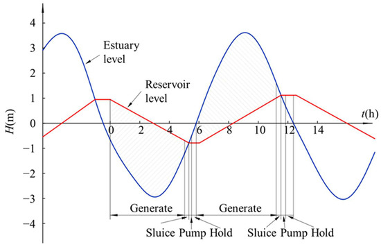
Figure 1. Six working conditions of a tidal power station.

Due to the operating circumstances of tidal power stations, the utilized reversible pump-turbines are forced into frequent switches between pumping and power generation modes. Hence, one of the most crucial research focuses is the flow instability of the unit. Contra-rotating axial-flow pumps offer significant advantages in terms of energy conversion, reduced pump size, and improved hydraulic and cavitation performance [14,15,16,17]. With further improvements, these pumps can also operate in both directions. Applying them in tidal power stations may be a promising direction for development.

Currently, most research on contra-rotating machinery has focused on fans and marine-current turbines. The University of Strathclyde has developed a novel contra-rotating tidal turbine and found that it can achieve reasonably good moored turbine stability within a real tidal stream [18].

Clarke et al. [19] have illustrated the design approach for downstream rotors by considering the flow angle from the upstream rotor. Lauria et al. used the Reynolds-averaged Navier–Stokes-equation (RANS) method and the OpenFOAM digital library to perform numerical calculations on several experiments with different platform angles. They obtained physical insights into jet characteristics and proposed a simple equation to predict the maximum dynamic head acting on the tail water [20]. On the basis of integrating the velocity distribution on the flow section of the partially full-flow inner bellows, Francesco et al. proposed a new flow calculation model, which considered the velocity distribution in the pressurized pipe to predict the velocity under the free surface-flow condition [21].

Mistry et al. [22] have explored the effect of axial spacing between rotors and found that different flow behavior is observed with variations in axial spacing for off-design speed combinations of rotor-1 and rotor-2. They have also determined that a high rotational speed of rotor-2 enables improved performance of the stage [23]. Airbus has conducted research on a contra-rotating open-rotor propulsion system and expects to achieve near-improvement in efficiency compared with modern turbofan engines [24].

Based on the previous research, this study utilized numerical simulation methods to investigate and analyze the performance of the contra-rotating axial-flow pump-turbine in pump mode. The influence of blade count on the performance of the contra-rotating axial-flow pump-turbine is analyzed by varying the blade count of the impeller. Additionally, the velocity field and vorticity of different blade counts at the rated flow rate were analyzed. The findings of this study provide valuable insights for further research on the design and operation of the contra-rotating axial-flow pump-turbine.

2. Materials and Methods

2.1. Pump Geometry

In this paper, we adopted the asymmetric blade design method, in which the β₁ and β₂ shown in Figure 2 are not equal. The front and rear impellers for the same hydraulic model mirror relationship, which can ensure the consistent performance of the forward and reverse working conditions, that is, to meet the requirements of a two-way operation. Table 1 shows the design parameters of the test pump, which uses a two-way design that eliminates the need to distinguish between flood and ebb modes during the simulation process for the impellers. The hydraulic model design parameters in Table 1 were designed using the streamline method and adopted an asymmetric design approach. Among them, the shroud and hub of the pump-turbine are both designed with cylindrical surfaces.

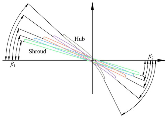
Figure 2. Blade airfoil angles.

Table 1. Design parameters of the test pump.

Design Parameters	Design Value
Flow Q (m3/h)	108
Head H (m)	1.25
Rotating speed n (r/min)	1450
Blade numbers	3
Impeller hub diameter (mm)	48
Impeller shroud diameter (mm)	145
Axial length of impeller blade outer flow line (mm)	36
Axial length of impeller blade inner flow line (mm)	42
Impeller blade thickness (mm)	3

2.2. Experimental Methods

To test and verify the design parameters, the test pump was manufactured according to the specified proportions. Figure 3a displays the impeller mold that was created using 3D-printing technology. A protective ring was installed around the impeller to ensure that the cast blade was accurate. This step is crucial in ensuring that the test results are reliable and can be used to make informed decisions about the design of the pump. Figure 3b shows the finished impeller.

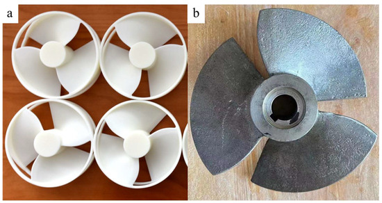
Figure 3. Impeller mold. (a) The 3D-printing mold of the impeller. (b) The actual impeller.

The experimental setup used in this research is a multi-functional testbed designed and built by the Fluid Mechanical Engineering Research Center of Jiangsu University and Jiangsu National Pump Co., Ltd (China, Jiangsu, Zhenjiang). The experimental setup includes a model pump, a buffer tank, valves I and II (gate valves), an electromagnetic flowmeter, two pressure sensors, and the corresponding pipeline. A schematic of the experimental setup is depicted in Figure 4.

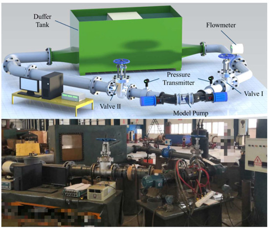
Figure 4. Schematic of the experimental setup.

2.3. Numeral Methods

2.3.1. Hydraulic Model Components

The calculation model of the two-way contra-rotating axial-flow pump is shown in Figure 5. The computational domain includes the suction, front diffuser, front impeller, mid-pipe, rear impeller, rear diffuser, and outpipe. It should be noted that the rotation axis of the two-stage impeller is collinear, but there are different rotation directions.

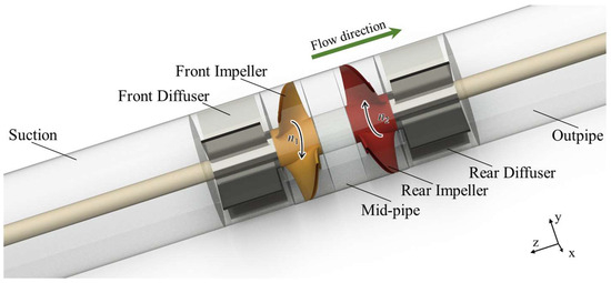
Figure 5. Domain of the hydraulic components.

2.3.2. Meshing

STAR CCM+ is applied to generate the mesh. Tip clearance of the grid is set to 0.3 mm. In our previous study [14], the grid independence analysis shows that the head change is under 0.1% when the number of grids exceeds 5.2 million.

The mesh in this paper adopts a finer near-wall mesh scale to ensure that the Y+ value of the near-wall mesh can be kept within 5. This can ensure the accuracy of the calculation of the near-wall area.

The grid scale near the wall was maintained, and the number of grids in the whole area was controlled by the maximum grid scale. Finally, two groups of schemes with the number of grid nodes being 31.25 million and 23.9 million, respectively, are obtained, which are named X1 (with 31.25 million grids) and X2 (with 23.9 million grids). On this basis, steady numerical simulation calculations were carried out on the two schemes, respectively, and the characteristic curves near the rated flow (108 m³/h) were obtained (shown in Figure 6). The computational machine we used has 2 intel Gold 6238R CPUs and 128 GB of RAM. When the 56 cores of the CPU are invoked, it takes about 8 h to complete a numerical simulation.

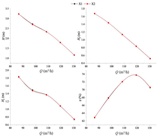
Figure 6. Grid number of the test pump.

Figure 7 shows the grid display of each region of X2. Mesh encryption is adopted on the inlet edge and the outlet edge of the guide vane blade and impeller blade, to ensure that the actual shape of the relevant region can be restored more accurately when the geometric domain is converted into a grid respectively. In addition, the tip area of the impeller blade is also encrypted, and the wall mesh near the tip gap adopts a lower mesh growth rate, and the number of mesh layers in this area is more than 25.

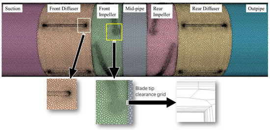
Figure 7. Computational grids.

2.3.3. Calculation Method and Boundary Conditions

In this paper, steady-state calculations and Realizable k-ε two-layer turbulence model are adopted [15]. It combines the Realizable k-ε turbulence model with the two-layer method. The transport equation of turbulent kinetic energy k and turbulent dissipation rate ε in the turbulence model k-ε is:

$$\frac{\partial }{\partial t}\left(\rho k\right)+\frac{\partial }{\partial x_i}\left(\rho k{u}_i\right)=\frac{\partial }{\partial x_j}\left[\left(\mu +\frac{{\mu }_t}{{\sigma }_k}\right)\frac{\partial k}{\partial x_j}\right]+P_k-\rho \left(\epsilon -{\epsilon }_0\right)$$

(1)

$$\frac{\partial }{\partial t}\left(\rho \epsilon \right)+\frac{\partial }{\partial x_i}\left(\rho \epsilon u_i\right)=\frac{\partial }{\partial x_j}\left[\left(\mu +\frac{{\mu }_t}{{\sigma }_{\epsilon }}\right)\frac{\partial \epsilon }{\partial x_j}\right]+\frac{\epsilon }{k}{C}_{\epsilon 1}{P}_{\epsilon }-C_{\epsilon 2}{f}_2\rho \left(\frac{{\epsilon }^2}{k}-\frac{{\epsilon }_0}{T_0}\right)$$

(2)

where p is the pressure, Pa; $u_i$ is the velocity in the i direction, m/s; μ is the laminar dynamic viscosity, kg/(m·s); ${\mu }_t$ is the turbulent eddy dynamic viscosity, kg/(m·s); and ρ is the water density at 25 ℃ with a value of 997 kg/m³. The liquid phase is 25 ℃ water with a dynamic viscosity of 8.899 × 10⁻⁴ kg/(m·s). ${\sigma }_k$ and ${\sigma }_{\epsilon }$ are the model coefficients. $C_{\epsilon 1}$ and $C_{\epsilon 2}$ are empirical constants. $P_k$ and $P_{\epsilon }$ are the production terms. ${\epsilon }_0$ is the ambient turbulence value that offsets turbulence attenuation. $f_2$ is the damping function. $T_0$ is the unit time scale.

The two-layer method was first proposed by Rodi [16] and divides the computing domain into two layers, namely the near-wall layer and the layer away from the wall. In the layer adjacent to the wall, the turbulence dissipation rate ε and turbulence eddy viscosity ${\mu }_t$ are specified as functions of the wall distance. The ε values specified in the near-wall layer are smoothly mixed with the values obtained from the transport equation away from the wall, and the turbulent kinetic energy equation for the entire basin is solved.

For the two-layer model, the near-wall dissipation rate is simply defined as:

$$\epsilon =\frac{k^{3/2}}{l_{\epsilon }}$$

(3)

where $l_{\epsilon }$ is the length scale function. According to the two-layer model variant described by Wolfstein [17],

$$l_{\epsilon }=C_{l}d\left[1-\exp \left(-\frac{{\mathrm{Re}}_d}{2C_l}\right)\right]$$

(4)

$$C_l=0.42C_{\mu }^{-3/4}$$

(5)

where $d$ is the distance to the wall.

${\mathrm{Re}}_d$ is the Reynolds number of the wall distance:

$${\mathrm{Re}}_d=\frac{\sqrt{k}d}{\nu }$$

(6)

where $\nu$ is the kinematic viscosity (m²/s).

$C_l$ and $C_{\mu }$ are the model coefficients. Based on the experimental measurement of the viscous sublayer of the boundary layer flow and the results of DNS (direct numerical simulation), the recommended value is 0.09 [25].

The wall proximity indicator proposed by Jongen [26] is used to combine the two-layer formula with the complete two-sided model:

$$\lambda =\frac{1}{2}\left[1+\tanh \left(\frac{{\mathrm{Re}}_d-{\mathrm{Re}}_y^{\ast }}{A}\right)\right]$$

(7)

where ${\mathrm{Re}}_y^{\ast }$ is the model coefficient with a default value of 60.$A$ can determine the width of the wall proximity indicator:

$$A=\frac{\left|\Delta {\mathrm{Re}}_y\right|}{\mathrm{atanh}0.98}$$

(8)

where $\Delta {\mathrm{Re}}_y$ is the model coefficient, and the default value is 10. Then, the turbulent viscosity ${\left.{\mu }_t\right|}_{k-\epsilon }$ in the Realizable k-ε turbulence model is mixed with the two-layer values to obtain the turbulent viscosity ${\mu }_t$ used in the Realizable k-ε turbulence model:

$${\left.{\mu }_t=\lambda {\mu }_t\right|}_{k-\epsilon }+\left(1-\lambda \right)\mu {\left(\frac{{\mu }_t}{\mu }\right)}_{2\mathrm{layer}}$$

(9)

The contra-rotating axial-flow pump-turbine has front and rear impellers that rotate in opposite directions. The calculation-domain inlet is a normal speed inlet, and the outlet is set as a pressure outlet. No-slip boundary conditions and smooth walls are used for the wall surfaces. A frozen rotor is used in the interface set during the steady-state numerical simulation. The residual target is set to 10⁻⁵.

2.3.4. Vorticity Equation

By considering the Navier–Stokes equation, the vorticity equation of the flow is as follows [27]:

$$\frac{D\stackrel{\rightharpoonup }{\omega }}{Dt}=\left(\stackrel{\rightharpoonup }{\omega }\cdot \nabla \right)\stackrel{\rightharpoonup }{u}-\stackrel{\rightharpoonup }{\omega }\left(\nabla \cdot \stackrel{\rightharpoonup }{u}\right)+\frac{\nabla \rho \times \nabla p}{{\rho }_{}^2}+\nu {\nabla }^2\stackrel{\rightharpoonup }{\omega }$$

(10)

where $\stackrel{\rightharpoonup }{\omega }$ is the vorticity, $\stackrel{\rightharpoonup }{u}$ is the velocity, $\nu$ is the kinematic viscosity, and $\nabla$ is the Hamiltonian operator. On the right side of Equation (10), these terms represent the vortex stretching, vortex dilatation, barotropic torque, and viscous diffusion, respectively. Since the medium being calculated in this paper is incompressible, the barotropic torque term is equal to 0. The Reynolds number is large, with an order of magnitude about 10⁶ near the blade tip, and the viscous diffusion term $\nu {\nabla }^2\stackrel{\rightharpoonup }{\omega }$ is relatively small to be typically disregarded. Thereafter, the Z-axis component of the vorticity equation is as follows:

$$\frac{D{\stackrel{\rightharpoonup }{\omega }}_Z}{Dt}={\left(\left(\stackrel{\rightharpoonup }{\omega }\cdot \nabla \right)\stackrel{\rightharpoonup }{u}\right)}_Z-{\stackrel{\rightharpoonup }{\omega }}_Z\left(\nabla \cdot \stackrel{\rightharpoonup }{u}\right)$$

(11)

3. Results and Discussion

3.1. Performance Test

Figure 8 shows the experimentally and numerically obtained Q–H curve and Q–η curve under pump mode. In the area of large flow rate, the simulated value will be slightly higher than the experimental value. However, the simulated value will be slightly lower than the experimental value in the low flow-rate area. The efficiency point obtained by numerical simulation is slightly higher than that obtained by experiment in the area of large flow rate. In general, the experimental data are close to the simulated data and have the same variation trend.

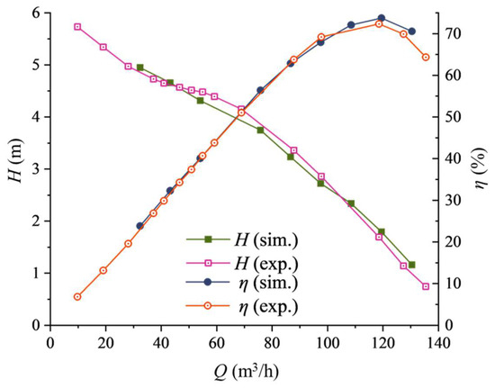
Figure 8. Performance curve under pump mode.

3.2. Research on the Various Numbers of Blades under Pump Mode

This paper uses two models for analysis, which differ in the number of blades. In Case1, both stages of the impeller have three blades. In Case2, the number of blades in the two stages is different, with three and four blades, respectively. The purpose of this is to improve the stability of the pump, similar to the principle of having different numbers in the impeller and guide vanes and without any multiple relationship between them. Due to the two-way operation, the two-stage impellers with different blade counts are no longer identical. Therefore, it is necessary to distinguish its flow direction. Case2a refers to the front impeller having four blades and the rear impeller having three blades, while Case2b is the opposite.

The Q–H curves of the different cases under the pump mode are shown in Figure 9. The Q–H curves of the different cases intersect near a flow rate of 119 m³/s. At low flow rates and rated flow rates (Q ≤ 108.5 m³/s), the head of Case2 is greater than that of Case. However, at high flow rates (Q > 108.5 m³/s), the head of Case2 is smaller than that of Case1. This means that when the blade count of a stage impeller of a contra-rotating axial-flow pump-turbine is increased, its Q–H curve becomes steeper. In all calculation conditions, the head of Case2b is greater than that of Case2a. This means that increasing the blade count of the rear impeller improves the head more than increasing the blade count of the front impeller.

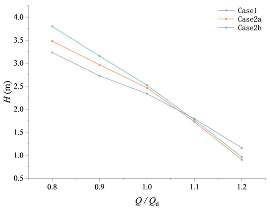
Figure 9. The Q–H curves of different cases under pump mode.

Figure 10 shows the Q–H curves of each stage impeller of the different cases under the pump operating conditions. H_f represents the power of the front impeller, and H_r represents the power of the rear impeller. In Case2a with a higher blade count for the front impeller, Q–H_f curve becomes steeper. The curves of Case1 and Case2b are almost identical until a flow rate of 86.66 m³/s, where the H_f of Case2b slightly increases. At low flow rates and rated flow rates (Q ≤ 108.5 m³/s), the head of Case2 is greater than that of Case1, especially for Case2b with 4 blades, which shows a significant improvement in the head.

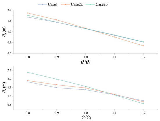
Figure 10. The Q–H curves of two-stage impellers of different cases under pump mode.

Figure 11 shows the Q–P curves of each stage impeller of the different cases under the pump mode. P_f represents the power of the primary impeller, and P_r represents the power of the secondary impeller. The Q–P curves of each stage impeller of the different cases under the pump mode have the same trend as the Q–H curves. Since the same motor is used for both stage impellers, it is important to focus on the power of the rear impeller, P_r. At low flow rates and rated flow rates (Q ≤ 108.5 m³/s), increasing the blade count, especially for the rear impeller, leads to a significant increase in P_r.

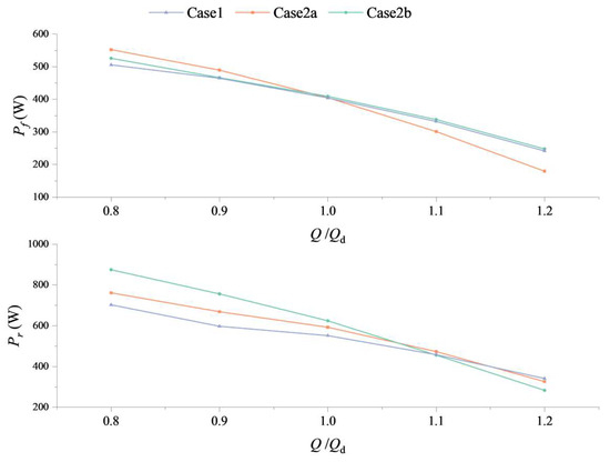
Figure 11. The Q–P curves of two-stage impellers of different cases under pump mode.

Figure 12 shows the Q–η_f/η_r curves of each stage impeller of the different cases under the pump operating conditions. Here, η_f represents the efficiency of the front impeller, and η_f represents the efficiency of the rear impeller. Case2a shows a significant change in η_f, especially at high flow rates where η_f drops significantly. The Q–η_f curves of Case1 and Case2b almost overlap in all conditions, indicating that the power output of the front impeller is the same with the same blade count in the front impeller. At low flow rates, the Q–η_r curve of Case2b is significantly improved. This indicates that increasing the blade count of the rear impeller can improve its efficiency at low flow rates. At high flow rates, all cases of Case2 show a significant decrease in efficiency, especially Case2b.

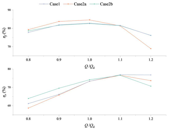
Figure 12. The Q–η_f/η_r curves of two-stage impellers of different cases under pump mode.

Figure 13 shows the Q–η curves of the different cases under the pump mode. At high flow rates (Q > 108.5 m³/s), the efficiency of Case2 decreases significantly, and the high-efficiency point of Case2 shifts toward low flow rates. In addition, from Case1 to Case2b to Case2a, the high-efficiency region of the unit under the pump mode gradually narrows. It is precisely because of the increase in the number of blades that the flow-section area decreases, which will cause greater flow obstruction at high flow rates. In Case2, a higher efficiency can be achieved by increasing the blade count of the front impeller. At low flow rates (Q < 108.5 m³/s), increasing the blade count of the rear impeller can achieve higher efficiency, while increasing the blade count of the front impeller has a negative impact on the efficiency of the unit.

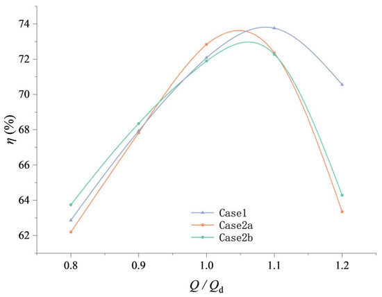
Figure 13. The Q–η curves of different cases under pump mode.

3.3. Streamline Analysis

Pump hydraulic performance and energy transfer characteristics will be significantly affected by changes in the flow pattern [28]. Figure 14 shows a schematic diagram of the impeller span surface. Span 1 represents a cylindrical surface with Span = 0.95, and Span 2 represents a cylindrical surface with Span = 0.6.

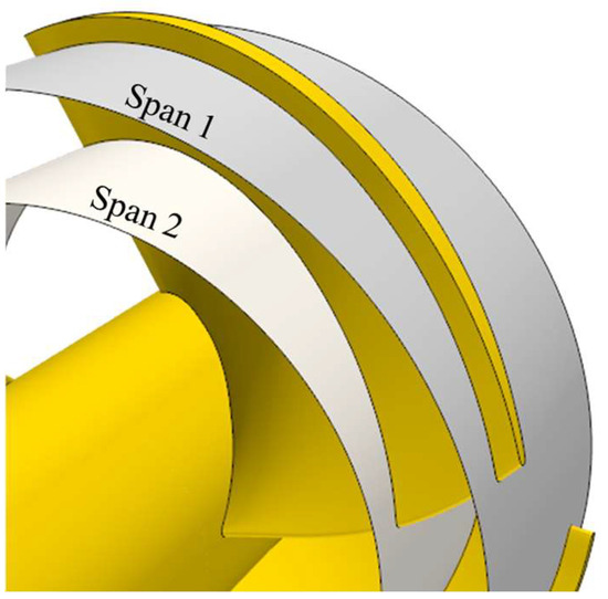
Figure 14. Span surface.

Figure 15 shows the streamlines of the Span 2 impeller flow field under the rated flow rate (Q = 108.5 m³/s) for the different cases. In the front impeller, it is difficult to observe significant differences in the streamlines. The red dashed box in Figure 15 represents the area near the LE (leading edge) of the secondary impeller, which is enlarged and shown in Figure 16 for better observation of the impact position of the fluid on the LE of the rear impeller. A red dashed line is added as a reference for the impact position. Compared with Case1, the impact position of Case2a shifts downstream, which is the main reason for the increase in the P_r of Case2a. When the two-stage impellers maintain the same speed, the impact position of the fluid on the rear impeller is not ideal. The impact position of Case2b shifts slightly upstream, which is actually beneficial for the impeller to work. However, the increase in blade count leads to an increase in power, so although the power of the rear impeller of Case2b is higher, its efficiency is not much different from that of Case1.

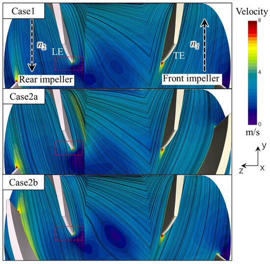
Figure 15. Streamline on Span 2.

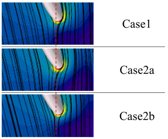
Figure 16. Streamline on Span 2 near the LE of the rear impeller blade.

To further investigate the flow characteristics of the two-stage impellers, this study extracted the velocity iso-surfaces of 11.5 m/s inside the front impeller and 15 m/s inside the rear impeller, as shown in Figure 17 and Figure 18, respectively. The higher velocity regions are mainly located on the suction surface near the LE of each stage impeller. In Figure 17, the 11.5 m/s velocity iso-surface of Case2a is significantly smaller than that of the other two cases, indicating that increasing the blade count of the front impeller can reduce the high-velocity region of the front impeller. Comparing this with Figure 12, it can be found that the efficiency η_f of the front impeller of Case2a is the highest at this condition. In Figure 18, the 15 m/s iso-surface area of Case2b is the largest. Comparing this with Figure 16, as the position of the fluid impact on the LE shifts downstream, the area of the 15 m/s iso-surface gradually decreases.

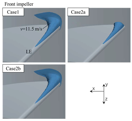
Figure 17. Iso-surface set on the front impeller blade.

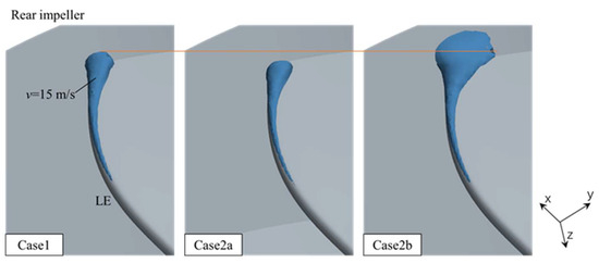
Figure 18. Iso-surface set on the rear impeller blade.

3.4. Vorticity Analysis

Figure 19 shows the contours of vorticity on Span 2 in Case1. Due to the large distance between Span 2 and the tip-clearance area, the change of vorticity caused by tip-clearance leakage cannot be observed. The vorticities are primarily a result of flow separation caused by the impact of water on the LE of the two-stage impeller, as well as vortices formed by the wake of the TE (trailing edge). However, the large contours of vorticity are not observed in the region between the two-stage impeller, so the focus of the next analysis is mainly on the inner region of the two-stage impeller. Ali Tafarojnoruz et al. found that downstream of the cylinder, the influence of the wake from the top of the cylinder is mainly limited to the area near the top of the cylinder, while the influence of the separated shear layers (SSLs) from the side of the cylinder dominates in a larger area, and the vorticity intensity related to the wake is mainly significant in the “very near wake” region [29].

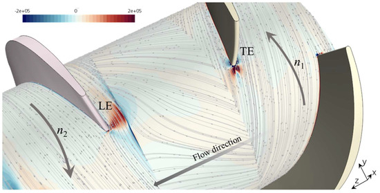
Figure 19. Contours of vorticity on Span 2.

Figure 20 displays the contours of the vorticity and each term on Span 1 of the front impeller. Notably, there is a region near the SS (suction surface) of the blade with a large absolute value of significant vorticity, which is located in close proximity to the tip clearance of the impeller. Along the flow direction, there is a trend of gradual diffusion in this area. This is due to vorticity caused by blade-tip leakage. As shown in Figure 20, the vorticity in this area is mainly dominated by the vortex stretching term, which means that the vortex deformation here is relatively severe. In addition, there are obvious vortices in the LE region, which are generated by the impact of the fluid on the LE. There is a region with a small value of vorticity near the PS (pressure surface) in the LE, which is a continuation of the vortex caused by impact downstream and gradually dissipates in the flow. Comparing Figure 20a with Figure 20b, only a slight difference near the blade is observed. That is, in the region near the tip of the blade, the vortex stretching term in the vorticity transport equation is dominant. The contours of the vorticity caused by the vortex stretching term is mainly located near the blade surface and in the wake near the TE.

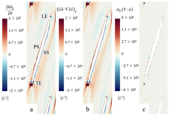
Figure 20. Contours of vorticity and each term on Span 1 of the front impeller. (a) The distribution of the vorticity on Span 1. (b) The contours of the vortex stretching term on Span 1. (c) The contours of the vortex dilatation term on Span 1.

Figure 21 shows the contours of the vorticity and each term on Span 2 of the front impeller. At this time, the regions with a large absolute value of significant vorticity are mainly in the wake regions near the LE and the TE. There is a region with a small value of vorticity near the blade surface in Figure 21, which means that the vortex stretching term still dominates the vorticity transport equation at this time.

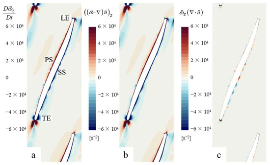
Figure 21. Contours of vorticity and each term on Span 2 of the front impeller. (a) The distribution of the vorticity on Span 2. (b) The contours of the vortex stretching term on Span 2. (c) The contours of the vortex dilatation term on Span 2.

Figure 22 shows the contours of vorticity on Span 1 of the front impeller of the different cases. Figure 22a,c have almost identical contours of vorticity. In Figure 22b, due to the increase in the number of blades, the contours of vorticity caused by blade-tip leakage near the SS increases significantly and intersects in the wake region. A significant negative vorticity occurred downstream of the TE of the front impeller of Case2a.

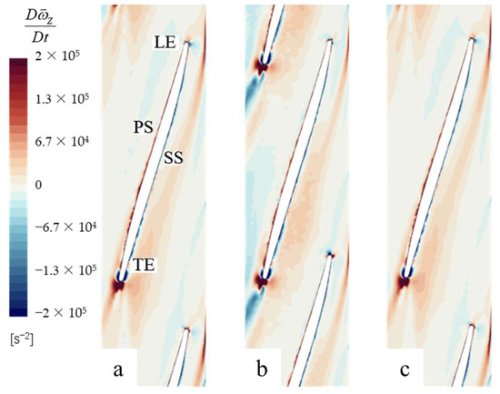
Figure 22. Contours of vorticity on Span 1 of the front impeller of different cases: (a) Case1; (b) Case2a; (c) Case2b.

In Figure 23, the significant difference is not observed in the contours of vorticity around the impeller, which means that the change in the number of blades mainly affects the vorticity caused by blade-tip leakage. This is mainly due to the reduction of a single flow path caused by the increase in the number of blades, limiting the development of tip-leakage vortices toward adjacent blades, promoting their downward development and converging with the wake of the TE.

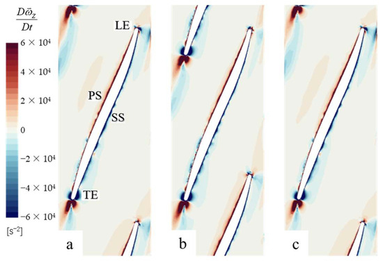
Figure 23. Contours of vorticity on Span 2 of the front impeller of different cases: (a) Case1; (b) Case2a; (c) Case2b.

Figure 24 shows the contours of vorticity on Span 1 of the rear impeller of the different cases. As shown in Figure 24, the position of the LE water impact on the rear impeller has shifted, resulting in a significant difference in the contours of vorticity at the LE. Compared with other cases in Figure 24c, Case2b has the smallest vorticity distributions and the smallest impact loss. Similar to the front impeller, the wake of Case2b with more blade numbers is also significantly different from the other two models.

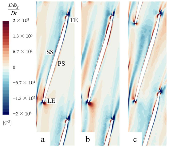
Figure 24. Contours of vorticity on Span 1 of the rear impeller of different cases: (a) Case1; (b) Case2a; (c) Case2b.

Figure 25 shows the contours of vorticity on Span 2 of the rear impeller of the different cases. The difference in the contours of vorticity in this region is caused by the displacement of the position of the LE water impact on the rear impeller. In addition, vortices generated by the LE water impact will develop downstream along the watershed near the SS in Case1. In Case2, the SS of the rear impeller will have higher contours of vorticity at a position 1/3 of the blade-line length from the LE, which means that flow separation will occur at this position. However, the position of the outflow only appears in the area where the SS is close to the TE in Case1.

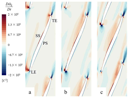
Figure 25. Contours of vorticity on Span 2 of the rear impeller of different cases: (a) Case1; (b) Case2a; (c) Case2b.

In summary, different blade numbers will have a certain impact on the internal flow of the two-way contra-rotating axial-flow pump–turbine. Increasing the number of blades will affect the development of tip-leakage vortices and promote their intersection with the wake. In addition, changes in the number of blades will have an impact on the location of the LE water impact on the rear impeller, which in turn affects the contours of vorticity of the rear impeller near the LE and the location of the SS flow separation.

4. Conclusions

In order to improve the stability of the two-way contra-rotating axial-flow pump-turbine, the blade count of the impeller was adjusted by using a two-stage impeller with different blade counts. Based on this, the internal flow phenomena of the two-stage impeller were studied, and the following conclusions were drawn.

• An increase in the blade count of the impeller stage of a mixed-flow pump-turbine will result in a steeper Q–H curve. Increasing the blade count of the impeller stage has a greater effect on improving the head than increasing the blade count of the previous stage.
• With the increase in the number of impeller blades of a certain stage in the contra-rotating axial-flow pump, the high-efficiency point of the unit under pump mode will shift toward lower flow rates, and the high-efficiency region will also become narrower.
• Varying the number of blades will have an impact on the location of the LE water impact on the rear impeller, which in turn affects the contours of vorticity of the rear impeller near the LE.

This article compares and analyzes the impact of changing the number of blades or speed of a certain stage impeller of a bidirectional counter-rotating water pump-turbine using the same hydraulic model on the performance of the unit. The results indicate that increasing the number of blades in a single stage impeller can result in a steeper head curve, significantly improving the hump phenomenon of the secondary impeller, but also leading to a narrower efficient zone of the unit. The findings of this study offer valuable insights for future research on the operation of contra-rotating axial-flow pump-turbines.

References

- Sangiuliano, S.J. Community energy and emissions planning for tidal current turbines: A case study of the municipalities of the Southern Gulf Islands Region, British Columbia. Renew. Sustain. Energy Rev. 2017, 76, 1–8. [Google Scholar]
- Li, Y.; Lence, B.J.; Calisal, S.M. An integrated model for estimating energy cost of a tidal current turbine farm. Energy Convers. Manag. 2011, 52, 1677–1687. [Google Scholar]
- Qian, P.; Feng, B.; Liu, H.; Tian, X.; Si, Y.; Zhang, D. Review on configuration and control methods of tidal current turbines. Renew. Sustain. Energy Rev. 2019, 108, 125–139. [Google Scholar]
- Kim, K.; Ahmed, M.R.; Lee, Y. Efficiency improvement of a tidal current turbine utilizing a larger area of channel. Renew. Energy 2012, 48, 557–564. [Google Scholar]
- Charlier, R.H. A “sleeper” awakes: Tidal current power. Renew. Sustain. Energy Rev. 2003, 7, 515–529. [Google Scholar]
- Neill, S.P.; Angeloudis, A.; Robins, P.E.; Walkington, I.; Ward, S.L.; Masters, I.; Lewis, M.J.; Piano, M.; Avdis, A.; Piggot, M.D.; et al. Tidal range energy resource and optimization—Past perspectives and future challenges. Renew. Energy 2018, 127, 763–778. [Google Scholar]
- Angeloudis, A.; Falconer, R.A. Sensitivity of tidal lagoon and barrage hydrodynamic impacts and energy outputs to operational characteristics. Renew. Energy 2017, 114, 337–351. [Google Scholar]
- Prandle, D. Simple theory for designing tidal power schemes. Adv. Water Resour. 1984, 7, 21–27. [Google Scholar] [CrossRef]
- Burrows, R.; Walkington, I.; Yates, N.C.; Hedges, T.S.; Wolf, J.; Holt, J.T. The tidal range energy potential of the West Coast of the United Kingdom. Appl. Ocean. Res. 2009, 31, 229–238. [Google Scholar]
- Xia, J.; Falconer, R.A.; Lin, B. Impact of different tidal renewable energy projects on the hydrodynamic processes in the Severn Estuary, UK. Ocean. Model. 2010, 32, 86–104. [Google Scholar]
- Mackay, D.J.C.; Hafemeister, D. Sustainable Energy-Without the Hot Air. Am. J. Phys. 2010, 78, 222–223. [Google Scholar]
- Yates, N.; Walkington, I.; Burrows, R.; Wolf, J. The energy gains realisable through pumping for tidal range energy schemes. Renew. Energy 2013, 58, 79–84. [Google Scholar] [CrossRef]
- Harcourt, F.; Angeloudis, A.; Piggott, M.D. Utilising the flexible generation potential of tidal range power plants to optimise economic value. Appl. Energy 2019, 237, 873–884. [Google Scholar] [CrossRef]
- An, C.; Chen, Y.; Zhu, R.; Wang, X.; Yang, Y.; Shi, J. Internal Flow Phenomena of Two-Way Contra-Rotating Axial Flow Pump-Turbine in Pump Mode under Variable Speed. J. Appl. Fluid Mech. 2023, 16, 285–297. [Google Scholar] [CrossRef]
- Shih, T.-H.; Liou, W.W.; Shabbir, A.; Yang, Z.; Zhu, J.J.C. A new k-ϵ eddy viscosity model for high reynolds number turbulent flows. Comput. Fluids 1995, 24, 227–238. [Google Scholar] [CrossRef]
- Rodi, W. Experience with two-layer models combining the k-epsilon model with a one-equation model near the wall. In Proceedings of the 29th Aerospace Sciences Meeting, Reno, NV, USA, 7–10 January 1991; p. 216. [Google Scholar]
- Wolfshtein, M. The velocity and temperature distribution in one-dimensional flow with turbulence augmentation and pressure gradient. Int. J. Heat Mass Transf. 1969, 12, 301–318. [Google Scholar] [CrossRef]
- Clarke, J.A.; Connor, G.; Grant, A.; Johnstone, C.; Ordonez Sanchez, S. Contra-rotating marine current turbines: Single point tethered floating system-stabilty and performance. In Proceedings of the 8th European Wave and Tidal Energy Conference, EWTEC 2009, Uppsala, Sweden, 7–11 September 2009. [Google Scholar]
- Clarke, J.A.; Connor, G.; Grant, A.; Johnstone, C. Design and testing of a contra-rotating tidal current turbine, Proceedings of the Institution of Mechanical Engineers. Part A J. Power Energy 2007, 221, 171–179. [Google Scholar] [CrossRef]
- Agostino, L.; Alfonsi, G.; Tafarojnoruz, A. Flow Pressure Behavior Downstream of Ski Jumps. Fluids 2020, 5, 14. [Google Scholar]
- Calomino, F.; Alfonsi, G.; Gaudio, R.; D’Ippolito, A.; Lauria, A.; Tafarojnoruz, A.; Artese, S. Experimental and Numerical Study of Free-Surface Flows in a Corrugated Pipe. Water 2018, 10, 638. [Google Scholar] [CrossRef]
- Mistry, C.; Pradeep, A. Effect of variation in axial spacing and rotor speed combinations on the performance of a high aspect ratio contra-rotating axial fan stage. Proc. Inst. Mech. Eng. Part A J. Power Energy 2013, 227, 138–146. [Google Scholar] [CrossRef]
- Mistry, C.; Pradeep, A. Influence of circumferential inflow distortion on the performance of a low speed, high aspect ratio contra rotating axial fan. J. Turbomach. 2014, 136, 071009. [Google Scholar] [CrossRef]
- Stuermer, A.W.; Akkermans, R.A. Validation of aerodynamic and aeroacoustic simulations of contra-rotating open rotors at low-speed flight conditions. In Proceedings of the 32nd AIAA Applied Aerodynamics Conference, Atlanta, GA, USA, 16–20 June 2014; The American Institute of Aeronautics and Astronautics: San Diego, CA, USA, 2014; pp. 16–20. [Google Scholar]
- Shih, T.-H.; Liou, W.W.; Shabbir, A.; Yang, Z.; Zhu, J. A New K-Epsilon Eddy Viscosity Model for High Reynolds Number Turbulent Flows: Model Development and Validation; NASA NTRS: Seattle, WA, USA, 1994. [Google Scholar]
- Jongen, T. Simulation and Modeling of Turbulent Incompressible Flows. Ph.D. Thesis, Swiss Federal Institute of Technology in Lausanne, Lausanne, Switzerland, 1998. [Google Scholar]
- Yu, Z. Numerical and Physical Investigation of Tip Leakage Vortex Cavitating Flows; Beijing Institute of Technology: Beijing, China, 2016. [Google Scholar]
- Li, X.; Chen, B.; Luo, X.; Zhu, Z. Effects of flow pattern on hydraulic performance and energy conversion characterisation in a centrifugal pump. Renew. Energy 2020, 151, 475–487. [Google Scholar] [CrossRef]
- Ali, T.; Lauria, A. Large eddy simulation of the turbulent flow field around a submerged pile within a scour hole under current condition. Coast. Eng. J. 2020, 62, 489–503. [Google Scholar]
Disclaimer/Publisher’s Note: The statements, opinions and data contained in all publications are solely those of the individual author(s) and contributor(s) and not of MDPI and/or the editor(s). MDPI and/or the editor(s) disclaim responsibility for any injury to people or property resulting from any ideas, methods, instructions or products referred to in the content. |
© 2023 by the authors. Licensee MDPI, Basel, Switzerland. This article is an open access article distributed under the terms and conditions of the Creative Commons Attribution (CC BY) license (https://creativecommons.org/licenses/by/4.0/).