Article

Impact of Vegetation Differences on Shallow Landslides: A Case Study in Aso, Japan

Department of Civil and Environmental Engineering, Faculty of Advanced Science and Technology, Kumamoto University, Chuo-ku, Kumamoto 860-8555, Japan
*
Author to whom correspondence should be addressed.
Water 2023, 15(18), 3193; https://doi.org/10.3390/w15183193
Submission received: 9 August 2023 / Revised: 30 August 2023 / Accepted: 1 September 2023 / Published: 7 September 2023
(This article belongs to the Topic Landslide Prediction, Monitoring and Early Warning)

Abstract

:
Climate change has increased the frequency and scale of heavy rainfall, increasing the risk of shallow landslides due to heavy rainfall. In recent years, ecosystem-based disaster risk reduction (Eco-DRR) has attracted attention as one way to reduce disaster risks. Vegetation is known to increase soil strength through its root system and reduce the risk of shallow landslides. To reduce the risk of shallow landslides using vegetation, it is necessary to quantitatively evaluate the effects that vegetation has on shallow landslides. In this study, we constructed a generalized linear model (GLM) and random forest (RF) model to quantitatively evaluate the impact of differences in the vegetation, such as grasslands and forests, on the occurrence of shallow landslides using statistical methods. The model that resulted in the lowest AIC in the GLM included elevation, slope angle, slope aspect, undulation, TWI, geology, and vegetation as primary factors, and the hourly rainfall as a trigger factor. The slope angle, undulation, and hourly rainfall were selected as significant explanatory variables that contribute positively to shallow landslides. On the other hand, elevation and TWI were selected as significant explanatory variables that contribute negatively to shallow landslides. Significant differences were observed among multiple categories of vegetation. The probability of shallow landslide in secondary grasslands was approximately three times that of coniferous and broadleaf forests, and approximately nine times that of broadleaf secondary forests. The landslide probability of shrubs was approximately four times that of coniferous and broadleaf forests, and approximately ten times that of broadleaf secondary forests. The results of constructing the RF model showed that the importance was highest for the hourly rainfall, followed by geology, then elevation. AUC values for the GLM and RF model were 0.91 and 0.95, respectively, indicating that highly accurate models were constructed. We quantitatively showed the impact of differences in vegetation on shallow landslides. The knowledge obtained in this study will be essential for considering appropriate vegetation management to reduce the risk of future shallow landslides.

1. Introduction

In recent years, climate change has been intensifying, leading to an increasing occurrence of abnormal weather patterns worldwide. As a result of climate change, the frequency and magnitude of heavy rainfall events have increased, leading to a rising trend in the occurrence of slope failures triggered by these extreme rain events. Among these slope failures, shallow landslides, which are phenomena where the topsoil layer on the slope bedrock detaches and moves downslope, can be regarded as the most common type of disaster on slopes [1]. Moreover, shallow landslides can affect human activities and cause damage to societal infrastructure [2]. We need to take measures to reduce the risk of these disasters.
Shallow landslides are caused by various factors, such as topography, geology, and vegetation [1]. Among these factors, it has been reported that vegetation greatly influences the occurrence of shallow landslides [3]. Vegetation can enhance the stability of slopes by increasing soil strength through their root systems [4,5]. However, its effect is considered limited for failures occurring deeper than the root system [6]. The concept of utilizing the functions of ecosystems such as vegetation for disaster prevention and mitigation is known as ecosystem-based disaster risk reduction (Eco-DRR), and discussions towards its implementation have been held in recent years [7]. To reduce the risk of shallow landslides using vegetation, it is necessary to quantitatively assess the influence factors that vegetation has on shallow landslides. Broadly speaking, the methods to evaluate the influence of vegetation factors on shallow landslides can be divided into two categories: analytical methods using slope stability models and statistical methods using statistical analysis or machine learning.
In analytical methods, the reinforcing effect due to root systems is assumed to be uniformly distributed along the slip surface in order to evaluate the impact of vegetation on slope stability [8,9]. However, recent studies have shown that the reinforcing effect due to root systems varies spatially and temporally [10,11]. The effect of root systems is distinguished by the direction of stress on the shear plane and is divided into vertical roots that pass through the landslide plane and horizontal roots that pass through the sidewalls around the landslide [4,12]. The reinforcing effect of vertical roots is most effective when uniformly present on the landslide plane [4], and the reinforcing effect of horizontal roots is reported to depend on the spatial distribution of roots [13]. Schwarz et al. [14] have proposed a model (Root Bundle Model, RBM) to incorporate the spatial distribution of the reinforcing effect due to root systems into slope stability analysis, and it has been used in many previous studies [15,16,17]. Thus, the effects of root systems are gradually being clarified through analytical methods. However, to evaluate the impact of vegetation on slope stability at the watershed scale using a physical model, a large amount of detailed data is required, which entails significant costs [18].
With the advancement in the preparation of GIS data, information on multiple factors, including vegetation, topography, geology, and rainfall, has become relatively easily accessible. Statistical methods are suitable for predicting and assessing surface landslides on a watershed scale [19]. Consequently, in recent years, there have been studies that statistically analyzed the causes of surface landslides and predicted the likelihood of future occurrences based on past landslide events [20,21]. The methods employed often include generalized linear models, random forests, and support vector machines [2,22,23]. However, in many previous studies, vegetation has only been incorporated into models as a single factor, without considering differences in vegetation types, such as forests, grasslands, and shrubs [20,24,25]. Focusing on forests, Moos et al. [26] introduced variables related to forest structure into their model and quantitatively demonstrated the impact of forest structure on slope stability. Zhang et al. [27] incorporated detailed forest-related information, such as tree age and species, into their model and showed that natural forests have a greater effect in suppressing shallow landslides than artificial forests. Thus, there are several studies that have focused on forests and statistically analyzed the relationship between the state of the forest and surface landslides. Focusing on grasslands, while there are not studies that have evaluated the impact of grassland conditions on shallow landslides using statistical methods, there are studies that have clarified the impact of grassland types on slope stability through mechanical analysis [28,29].
The Aso region in Japan possesses one of the world’s largest calderas, stretching approximately 25 km north–south and 18 km east–west. The caldera and its surroundings are covered by the largest grassland in Japan, spanning about 220 km2 [30]. This grassland has been maintained for more than 30,000 years through periodic anthropogenic burns [31]. However, since the 1960s, there has been a rapid decline in these grasslands due to factors such as the decline of the livestock industry, leading to abandoned grasslands, and the increase in afforestation policies that have resulted in a rise in artificially planted forests [32]. Such changes in vegetation have been shown to impact slope stability [33]. Therefore, in the Aso region where grasslands are transitioning to forests, evaluating the impact of vegetation differences, such as between forests and grasslands, on shallow landslides is crucial in providing information for optimal vegetation management aimed at reducing landslide risks.
On the relationship between vegetation differences such as forests and grasslands and shallow landslides, Kokutse et al. [34] reported that slope stability increased by 7.1% for grasslands and 18.7% for mature forests when compared to a vegetation-less condition, based on physical model analyses of four types of vegetation states, including grasslands and mature forests. Liu et al. [6] stated that both forests and grasslands have a function that increases slope stability, irrespective of the soil moisture content on the slope. On the other hand, Koyanagi et al. [35] conducted an assessment of the distribution and scale of landslides that occurred in forests and grasslands during the Kumamoto earthquake, indicating that landslides in grasslands occurred in steeper areas than those in forests. Kamp et al. [36] reported that the proportions of landslide areas in grasslands and forests in the landslides that occurred during the 2005 Kashmir earthquake were 3.8% and 0.1%, respectively. However, these studies did not take into account multiple factors that influence slope stability, such as topography, geology, and rainfall. Therefore, in this study, we focused on statistical methods that allow for the incorporation of multiple factors into the model. Our objective was to quantitatively evaluate the impact of vegetation differences, such as between grasslands and forests, on the occurrence of shallow landslides, and we aimed to provide essential information for optimal vegetation management and the formulation of strategic disaster mitigation and prevention plans to reduce the risk of shallow landslides. It should be noted that while shallow landslides can also occur due to earthquakes, this study focused on those caused by heavy rain, which occurs more frequently.

2. Study Area

The Aso region is located in the upper reaches of the Shirakawa basin in Kumamoto prefecture, Japan (Figure 1). The total study area was approximately 376 km2, with maximum and minimum elevations of 1591 m and 232 m, respectively. The average annual temperature observed at the AMeDAS (Automated Meteorological Data Acquisition System) Aso Otohime station from 1991 to 2020 is approximately 13 °C, with an annual rainfall of approximately 3000 mm, indicating that the study area receives a high amount of precipitation. Aso mountain is located almost in the center of the study area. To the north of Aso mountain lies the Asodani valley, while the south side is called the Nangodani valley. The Kurokawa river, a tributary of the Shirakawa river, flows through the Asodani valley, and the main stream of the Shirakawa river flows through the Nangodani valley. Polemonium kiushianum, a plant classified as critically endangered (IA category), grows in these grasslands. Furthermore, Sophora flavescens grows in the grasslands and serves as the food plant for the butterfly species Shijimiaeoides divinus, which is listed as endangered (IB). Therefore, these grasslands harbor various fauna and flora. Grasslands are dominated by Miscanthus sinensis with lesser amounts of Pleioblastus argenteostriatus [36].
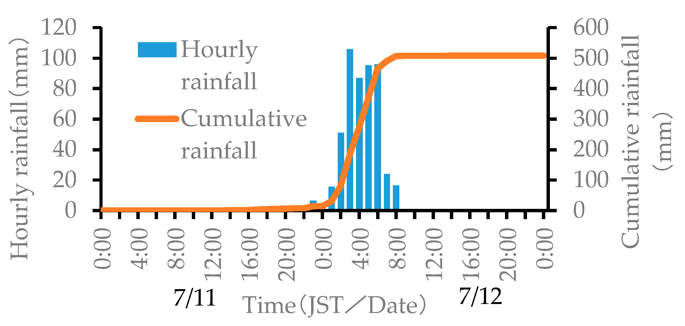
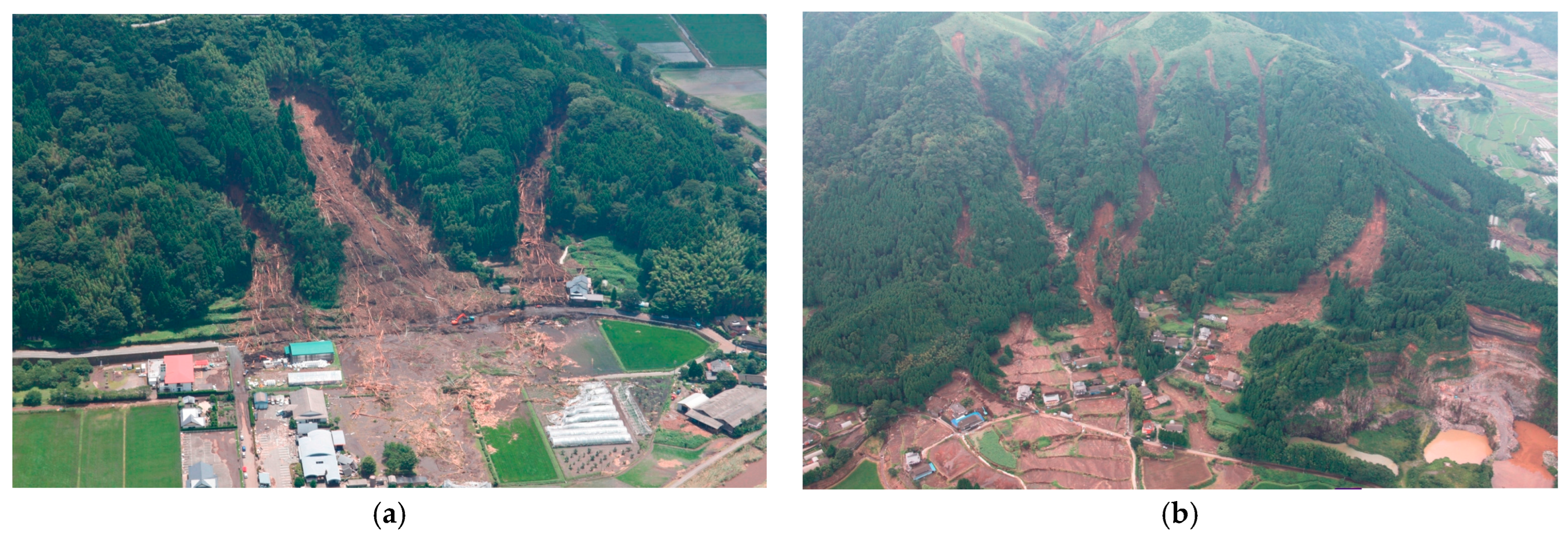
During the rain disaster in northern Kyushu from 11 to 14 July 2012, heavy rainfall exceeding 100 mm/h and 800 mm/24 h was observed mainly in the Kumamoto, Oita, and Fukuoka prefectures (Figure 2). Although rainfall around the Aso caldera area was minor on the 11th, it gradually intensified after midnight on the 12th. Between 2 and 3 a.m., an hourly rainfall of 108.0 mm was observed, with heavy rain continuing until about 6 a.m., measuring between 87 and 96 mm per hour. After that, the rain gradually subsided and had mostly ceased by around 9 a.m. Furthermore, this heavy rain caused widespread flooding and landslides (Figure 3), resulting in 25 confirmed deaths and missing persons, out of which 19 individuals were confirmed dead or missing due to the landslides. Among sediment-related disasters, landslides primarily occur around the eastern caldera wall of the Asodani valley on the northern side of the Aso caldera and the vicinity of Aso mountain. It has been reported that the morphology and characteristics of these landslides vary depending on the location [37].

3. Materials and Methods

Shallow landslides occur due to both triggering factors (such as heavy rain or earthquakes) and primary factors (such as slope angle, geology, and vegetation). We extracted information for slopes where shallow landslides occurred and where they did not, and collected data on primary factors and triggering factors such as rainfall on these slopes. We divided the collected data into a model-building dataset and a testing dataset, and constructed models using two statistical methods: generalized linear models and random forest models. We quantitatively analyzed the impact of vegetation on the occurrence of shallow landslides (Figure 4).

3.1. Extraction of Shallow Landslides Data and Creation of Slope Units

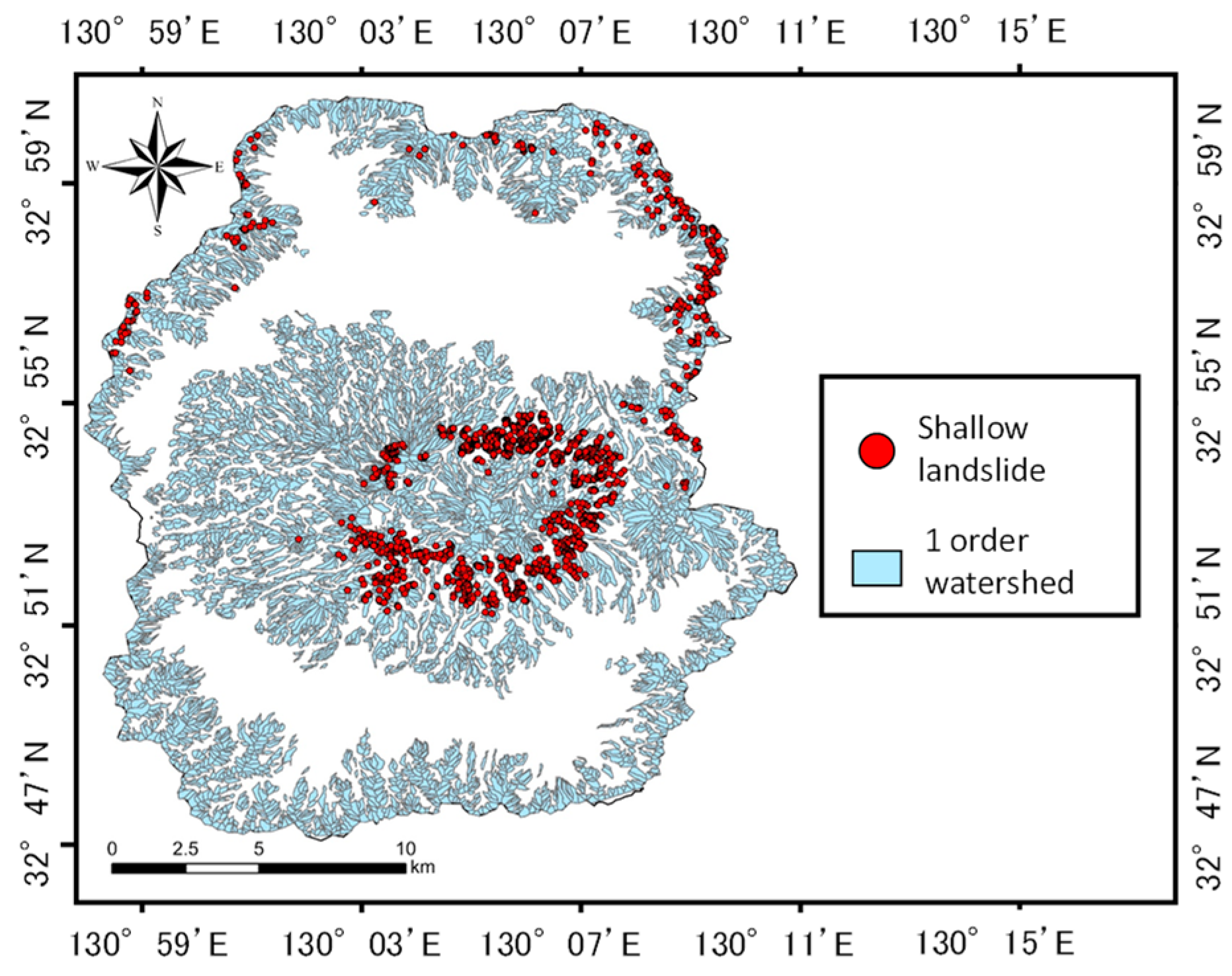
For the interpretation of landslide locations, we used the “Distribution Map of Sediment Movement Associated with the Heavy Rainfall in Northern Kyushu in July 2012” by the Disaster Prevention Research Institute [38]. In this study, we referred to the method by Asada et al. [39] for the interpretation of landslides and the extraction of shallow landslide data. First, a digital elevation model (DEM) based on laser profile (LP) data before and after the disaster was used. The difference in DEM values between before and after the disaster was calculated. The LP data before the disaster were acquired in 2010, while LP data after the disaster were acquired in 2013. The resolution of both DEMs is 1 m. Using the calculated difference values and aerial photographs, 2038 landslides were identified. Next, using the DEM before the disaster, the 1 order watershed areas were created using the hydrological analysis tools of ArcGIS spatial analyst. Finally, landslides within the 1 order watershed areas with an average depth of less than 2 m were defined as shallow landslides [39]. A total of 1347 shallow landslide areas were identified within the 1 order watershed areas. As a result, out of the 2038 landslides interpreted, the data of 1347 shallow landslides were extracted (Figure 5).
For the unit of statistical analysis, we created slope units (SUs) based on the method by Asada et al. [39]. SU represents the area enclosed by ridge lines and valley lines. The ridge lines and valley lines were created using the hydrological analysis tools of ArcGIS spatial analyst. In order to determine the presence or absence of shallow landslide occurrence for each SU dataset, we overlaid the shallow landslide sites and the SU data. The SU that included shallow landslides were designated as landslide SU, and those that did not include shallow landslides were designated as non-landslide SU. However, SU containing landslides that were not shallow landslides were excluded from the analysis.

3.2. Creating Data on Primary Factors for Shallow Landslides

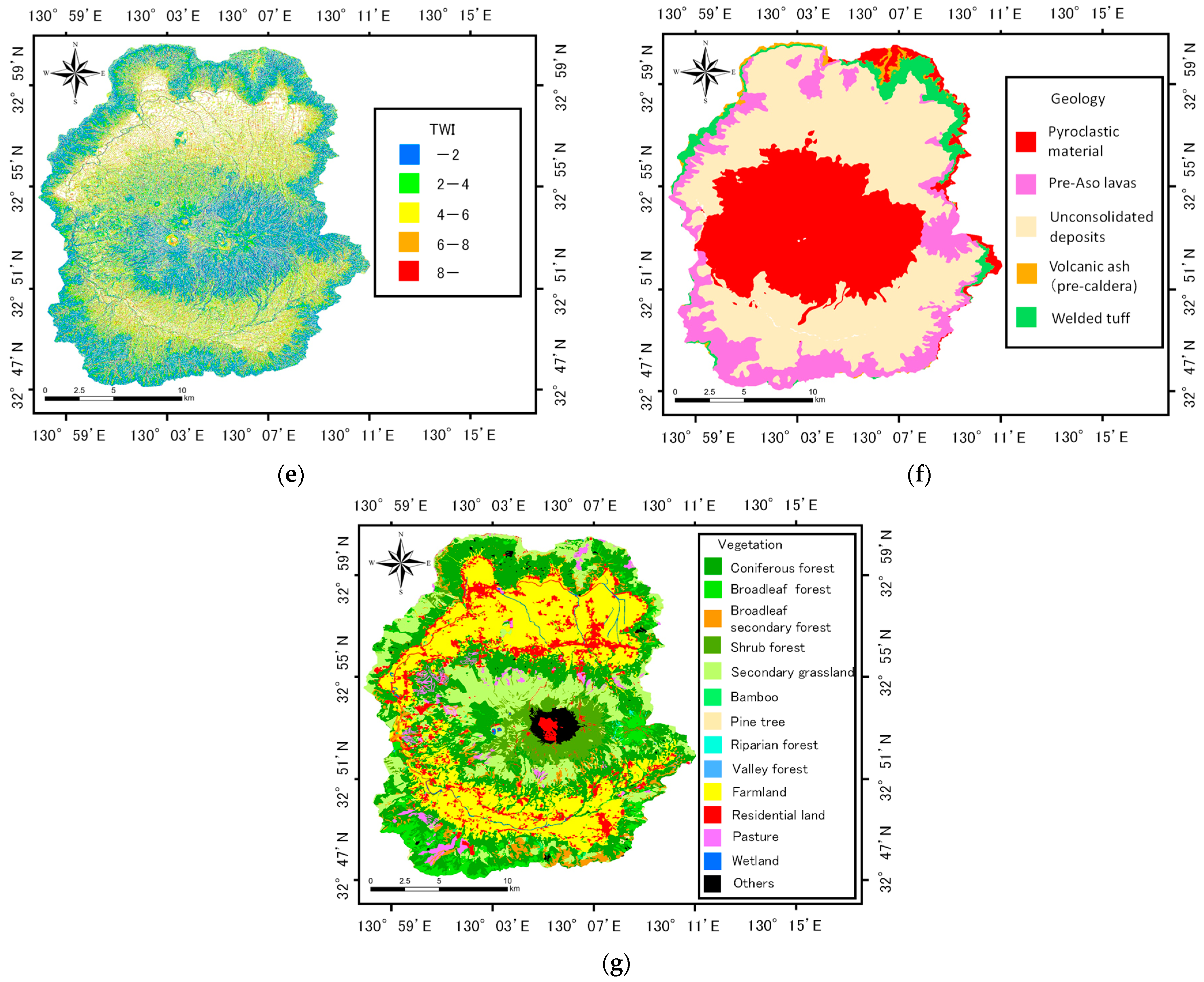
The inherent factors that affect the occurrence of shallow landslides have been shown in previous studies to be elevation [40], slope angle [41], slope aspect [42], undulation [43], SPI (stream power index) [44,45], TWI (topographic wetness index) [44,45], curvature [46], soil thickness [47], surface geology [48], vegetation [3,4,5], landslide history [49], and forest roads [50]. In this study, we decided to analyze elevation, slope, aspect, undulation, surface geology, and vegetation as primary factors (Figure 6). The following paragraphs explain how we created the primary factor data.
Elevation is a parameter that has a significant impact on the occurrence of shallow landslides because it affects many conditions related to the stability of slopes, such as climatic conditions such as temperature, the growth limit of vegetation, and restrictions on human activity areas. We used a 10 m low-resolution DEM (10mDEM) based on pre-disaster LP data. Then, we overlaid the elevation raster data with SU data, calculated the average elevation for each SU dataset, and used this for the analysis.
Slope angle is the most critical parameter concerning the stability of a slope [41]. Slope angle determines the flow of water on the slope, affecting the soil moisture content and the stability of the slope. We created raster data of the slope angle for each mesh using the 10mDEM. Then, we overlaid the raster data of the slope angle with SU data, calculated the average slope angle for each SU dataset, and used this for the analysis.
Slope aspect is a parameter that affects the distribution of shallow landslides because it is related to the amount of solar radiation and humidity [42]. In this study, we created raster data of the slope aspect for each mesh using the 10mDEM. Then, we overlaid the slope aspect raster data with SU data, calculated the average slope aspect for each SU dataset, and used this for the analysis. Slope aspect raster data are expressed in degrees, with north as 0 degrees. We reclassified the aspect into eight compass points (north for 0 to less than 22.5 degrees, northeast for 22.5 to less than 67.5 degrees, east for 67.5 to less than 112.5 degrees, southeast for 112.5 to less than 157.5 degrees, south for 157.5 to less than 202.5 degrees, southwest for 202.5 to less than 247.5 degrees, west for 247.5 to less than 292.5 degrees, northwest for 292.5 to less than 337.5 degrees, and north for 337.5 to 360 degrees).
Undulation is an indicator of the size of a slope, and it has been reported that the proportion of landslide occurrence significantly increases as the undulation increases [43]. In this study, we used the difference between the minimum and maximum altitudes of SU as the undulation.
SPI represents the ease of sediment erosion and TWI represents the potential accumulation of groundwater [51], both of which are essential explanatory variables in assessing the risk of shallow landslides [44,45]. SPI and TWI are defined by the following formulas [51]:
S P I = A s tan β
T W I = l n ( A s / tan β )
where As is the catchment area (m2) and β is the slope angle (rad). Using this equation, SPI and TWI were calculated for each mesh. Then, the raster data of SPI and TWI were overlaid with SU data, and the average values of SPI and TWI for each SU dataset were calculated and used for analysis.
Surface geology (hereinafter referred to as geology) is an indicator that is deeply related to the strength of slopes. Safaei et al. [48] reported that geological divisions of the Paleogene and Neogene were important parameters for the occurrence of shallow landslides compared to other geological divisions. For the creation of geological data, we referred to the Aso Volcanic Geological Map published by the Industrial Research Institute [52]. The volcanic activity of Aso is divided into three periods: the pre-caldera volcanic activity period before the formation of the caldera, the caldera formation period with repeated caldera eruptions, and the post-caldera activity period after the formation of the caldera [53]. Each period’s ejecta is considered to have different geological and petrological characteristics [54]. The ejecta from the pre-caldera activity period is called pre-Aso volcanic lavas [54], mainly composed of biotite rhyolite, pyroxene andesite, and basalt [55]. The ejecta from the caldera formation period is caused by four pyroclastic flows, and mainly consists of non-welded volcanic ash and welded tuff [55]. In the post-caldera activity period, various magma from basalt to rhyolite erupted, forming the central cone group. In the volcanic geological map, the geology of the central cone group is classified into tuff, scoria, volcanic ash, pumice, etc. [55]. In addition, it has been revealed that the surface of the central cone group is volcanic ash and soil layers deposited by volcanic activity over the past 3000 years [56]. From these findings, in this study, the geological classification was divided into five categories: pre-Aso volcanic lavas, welded tuff, volcanic ash deposited at the time of caldera formation (pre-caldera), pyroclastic material including volcanic ash and pumice, and unconsolidated deposits composed of sand and silt. We overlaid the raster data of the divided geology with SU data and used the geological item with the largest area within the SU as the dominant geological item for analysis.
The creation of vegetation data used the Basic GIS Data for Nature Conservation published by the Nature Conservation Bureau of the Ministry of the Environment [57]. Taking into account factors such as tree species, communities, and the condition of root systems, the vegetation data were classified into 13 categories: coniferous forest, broadleaf forest, broadleaf secondary forest, pine tree, valley forest, riparian forest, shrub forest, bamboo, secondary grassland, farmland, pasture, residential land, wetland, and others. The raster data of the vegetation and SU data were overlaid, and the vegetation item with the largest area within the SU was used for analysis.
In addition to the above primary factors, curvature affects the acceleration and deceleration, convergence, and divergence of water flow on the slope surface, which can influence shallow landslides [46], and could also be an indicator of topographic features such as ridges and valleys. However, the SU set as the analysis units in this study is expressed as an area enclosed by ridge lines and valley lines, and it was considered inappropriate to discuss topographic characteristics for each SU dataset using curvature. Therefore, curvature was excluded from the primary factors. Soil thickness is an important parameter for physically discussing the occurrence of shallow landslides, but there was no information to quantitatively show the soil thickness of the entire target area, so soil thickness was excluded from the primary factors. Although the history of landslides could be an indicator when considering the potential susceptibility of a slope to landslides, we could not obtain detailed information on the history of landslides in the area targeted in this study, so we excluded it from the primary factors. Regarding forest roads, it has been pointed out that forest roads can cause shallow landslides by changing the flow of groundwater and increasing the pore water pressure on the slope above the forest road [58]. However, in the area targeted for analysis in this study, there were few forest roads, so we excluded them from the primary factors.

3.3. Creating Data on Triggering Factors for Shallow Landslides

The relationship between rainfall and shallow landslides has been discussed in many previous studies. For example, Dai et al. [58] suggested that 12-h rainfall is the most important factor in predicting the number of landslides. Effective rainfall is also one of the indicators to evaluate the relationship between rainfall and landslides. Yong Hong [59] has shown that the occurrence of landslides actually correlates with effective rainfall. The effective rainfall can be calculated by the following formula [60]:
R w = i α i · R 1 i
α i = 0.5 1 / T
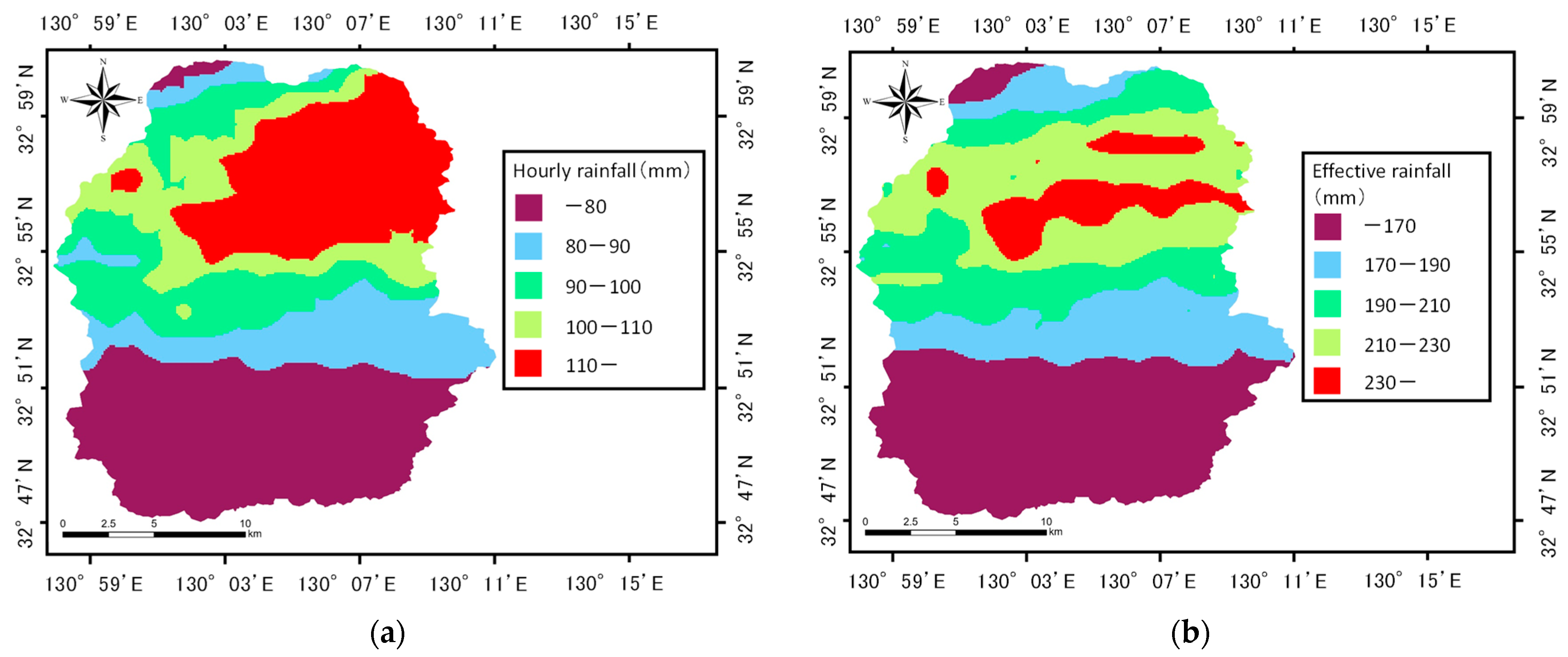
where R w is the effective rainfall at time t, R 1 i is the hourly rainfall i hours ago, α i is the reduction coefficient i hours ago, and T represents the half-life. A 72-h half-life is used for the long-term effective rainfall to represent the long-term impact of rainfall, and a 1.5-h half-life is used for the short-term effective rainfall to represent the short-term impact of rainfall [61]. Additionally, Brand et al. [62] reported that most of the landslides that occurred in Hong Kong were caused by local short-term heavy rain, indicating a strong correlation between the short-term impact of rainfall and the occurrence of landslides. Therefore, in this study, the maximum one-hour rainfall (hereinafter referred to as hourly rainfall), which represents the short-term impact of rainfall, and the short-term effective rainfall (hereinafter referred to as effective rainfall) were adopted as explanatory variables for the trigger (Figure 7). The meteorological variables related to rainfall mentioned above were created using the 1 km mesh analyzed rainfall provided by the Japan Meteorological Agency [63]. The analyzed rainfall is an estimate of the amount of precipitation corrected by the observation values of meteorological radars using rain gauge observation values on an hourly basis. The analyzed rainfall considered was from 0:00 to 10:00 on July 12. The maximum one-hour rainfall and the effective rainfall were created as raster data using the interpolation tools of the ArcGIS spatial analyst, and an overlay was made with the SU data to calculate the maximum value for each SU dataset for analysis. The mesh size for the interpolation was set at 10 m (Table 1).

3.4. Statistical Analysis

3.4.1. Preparation of Model Building Dataset and Testing Dataset

In this study, 70% of the dataset was used for model construction (63,542 data points), and the remaining 30% was used for the test data (27,234 data points) [65,66,67]. When constructing our model, we performed cross-validation. In k-fold cross-validation, the entire dataset is divided into k parts, after which, k − 1 parts are used as training data, and the remaining part is used as validation data. This process is repeated k times. In this study, we performed cross-validation by setting k to 10, referring to previous research [66,68].
Since the dataset used in this study involved highly imbalanced data with a significant number of non-landslide SU data compared to landslide SU data, we used stratified k-fold cross-validation, which divides the data so that the ratio of landslide SU data to non-landslide SU data is the same within the divided range.

3.4.2. Multicollinearity

The variance inflation factor (VIF) can be used to detect a one-to-many correlation; thus, it was adopted as an indicator to confirm the multicollinearity of this analysis. The VIF was calculated with the following formula:
V I F = 1 / ( 1 R 2 )
R is the multiple correlation coefficient.
Generally, if the VIF ≥ 5, there is a suspicion of multicollinearity [69]. Therefore, in this study, the threshold of the VIF was set to 5. When there are values exceeding the threshold, the factor was excluded, and the calculation of the VIF was repeated until all of the factors were less than 5. The R’s car package was used to calculate the VIF.

3.4.3. Generalized Linear Model

The generalized linear model (GLM) can numerically express the relationship between the response variable and explanatory variables and has the feature that it can incorporate explanatory variables of non-normal distributions as well as normal distributions into the model [70]. The probability distribution of the GLM was binomial, and the link function was logit (logistic regression). Logistic regression is one of the most widely used methods for predictive assessment of shallow landslides [20,40]. Logistic regression is represented by the following equation:
P = 1 1 + e ( a + b 1 X 1 + b 2 X 2 + + b n X n ) = e a + b 1 X 1 + b 2 X 2 + + b n X n 1 + e a + b 1 X 1 + b 2 X 2 + + b n X n
where P is the landslide probability, a is the intercept, b 1 , b 2 b n are the regression coefficients corresponding to the explanatory variables X 1 , X 2 X n .
Odds represent the ratio of the probability P (when the response variable is 1) to the probability 1 P (when the response variable is 0). The natural logarithm of odds (logit) is represented by the following equation:
l o g i t P = l n P 1 P = a + b 1 X 1 + b 2 X 2 + + b n X n
In logistic regression, the response variable was set as binary data indicating the presence or absence of landslide occurrence within the SU (landslide: 1, no landslide: 0). The explanatory variables used were elevation, slope angle, slope aspect, SPI, TWI, geology, vegetation, hourly rainfall, and effective rainfall. Categorical variables such as slope aspect were referenced to the north, while geology and vegetation were anchored to the areas with the largest distribution, specifically pyroclastic material and coniferous forests, respectively. To determine the most suitable combination of explanatory variables, the Akaike information criterion (AIC) was used as a reference. The combination of explanatory variables that resulted in the lowest AIC value, indicating the best model fit, was selected.

3.4.4. Random Forest

Random forest (RF) is an ensemble learning method that constructs numerous decision trees and makes a decision based on the majority of these trees, smoothing out the overfitting of decision trees [71]. RF can be used for both classification and regression. In this study, the RF model was constructed as regression. RF employs a technique known as bootstrapping [72] with replacement to create a training dataset by sampling with duplicates allowed. This dataset is then used to generate multiple decision trees. Data that are not selected during this process (out of bag, OOB) are utilized for model accuracy evaluation. Using the constructed model, predictions are made on the OOB data, and the mean squared error (MSE) between the predicted values and actual measurements is computed [73]. The method used to calculate importance was the increase in mean squared error (IncMSE) approach, which estimates how much the MSE increases when making predictions without a particular explanatory variable [71]. RF constructs models with ntree and mtry as the hyperparameters, which were set via cross-validation. ntree represents the number of decision trees to be created, while mtry indicates the number of explanatory variables used when generating decision trees. The response variable and explanatory variables used were the same as those used in the GLM. In addition, other methods such as support vector machines (SVMs) and artificial neural networks (ANNs) have been utilized as predictive assessment techniques for shallow landslides [22,23]. The RF model, which is less susceptible to the effects of overfitting and capable of considering interactions among explanatory variables, was chosen as an analytical method [74]. Moreover, the importance of each explanatory variable, calculated by RF, is visually interpretable, indicating their relative significance. Given these advantages, we chose RF as analytical method.

3.4.5. Model Performance Evaluation

We used the constructed models to predict the test data and evaluated the prediction accuracy of the models. We calculated the accuracy, precision, sensitivity, specificity, and the area under the curve (AUC) as evaluation metrics for the prediction models [66,75]. The accuracy, sensitivity, precision, and specificity were calculated using the following formulas:
A c c u r a c y = T P + T N T P + F P + F N + T N
P r e c i s i o n = T P T P + F P
S e n s i t i v i t y = T P T P + F N
S p e c i f i c i t y = T N T N + F P
True positives (TP), true negatives (TN), false positives (FP), and false negatives (FN) represent the number of data points for the landslide and non-landslide SU (Table 2).
The accuracy indicates the ratio of correctly predicted landslide and non-landslide SU. By calculating the accuracy rate, we can assess the overall predictive precision of the model. The precision shows the ratio of SU that were actually landslides among those predicted to be landslides. By calculating the precision, we can evaluate the accuracy when predicting landslides. The sensitivity represents the ratio of SU correctly predicted as landslides among those that actually experienced landslides. By calculating the sensitivity, we can evaluate whether landslide data can be predicted without overlooking. The specificity indicates the ratio of SU correctly predicted as non-landslides among those that did not experience landslides. By calculating the specificity, we can assess whether non-landslide data can be predicted without overlooking.
The AUC is represented by the area below the receiver operating characteristic (ROC) curve, and is calculated using the following formula [75]:
A U C = ( T P + T N ) ( Y + N )
Y represents the number of landslide SU, and N represents the number of non-landslide SU. If the AUC is 0.7 or higher, then it explains the dependent variable of the model well, whereas if it is below 0.5, then the model is considered to have no explanatory power [76].

4. Results

4.1. Correlation Analysis

The variables that resulted in a VIF ≥ 5 were hourly rainfall and effective rainfall. As these variables are explanatory factors of the same cause, it was considered that they led to a high VIF. Therefore, they were incorporated, one at a time, and the VIF was recalculated. The VIFs for all of the variables became less than 5 (Table 3). For the model construction, hourly rainfall and effective rainfall were incorporated as factors one at a time.

4.2. Generalized Linear Model

The GLM was constructed, and the model with the lowest AIC was selected. This model included the following as intrinsic factors: elevation, slope angle, slope aspect, undulation, TWI, geology, vegetation, and the hourly rainfall as an inducing factor. The AIC was 8048.3. Significant explanatory variables that positively contributed to the landslide were slope angle (z = 11.78, p < 0.01), undulation (z = 9.75, p < 0.01), and hourly rainfall (z = 14.57, p < 0.01). It was found that the eastern and southern directions were more susceptible to landslides than the northern direction, which was set as the reference. Regarding vegetation, secondary grasslands and shrubs were more prone to landslides than coniferous forests, which were set as the reference. On the other hand, elevation (z = −3.52, p < 0.01) and TWI (z = −8.63, p < 0.01) were selected as significant explanatory variables that negatively contributed to landslides. The results showed that the volcanic ash (pre-caldera), pre-Aso lavas, unconsolidated deposits, and welded tuffs were less susceptible to landslides than the volcanic debris, which was set as the reference. Regarding vegetation, the secondary broadleaf forests, residential land and others were less prone to landslides than coniferous forests, which were set as the reference (Table 4). Multiple comparison tests for the regression coefficients of the categorical variable, vegetation, revealed significant differences between multiple categories (Appendix A). To visually understand these differences, the landslide probability for each category in the vegetation derived from the GLM and the results of the multiple comparison test are shown in Figure 8. Secondary grassland and shrubs had significantly higher landslide probabilities compared to coniferous forests, broadleaf forests, secondary broadleaf, residential land and others, exceeding the cut-off value. The landslide probability of secondary grassland was approximately three times higher compared to coniferous and broadleaf forests and approximately nine times higher compared to broadleaf secondary forests. Similarly, the landslide probability of shrubs was approximately four times higher compared to coniferous, and broadleaf forests, and approximately ten times higher compared to broadleaf secondary forests. No significant differences were detected between coniferous and broadleaf forests and broad- leaf secondary forests.
A stratified 10-fold cross-validation was performed and the AUC values for the validation data were calculated (Table 5). The median AUC was 0.91.
Predictions were made for the test data using the constructed model. The accuracy was 0.84, the precision was 0.08, the sensitivity was 0.83, the specificity was 0.84, and the AUC was 0.91 (Table 6). Despite low precision, a model with excellent predictive accuracy was constructed. The model’s cut-off value was 0.026.

4.3. Random Forest

The hyperparameters for the RF model were determined using stratified 10-fold cross-validation, with ntree = 5000 and mtry = 3. Thus, a model was constructed with ntree = 5000 and mtry = 3, and the importance was calculated (Figure 9). Hourly rainfall had the highest importance, followed by geology, then elevation.
A stratified 10-fold cross-validation was performed and the AUC for the validation data was calculated (Table 7). The median AUC was 0.95.
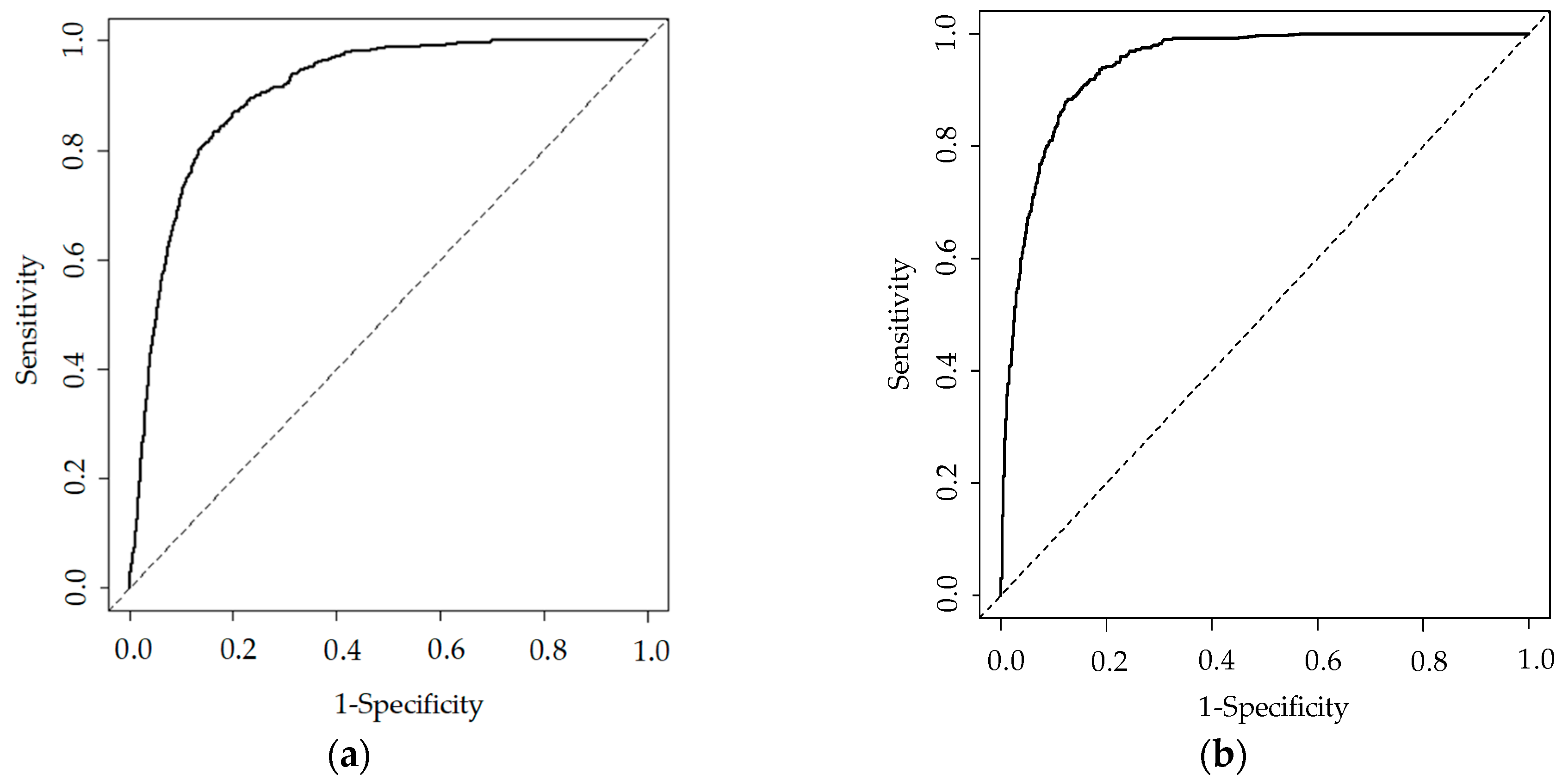
Predictions were made for the test data using the constructed model. The accuracy was 0.87, the precision was 0.11, the sensitivity was 0.88, the specificity was 0.87, and the AUC was 0.95 (Table 8, Figure 10). Despite low precision, a model with good accuracy was constructed. The model’s cut-off value was 0.029.

5. Discussion

5.1. Model Performance Evaluation

The AUC of the constructed model was higher for the RF model than the GLM. In many previous studies related to the prediction and assessment of shallow landslides, these have also shown that the RF model is more accurate than the GLM [73,77]. In this study, the precision was low for both models. This is thought to be due to the fact that the amount of landslide SU data is extremely small compared to the non-landslide SU data. Methods used to overcome imbalanced data include oversampling by SMOTE (synthetic minority over-sampling technique) [78], and it is thought that using such methods could improve the accuracy of the model. However, the low precision indicates that while there is a possibility of misclassification, there are few missed landslide locations, suggesting a model that evaluates on the safe side for disaster prevention. Therefore, it is not considered a problem in evaluating the impact of vegetation on shallow landslides.

5.2. Impact of Vegetation on Shallow Landslides

Based on the results of the GLM, it became clear that the landslide probability of secondary grassland is higher than that of forests, such as coniferous forests. Previous studies have not evaluated the difference in vegetation and have not discussed the extent of the difference in landslide probability due to the difference in vegetation [24,25]. By showing landslide probabilities for each type of vegetation, it is expected to provide useful insights for considering appropriate vegetation management in the Aso region. As a factor for the forest having a lower probability than grasslands, the difference in the root mass and distribution between forests and grasslands can be considered. Using analytical methods based on physical models, it is pointed out that forests have a more significant impact on slope stability than grasslands [34]. Forests, in addition to the mechanical effects of their root systems [4,5], also capture and block rainfall through their canopies, increasing the amount of evapotranspiration. Therefore, forests reduce the amount of water that infiltrates the soil, leading to increased slope stability [79,80]. Due to these effects, we consider that the landslide probability in forests is lower compared to grasslands. However, determining which of the effects brought by the forest dominated in influencing slope stability is difficult using statistical methods. In the future, it is essential to evaluate which function of the forest was dominant using analytical methods based on physical models.
Furthermore, slope angle and hourly rainfall are important parameters in evaluating slope stability. Therefore, using the model created with the GLM, response curves of the slope and hourly rainfall for grassland and coniferous forest were created (Figure 11). Grasslands exceeded the cutoff value for slope angle at approximately 25 degrees. In contrast, forests exceeded the cutoff value for slope angle at approximately 45 degrees. Although the influence of root diameter and distribution on slope stability is not uniform [81], even on steep slopes, it was clear that forests increase slope stability more than grasslands. Grasslands exceeded the cutoff value at an hourly rainfall of around 80 mm, while coniferous forests exceeded the cutoff value at an hourly rainfall of around 110 mm. Both forests and grasslands have functions that increase slope stability regardless of the state of soil moisture in the slope [6], but it has become quantitatively clear that forests increase slope stability to a certain extent compared to grasslands. However, the ability of forest to stabilize slopes is limited [6], so it should be noted that the forest does not suppress all cases of shallow landslides. Moreover, it has been pointed out that the spatial structure of forests has a significant impact on slope stability. It has been shown that when gaps within the forest exceed 20 m, susceptibility to landslides increases [26]. Therefore, it is important to conduct analyses that consider detailed information about forests in the future. On the other hand, for grasslands, it is said that the stabilizing effect on slopes varies depending on the type of herbaceous plant present [28,29], but it has been pointed out that the research on such stabilizing effect on slopes is insufficient compared to that for forests [82]. In the future, it will be necessary to accumulate knowledge using statistical methods as in this study and to mechanically grasp the slope stabilization effect that grasslands have using analytical methods. In addition, it has been reported that grasslands have smaller landslide depth and sediment production than forests [35]. Grasslands and forests differ significantly in their above-ground biomass. In forested areas, shallow landslides can result in a large number of fallen trees, potentially providing driftwood to rivers, as pointed out in [83]. Consequently, the impact on downstream areas is presumed to be lesser from forests compared to grasslands. The soil-strengthening effects of forest root systems are believed to influence not only the landslide probability but also the scale of these landslides [26]. Therefore, future assessments should focus not only on the likelihood of landslides but also on their scale when evaluating the risks associated with forests and grasslands.

5.3. Importance of Contributing Factors

The importance calculated by the RF model was highest for hourly rainfall, followed by geology, then elevation. The specific disaster targeted in this study was heavy rain exceeding 100 mm of hourly rainfall, and the influence of the inducement was very large, so it was conjectured that the importance became large. Geology showed an importance that was equivalent to maximum hourly rainfall. The shallow landslides that occurred in the target area occurred in large numbers in volcanic ash layer geology [37]. Since the volcanic ash layer is extremely permeable, it has been pointed out that landslides are likely to occur at boundaries with less permeable layers [84]. Therefore, it was considered that the importance of geology, which is closely related to rainfall, became high. In previous studies, it has also been shown that geology such as volcanic ash has made a major contribution to the occurrence of shallow landslides [85]. The elevation showed a significant importance next to the maximum hourly rainfall and geology. Elevation, which greatly influences the growth limit of vegetation and constrains human activity areas, has also been shown to have a high importance [77]. The importance of vegetation was smaller than that of rainfall and geology. In previous research, vegetation had about 40% of the importance compared to rainfall [39], and this study showed the same trend. However, even if the importance is small, as shown in Figure 9, under limited conditions, it is considered that vegetation functions to suppress shallow landslides. Additionally, with statistical methods, it is not possible to assess the impact on slope collapses from variables that could not be incorporated into the model (for instance, soil layer thickness). Moving forward, it is essential to gather data on variables not addressed in this study and integrate them into the model.

6. Conclusions

In this study, we aimed to quantitatively assess the impact of different vegetation conditions, such as grasslands and forests, on the occurrence of shallow landslides using statistical methods. We constructed the GLM and the RF models. The model that resulted in the lowest AIC in the GLM included elevation, slope angle, slope aspect, undulation, TWI, geology, and vegetation as primary factors, and the hourly rainfall as a trigger factor. Slope angle, undulation, and hourly rainfall were selected as significant explanatory variables that contribute positively to shallow landslides. On the other hand, elevation and TWI were selected as significant explanatory variables that contribute negatively to shallow landslides. Significant differences were observed among multiple categories of vegetation. The probability of shallow landslides in secondary grasslands was approximately three times that of coniferous and broadleaf forests, and approximately nine times that of broadleaf secondary forests. The landslide probability of shrubs was approximately four times that of coniferous and broadleaf forests, and approximately ten times that of broadleaf secondary forests. The results of constructing the RF model showed that the importance was highest for the hourly rainfall, followed by geology, then elevation. AUC values for the GLM and the RF model were 0.91 and 0.95, respectively, indicating that highly accurate models were constructed. This study quantitatively demonstrated the impact of vegetation differences on shallow landslides. The insights gained from this study will be essential for considering appropriate vegetation management to reduce the risk of future shallow landslides. However, while this study discussed the probability of shallow landslide occurrence, it is important to note that landslide risk involves not only probabilities but also factors such as the scale of landslides and their downstream impacts, including the supply of sediment and debris. Therefore, future research should analyze the influence of vegetation on the scale of shallow landslides and their downstream effects.

Author Contributions

Conceptualization, H.A. and T.M.; software, H.A.; methodology, H.A.; validation, H.A. and T.M.; formal analysis, H.A.; investigation, H.A. and T.M.; resources, H.A.; writing—original draft preparation, H.A.; writing—review and editing, H.A. and T.M.; supervision, T.M.; project administration, T.M.; funding acquisition, T.M. All authors have read and agreed to the published version of the manuscript.

Funding

This study was supported by the Environmental Research and Technology Development Fund of the Environmental Restoration and Conservation Agency of Japan (Grant Numbers: JPMEERF19S20530, JPMEERF20234005), and the Collaborative Creation Support Program of the Japan Science and Technology Agency (Grant Number: JPMJPF2109).

Data Availability Statement

Not applicable.

Acknowledgments

The authors would like to sincerely acknowledge the editors and anonymous reviewers for their expert comments and suggestions on this manuscript.

Conflicts of Interest

The authors declare no conflict of interest.

Appendix A

Summary of the multiple comparison test for vegetation. The upper triangular matrix represents the estimated difference of the regression coefficients and the lower triangular matrix represents the standard error. The sign of the estimate indicates a positive value when the coefficient value of the column category is higher than the coefficient value of the row category. Bold numbers indicate estimates where the p value was less than 0.05.
Table A1. Summary of the multiple comparison test for vegetation (From Coniferous Forest to Pasture).
FactorsConiferous ForestBambooBroadleaf ForestBroadleaf Secondary ForestFarmlandOthersPasture
Coniferous forest-−13.08−0.090.94−12.47−0.95−0.87
Bamboo671.3-12.9912.140.6012.1312.21
Broadleaf
forest
0.26671.3-−0.85141−0.86−0.78
Broadleaf
secondary
forest
0.35671.30.42-141−0.010.07
Farmland14168612.3811.53-11.5311.61
Others0.37671.30.430.49141-0.08
Pasture0.72671.30.760.791410.79-
Pine tree1.02671.31.041.071411.071.24
Residential land0.59671.30.630.681410.670.92
Riparian forest125814261258.001258.0012661258.001258.00
Secondary grassland0.11671.30.250.351410.350.71
Shrub
forest
0.13671.30.260.351410.340.72
Valley forest1829194818291829183418291829
Wetland2229232822292229223322292229
Table A2. Summary of the multiple comparison test for vegetation (From Pine tree to Wetland).
FactorsPine
Tree
Residential LandRiparian
Forest
Secondary
Grassland
Shrub
Forest
Valley
Forest
Wetland
Coniferous forest−0.04−1.54−13.281.261.37−14.34−12.36
Bamboo13.0411.54−0.2014.3314.45−1.270.72
Broadleaf
forest
0.05−1.45−13.191.341.46−14.25−12.27
Broadleaf
secondary
forest
0.90−0.60−12.342.202.31−13.4−11.42
Farmland12.4410.93−0.8013.7313.84−1.870.11
Others0.91−0.59−12.332.202.32−13.4−11.41
Pasture0.83−0.67−12.412.122.24−13.48−11.49
Pine tree-−1.50−13.241.291.41−14.31−12.32
Residential land1.17-−11.742.802.91−12.80−10.82
Riparian
forest
1258.001258.00-14.5314.65−1.070.92
Secondary grassland1.010.581258-0.11−15.6−13.61
Shrub
forest
1.020.5812580.09-−15.71−13.73
Valley forest18291829222018291829-1.98
Wetland222922292559222922292883-

References

  1. Murgia, I.; Giadrossich, F.; Mao, Z.; Cohen, D.; Capra, G.F.; Schwarz, M. Modeling shallow landslides and root reinforcement: A review. Ecol. Eng. 2022, 181, 106671. [Google Scholar] [CrossRef]
  2. Ran, Q.; Hong, Y.; Li, W.; Gao, J. A modelling study of rainfall-induced shallow landslide mechanisms under different rainfall characteristics. J. Hydrol. 2018, 563, 790–801. [Google Scholar] [CrossRef]
  3. Persichillo, M.G.; Bordoni, M.; Meisina, C. The role of land use changes in the distribution of shallow landslides. Sci. Total Environ. 2017, 574, 924–937. [Google Scholar] [CrossRef] [PubMed]
  4. Cohen, D.; Schwarz, M. Tree-root control of shallow landslides. Earth Surf. Dyn. 2017, 5, 451–477. [Google Scholar] [CrossRef]
  5. Schwarz, M.; Cohen, D.; Or, D. Pullout tests of root analogs and natural root bundles in soil: Experiments and modeling. J. Geophys. Res. Atmos. 2011, 116, F02007. [Google Scholar] [CrossRef]
  6. Liu, C.; Bi, H.; Wang, D.; Li, X. Stability Reinforcement of Slopes Using Vegetation Considering the Existence of Soft Rock. Appl. Sci. 2021, 11, 9228. [Google Scholar] [CrossRef]
  7. Getzner, M.; Gutheil-Knopp-Kirchwald, G.; Kreimer, E.; Kirchmeir, H.; Huber, M. Gravitational natural hazards: Valuing the protective function of Alpine forests. For. Policy Econ. 2017, 80, 150–159. [Google Scholar] [CrossRef]
  8. Montgomery, D.R.; Dietrich, W.E. A physically based model for the topographic control on shallow landsliding. Water Resour. Res. 1994, 30, 1153–1171. [Google Scholar] [CrossRef]
  9. Wu, W.; Sidle, R.C. A distributed slope stability model for steep forested basins. Water Resour. Res. 1995, 31, 2097–2110. [Google Scholar] [CrossRef]
  10. Schwarz, M.; Cohen, D.; Or, D. Spatial characterization of root reinforcement at stand scale: Theory and case study. Geomorphology 2012, 171–172, 190–200. [Google Scholar] [CrossRef]
  11. Mao, Z.; Jourdan, C.; Bonis, M.-L.; Pailler, F.; Rey, H.; Saint-André, L.; Stokes, A. Modelling root demography in heterogeneous mountain forests and applications for slope stability analysis. Plant Soil 2012, 363, 357–382. [Google Scholar] [CrossRef]
  12. Schwarz, M.; Lehmann, P.; Or, D. Quantifying lateral root reinforcement in steep slopes—From a bundle of roots to tree stands. Earth Surf. Process. Landf. 2010, 35, 354–367. [Google Scholar] [CrossRef]
  13. Giadrossich, F.; Schwarz, M.; Marden, M.; Marrosu, R.; Phillips, C. Minimum representative root distribution sampling for calculating slope stability in Pinus radiata D.Don plantations in New Zealand. N. Z. J. For. Sci. 2020, 50, 5. [Google Scholar] [CrossRef]
  14. Schwarz, M.; Cohen, D.; Or, D. Root-soil mechanical interactions during pullout and failure of root bundles. J. Geophys. Res. Atmos. 2010, 115, F04035. [Google Scholar] [CrossRef]
  15. Gehring, E.; Conedera, M.; Maringer, J.; Giadrossich, F.; Guastini, E.; Schwarz, M. Shallow landslide disposition in burnt European beech (Fagus sylvatica L.) forests. Sci. Rep. 2019, 9, 8638. [Google Scholar] [CrossRef] [PubMed]
  16. Vergani, C.; Schwarz, M.; Soldati, M.; Corda, A.; Giadrossich, F.; Chiaradia, E.A.; Morando, P.; Bassanelli, C. Root reinforcement dynamics in subalpine spruce forests following timber harvest: A case study in Canton Schwyz, Switzerland. CATENA 2016, 143, 275–288. [Google Scholar] [CrossRef]
  17. Giadrossich, F.; Cohen, D.; Schwarz, M.; Seddaiu, G.; Contran, N.; Lubino, M.; Valdés-Rodríguez, O.A.; Niedda, M. Modeling bio-engineering traits of Jatropha curcas L. Ecol. Eng. 2016, 89, 40–48. [Google Scholar] [CrossRef]
  18. Merghadi, A.; Yunus, A.P.; Dou, J.; Whiteley, J.; ThaiPham, B.; Bui, D.T.; Avtar, R.; Abderrahmane, B. Machine learning methods for landslide susceptibility studies: A comparative overview of algorithm performance. Earth Sci. Rev. 2020, 207, 103225. [Google Scholar] [CrossRef]
  19. Guzzetti, F.; Reichenbach, P.; Ardizzone, F.; Cardinali, M.; Galli, M. Estimating the quality of landslide susceptibility models. Geomorphology 2006, 81, 166–184. [Google Scholar] [CrossRef]
  20. Abeysiriwardana, H.D.; Gomes, P.I.A. Integrating vegetation indices and geo-environmental factors in GIS-based landslide-susceptibility mapping: Using logistic regression. J. Mt. Sci. 2022, 19, 477–492. [Google Scholar] [CrossRef]
  21. Sun, X.; Chen, J.; Han, X.; Bao, Y.; Zhan, J.; Peng, W. Application of a GIS-based slope unit method for landslide susceptibility mapping along the rapidly uplifting section of the upper Jinsha River, South-Western China. Bull. Eng. Geol. Environ. 2019, 79, 533–549. [Google Scholar] [CrossRef]
  22. Zhao, P.; Masoumi, Z.; Kalantari, M.; Aflaki, M.; Mansourian, A. A GIS-Based Landslide Susceptibility Mapping and Variable Importance Analysis Using Artificial Intelligent Training-Based Methods. Remote Sens. 2022, 14, 211. [Google Scholar] [CrossRef]
  23. Zhao, Z.; Liu, Z.Y.; Xu, C. Slope Unit-Based Landslide Susceptibility Mapping Using Certainty Factor, Support Vector Machine, Random Forest, CF-SVM and CF-RF Models. Front. Earth Sci. 2021, 9, 589630. [Google Scholar] [CrossRef]
  24. Nandi, A.; Shakoor, A. A GIS-based landslide susceptibility evaluation using bivariate and multivariate statistical analyses. Eng. Geol. 2010, 110, 11–20. [Google Scholar] [CrossRef]
  25. Neuhäuser, B.; Damm, B.; Terhorst, B. GIS-based assessment of landslide susceptibility on the base of the Weights-of-Evidence model. Landslides 2011, 9, 511–528. [Google Scholar] [CrossRef]
  26. Moos, C.; Bebi, P.; Graf, F.; Mattli, J.; Rickli, C.; Schwarz, M. How does forest structure affect root reinforcement and susceptibility to shallow landslides? Earth Surf. Process. Landf. 2015, 41, 951–960. [Google Scholar] [CrossRef]
  27. Zhang, Y.; Shen, C.; Zhou, S.; Luo, X. Analysis of the Influence of Forests on Landslides in the Bijie Area of Guizhou. Forests 2022, 13, 1136. [Google Scholar] [CrossRef]
  28. Teerawattanasuk, C.; Maneecharoen, J.; Bergado, D.T.; Voottipruex, P.; Le, G.L. Root strength measurements of Vetiver and Ruzi grasses. Lowl. Technol. Int. 2014, 16, 71–80. [Google Scholar] [CrossRef] [PubMed]
  29. Hao, G.; Liu, X.; Zhang, Q.; Xiang, L.; Yu, B. Optimum Selection of Soil-Reinforced Herbaceous Plants Considering Plant Growth and Distribution Characteristics. J. Soil Sci. Plant Nutr. 2022, 22, 1743–1757. [Google Scholar] [CrossRef]
  30. Miyabuchi, Y.; Sugiyama, S. 90,000-year phytolith record from tephra section at the northeastern rim of Aso caldera, Japan. Quat. Int. 2011, 246, 239–246. [Google Scholar] [CrossRef]
  31. Miyabuchi, Y.; Sugiyama, S.; Nagaoka, Y. Vegetation and fire history during the last 30,000 years based on phytolith and macroscopic charcoal records in the eastern and western areas of Aso Volcano, Japan. Quat. Int. 2010, 254, 28–35. [Google Scholar] [CrossRef]
  32. Koyama, A.; Koyanagi, T.F.; Akasaka, M.; Takada, M.; Okabe, K. Combined burning and mowing for restoration of abandoned semi-natural grasslands. Appl. Veg. Sci. 2016, 20, 40–49. [Google Scholar] [CrossRef]
  33. Liu, J.; Wu, Z.; Zhang, H. Analysis of Changes in Landslide Susceptibility according to Land Use over 38 Years in Lixian County, China. Sustainability 2021, 13, 10858. [Google Scholar] [CrossRef]
  34. Kokutse, N.K.; Temgoua, A.G.T.; Kavazović, Z. Slope stability and vegetation: Conceptual and numerical investigation of mechanical effects. Ecol. Eng. 2016, 86, 146–153. [Google Scholar] [CrossRef]
  35. Koyanagi, K.; Gomi, T.; Sidle, R.C. Characteristics of landslides in forests and grasslands triggered by the 2016 Kumamoto earthquake. Earth Surf. Process. Landforms 2019, 45, 893–904. [Google Scholar] [CrossRef]
  36. Kamp, U.; Growley, B.J.; Khattak, G.A.; Owen, L.A. GIS-based landslide susceptibility mapping for the 2005 Kashmir earthquake region. Geomorphology 2008, 101, 631–642. [Google Scholar] [CrossRef]
  37. Miyabuchi, Y. Landslides Triggered by the July 2012 Torrential Rain in Aso Caldera, Southwestern Japan. J. Geogr. (Chigaku Zasshi) 2012, 121, 1073–1080. [Google Scholar] [CrossRef]
  38. National Research Institute for Earth Science and Disaster Resilience. Sediment Movement Distribution Map due to the Ku-mamoto Earthquake. Available online: http://www.bosai.go.jp/mizu/dosha.html (accessed on 24 May 2023).
  39. Asada, H.; Minagawa, T.; Koyama, A.; Ichiyanagi, H. Factor analysis of surface collapse on slopes caused by the July 2017 Northern Kyushu Heavy Rain. Ecol. Civ. Eng. 2020, 23, 185–196. [Google Scholar] [CrossRef]
  40. Chen, W.; Sun, Z.; Han, J. Landslide Susceptibility Modeling Using Integrated Ensemble Weights of Evidence with Logistic Regression and Random Forest Models. Appl. Sci. 2019, 9, 171. [Google Scholar] [CrossRef]
  41. Lee, S.; Min, K. Statistical analysis of landslide susceptibility at Yongin, Korea. Environ. Geol. 2001, 40, 1095–1113. [Google Scholar] [CrossRef]
  42. Capitani, M.; Ribolini, A.; Bini, M. The slope aspect: A predisposing factor for landsliding? C. R. Geosci. 2013, 345, 427–438. [Google Scholar] [CrossRef]
  43. Takezawa, N.; Uchida, T.; Ishizuka, T.; Honma, S.; Kobayashi, Y.; Miyajima, M. Assessing of scale and susceptibility of landslides to earthquake focused on slope relief. J. Jpn. Soc. Eros. Control Eng. 2013, 65, 22–29. [Google Scholar]
  44. Pourghasemi, H.R.; Mohammady, M.; Pradhan, B. Landslide susceptibility mapping using index of entropy and conditional probability models in GIS: Safarood Basin, Iran. CATENA 2012, 97, 71–84. [Google Scholar] [CrossRef]
  45. Jaafari, A. LiDAR-supported prediction of slope failures using an integrated ensemble weights-of-evidence and analytical hierarchy process. Environ. Earth Sci. 2018, 77, 42. [Google Scholar] [CrossRef]
  46. Ohlmacher, G.C. Plan curvature and landslide probability in regions dominated by earth flows and earth slides. Eng. Geol. 2007, 91, 117–134. [Google Scholar] [CrossRef]
  47. Uchida, T.; Mori, N.; Tamura, K.; Terada, H.; Takiguchi, S.; Kamee, K. The role of data preparation on shallow landslide pre-diction. Jpn. Soc. Eros. Control Eng. 2009, 62, 23–31. [Google Scholar] [CrossRef]
  48. Safaei, M.; Omar, H.; Huat, B.K.; Yousof, Z.B.M. Relationship between Lithology Factor and landslide occurrence based on Information Value (IV) and Frequency Ratio (FR) approaches—Case study in North of Iran. Electron. J. Geotech. Eng. 2012, 17, 79–90. [Google Scholar]
  49. Oka, N.; Kazama, H.; Akutagawa, S.; Oda, M. Site characteristics of slope failures caused by rainfall. Doboku Gakkai Ronbunshu 1993, 1993, 11–20. [Google Scholar] [CrossRef]
  50. Seyed, A.H.; Reza, L.; Majid, L.; Ataollah, K.; Aidin, P. The effect of terrain factors on landslide features along forest road. Afr. J. Biotechnol. 2011, 10, 14108–14115. [Google Scholar] [CrossRef]
  51. Moore, I.D.; Grayson, R.B.; Ladson, A.R. Digital terrain modelling: A review of hydrological, geomorphological, and biological applications. Hydrol. Processes 1991, 5, 3–30. [Google Scholar] [CrossRef]
  52. National Institute of Advanced Industrial Science and Technology. Geological Map of Aso Volcano. Available online: https://www.gsj.jp/Map/JP/volcano.html (accessed on 24 May 2023).
  53. Furukawa, K.; Miyoshi, M.; Shinmura, T.; Shibata, T.; Arakawa, Y. Geology and petrology of the pre-Aso volcanic rocks distributed in the NW wall of Aso Caldera: Eruption style and magma plumbing system of the pre-caldera volcanism. J. Geol. Soc. Jpn. 2009, 115, 658–671. [Google Scholar] [CrossRef]
  54. Ono, K. Geology of the Eastern Part of Aso Caldera, Central Kyushu, Southwest Japan. J. Geol. Soc. Jpn. 1965, 71, 541–553. [Google Scholar] [CrossRef]
  55. Ono, K.; Watanabe, K. Geological Map of Aso Volcano (1:50,000); Geological Map of Volcanoes 4; Geological Survey of Japan: Tsukuba, Japan, 1985.
  56. Miyabuchi, Y. Post-caldera explosive activity inferred from improved 67–30ka tephrostratigraphy at Aso Volcano, Japan. J. Volcanol. Geotherm. Res. 2011, 205, 94–113. [Google Scholar] [CrossRef]
  57. Ministry of Environment. Natural Environment Survey Web-GIS. Available online: http://gis.biodic.go.jp/webgis/index.html (accessed on 24 May 2023).
  58. Dai, F.; Lee, C. Frequency–volume relation and prediction of rainfall-induced landslides. Eng. Geol. 2001, 59, 253–266. [Google Scholar] [CrossRef]
  59. Hong, Y.; Hiura, H.; Shino, K.; Sassa, K.; Suemine, A.; Fukuoka, H.; Wang, G. The influence of intense rainfall on the activity of large-scale crystalline schist landslides in Shikoku Island, Japan. Landslides 2005, 2, 97–105. [Google Scholar] [CrossRef]
  60. Yano, K. Study of the Method for Setting Standard Rainfall of Debris Flow by the Reform of Antecedent Rain. Jpn. Soc. Eros. Control Eng. 1990, 43, 3–13. [Google Scholar] [CrossRef]
  61. Terada, H.; Nakaya, H. Operating Methods of Critical Rainfall for Warning and Evacuation from Sediment-Related Disasters. Technical Note of National Institute for Land and Infrastructure Management; Ministry of Land, Infrastructure, Transport and Tourism: Tokyo, Japan, 2001; Volume 5, pp. 1–58.
  62. Brand, E.W.; Premchitt, J.; Phillipson, H.B. Relationship between rainfall and landslides in Hong Kong. In Proceedings of the Fourth International Symposium on Landslides, Toronto, ON, Canada, 16–21 September 1984; Volume 1, pp. 377–384. [Google Scholar]
  63. Japan Meteorological Agency: Japan Meteorological Business Support Center. Available online: http://www.jma.go.jp/jma/index.html (accessed on 24 May 2023).
  64. Dutton, A.L.; Loague, K.; Wemple, B.C. Simulated effect of a forest road on near-surface hydrologic response and slope stability. Earth Surf. Process. Landf. 2005, 30, 325–338. [Google Scholar] [CrossRef]
  65. Dou, J.; Bui, D.T.; Yunus, A.P.; Jia, K.; Song, X.; Revhaug, I.; Xia, H.; Zhu, Z. Optimization of Causative Factors for Landslide Susceptibility Evaluation Using Remote Sensing and GIS Data in Parts of Niigata, Japan. PLoS ONE 2015, 10, e0133262. [Google Scholar] [CrossRef]
  66. Wang, Y.; Sun, D.; Wen, H.; Zhang, H.; Zhang, F. Comparison of Random Forest Model and Frequency Ratio Model for Landslide Susceptibility Mapping (LSM) in Yunyang County (Chongqing, China). Int. J. Environ. Res. Public Health 2020, 17, 4206. [Google Scholar] [CrossRef]
  67. Liu, R.; Yang, X.; Xu, C.; Wei, L.; Zeng, X. Comparative Study of Convolutional Neural Network and Conventional Machine Learning Methods for Landslide Susceptibility Mapping. Remote Sens. 2022, 14, 321. [Google Scholar] [CrossRef]
  68. Park, S.; Hamm, S.-Y.; Kim, J. Performance Evaluation of the GIS-Based Data-Mining Techniques Decision Tree, Random Forest, and Rotation Forest for Landslide Susceptibility Modeling. Sustainability 2019, 11, 5659. [Google Scholar] [CrossRef]
  69. Kalantar, B.; Ueda, N.; Saeidi, V.; Ahmadi, K.; Halin, A.A.; Shabani, F. Landslide Susceptibility Mapping: Machine and Ensemble Learning Based on Remote Sensing Big Data. Remote Sens. 2020, 12, 1737. [Google Scholar] [CrossRef]
  70. Li, X.; Wang, Y. Applying various algorithms for species distribution modelling. Integr. Zool. 2013, 8, 124–135. [Google Scholar] [CrossRef] [PubMed]
  71. Breiman, L. Random forests. Mach. Learn. 2001, 45, 5–32. [Google Scholar] [CrossRef]
  72. Efron, B. Bootstrap Methods: Another Look at the Jackknife. Ann. Stat. 1979, 7, 1–26. [Google Scholar] [CrossRef]
  73. Trigila, A.; Iadanza, C.; Esposito, C.; Scarascia-Mugnozza, G. Comparison of Logistic Regression and Random Forests techniques for shallow landslide susceptibility assessment in Giampilieri (NE Sicily, Italy). Geomorphology 2015, 249, 119–136. [Google Scholar] [CrossRef]
  74. Breiman, L. Statistical Modeling: The Two Cultures (with comments and a rejoinder by the author). Stat. Sci. 2001, 16, 199–231. [Google Scholar] [CrossRef]
  75. Chen, W.; Zhang, S.; Li, R.; Shahabi, H. Performance evaluation of the GIS-based data mining techniques of best-first decision tree, random forest, and naïve Bayes tree for landslide susceptibility modeling. Sci. Total Environ. 2018, 644, 1006–1018. [Google Scholar] [CrossRef]
  76. Pearce, J.; Ferrier, S. Evaluating the predictive performance of habitat models developed using logistic regression. Ecol. Model. 2000, 133, 225–245. [Google Scholar] [CrossRef]
  77. Sun, D.; Xu, J.; Wen, H.; Wang, D. Assessment of landslide susceptibility mapping based on Bayesian hyperparameter op-timization: A comparison between logistic regression and random forest. Eng. Geol. 2021, 281, 105972. [Google Scholar] [CrossRef]
  78. Chawla, N.V.; Bowyer, K.W.; Hall, L.O.; Kegelmeyer, W.P. SMOTE: Synthetic Minority Over-sampling Technique. J. Artif. Intell. Res. 2002, 16, 321–357. [Google Scholar] [CrossRef]
  79. Keim, R.F.; Skaugset, A.E. Modelling effects of forest canopies on slope stability. Hydrol. Process. 2003, 17, 1457–1467. [Google Scholar] [CrossRef]
  80. Dhakal, A.S.; Sidle, R.C. Pore water pressure assessment in a forest watershed: Simulations and distributed field measurements related to forest practices. Water Resour. Res. 2004, 40, W02405. [Google Scholar] [CrossRef]
  81. Ji, J.; Kokutse, N.; Genet, M.; Fourcaud, T.; Zhang, Z. Effect of spatial variation of tree root characteristics on slope stability. A case study on Black Locust (Robinia pseudoacacia) and Arborvitae (Platycladus orientalis) stands on the Loess Plateau, China. Catena 2012, 92, 139–154. [Google Scholar] [CrossRef]
  82. Löbmann, M.T.; Geitner, C.; Wellstein, C.; Zerbe, S. The influence of herbaceous vegetation on slope stability—A review. Earth-Sci. Rev. 2020, 209, 103328. [Google Scholar] [CrossRef]
  83. Gomi, T.; Sidle, R.C.; Noguchi, S.; Negishi, J.N.; Nik, A.R.; Sasaki, S. Sediment and wood accumulations in humid tropical headwater streams: Effects of logging and riparian buffers. For. Ecol. Manag. 2006, 224, 166–175. [Google Scholar] [CrossRef]
  84. De Vita, P.; Napolitano, E.; Godt, J.W.; Baum, R.L. Deterministic estimation of hydrological thresholds for shallow landslide initiation and slope stability models: Case study from the Somma-Vesuvius area of southern Italy. Landslides 2012, 10, 713–728. [Google Scholar] [CrossRef]
  85. Feizizadeh, B.; Blaschke, T.; Nazmfar, H.; Moghaddam, M.R. Landslide Susceptibility Mapping for the Urmia Lake basin, Iran: A multi-Criteria Evaluation Approach using GIS. Int. J. Environ. Res. 2013, 7, 319–336. [Google Scholar] [CrossRef]
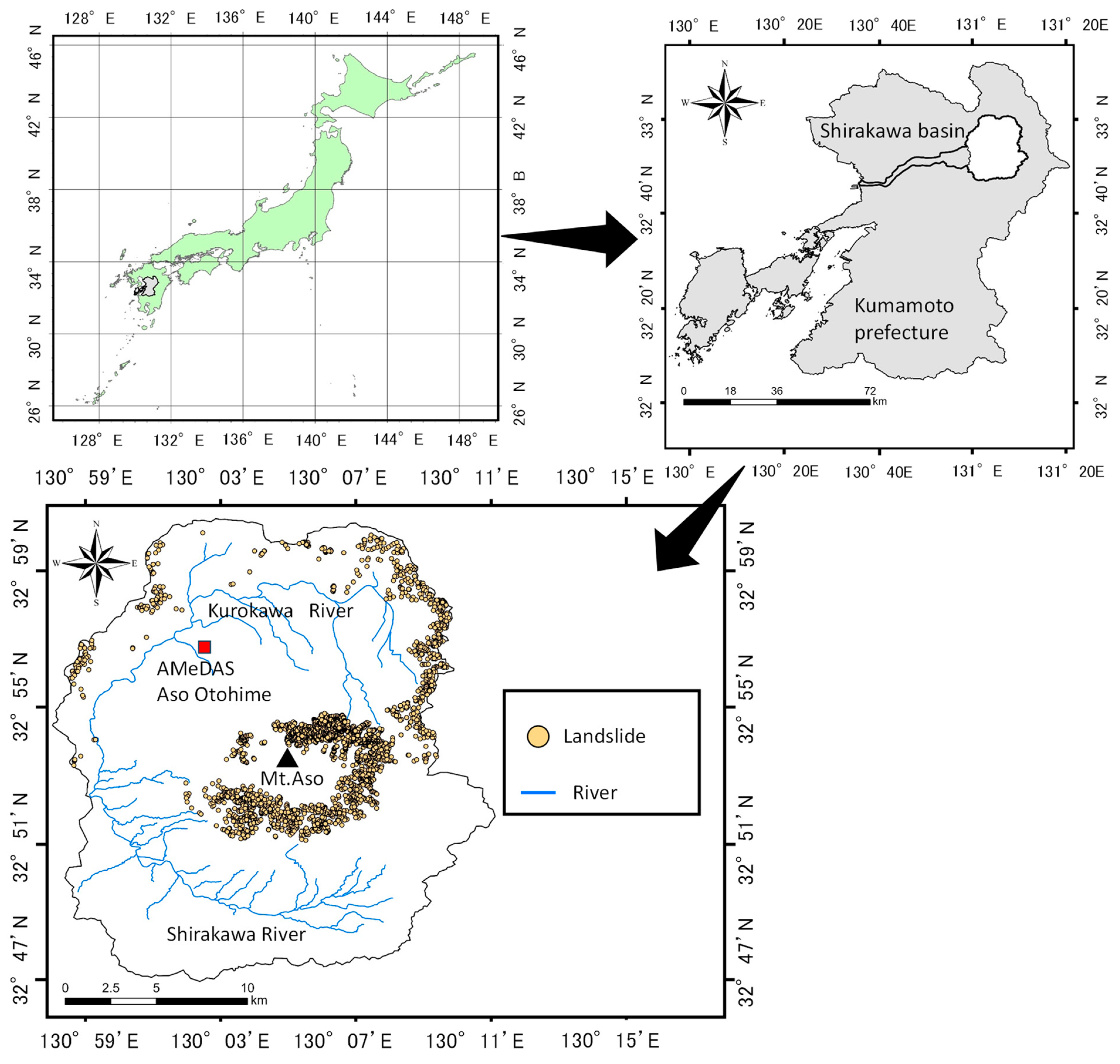
Figure 1. Location of the study area.
Water 15 03193 g001
Figure 2. Hourly rainfall and cumulative rainfall from 11 to 12 July 2012 at Aso Otohime Observatory, Kumamoto prefecture.
Water 15 03193 g002
Figure 3. The landslides caused by heavy rain. (a) Shallow landslide that occurred in Ichinomiya Town, Aso City, Kumamoto Prefecture. (b) Debris flow that occurred in Kitanosaka-nashi, Ichinomiya Town, Aso City, Kumamoto Prefecture. The photos were provided by Asia Air Survey Co., Ltd.
Water 15 03193 g003
Figure 4. Flow chart of this study.
Water 15 03193 g004
Figure 5. Distribution of the shallow landslides.
Water 15 03193 g005
Figure 6. Primary factors: (a) elevation; (b) slope angle; (c) slope aspect; (d) stream power index (SPI); (e) topographic wetness index (TWI); (f) geology; (g) vegetation.
Water 15 03193 g006aWater 15 03193 g006b
Figure 7. Triggering factors: (a) hourly rainfall; (b) effective rainfall.
Water 15 03193 g007
Figure 8. The landslide probability for each vegetation category was calculated based on the GLM. The landslide probability for each category was calculated by substituting the median value of the landslide units for the continuous variables such as elevation, slope, undulation, TWI, and hourly rainfall; the value of the reference regression coefficient (=0) for the categorical variables such as aspect, geology; and the regression coefficient for each vegetation category. Different English letters between categories indicate a significant difference at the 5% level according to the multiple comparison test (a < b). The red line indicates the cut-off value.
Water 15 03193 g008
Figure 9. Importance of factors in the RF model.
Water 15 03193 g009
Figure 10. Receiver operating characteristic curves: (a) GLM; (b) RF model.
Water 15 03193 g010
Figure 11. Response curves by GLM: (a) slope; (b) hourly rainfall.
Water 15 03193 g011
Table 1. Information about factors selected in the study.
FactorsData SourceData TypeValue Range
ElevationDEMContinuous246.51–1587.16
Slope angleDEMContinuous0.01–67.57
Slope aspectDEMCategoricaln/a
UndulationDEMContinuous0.00–342.00
SPIDEMContinuous0.00–106,087.27
TWIDEMContinuous−0.88–11.88
Geology[53]Categoricaln/a
Vegetation[64]Categoricaln/a
Hourly rainfall[65]Continuous53.4–124.46
Effective rainfall[65]Continuous57.96–249.86
Table 2. Confusion matrix.
True Condition
LandslideNon-Landslide
Prediction ConditionLandslideTPFP
Non-landslideFNTN
Table 3. Multicollinearity analysis.
FactorsVariance Inflation Factors (VIF)
Elevation2.032.01
Slope angle3.323.37
Slope aspect1.121.13
Undulation1.831.83
SPI1.001.00
TWI1.691.73
Geology1.851.83
Vegetation2.332.24
Hourly rainfall1.61n/a
Effective rainfalln/a1.49
Table 4. Results of the GLM. Variables marked in bold are those where the p-value is less than 0.05.
FactorEstimateStd. Errorz Valuep-Value
(Intercept) −9.870.62−15.96<0.05
Elevation 0.000.00−3.52<0.05
Slope angle 0.060.0111.78<0.05
Slope aspecteast1.090.432.54<0.05
northeast0.360.440.830.41
northwest0.820.431.910.06
south0.870.432.03<0.05
southeast0.840.431.950.05
southwest0.830.431.920.06
west0.800.431.860.06
Undulation 0.010.009.75<0.05
TWI −0.400.05−8.63<0.05
GeologyPre-Aso lavas−2.560.15−17.10<0.05
Unconsolidated deposits−2.420.34−7.07<0.05
Welded tuff−1.170.32−3.62<0.05
Volcanic ash (pre-caldera)−1.370.12−11.07<0.05
VegetationBamboo−13.08671.31−0.020.98
Broadleaf forests−0.090.00−0.340.74
Broadleaf secondary forest−0.940.35−2.68<0.05
Farmland−12.47141−0.090.93
Others−0.950.37−2.59<0.05
Pasture−0.870.70−1.210.23
Pine forest−0.041.02−0.040.97
Residential land−1.541.00−2.61<0.05
Riparian forest−13.281258−0.010.99
Secondary grassland1.260.1111.84<0.05
Shrub forest1.370.1310.16<0.05
Valley forest−14.341828.53−0.010.99
Wetland−12.362228.75−0.011.00
Hourly rainfall 0.050.0014.57<0.05
Table 5. AUC values of stratified 10-fold cross-validation of the GLM.
SubsetAUCSubsetAUC
10.8960.91
20.9170.90
30.9180.91
40.9290.89
50.91100.91
Table 6. Confusion matrix of the GLM.
GLMTrue ConditionSummation
LandslideNon-Landslide
Prediction ConditionLandslide3794381Precision: 0.08
Non-landslide7622,3980.003
SummationSensitivity: 0.83Specificity: 0.84Accuracy: 0.84
Table 7. AUC values of stratified 10-fold cross-validation of the RF model.
SubsetAUCSubsetAUC
10.9360.95
20.9370.96
30.9680.95
40.9590.84
50.96100.95
Table 8. Confusion matrix of the RF model.
RFTrue ConditionSummation
LandslideNon-Landslide
Prediction
Condition
Landslide4023392Precision: 0.11
Non-landslide5323,3870.002
SummationSensitivity: 0.88Specificity: 0.87Accuracy: 0.87
Disclaimer/Publisher’s Note: The statements, opinions and data contained in all publications are solely those of the individual author(s) and contributor(s) and not of MDPI and/or the editor(s). MDPI and/or the editor(s) disclaim responsibility for any injury to people or property resulting from any ideas, methods, instructions or products referred to in the content.