Article

Multi-Objective Optimal Scheduling of Generalized Water Resources Based on an Inter-Basin Water Transfer Project

1
College of Hydraulic Science and Engineering, Yangzhou University, Yangzhou 225008, China
2
Engineering Research Center of High-Efficiency and Energy-Saving Large Axial Flow Pumping Station, Jiangsu Province, Yangzhou University, Yangzhou 225009, China
3
Modern Rural Water Resources Research Institute, Yangzhou University, Yangzhou 225008, China
*
Author to whom correspondence should be addressed.
Water 2023, 15(18), 3195; https://doi.org/10.3390/w15183195
Submission received: 7 June 2023 / Revised: 3 September 2023 / Accepted: 5 September 2023 / Published: 7 September 2023
(This article belongs to the Section Water Resources Management, Policy and Governance)

Abstract

:
For inter-basin water transfer (IBWT) projects, the conflict between social, economic, and ecological objectives makes water allocation processes more complex. Specific to the problem of water resource conflict in IBWT projects, we established an optimal allocation model of generalized (conventional) water resources (G (C) model) to demonstrate the advantages of the G model. The improved multi-objective cuckoo optimization algorithm (IMOCS) was applied to search the Pareto frontiers of the two models under normal, dry, and extremely dry conditions. The optimal allocation scheme set of generalized (conventional) water resources (G (C) scheme set) consists of ten Pareto optimal solutions with the minimum water shortage selected from the Pareto optimal solutions of the G (C) model. The analytic hierarchy process (AHP) combined with criteria importance using the inter-criteria correlation (CRITIC) method was used to assign weights of evaluation indexes in the evaluation index system. The non-negative matrix method was employed to evaluate the G (C) scheme set to determine the best G (C) scheme for the Jiangsu section of the South-to-North Water Transfer (J-SNWT) Project. The results show that (1) the Pareto frontier of the G model is better than that of the C model, and (2) the best G scheme shows better index values compared to the best C scheme. The total water shortages are reduced by 254.2 million m3 and 827.9 million m3 under the dry condition, respectively, and the water losses are reduced by 145.1 million m3 and 141.1 million m3 under the extremely dry condition, respectively. These findings could not only provide J-SNWT Project managers with guidelines for water allocation under normal, dry, and extremely dry conditions but also demonstrate that the G model could achieve better water-allocation benefits than the C model for inter-basin water transfer projects.

1. Introduction

Water resources play fundamental roles in supporting sustainable socio-economic development and a healthy and stable ecological environment [1,2]. Moreover, water resources are characterized by uneven spatio-temporal distributions, which often do not match the level of socio-economic development and industrial structure layout [3]. For this purpose, people take various engineering and non-engineering measures to rationalize the allocation of water resources, i.e., water resources allocation. Inter-basin water transfer projects (IBWT) are complicated. They transfer water from water-sufficient basins to water-deficient basins to alleviate water shortages in water-deficient basins, which is an engineering measure to allocate water resources in water-deficient basins after the third supply and demand balance analysis [4,5]. At present, many countries around the world have built IBWT projects—for example, the South–North Water Transfer (SNWT) Project in China; the Snowy Mountains Water Transfer Project in Australia [6]; the California Water Transfer Project; and the Central Project in Utah, USA [7]. It is well known that China’s SNWT Project has become the world’s largest project scale and the most economically beneficial IBWT project [8].
Under the condition of limited water resources, alleviating the conflicts between different water use sectors and improving the efficiency of integrated water use are required to achieve the multi-objective allocation of water resources [9]. As the requirements of different water users increase, water-allocation problems often involve multiple water sources, multiple paths of water transmission, and multiple water-allocation scenarios, gradually forming a complicated system optimization problem [3]. For IBWT projects, the co-existence of natural and artificial connections between rivers and lakes, as well as the series-parallel relationship between them, make the water allocation processes more complex [10]. In addition, the dynamic and uncertain nature of the water resource allocation process further increases the difficulty of water resource allocation in IBWT projects [11]. Therefore, how to allocate water resources relying on IBWT projects is an important issue in the water resources domain.
The optimal allocation of water resources is one of the most effective ways to alleviate the conflict between water supply and demand [12], referring to the rational scheduling and allocation of limited water resources within a specific basin or region in time, space, and among different beneficiaries by using system analysis theory and optimization techniques [13]. As a result, the optimal allocation of water resources is increasingly being recognized as a strategic issue [14,15,16]. The optimal allocation of a water resources model can produce an optimal solution to the decision-making problems in water resources system management. Methods previously used for single-objective optimization of water resources systems include linear programming [17], nonlinear programming [18], and dynamic programming [19]. However, the water resource allocation problem relying on the IBWT project is a complex multi-objective optimization problem involving multiple water sources, multiple users, and multiple water transmission routes and links. When the decision-making problem needs to be solved for multiple objectives, traditional single-objective scheduling can no longer meet people’s needs. Recently, in order to solve the multi-objective optimization allocation problem, many multi-objective optimization algorithms, such as the NSGA- II [20], the slime mold algorithm [21], the simulated annealing particle swarm optimization algorithm [22], and the particle swarm algorithm [23], have been successfully used for solving various water resource optimization problems. However, these multi-objective algorithms suffer from slow late convergence and easily fall into locally optimal solutions. The cuckoo optimization algorithm is a new swarm intelligence optimization algorithm proposed by Yang and Deb in 2009 [24], which has been widely used in some complex engineering problems due to its advantages, such as fewer parameters and simple principles for easy implementation. Yang and Deb (2013) further designed the multi-objective cuckoo optimization algorithm, and the study showed that the multi-objective cuckoo optimization algorithm exhibited better convergence and performance compared with other algorithms [25].
In many watersheds in China, especially in arid and semi-arid areas, water shortages often occur when local demand for water resources exceeds available supply [26]. China’s largest IBWT project, the SNWT Project, transfers water resources from the Yangtze River basin to the northern region to alleviate water shortages [27]. In the past, many studies have been conducted to investigate the optimal allocation of water resources for different water transfer projects. For example, Fang et al. [28] established a multi-objective optimal allocation model of water resources with minimum total pumpage and maximum water supply rate as the objective function and obtained the water resource allocation scheme under the different incoming water conditions. Guo et al. [29] established a multi-objective optimal allocation model of the IBWT project to obtain solutions under the different incoming water conditions. Yan et al. [30] presented a new integrated model for optimal water resource allocation in a typical river basin and obtained the optimal solution set for the optimal allocation of water resources. However, most of these studies use conventional water resources (surface water) as input conditions to establish the optimal allocation model of conventional water resources, and there is a lack of understanding of the concept of generalized water allocation, resulting in a significant lack of research on using unconventional and conventional water resources as input conditions to establish the optimal allocation model of generalized water resources. In addition, during the operation of IBWT projects, evaporation, seepage loss of water, and discarded water from the transferred lakes seriously reduce the efficiency of water resource allocation [31,32].
The over-exploitation of conventional water resources has resulted in the decay of water in rivers and the lowering of groundwater levels, which ultimately damage the ecological environment and threaten people’s normal production and life [33]. With the increasing problem of water scarcity, people are not limited to the exploitation of conventional water resources (surface water) but also pay more attention to the use value of unconventional water resources (e.g., soil water) [34]. The concept of generalized water resource allocation has largely enriched the allocation of water sources, allocation objects, and allocation indexes and has important guiding significance for future water resource allocation [35]. Therefore, it is necessary to establish a water resource optimal allocation model to reduce water loss and improve the comprehensive utilization efficiency for IBWT projects on the basis of the concept of generalized water resources allocation so as to reduce the negative impact of water loss on the water resources system.
This study aims to construct a multi-objective optimal allocation model based on the concept of generalized water resources allocation, taking into account the overall amount of water discarded from lakes and reservoirs and evaporation and seepage losses on the route of water transmission, combined with unconventional water resources data (soil water) from satellite remote sensing inversion, and propose a best G scheme that can match the water demand of each water use sector so as to reduce the impact of water loss on water resource allocation.

2. Methods

2.1. Optimal Allocation Model of Generalized Water Resources

The optimal allocation model of water resources includes two parts: objective function and constraints. The optimization model uses a month as the minimum calculation time scale. The pumping station pumping capacity is used as the decision variable [28,29].
Considering the introduction of non-conventional water resources (soil water) as one of the input conditions of the model, the optimal allocation model of generalized water resources (G model) is established with surface water and soil water as the model input conditions. To verify the superiority of the G model, the optimal allocation model of conventional water resources (C model) is established with surface water as the model input condition to compare the performance of the G model.
In the objective function minimizing total water shortage, the G model has two water sources of water supply: surface water and soil water, and the C model has one water source of water supply: surface water. Among the constraints, the G model has seven constraints, including water balance constraint, soil water depth constraint, lake storage constraint, pumping capacity constraint, sluice capacity constraint, minimizing water transfer level, and non-negative constraint. The C model has six constraints, including water balance constraint, lake storage constraint, pumping capacity constraint, sluice capacity constraint, minimizing water transfer level, and non-negative constraint.

2.1.1. Objective Functions

In optimizing the allocation of water resources for the water resource system, the water demand of different water-using sectors should be fully satisfied so that the total water shortage of the system can be minimized. Likewise, evaporation, seepage losses, and water loss from storage lakes can seriously affect the efficiency of water allocation. Thus, the objective of water resource allocation is to minimize water shortage for different users and minimize water loss in the water resources system. The objective function is calculated as follows.
(1)
Minimizing total water shortage
f 1 = t = 1 T i = 1 m W i , t D - k j = 1 l j W i , t , k j S
where f1(m3) is the total amount of water shortage for each user’s agricultural, industrial, domestic, ecological environment, and shipping in the water resources system throughout the dispatch period, and T is the total number of months in the scheduling period. M is the total number of allocation units of the water resources system, WDi,t (m3) is the water demand of unit i at month t of the water resource system, lj is the total number of water sources (surface water, soil water, etc.) supplied by the water resource system to the j user, and WSi,t,kj (m3) is the water supply from the kj source of the water resource system to unit i at the month t.
(2)
Minimizing water loss in water resources systems
f 2 = t = 1 T i = 1 I W i , t L + W i , t S + j = 1 J W j , t E + W j , t S
where f2 (m3) is the total water loss of the water resources system during the dispatch period; I is the total number of river cells; WLi,t and WSi,t (m3)are the water loss by seepage and water disposal in month t for river cell i, respectively; J is the total number of lake cells; and WEj,t and WSj,t (m3) are the evaporation and disposal of water from the lake j unit in month t, respectively.
The main equation of WE in Equation (3) is as follows.
W E = 0.1 E W F
where WE (m3) is the monthly water surface evaporation volume, Ew (mm) is the monthly water surface evaporation, and F (km3) is the monthly average water surface area.
The river leakage loss WL is calculated by the Kostiakov formula [36], and the key formula is shown as follows.
W L = A Q 0 1 m / 100
where WL (m3/s/km) is the leakage loss per unit canal length, Q0 (m3/s) is the average channel traffic, and A and m are the soil permeability parameters.

2.1.2. Constraints

There are six main constraints, as follows.
(1)
Water balance constraint
V i , t + 1 = V i , t + Q i , t + D J i , t + P i + 1 , t - D C i , t - W i , t D 1 - W i , t E - W i , t S
where i is the lake number (lake i); Vi,t+1 and Vi,t (m3) are the water storage of lake i at time t and time t + 1, respectively; Qi,t (m3/s) is the natural runoff of lake i at time t; DJi,t and DCi,t (m3) are the inflow and outflow of lake i at time t, respectively; and Pi+1,t (m3) is the amount of water released into lake i + 1 and at time t.
(2)
Soil water depth constraint
0 H H max
where H is the soil water depth; Hmax is the maximum depth of soil water.
(3)
Lake storage constraint
V i , t , m i n V i , t V i , t , m a x
where Vi,t,min and Vi,t,max (m3) are the minimizing and maximizing the water storage capacity of lake i at time t, respectively.
(4)
Pumping capacity constraint
0 D J i , t D J i , t , m a x   0 D C i , t D C i , t , m a x
where DJi,t,max and DCi,t,max (m3) are the maximizing pumping capacity of the pumping station of lake i at time t, respectively.
(5)
Sluice capacity constraint
W i , t , m i n S W i , t S W i , t , m a x S
where WSi,t,min and WSi,t,max (m3) are the minimizing and maximizing overflow capacity of gate i at time t, respectively.
(6)
Minimizing water transfer level
In general, the pumping of lake water is stopped when the lake level is lower than the limit level.
(7)
Non-negative constraint
All variables in the optimal water allocation model cannot be negative.

2.2. Improved Multi-Objective Optimization Algorithm

The multi-objective cuckoo optimization algorithm suffers from the same problems as other multi-objective algorithms of slow late convergence and easily falls into local optimal solutions. Therefore, the improved multi-objective cuckoo optimization algorithm (IMOCS) [37] is used to solve the G model and the C model in the study. The IMOCS is given as follows: (1) to improve the population evolution strength and avoid the algorithm from falling into local convergence, the cosine strategy is used to realize the dynamic change of Pa, and (2) by introducing the population variation mechanism, the quality of the initial solution in the evolutionary algorithm will affect the convergence speed as well as the final optimization goal during the algorithm’s evolution. The optimal individuals of the multi-objective cuckoo optimization algorithm are mutated for each generation to further improve the quality of the population.

2.2.1. Dynamic Discovery Probability

In the multi-objective cuckoo optimization algorithm, the nest position is updated when using Lévy flight, and a number a (0 ≤ a ≤ 1) is generated randomly. If aPa, the nest is updated randomly once, and then the best nest location is retained. A larger Pa is used at the early stage of the algorithm operation to find the optimal solution quickly, and a smaller Pa is used at the later stage of the operation to obtain the optimal convergence result, which is used to improve the accuracy of the algorithm for finding the optimal solution. Thus, the cosine strategy is used to achieve the dynamic change of Pa so that Pa decreases gradually as the algorithm proceeds [37].
The Lévy flight characteristic [24] is shown as follows.
x i ( t + 1 ) = x i ( t ) + α L β
where xi(t + 1) is the new egg produced by the ith cuckoo at generation t + 1; α is the step control amount, α = α0(xj(t) − xi(t)), where α0 is a constant; ⊕ is point-to-point multiplication; and L(β) is the search step length and obeys the Lévy distribution, i.e., L(β)~u = t−1−β, 0 < β ≤ 2.
Decreasing cosine strategy.
P a = P a , m a x c o s π 2 × T 1 T m a x 1 + P a , m i n
where Pa,max, and Pa,min are the control parameters of Pa, both located in the range of 0~1; T is the current evolutionary generation; and Tmax is the maximum evolutionary generation.

2.2.2. Mechanisms of Population Variation

The multi-objective cuckoo optimization algorithm initial solution generation method has great randomness, and the population size must be increased to obtain a high-quality initial population, but the increase in the population size will inevitably affect the operation of the computer and lead to a decrease in the speed of the merit search. For this reason, this study introduces a variation mechanism for the first stratum of Pareto in each generation to further improve the quality of the population [37]. The mutation mechanism is as follows.
x t , b 2 = x t , b 1 + [ a 1 c o s π 2 × T 1 T m a x 1 ] ε
where xt,b2 and xt,b1 are the nest locations before and after the mutation; a1 is the control parameter; ε is a 1 × d vector, obeying the standard normal distribution; and d is the dimension of the optimization problem.

2.3. Evaluation of Non-Inferior Solutions for Scheduling of Water Resources

The Pareto solution set for optimal scheduling of water resources can be obtained by solving the G and C models, while the best equilibrium solution from the set of alternatives should be selected for the actual scheduling decision so as to achieve the maximization of the comprehensive benefits. Therefore, it is necessary to understand the preferences for decision-making while also making another decision on the set of options based on the indexes on the basis of socio-economic costs, and the optimal water resource allocation scheme is selected. In addition, the selection of the optimal water resources allocation scheme is a complex decision-making process involving multiple sectors and aspects. If only the total water shortage and the water loss are used to consider the two aspects, prone to decision-making bias, it affects the optimal allocation of the water resources scheme. The following work needs to be carried out: one, enrich the content of decision-making indicators and construct an index system to evaluate the optimal allocation of water resources; and two, adopt appropriate empowerment methods and decision-making methods.

2.3.1. Index System for Evaluating Water Resources Optimization Allocation

Research on the optimal allocation of water resources aims to achieve mutual assistance and mutual adjustment between multiple water sources in multiple water transmission processes to multiple users. The water resources within the water resources system can be fully and reasonably utilized. Therefore, the scheduling of the water resources system should make full use of natural incoming water as far as possible, avoid lake abandonment, increase the total water supply of the whole water resources system, and alleviate the degree of water shortage in different water-receiving areas. From this point of view, the evaluation indexes such as drainage volume, abandoned water, water loss, and total pumped water should be selected. When carrying out water supply in the water resources system, the effectiveness of pumping stations cannot be ignored, and the benefits of a small amount of water supply by increasing the amount of water pumped should be avoided, striving to achieve a balance between operating cost (amount of water shortage) and water supply (total amount of water pumped) in the water resources system. Finally, the optimal allocation model of the water resources index system is constructed and shown in Table 1.

2.3.2. Index Weight Quantification and Evaluation Methods

Analytic hierarchy process (AHP) is a systematic analysis method based on stratification, comparative judgment, and synthesis [38]. It mainly considers the subjective understanding of evaluation indexes by the evaluation subject and focuses more on qualitative judgment and analysis than the general quantitative method, which is one of the more widely used methods in the subjective empowerment method at present.
Criteria importance through inter-criteria correlation (CRITIC) is an objective assignment method, which is determined based on the analysis of the correlation between the data of each index of the index system [39]. CRITIC not only analyzes the influence of index variation on weights in the determination of index weights but also takes into account the existence of conflicting relationships between indexes, which is better than other objective weighting methods, such as the entropy weighting method, in terms of application effect.
By combining subjective and objective weights in a certain ratio, the combined weigh method (AHP-CRITIC method) takes into account the subjective intention of decision-makers and reflects the objective laws of the data itself, making the weighting results more scientific and reasonable [40]. Following this idea, AHP is used to determine the subjective weights, CRITIC is used to determine the objective weights, and Equation (13) is used to calculate the combined weights as a basis for differentiating the importance of each index.
w i = μ w i 1 + ( 1 μ ) w i 2
where μ is the preference coefficient between subjective weights and objective weights, 0 ≤ μ ≤ 1.
Non-negative matrix factorization [41] performs a non-negative decomposition of the evaluation matrix into a product of a row vector and a column vector with the largest approximation, where the column vector is the metric vector in the matrix of the program indexes and the elements of the row vector are the degrees of merit of the evaluation objects of the corresponding program. The method can solve the problem that evaluation indexes are not metric, extract the main features of the evaluation matrix via dimensionality reduction, and weaken the negative influence of index weights on the evaluation results. The main formula of NMF is as follows.
v i = j = 1 n z i j × h j / j = 1 n h j 2 ,   ( i = 1 , 2 , , m ) h j = i = 1 m z i j × v i / i = 1 m v i 2 ,   ( j = 1 , 2 , , n )
where n is the number of solutions in the Pareto optimal solutions; m is the number of evaluation metrics; V = (v1, v2, …, vm)T is the basis vector, vi∈[0, 1], ∑vi2 = 1; H = (h1, h2, …, hn) is the weight vector, hj∈[0, +∞), and a larger hj indicates a better water allocation effect of solution j; and zij is the normalized value of solution j corresponding to index i.

2.3.3. Determination of the Optimal Allocation Schemes of Water Resources

The optimal allocation schemes of generalized water resources (G schemes) and the optimal allocation schemes of conventional water resources (C schemes) are selected from the Pareto optimal solutions of the G model and the C model, respectively. These schemes form a G (C) scheme set. Moreover, there are m G (C) (m ≥ 1) scheme sets under m incoming water conditions. Specifically, the Pareto optimal solution of the G (C) model contains N (N is the algorithmic population size) G (C) schemes with a wide range of distribution of the objective values of the schemes, which will increase the difficulty and uncertainty of decision-making if all the schemes are to be evaluated. For convenience, ten Pareto optimal solutions, which correspond to the minimum water shortage volumes of the G (C) model, are selected from the G (C) scheme set.
Considering the requirements of water users, we are mainly concerned about three incoming water conditions, i.e., normal condition (50% incoming water frequency), dry condition (75% incoming water frequency), and extremely dry condition (95% incoming water frequency). Then, the best G (C) scheme can be determined by evaluating the G and C scheme sets under a certain incoming water condition.

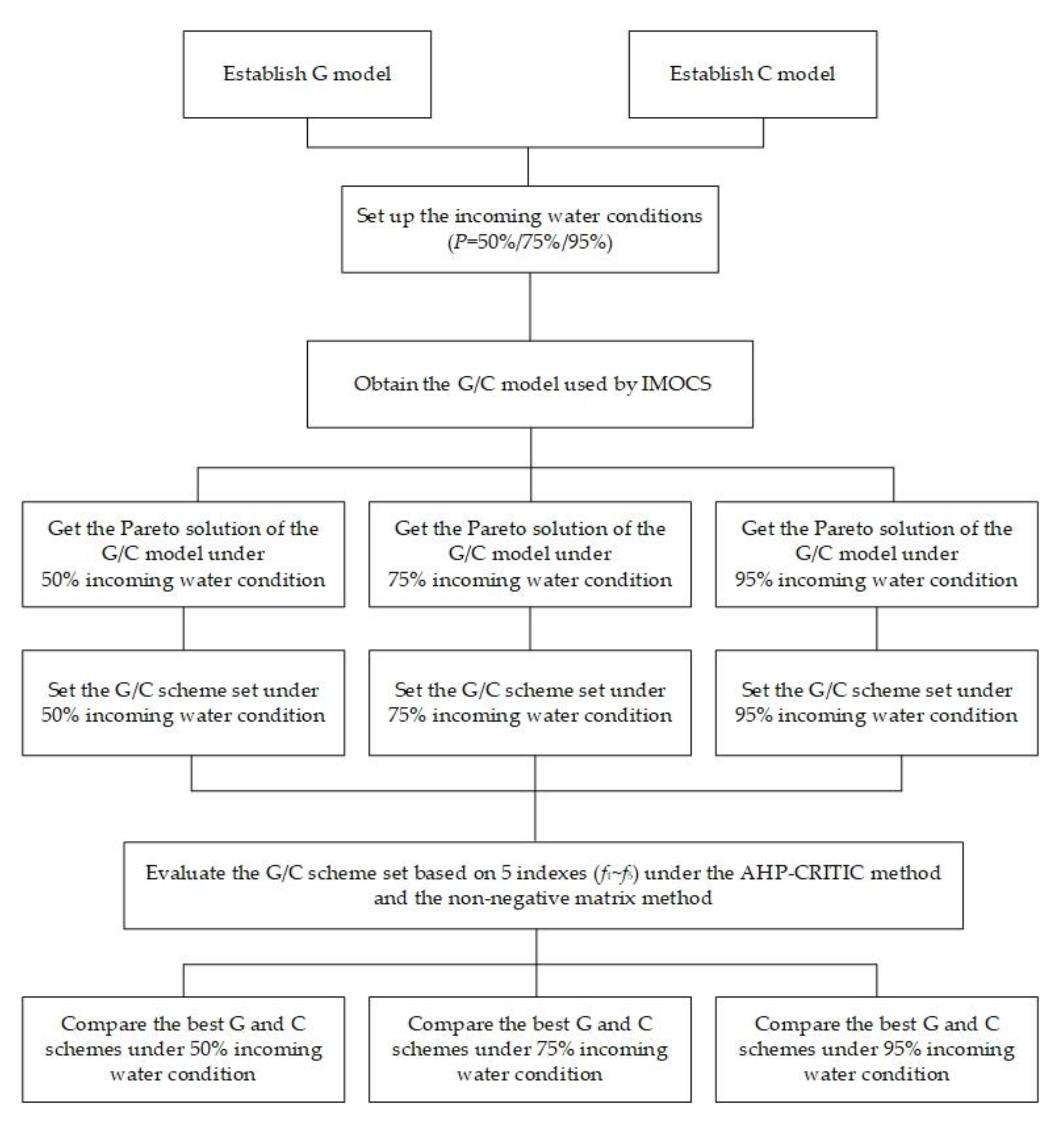
2.3.4. Evaluation of the Optimal Allocation Schemes and Technology Road Map of the Study

The G and C scheme sets can be obtained by solving the G and C models. We can construct the index system for evaluating the G (C) scheme set according to the index system for evaluating the optimal allocation model of water resources. Determination of index weights for the G (C) scheme set is based on the AHP-CRITIC method, in which subjective weighting is given by the AHP method, and objective weighting is given by the CRITIC method. The non-negative matrix method is used to evaluate the G (C) scheme set for the different incoming water conditions and obtain the best G (C) scheme for the different incoming water frequencies. We can compare the best G and C schemes under the different incoming water conditions to validate the superiority of the G model.
To better illustrate the idea of this study, the technology road map is shown in Figure 1.

3. Study Area and Data
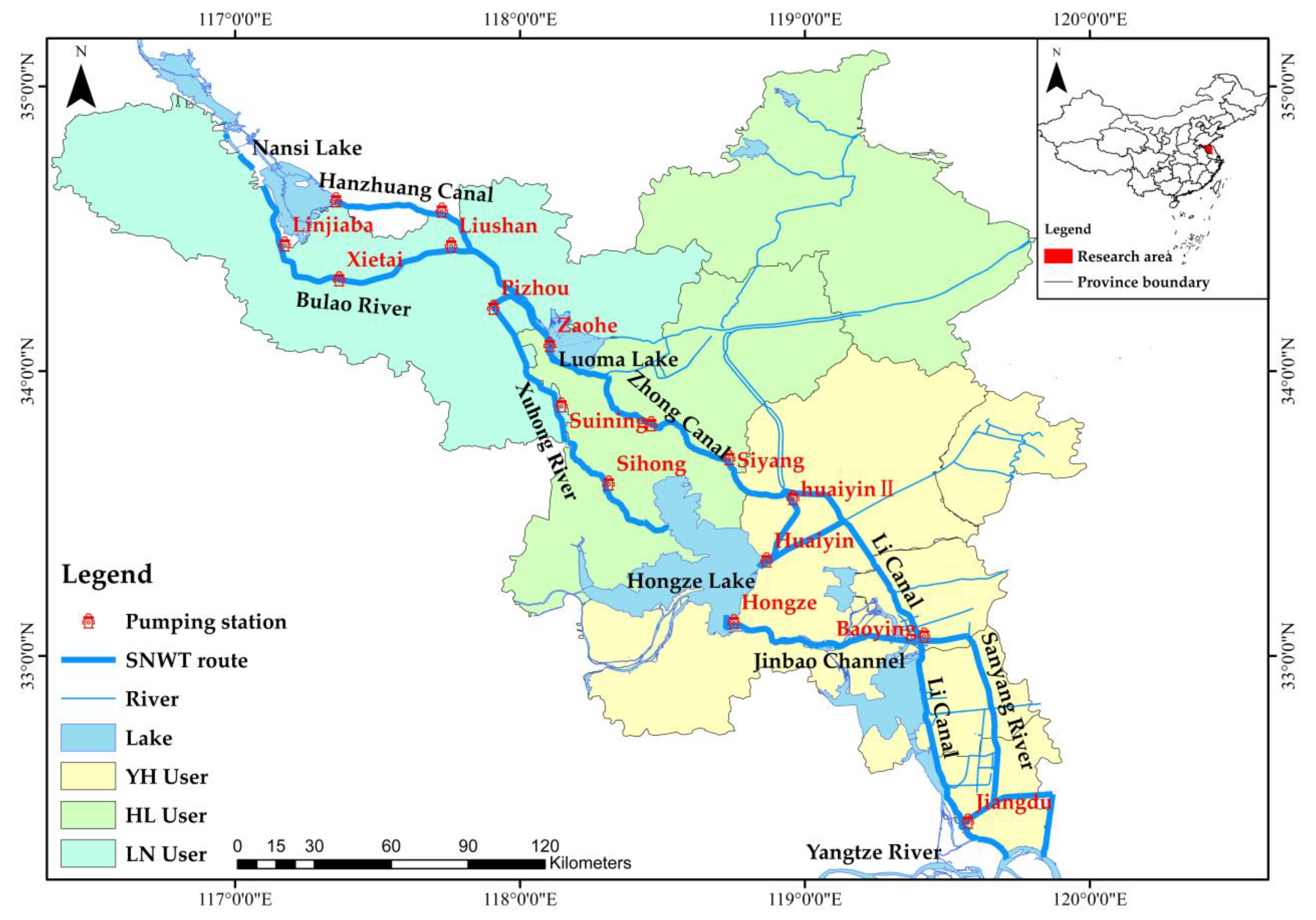
3.1. Study Area

The J-SNWT Project is one of the major IBWT projects in China and is a significant strategic infrastructure used to alleviate the severe water shortage in the north of China. It expands the scale of water transfer and extends northward based on the existing river water transfer project in Jiangsu Province. We focus on J-SNWT, as shown in Figure 2. As the starting section of the SNWT Project, the J-SNWT Project aims to solve the water tension problem of six cities in Jiangsu. Along the project route, there are storage lakes such as Hongze Lake, Luoma Lake, and Nansi Lake. The water storage characteristics of the three lakes are found in the feasibility evaluation report of the J-SNWT Project, as detailed in Table 2. The route from Yangtze River to Nansi Lake can be divided into three sections, with two pumping stations set in each section, for a total of six water lifting steps. The features of the pumping stations and sluices in the J-SNWT Project are also provided by the feasibility evaluation report of the J-SNWT Project and are detailed in Table 3. These storage lakes and pumping stations at all levels make the water resources system of the J-SNWT Project have a large storage capacity. The system is generalized according to the main composition of the J-SNWT Project and the connection relationship of the mainline tributaries. To fully reflect the storage capacity of the lake and the actual engineering operation characteristics of the J-SNWT Project, the Jiangsu section is mainly divided into seven water-receiving areas, the agricultural water-receiving area of Anhui Province is assigned to Hongze Lake, and Shandong Province is generalized as a water user as a whole. The schematic diagram of the generalized system is shown in Figure 3.

3.2. Data

3.2.1. Surface Water

By analyzing the historical hydrological series incoming water information from the Huaihe Hydrological Yearbook, the Pearson Ⅲ type (P-Ⅲ) curve is used for hydrological frequency calculation to derive the annual runoff at each design frequency, and then the year in which the annual runoff is close to the design value is selected as the representative year. We take the runoff process of the planning level year at the design frequency of p = 50%, 75%, and 95% for analysis and calculation, which is carried out using the periodical portal. The calculated hydrological frequency of runoff from each lake is shown in Table 4.

3.2.2. Soil Water

Historical soil moisture data of J-SNWT provided by the Global Land Data Analysis System (GLDAS_NOAH025_M_2.1) (https://disc.gsfc.nasa.gov/datasets (accessed on 28 October 2022)) [42] are categorized by Arc GIS into six water-receiving areas. The Pearson III type (P-III) curve is used for hydrological frequency calculation to derive the soil moisture at each design frequency, and then the year in which the soil moisture is close to the design value is selected as the representative year. We take the soil water change process of the planning level year at the design frequency of p = 50%, 75%, and 95% for analysis and calculation. The depth of soil water content is determined based on the rooting depth of different crops grown by agricultural water users in the six water-receiving areas. Determination of dryland soil moisture content and paddy field soil moisture content based on the attributes of the crops to be grown is performed, and then soil water content is calculated for each of the six water-receiving areas under normal, dry, and extremely dry conditions. Representative years of soil water in each water-receiving area are shown in Table 4.
The water demands in the seven water-receiving areas mainly include agricultural, industrial, domestic, ecological environment, and shipping. According to the Chinese standard [43] the Water Quota Method is used to calculate the water demand for the domestic, agricultural, and industrial sectors by integrating the water quota and activity level of each section with reuse and loss rates. The water requirements for ecology and shipping are provided by the feasibility evaluation report of the J-SNWT Project. The current and planned water allocation years are 2018 and 2030, respectively. Figure 4 shows the water demand of each water user in 2030 under normal, dry, and extremely dry conditions, respectively.

4. Results

4.1. Multi-Objective Optimal Allocation of Water Resources Based on the J-SNWT Project

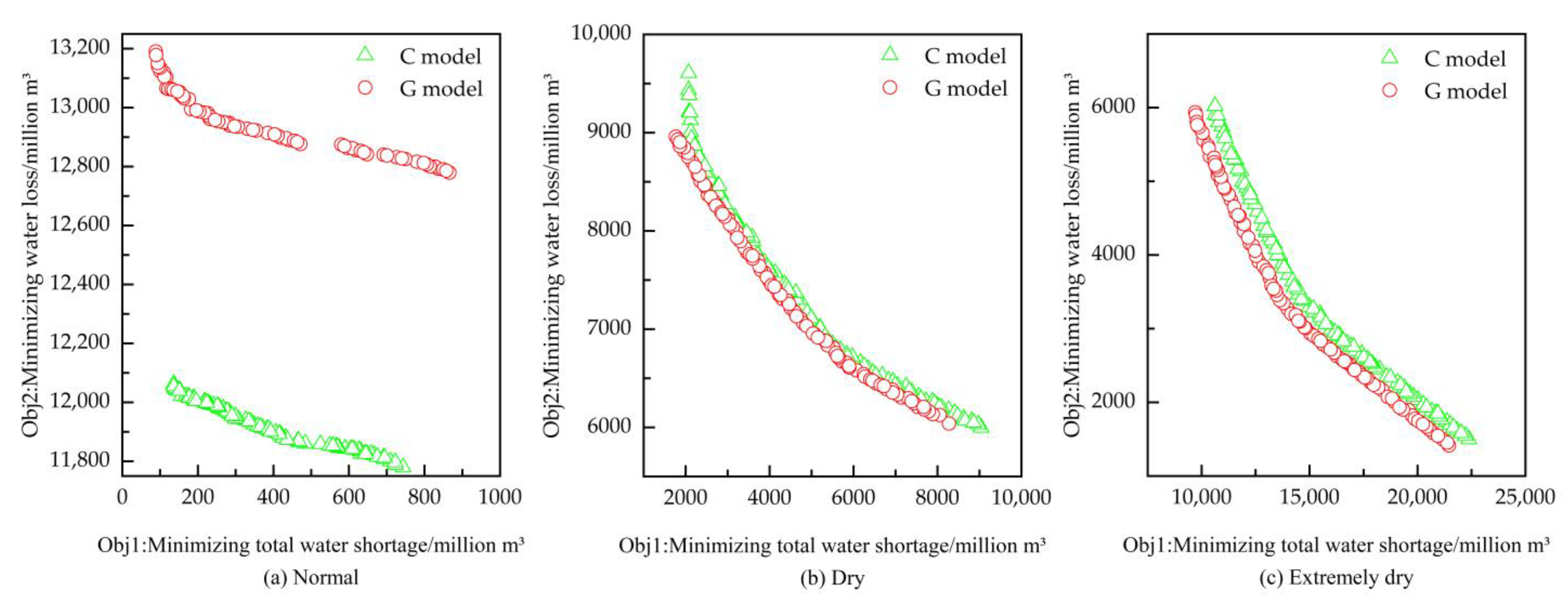
4.1.1. Pareto Frontiers of the G and C Models

IMOCS is used to solve the G and C models; the population size of IMOCS is 100, and the maximum number of iterations is 2000.
Figure 5 shows the Pareto frontiers obtained after 2000 iterations of the G and C models under normal, dry, and extremely dry conditions. The target values of total water shortage in the receiving area of the G model, as shown in Figure 5a–c, range [88.5, 865.9] million m3, [1765.3, 8275.4] million m3, and [9704.5, 21,450.3] million m3, and the target values of system water loss range [12,779.3, 13,190.7] million m3, [6040.0, 8959.7] million m3, and [1414.7, 5938.5] million m3 under the normal, dry and extremely dry conditions, respectively. As shown in Figure 5a–c, the distribution of the total water shortage in the water-receiving area of the C model ranges [135.9, 743.0] million m3, [2068.8, 9038.9] million m3, and [10,615.3, 22,380.1] million m3. The distribution of system water loss target values ranged [11,779.8, 12,063.0] million m3, [5999.2, 9608.5] million m3, and [1501.0, 6024.8] million m3.

4.1.2. Pareto Optimal Solutions Box Diagram of G and C Models

The box plots of water shortage and system water loss for the G and C models are shown in Figure 6. Figure 6a shows that the total water shortage of the G model under the normal, dry, and extremely dry conditions is reduced by 47.4~929.8 million m3 compared to the C model. This indicates that the G model is more efficient for water resource utilization than the C model. As shown in Figure 6b, the G model reduces the water loss by 86.3 million m3 compared to the C model under extremely dry conditions. The C model produces more general Pareto optimal solutions than the G model under dry conditions, but these solutions are dominated by the Pareto optimal solutions of the G model.

4.2. Optimal Allocation Scheme Set of Water Resources Based on the J-SNWT Project

4.2.1. Filtering Pareto Optimal Solutions of G (C) Model

Under an incoming water condition, the Pareto frontier of the G (C) model contains many schemes, and the target values of each scheme are widely distributed. If all schemes are considered in the G (C) scheme set, it will increase the decision-making difficulty of the water resource allocation schemes. Therefore, the 10 Pareto optimal solutions with the minimum target of water shortage in the water-receiving area are selected in the G (C) scheme set.

4.2.2. Quantification of the Index Weights for the G (C) Scheme Set

The AHP method is first applied to calculate the subjective weights to the G (C) scheme set, and then the CRITIC method is used to determine the objective weights. On the one hand, the managers of government would prefer lower values of total water shortage and total pumped water. On the other hand, the managers of J-SNWT would prefer a lower value for abandoned water and water loss. In the subjective allocation, the water loss is considered the primary index, the water shortage is assigned the second index, and the drainage volume and the abandoned water are considered to have the lowest weight because they are unavoidably present under normal conditions. The water loss is the most important index, so it is assigned the greatest weight. The total water shortage and the abandoned water are equally important, and they are assigned the same weight. The drainage volume and the total pumped water are given smaller weights because pumping is needed to keep water available to water users under dry conditions. The weight of water loss is lower than under normal and dry conditions, and the weight of the water shortage is increased. The abandoned water, the drainage volume, and the total pumped water are gradually taken into account as they are the minor indexes under extremely dry conditions. The index weights of the G (C) scheme set for μ = 0.5 under normal, dry, and extremely dry conditions are given in Table 5.

4.3. The Best Scheme of Water Resources Based on the J-SNWT Project

4.3.1. Evaluation of the Best G Scheme

The non-negative matrix factorization method is used to evaluate the G scheme set and obtain the best G scheme under normal, dry, and extremely dry conditions, as shown in Figure 7. The best G scheme for total water shortage is 94.9 million m3, drainage volume is 1281.0 million m3, abandoned water is 7915.9 million m3, water loss is 13,139.0 million m3, and total pumping is 23,170.1 million m3 under normal conditions. The total water shortage is 1865.2 million m3, drainage volume is 8843.1 million m3, abandoned water is 3359.5 million m3, water loss is 8863.8 million m3, and total pumping is 29,869.1 million m3 under dry conditions. The total water shortage is 9792.4 million m3, drainage volume is 13,646.2 million m3, abandoned water is 0 million m3, water loss is 5766.0 million m3, and total pumping is 37,352.1 million m3 under extremely dry conditions.

4.3.2. Evaluation of the Best C Scheme

Figure 8 shows the evaluation of the non-negative matrix factorization method for the C scheme set to obtain the best C scheme under normal, dry, and extremely dry conditions. As shown in Figure 8, the best C scheme in normal conditions for total water shortage is 155.8 million m3, drainage volume is 1389.3 million m3, abandoned water is 6874.2 million m3, water loss is 12,021.7 million m3, and total pumping is 23,196.1 million m3. In the dry conditions, the total water shortage is 2119.4 million m3, drainage volume is 9616.6 million m3, abandoned water is 3303.9 million m3, water loss is 9008.9 million m3, and total pumping is 31,329.2 million m3. In extremely dry conditions, the total water shortage is 10,620.3 million m3, drainage volume is 14,088.3 million m3, abandoned water is 0 million m3, water loss is 5907.1 million m3, and total pumping is 38,411.4 million m3.

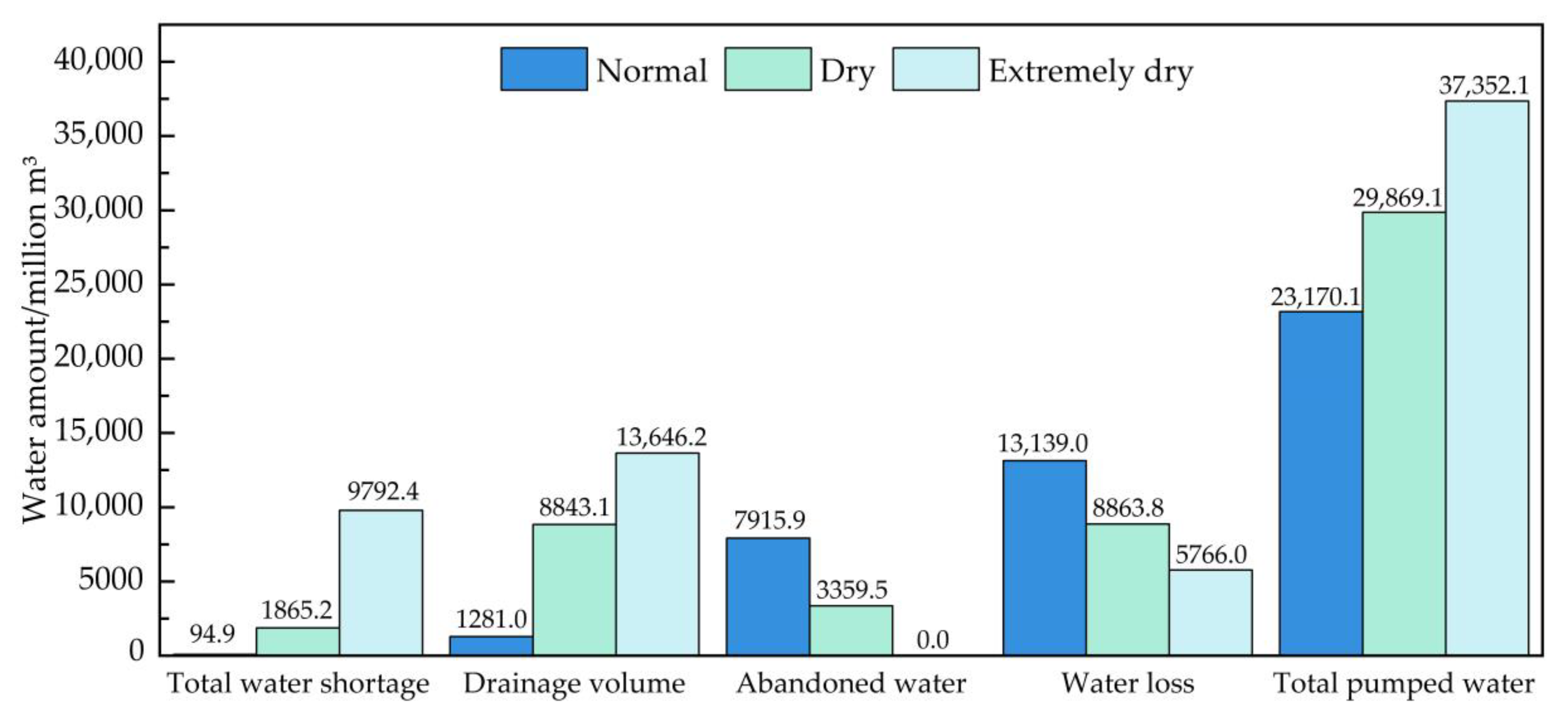
4.3.3. Comparison of the Best G Scheme and the Best C Scheme

Figure 9 provides the best G schemes and the best C schemes under normal, dry, and extremely dry conditions. Compared to the best C scheme, the best G scheme further reduces the water shortage and improves the water supply assurance level for users in the water-receiving area under the same incoming water conditions. Under normal, dry, and extremely dry conditions, the shortage of water in the water-receiving area of the best G scheme is reduced by 60.9 million m3, 254.2 million m3, and 827.9 million m3, respectively, compared with the best C scheme. In terms of operating costs, the drainage volume of the best G scheme under normal, dry, and extremely dry conditions is 108.3 million m3, 773.5 million m3, and 442.1 million m3 less than the best C scheme, and the total pumped water volume is 26.0 million m3, 1460.1 million m3, and 1059.3 million m3 lower than the best C scheme, respectively. In terms of water loss, the abandoned water and water loss of the best G scheme are 1041.7 million m3 and 1117.3 million m3 greater than the best C scheme under normal conditions. The abandoned water of the best G scheme is 55.6 million m3 more than the best C scheme, and the water loss is 145.1 million m3 lower than the best C scheme under dry conditions. The water loss of the best G scheme is 141.1 million m3 less than the best C scheme under extremely dry conditions.

5. Discussion

5.1. Effectiveness and Excellence of the G Model

The optimal allocation of water resources is not only the allocation between different water sources but also considers complicated water conveyance paths in a basin/region or across different basins/regions [44]. Based on the supply and demand relationship between water sources and water users, the optimal allocation of water resources enables the harmonious development of the regional economy and environmental protection [22]. The goal for the optimal allocation of generalized water resources is to maintain the sustainable development of the regional society–economy–ecology. The water sources of generalized water resources from the narrow sense of runoff water resources extended to precipitation and soil water. The allocation object of generalized water resources not only takes into account the economic and social water demands but also the regional ecological environment water requirements. The allocation of generalized water resources is extended from the traditional surface water supply and demand balance state to the generalized water resources supply and demand balance state. The concept of generalized water resources has greatly enriched the connotation of the allocation of water sources, allocation objects, and allocation indexes [33].
The G model aims to achieve two objectives: one is to verify whether a unified allocation of conventional and non-conventional water resources would be more helpful in alleviating water shortages in the study area. The other one is to verify whether the deployment of non-conventional water resources will reduce water loss. Therefore, we establish the G and the C models with the objective functions of minimizing water shortage and minimizing water loss in the water resource system to demonstrate the advantages of the G model.
In the case study, the Pareto frontier of the G model has a significantly higher target value for Objective 2 than the Pareto frontier of the C model under normal conditions. This result implies that in the case of sufficient incoming water, more water abandonment and water loss along the way are generated due to the limitations of the lake. In the same water shortage condition, the G model produces more water loss. However, in Objective 1, the convergence for the Pareto front of the G model is better, which shows that the G model can obtain water allocation schemes with less water shortage. The two objective values of the Pareto front for the G model are significantly lower than the two objective values of the Pareto front for the C model under dry conditions. This result implies that the Pareto frontier of the C model is trapped in the locally optimal solution and does not reach the desirable Pareto frontier. The Pareto frontier of the G model is better than that of the C model. The G scheme of the G model is better than the C scheme of the C model and can realize lower water loss under the same water shortage conditions. This is crucial for the managers of the J-SNWT Project to develop a decision-making program. The two objective values of the Pareto front of the G model are also significantly lower than the two objective values of the Pareto front of the C model under extremely dry conditions. This further indicates that the Pareto front of the G model is better than the Pareto front of the C model. The G model can obtain lower values of water shortage and water loss under the same conditions and can successfully alleviate the water shortage and water loss problems of the C model.

5.2. Optimized Allocation Scheme of J-SNWT

The current J-SNWT multi-objective water transfer model is operated based on economic factors and water demands. For example, Yu et al. [45] and Wen et al. [46] constructed a multi-objective optimal allocation model with the optimization objectives of minimizing total water shortage and minimizing water pumping. Fang et al. [28] constructed a multi-objective optimal allocation model with the optimization objectives of minimizing the total pumping and maximizing the water supply rate. The modeling ideas and methods of previous scholars and the C model are the same. Here, we combine the concept of generalized water resources with the multi-objective optimal allocation model to obtain the G model.
Multi-objective optimization analysis allows decision-makers to seek compromise allocation schemes from the Pareto frontier based on the relationships between different objectives. However, it often takes several steps to find the optimal allocation scheme from the set of Pareto solutions. The AHP-CRITIC method in this study uses quantitative objective indexes to assign Pareto solution sets. In order to avoid the subjective judgment of decision-makers, subjective and objective weights are integrated. The AHP-CRITIC method is able to consider both subjective and objective weights and can provide different decision-makers with optimal allocation schemes with different preferences. For example, J-SNWT’s managers would like to have low values for the amount of water abandoned and water loss. Under normal conditions, the increase in the amount of naturally coming water inevitably generates water loss, so water loss is mainly considered in the subjective weight allocation. Government managers prefer lower values for total water shortage. The weighting of water shortages is increased in the subjective assignment under the dry and extremely dry conditions. In a comparison of the G model and the C model scenarios on five indexes, the methodology can provide better water resource allocation schemes for J-SNWT.
The three conditions used in this study provide a useful guide for future IBWT. This study compares and analyzes the optimal schemes of the G model and the C model and selects schemes for the J-SNWT Project under normal, dry, and extremely dry conditions, which is used to verify the validity and generality of the G model. From the normal condition to the extremely dry condition, the total water shortage, the drainage volume, and the total pumped water of the best G and C schemes are gradually increasing, and their allocation results are mutually verified with those of Yu et al. [45]. The amount of water abandoned shows a decreasing trend with incoming water conditions, which is consistent with the findings of Wen et al. [46]. Under normal conditions, the amount of water abandoned and water loss of the best G scheme are higher than the best C scheme. However, the water shortage, the drainage volume, and the total pumped water of the best G scheme are lower than the best C scheme. After considering the water shortage factor, we decided to choose the best G scheme with a lower water shortage as our recommended scheme. When basins are experiencing dry and extremely dry conditions, the J-SNWT Project harmonizing non-conventional and conventional water resources can be effective in alleviating water shortages. Particularly under extremely dry conditions, it shows how the J-SNWT Project helps to secure water supply with a low inflow and high demand.
A representative year method is used to develop appropriate water allocation schemes based on normal, dry, and extremely dry conditions, as opposed to extracting effective rules from a long series of allocation processes. While this simplifies the computational and analytical workload, it also reduces the applicability of the water allocation rules. In future studies, we will collect longer historical runoff data to analyze the water allocation rules for the J-SNWT Project.

6. Conclusions

In order to quantitatively evaluate the influence of generalized water resources on the optimal allocation of water resources in IBWT projects, a G model is established and compares its configuration results with the C model to demonstrate the advantages of the former over the latter in water resource allocation. First, we establish a G model and a C model. IMOCS is used to solve the G (C) model to obtain the Pareto frontier. Second, the ten Pareto optimal solutions with the minimum water shortage are selected as the G (C) scheme set, and the water resources system evaluation index system is established. The AHP-CRITIC method assigns weights to their scheme indexes and uses the non-negative matrix factorization method to evaluate the scheme to obtain the best G (C) scheme of J-SNWT. Finally, the index values of the best G and C schemes are compared under normal, dry, and extremely dry conditions. The main conclusions are as follows:
(1) The G model demonstrates better performance than the C model. The Pareto front of the G model for Objective 1 is better than the Pareto frontier of the C model under normal conditions. The Pareto frontier of the G model is significantly better than the Pareto frontier of the C model under dry and extremely dry conditions.
(2) The best G scheme shows better index values compared to the best C scheme. In particular, under dry and extremely dry conditions, the total water shortages are reduced by 254.2 million m3 and 827.9 million m3, respectively, and the water losses are reduced by 145.1 million m3 and 141.1 million m3, respectively. The G model shows significant improvements in terms of water shortage and the cost of water supply.
This study has proved the validity and generality of the proposed G model, which can provide J-SNWT Project managers with guidelines for water allocation under normal, dry, and extremely dry conditions so that they can have some reference in their decision-making. Moreover, the inclusion of non-conventional water resources in IBWT projects can effectively alleviate the problem of water shortage.

Author Contributions

Conceptualization, H.X. and Y.X.; methodology, H.X.; software, Q.Z.; validation, H.X., Y.X. and S.L.; formal analysis, H.X. and Q.M.; investigation, Y.X.; resources, T.S.; data curation, H.X., Q.M. and T.S.; writing—original draft preparation, H.X.; writing—review and editing, Y.X. and S.L.; visualization, Q.M.; supervision, S.L.; project administration, Y.X.; funding acquisition, Y.X. and S.L. All authors have read and agreed to the published version of the manuscript.

Funding

This research was supported by the Open Project Program of Engineering Research Center of High-efficiency and Energy-saving Large Axial Flow Pumping Station, Jiangsu Province, Yangzhou University (Grant No. ECHEAP013); the Natural Science Foundation of Jiangsu Province (Grant No. BK20200958; and Grant No. BK20200959); the National Natural Science Foundation of China (Grant No. 52009116); and the China Postdoctoral Science Foundation (Grant No. 2018M642338).

Data Availability Statement

The data presented in this study are available on request from the corresponding author. The processed data are not publicly available as the data also form part of an ongoing study.

Conflicts of Interest

The authors declare no conflict of interest.

Abbreviations

IBWTInter-basin water transfer projects.
SNWTThe South–North Water Transfer project.
J-SNWTThe Jiangsu section of the South-to-North Water Transfer.
G modelOptimal allocation model of generalized water resources.
C modelOptimal allocation model of conventional water resources.
IMOCSImproved multi-objective cuckoo optimization algorithm.
AHPAnalytic hierarchy process.
CRITICCriteria importance through inter-criteria correlation.
G schemeThe optimal allocation scheme of generalized water resources.
C schemeThe optimal allocation scheme of conventional water resources.

References

  1. Cosgrove, W.J.; Loucks, D.P. Water management: Current and future challenges and research directions. Water Resour. Res. 2015, 51, 4823–4839. [Google Scholar] [CrossRef]
  2. Dong, C.; Schoups, G.; Giesen, N.V.D. Scenario development for water resource planning and management: A review. Technol. Forecast. Soc. Chang. 2013, 80, 749–761. [Google Scholar] [CrossRef]
  3. Li, Y.; Cui, Q.; Li, C.; Wang, X.; Cai, Y.; Cui, G.; Yang, Z. An improved multi-objective optimization model for supporting reservoir operation of China’s South-to-North Water Diversion Project. Sci. Total Environ. 2017, 575, 970–981. [Google Scholar] [CrossRef]
  4. Akron, A.; Ghermandi, A.; Dayan, T.; Hershkovitz, Y. Interbasin water transfer for the rehabilitation of a transboundary Mediterranean stream: An economic analysis. J. Environ. Manag. 2017, 202, 276–286. [Google Scholar] [CrossRef]
  5. Dou, X. China’s inter-basin water management in the context of regional water shortage. Sustain. Water Resour. Manag. 2018, 4, 519–526. [Google Scholar] [CrossRef]
  6. Yan, B.; Chen, L. Coincidence probability of precipitation for the middle route of South-to-North water transfer project in China. J. Hydrol. 2013, 499, 19–26. [Google Scholar] [CrossRef]
  7. Lopez, J.C. Interbasin water transfers and the size of regions: An economic geography example. Water Resour. Econ. 2018, 21, 40–54. [Google Scholar] [CrossRef]
  8. Pohlner, H. Institutional change and the political economy of water megaprojects: China’s south-north water transfer. Glob. Environ. Chang. 2016, 38, 205–216. [Google Scholar] [CrossRef]
  9. Davijani, M.H.; Banihabib, M.E.; Anvar, A.N.; Hashemi, S.R. Optimization model for the allocation of water resources based on the maximization of employment in the agriculture and industry sectors. J. Hydrol. 2016, 533, 430–438. [Google Scholar] [CrossRef]
  10. Tian, J.; Guo, S.; Deng, L.; Yin, J.; Pan, Z.; He, S.; Li, Q. Adaptive optimal allocation of water resources response to future water availability and water demand in the Han River basin, China. Sci. Rep. 2021, 11, 7879. [Google Scholar] [CrossRef]
  11. Zhang, C.; Wang, G.; Peng, Y.; Tang, G.; Liang, G. A Negotiation-Based Multi-Objective, Multi-Party Decision-Making Model for Inter-Basin Water Transfer Scheme Optimization. Water Resour. Manag. 2012, 26, 4029–4038. [Google Scholar] [CrossRef]
  12. Guan, H.; Chen, L.; Huang, S.; Yan, C.; Wang, Y. Multi-objective optimal allocation of water resources based on ‘three red lines’ in Qinzhou, China. Water Policy 2020, 22, 541–560. [Google Scholar] [CrossRef]
  13. Zhuang, X.; Li, Y.; Huang, G.; Zeng, X. An inexact joint-probabilistic programming method for risk assessment in water resources allocation. Stoch. Environ. Res. Risk Assess. 2015, 29, 1287–1301. [Google Scholar] [CrossRef]
  14. Jafarzadegan, K.; Abed-Elmdoust, A.; Kerachian, R. A stochastic model for optimal operation of inter-basin water allocation systems: A case study. Stoch. Environ. Res. Risk Assess. 2014, 28, 1343–1358. [Google Scholar] [CrossRef]
  15. Zhou, Y.; Guo, S.; Hong, X.; Chang, F. Systematic impact assessment on inter-basin water transfer projects of the Hanjiang River Basin in China. J. Hydrol. 2017, 553, 584–595. [Google Scholar] [CrossRef]
  16. Zeng, C.; Ma, J.; Cao, M.; Xu, C.; Qi, W.; Wang, L. Modeling Water Allocation under Extreme Drought of South-to-North Water Diversion Project in Jiangsu Province, Eastern China. Front. Earth Sci. 2020, 8, 541664. [Google Scholar] [CrossRef]
  17. Gonzalez, J.F.; Decker, C.A.; Hall, J.W. A Linear Programming Approach to Water Allocation during a Drought. Water 2018, 10, 363. [Google Scholar] [CrossRef]
  18. Ahmad, A.; El-Shafie, A.; Razali, S.F.M.; Mohamad, Z.S. Reservoir optimization in water resources: A review. Water Resour. Manag. 2014, 28, 3391–3405. [Google Scholar] [CrossRef]
  19. Eum, H.; Kim, Y.; Palmer, N.R. Optimal Drought Management Using Sampling Stochastic Dynamic Programming with a Hedging Rule. J. Water Resour. Plan. Manag. 2011, 137, 113–122. [Google Scholar] [CrossRef]
  20. Tian, J.; Liu, D.; Guo, S.; Pan, Z.; Hong, X. Impacts of Inter-Basin Water Transfer Projects on Optimal Water Resources Allocation in the Hanjiang River Basin, China. Sustainability 2019, 11, 2044. [Google Scholar] [CrossRef]
  21. Wu, X.; Wang, Z. Multi-objective optimal allocation of regional water resources based on slime mould algorithm. J. Supercomput. 2022, 78, 18288–18317. [Google Scholar] [CrossRef]
  22. Wang, Z.; Tian, J.; Feng, K. Optimal allocation of regional water resources based on simulated annealing particle swarm optimization algorithm. Energy Rep. 2022, 8, 9119–9126. [Google Scholar] [CrossRef]
  23. Li, Y.; Han, Y.; Liu, B.; Li, B.; Li, H.; Du, X.; Wang, Q.; Wang, X.; Zhu, X. Construction and application of a refined model for the optimal allocation of water resources-Taking Guantao County, China as an example. Ecol. Indic. 2023, 146, 109929. [Google Scholar] [CrossRef]
  24. Yang, X.S.; Deb, S. Engineering optimization by cuckoo search. Int. J. Math. Model. Numer. Optim. 2010, 1, 330–343. [Google Scholar]
  25. Yang, X.; Deb, S. Multi-objective cuckoo search for design optimization. Comput. Oper. Res. 2013, 40, 1616–1624. [Google Scholar] [CrossRef]
  26. Sun, S.; Fu, G.; Bao, C.; Fang, C. Identifying hydro-climatic and socioeconomic forces of water scarcity through structural decomposition analysis: A case study of Beijing city. Sci. Total Environ. 2019, 687, 590–600. [Google Scholar] [CrossRef] [PubMed]
  27. Ouyang, S.; Qin, H.; Shao, J.; Lu, J.; Bing, J.; Wang, X.; Zhang, R. Multi-objective optimal water supply scheduling model for an inter-basin water transfer system: The South-to-North Water Diversion Middle Route Project, China. Water Supply 2020, 20, 550–564. [Google Scholar] [CrossRef]
  28. Fang, G.; Guo, Y.; Wen, X.; Fu, X.; Lei, X.; Tian, Y.; Wang, T. Multi-Objective Differential Evolution-Chaos Shuffled Frog Leaping Algorithm for Water Resources System Optimization. Water Resour. Manag. 2018, 32, 3835–3852. [Google Scholar] [CrossRef]
  29. Guo, Y.; Tian, X.; Fang, G.; Xu, Y. Many-objective optimization with improved shuffled frog leaping algorithm for inter-basin water transfers. Adv. Water Resour. 2020, 138, 103531. [Google Scholar] [CrossRef]
  30. Yan, B.; Jiang, H.; Zou, Y.; Liu, Y.; Mu, R.; Wang, H. An integrated model for optimal water resources allocation under “3 Redlines” water policy of the upper Hanjiang river basin. J. Hydrol. Reg. Stud. 2022, 42, 101167. [Google Scholar] [CrossRef]
  31. Jing, S.; Xiao, W.; Wang, J.; Zhen, Y.; Wang, W.; Liu, Q.; Zhang, Z.; Hu, C. Evaporation variability and its control factors of Lake Taihu from 1958 to 2017. J. Lake Sci. 2022, 34, 1697–1711, (Chinese with English Abstract). [Google Scholar]
  32. Ma, Y.; Li, X.; Wilson, M.; Wu, X.; Smith, A.; Wu, J. Water loss by evaporation from China’s South-North Water Transfer Project. Ecol. Eng. 2016, 95, 206–215. [Google Scholar] [CrossRef]
  33. Pei, Y.; Zhang, J. The Conceptual Framework for Rational Allocation of Water Resources. Resour. Sci. 2006, 4, 166–171, (Chinese with English Abstract). [Google Scholar]
  34. Veettil, A.V.; Mishra, A.K. Water security assessment using blue and green water footprint concepts. J. Hydrol. 2016, 542, 589–602. [Google Scholar] [CrossRef]
  35. Wang, H.; You, J. Progress of water resource allocation during the past 30 years in China. J. Hydraul. Eng. 2016, 47, 265–271, (Chinese with English Abstract). [Google Scholar]
  36. Parhi, P.K.; Mishra, S.K.; Singh, R. A Modification to Kostiakov and Modified Kostiakov Infiltration Models. Water Resour. Manag. 2007, 21, 1973–1989. [Google Scholar] [CrossRef]
  37. Ming, B.; Huang, Q.; Wang, Y.; Liu, D.; Bai, T. Cascade reservoir operation optimization based-on improved Cuckoo Search. J. Hydraul. Eng. 2015, 46, 341–349, (Chinese with English Abstract). [Google Scholar]
  38. Mosadeghi, R.; Warnken, J.; Tomlinson, R.; Mirfenderesk, H. Comparison of Fuzzy-AHP and AHP in a spatial multi-criteria decision-making model for urban land-use planning. Comput. Environ. Urban Syst. 2015, 49, 54–65. [Google Scholar] [CrossRef]
  39. Abdel-Basset, M.; Mohamed, R. A novel plithogenic TOPSIS-CRITIC model for sustainable supply chain risk management. J. Clean. Prod. 2020, 247, 119586. [Google Scholar] [CrossRef]
  40. Li, Y.; Li, Q.; Jiao, S. River health evaluation based on improved analytic hierarchy process, CRITIC method and compound fuzzy matter-element VIKOR model. Chin. J. Ecol. 2022, 41, 822–832. [Google Scholar]
  41. Xie, Y.; Huang, Q.; Li, X.; Liu, S.; Wang, Y. Method for optimal selection of schemes based on the non-negative matrix factorization principle and its applications. J. Xi’an Univ. Technol. 2017, 33, 138–144, (Chinese with English Abstract). [Google Scholar]
  42. Tangdamrongsub, N.; Ditmar, P.G.; Steele-Dunne, S.C.; Gunter, B.C.; Sutanudjaja, E.H. Assessing total water storage and identifying flood events over Tonlé Sap basin in Cambodia using GRACE and MODIS satellite observations combined with hydrological models. Remote Sens. Environ. 2016, 181, 162–173. [Google Scholar] [CrossRef]
  43. GB/T 51051-2014; Code for Water Resources Planning. Planning Publishing House: Beijing, China, 2014.
  44. Yan, Z.; Sha, J.; Liu, B.; Tian, W.; Lu, J. An Ameliorative Whale Optimization Algorithm for Multi-Objective Optimal Allocation of Water Resources in Handan, China. Water 2020, 10, 87. [Google Scholar] [CrossRef]
  45. Yu, F.; Fang, G.; Wang, W.; Wu, X.; Wen, X. Optimized dispatching of the lake group system along the South-to-North Water Diversion Route based on the multi-objective genetic algorithm. J. Irrig. Drain. 2016, 35, 78–85, (Chinese with English Abstract). [Google Scholar]
  46. Wen, X.; Wang, Z.; Fang, G.; Guo, Y.; Zhou, L. Study on optimal operation of Jiangsu section of eastern route of South-to-North Water Diversion Project based on improved multi-objective particle swarm optimization algorithm. J. Water Resour. Water Eng. 2017, 28, 110–116, (Chinese with English Abstract). [Google Scholar]
Figure 1. Technology road map of the study.
Water 15 03195 g001
Figure 2. Location of the J-SNWT Project.
Water 15 03195 g002
Figure 3. The generalized system diagram of the J-SNWT Project (Note: YR-HZ Users represents Yangtze River–Hongze Lake Users, HZ Users represents Hongze Lake Users, HZ-LM Users represents Hongze Lake–Luoma Lake Users, LM Users represents Luoma Lake Users, LM-NS Users represents Luoma Lake–Nansi Lake Users, NS Users represents Nansi Lake Users, SD Users represents Shandong Users, and N represents the north direction).
Water 15 03195 g003
Figure 4. Annual water demand per water user in 2030 under the (a) normal, (b) dry, and (c) extremely dry conditions.
Water 15 03195 g004
Figure 5. Pareto frontiers of the G and C models under (a) normal, (b) dry, and (c) extremely dry conditions.
Water 15 03195 g005
Figure 6. Box plots of Pareto solutions for the G and C models under normal, dry, and extremely dry conditions: (a) minimizing total water shortage and (b) minimizing water loss.
Water 15 03195 g006
Figure 7. The best G scheme under normal, dry, and extremely dry conditions.
Water 15 03195 g007
Figure 8. The best C scheme under normal, dry, and extremely dry conditions.
Water 15 03195 g008
Figure 9. Comparison of the best G scheme and the best C scheme under (a) normal, (b) dry, and (c) extremely dry conditions.
Water 15 03195 g009
Table 1. Index system for evaluating optimal allocation model of water resources.
Evaluation CriteriaIndex
Water use efficiency (million m3)total water shortage (f1)
drainage volume (f2)
abandoned water (f3)
water loss (f4)
Water system costs (million m3)total pumped water (f5)
Table 2. The features of the three lakes in the J-SNWT Project.
LakeDead Water Level (m)Normal Water Level (m)July–AugustSeptember–NovemberNovember–MarchApril–June
Flood SeasonNon-Flood Season
Hongze Lake11.312.513.512.012.0~11.912.0~12.512.5~12.0
Luoma Lake20.522.52322.2~22.122.1~22.222.1~23.023.0~22.5
Nansi Lake31.532.53331.831.5~31.931.9~32.832.3~31.8
Table 3. Features of the pumping stations and sluices in the J-SNWT Project.
SectionPumping Station GroupPumping StationCapacity (m3/s)
YR-HZDrainage volumeBaoying100
Jiangdu400
Into Hongze lakeHongze150
Huaiyin300
HZ-LMOut of Hongze lakeSihong120
Siyang230
Into Luoma lakePizhou100
Zaohe175
LM-NSOut of Luoma lakeTaierzhuang125
Liushan125
Into Nansi lakeHanzhuang125
Linjiaba75
Table 4. Representative years under the normal, dry, and extremely dry conditions of two water sources.
Water SourceConditionsWater Users
Hongze LakeLuoma LkeNansi Lake
Surface waterNormal1971.7~1972.61975.7~1976.61988.7~1989.61971.7~1972.61975.7~1976.61988.7~1989.6
Dry1958.7~1959.61969.7~1970.61967.7~1968.61958.7~1959.61969.7~1970.61967.7~1968.6
Extremely dry1959.7~1960.71959.7~1960.61966.7~1967.61959.7~1960.71959.7~1960.61966.7~1967.6
YR-HZ UserHZ UserHZ-LM UserLM UserLM-NS UserNS User
Soil waterNormal2007.7~2008.62012.7~2013.62006.7~2007.62006.7~2007.62016.7~2017.62016.7~2017.7
Dry2014.7~2015.62014.7~2015.62012.7~2013.62012.7~2013.62015.7~2016.62015.7~2016.6
Extremely dry2004.7~2005.62019.7~2020.62011.7~2012.62011.7~2012.62011.7~2012.62011.7~2012.6
Table 5. The index weights of the G (C) scheme set under the normal, dry, and extremely dry conditions.
ModelWeightsNormalDryExtremely Dry
f1f2f3f4f5f1f2f3f4f5f1f2f3f4f5
G modelW10.180.150.150.360.160.210.100.210.340.140.240.160.180.300.12
W20.520.140.110.110.110.450.150.140.120.150.470.130.130.130.13
W0.350.150.130.230.140.330.120.170.230.140.360.150.150.210.13
C modelW10.180.150.150.360.160.210.100.210.340.140.240.160.180.300.12
W20.400.170.140.160.130.510.130.130.110.120.500.120.130.130.12
W0.290.160.150.260.140.360.110.170.230.130.340.140.190.210.12
Notes: f1 represents total water shortage (million m3), f2 represents drainage volume (million m3), f3 represents abandoned water (million m3), f4 represents water loss (million m3), and f5 represents total pumped water (million m3). W1 represents the subjective weights, W2 represents the objective weights, and W represents the combined weights.
Disclaimer/Publisher’s Note: The statements, opinions and data contained in all publications are solely those of the individual author(s) and contributor(s) and not of MDPI and/or the editor(s). MDPI and/or the editor(s) disclaim responsibility for any injury to people or property resulting from any ideas, methods, instructions or products referred to in the content.

