
Distinguishing between Sources of Natural Dissolved Organic Matter (DOM) Based on Its Characteristics

 ,
, 
 ,
, 
Abstract
:1. Introduction
2. Materials and Methods
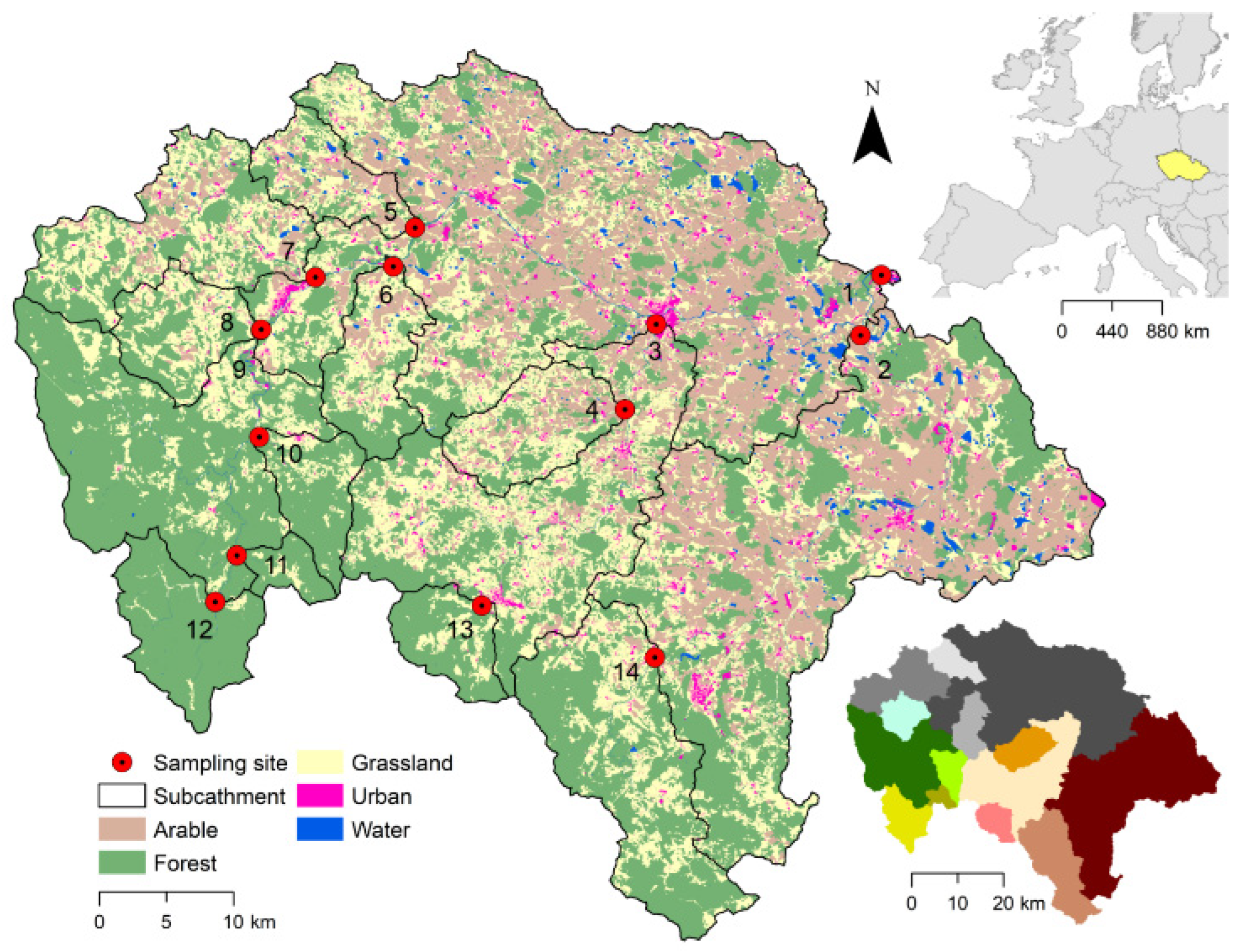
2.1. Study Site
2.2. Trends in Governing Pressures
2.3. Land Use and Other Catchment Characteristics
2.4. Biochemical Analysis
2.5. Derived Parameters and Statistical Analysis
3. Results and Discussions
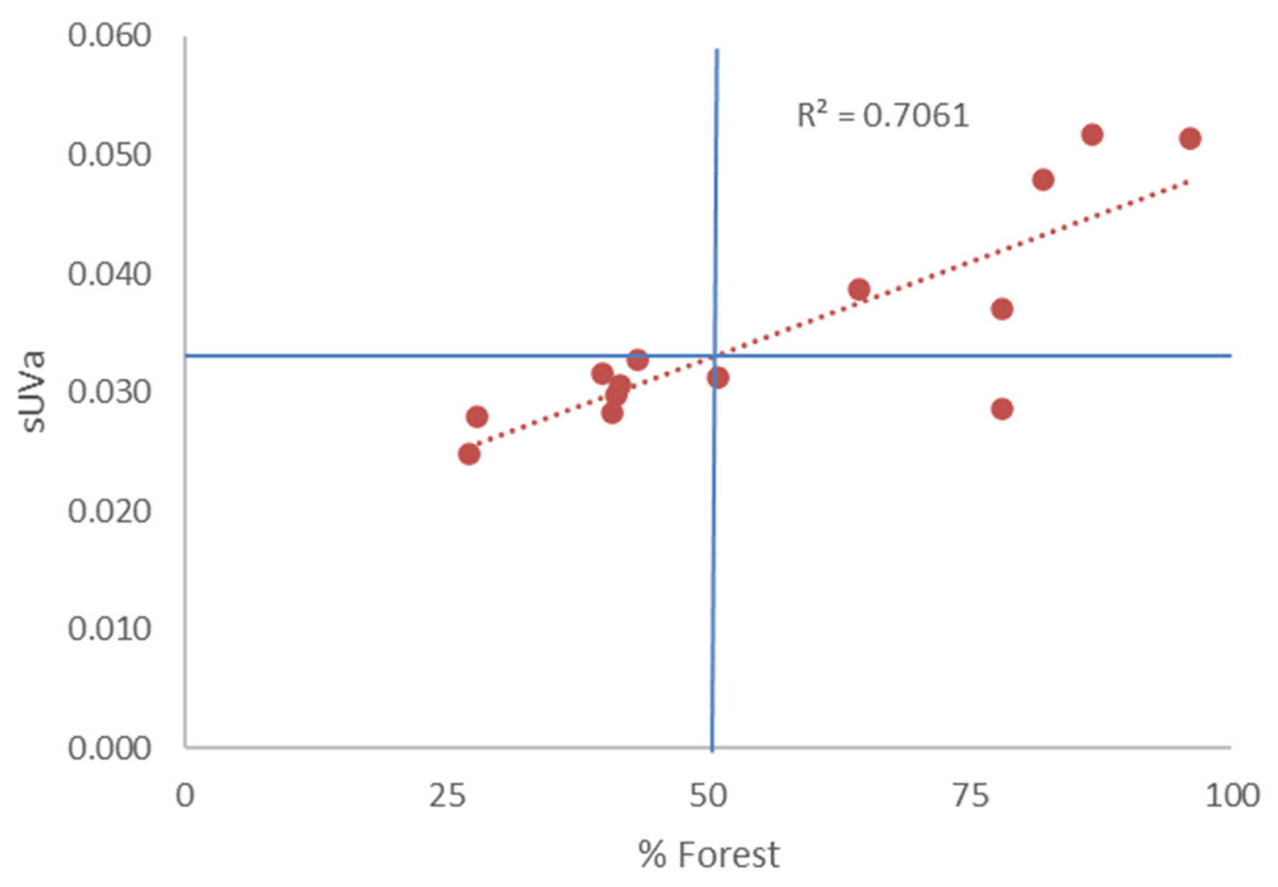
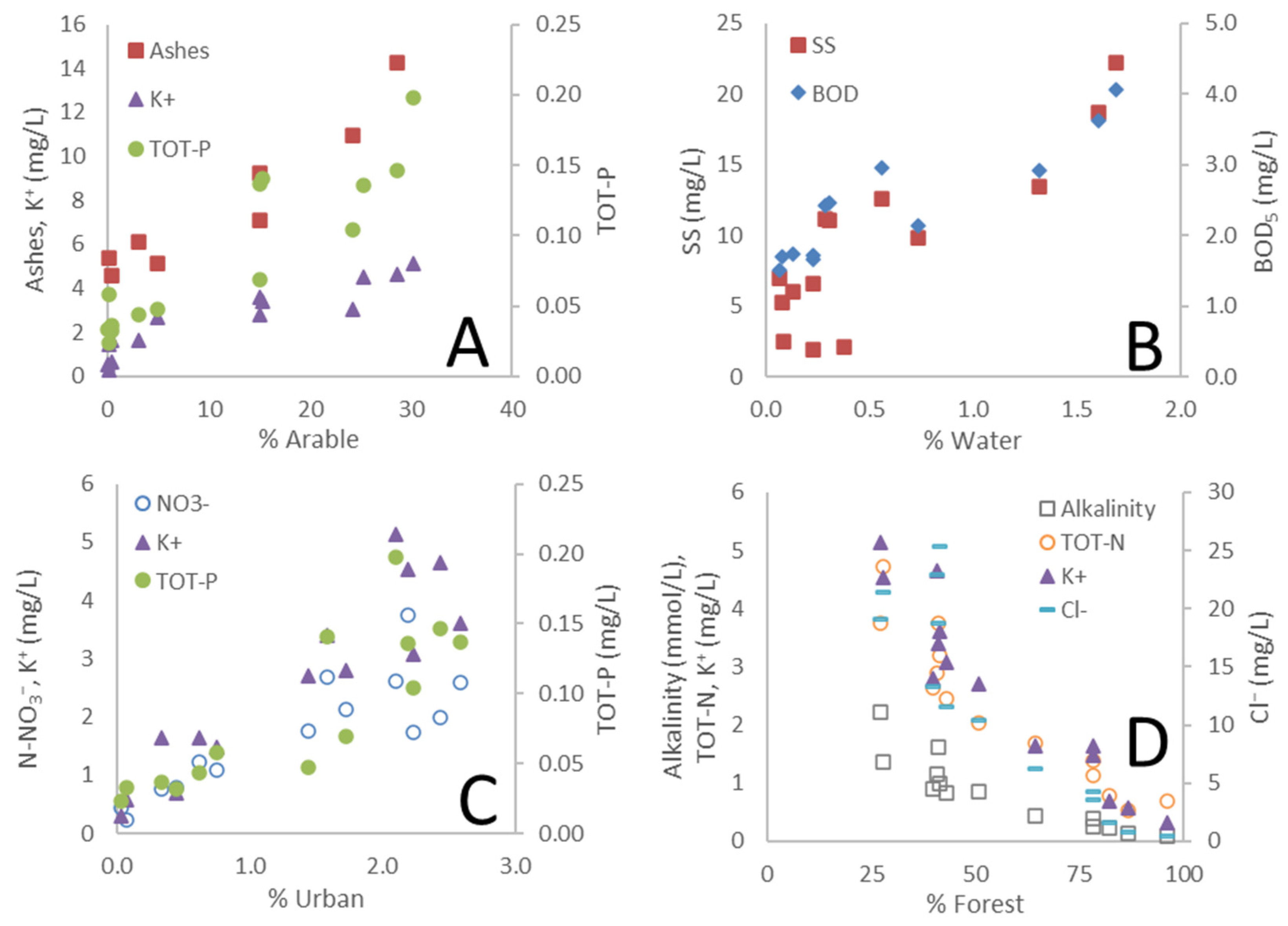
3.1. Land Use as a Governing Factor on Spatial Differences in Water Chemistry
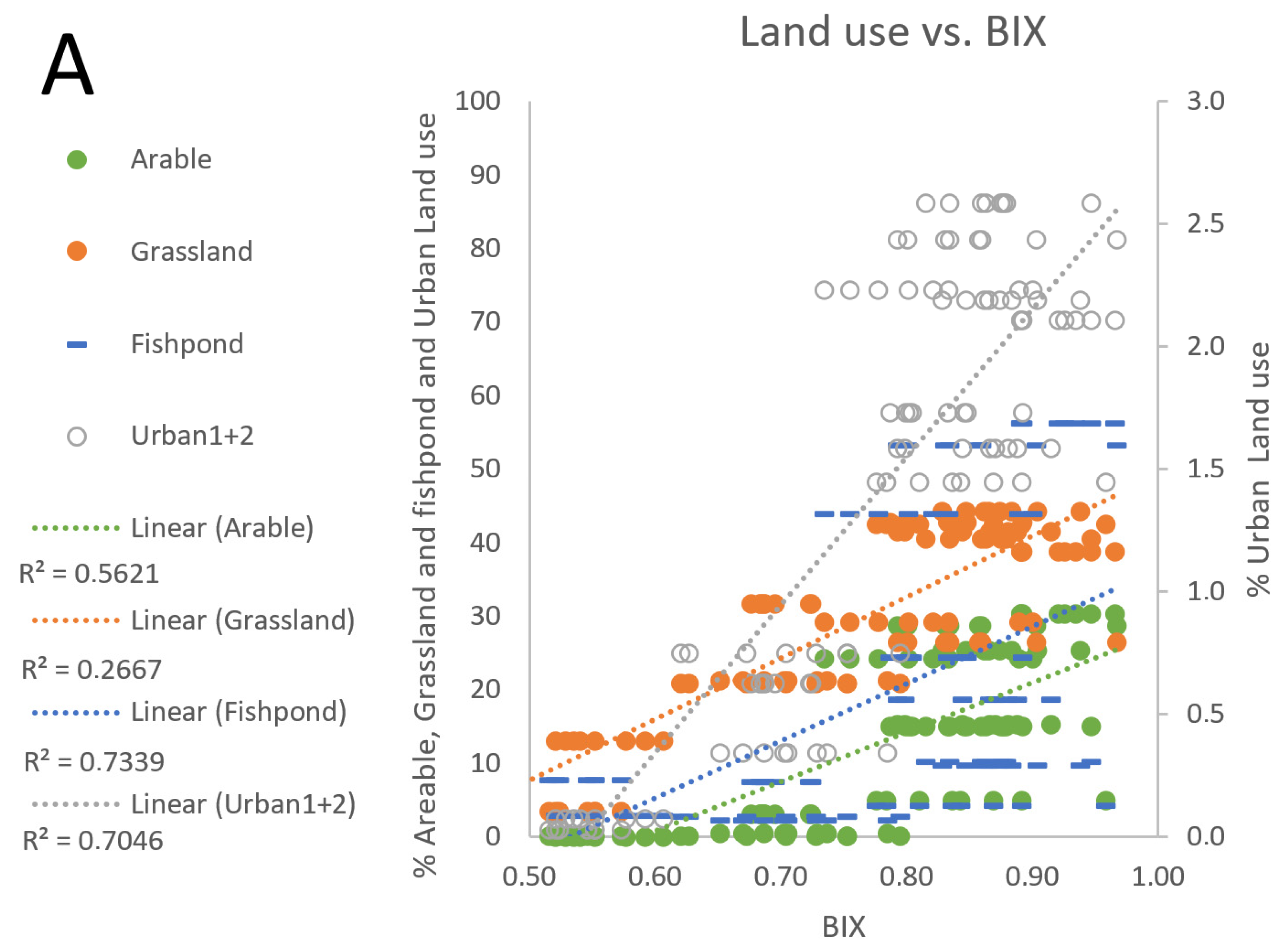
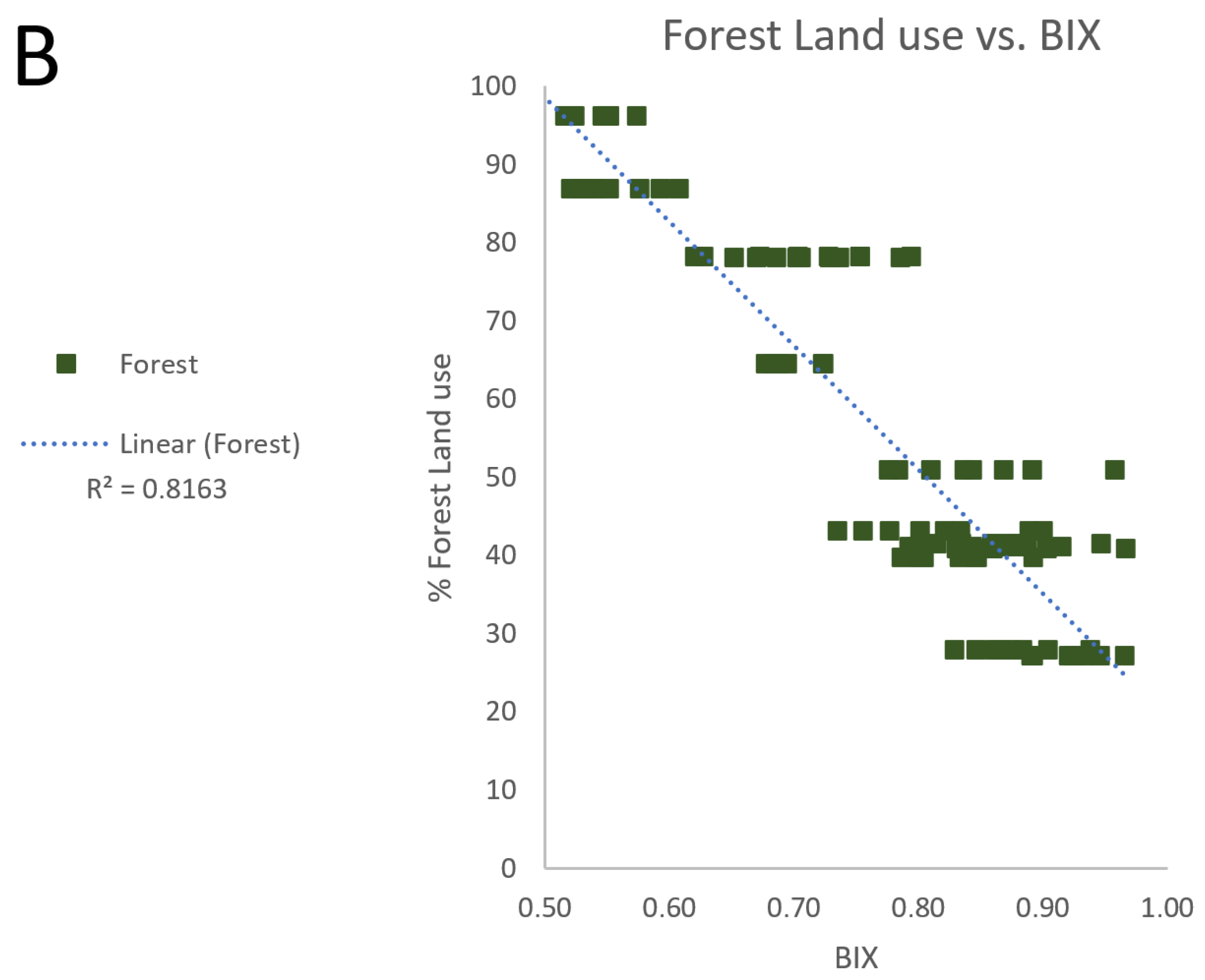
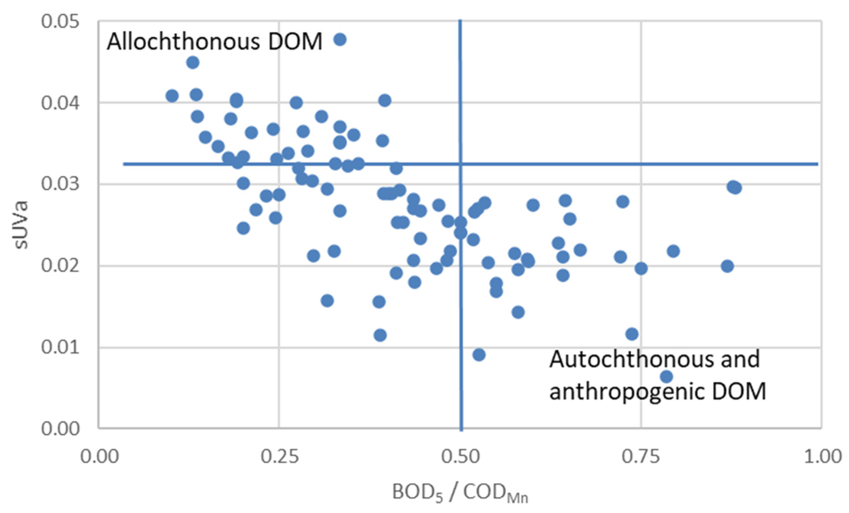
3.2. Governing Factors on DOM
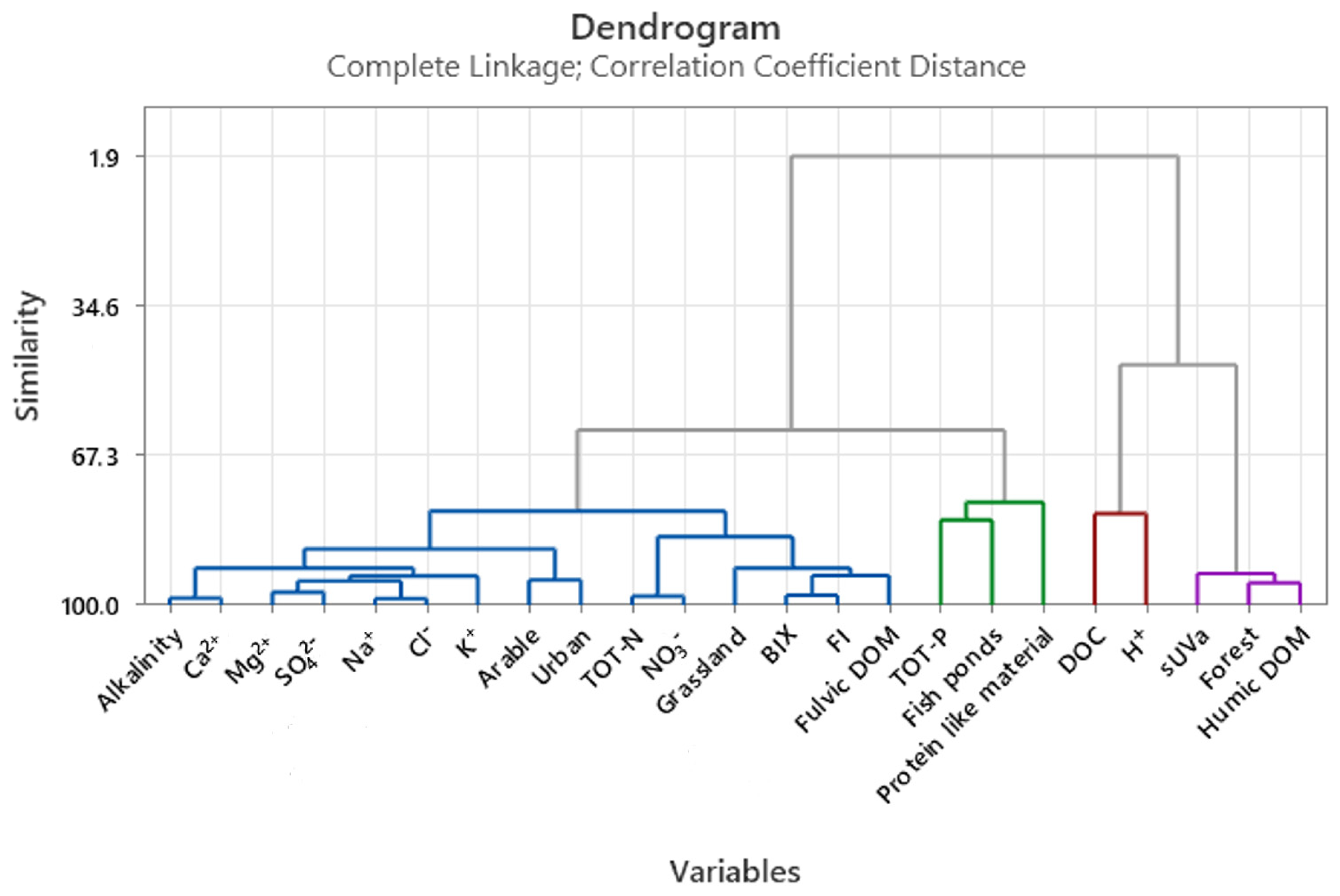
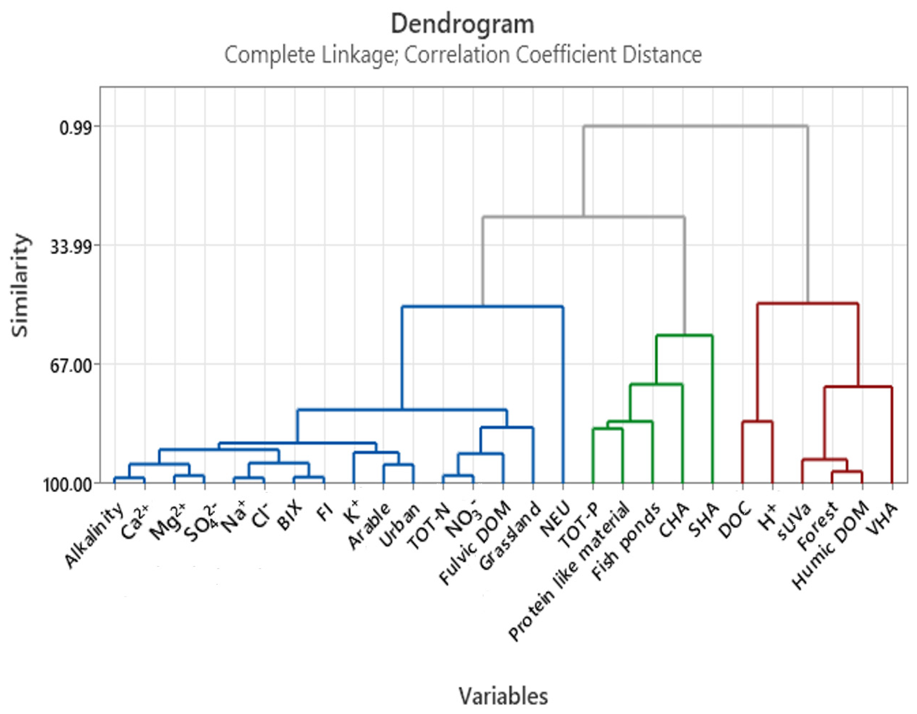
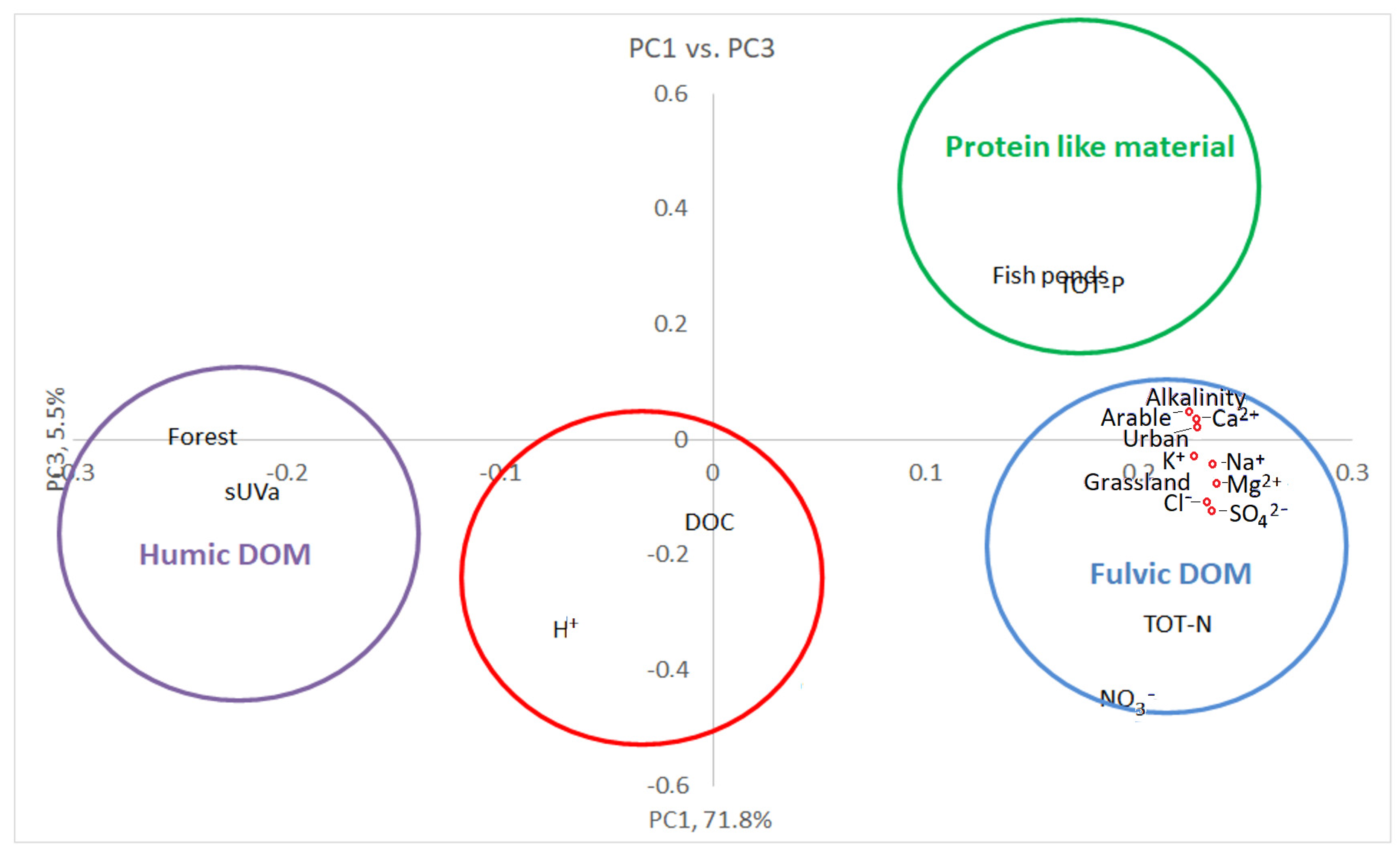
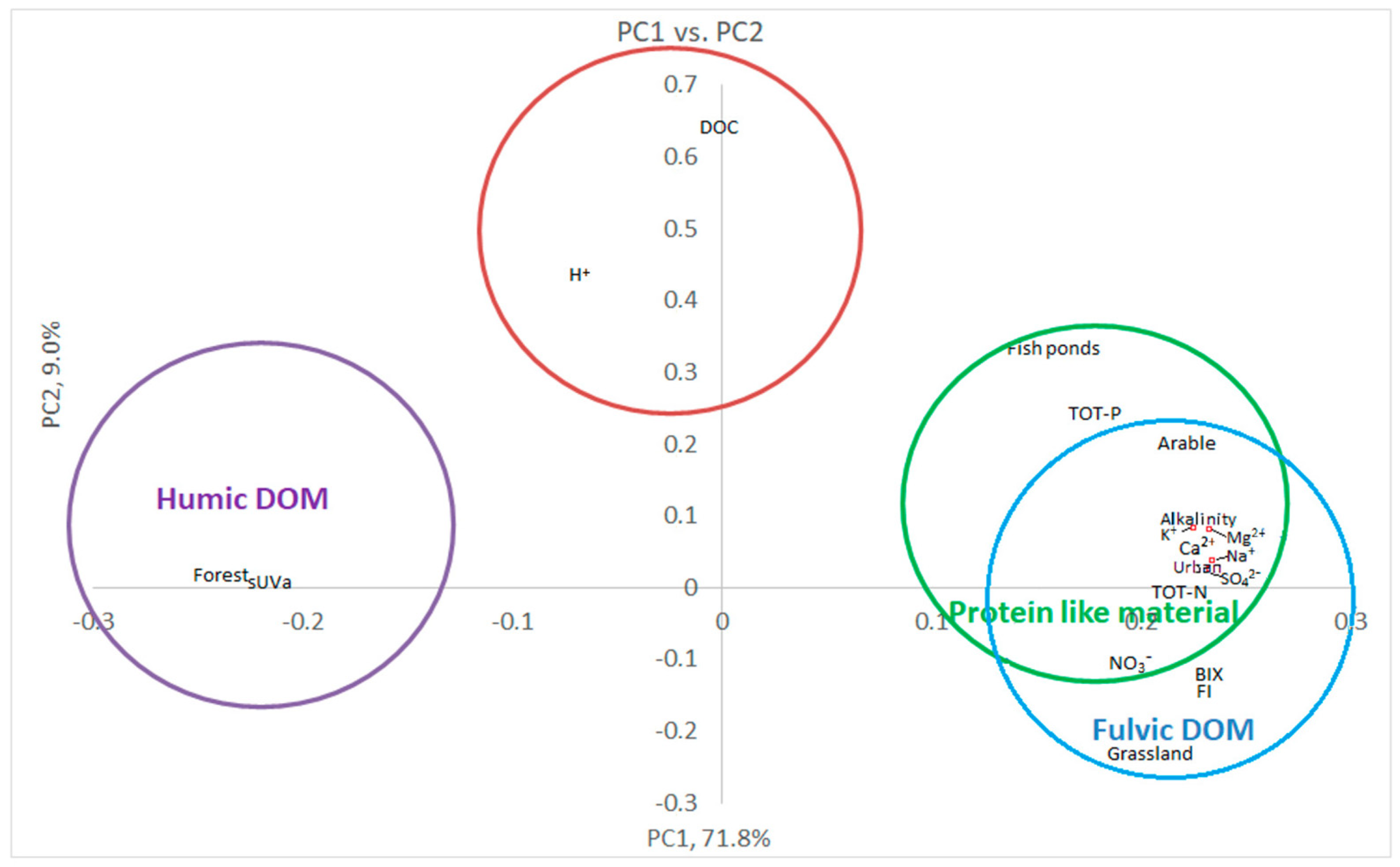
3.3. Multivariate Statistics
3.4. Fishpond Study
4. Conclusions
Author Contributions
Funding
Data Availability Statement
Conflicts of Interest
Appendix A

| Parameter | Method of Analysis/Instrument | Ref. |
|---|---|---|
| pH | Probe YSI 6600 V2-4 (Xylem Inc.) | - |
| Suspended solids (mg L−1) | Gravimetry after drying at 105 °C | [50] |
| Alkalinity | Titrimetric determination of acid neutralizing capacity to pH 4.5 (ANC4.5) | [51] |
| Biochemical oxygen demand after 5 days (BOD5, mg L−1) | Electrochemical or optical probe methods | [52] |
| Chemical oxygen demand by permanganate (CODMn, mg L−1) | Titrimetric determination after digestion with permanganate | [53] |
| Chemical oxygen demand by dichromate method (CODCr, mg L−1) | Spectrophotometric test tube method | [54] |
| UV absorbency (Abs. @UVλ254) | Spectrometry (Shimadzu UV-1650 PC) | [55] |
| TOT-P (mg L−1) | Inductive coupled plasma spectrometry (Agilent 8800 ICP-MSQ) | [56] |
| PO43− (mg L−1) | Spectrophotometric ammonium molybdate method (Shimadzu UV-1650 PC) | [57] |
| TOT-N (mg L−1) | High-temperature combustion (Multi N/C 2100 analyzer, Analytik Jena AG, Germany) with unfiltered water samples | [58] |
| N-NH4+ (mg L−1) | Spectrophotometry (Shimadzu UV-1650 PC) | [59] |
| SO42−, N-NO3−, Cl−, (mg L−1) | Ion chromatography (Dionex ICS-1000) | [60] |
| Ca2+, Mg2+, Na+, K+ (mg L−1) | Ion chromatography (Dionex ICS-1000) | [61] |
| Chl-a (µg L−1) | Spectrometry (Shimadzu UV-1650 PC) | [62] |
| TC (mg L−1) | High-temperature combustion method (Multi N/C 2100 analyzer, Analytik Jena AG, Germany) | [63] |
| TIC (mg L−1) | Low-temperature acidification method (Multi N/C 2100 analyzer, Analytik Jena AG, Germany) | [63] |
| TOC (mg L−1) | TOC = TC − TIC | [63] |
| DC (mg L−1) | High-temperature combustion method (Multi N/C 2100 analyzer, Analytik Jena AG, Germany) | [63] |
| DIC (mg L−1) | Low temperature acidification method (Multi N/C 2100 analyzer, Analytik Jena AG, Germany) | [63] |
| DOC (mg L−1) | DOC = DC − DIC | [63] |
| Parameter | Method of Analysis/Instrument | Ref. |
|---|---|---|
| pH | TIM865, Radiometer | - |
| Suspended solids (mg L−1) | Gravimetry after drying at 105 °C | [50] |
| Alkalinity | Titrimetric determination of acid neutralizing capacity according to Gran using TIM865, Radiometer | [51] |
| UV absorbency (Abs. @UVλ254) | Spectrometry (Shimadzu UV-2700) | [55] |
| TOT-P (mg L−1) | Spectrophotometric molybdate method (Kopáček and Hejzlar, 1993) | [57] |
| PO43− (mg L−1) | Spectrophotometric ammonium molybdate method (Specord 50, Analytik Jena) Murphy and Riley (1962) | [57] |
| Tot-N (mg L−1) | High-temperature combustion (Shimadzu TOC-L) with unfiltered water samples | [58] |
| N-NH4+ (mg L−1) | Spectrophotometry (Specord 50, Analytik Jena) | [59] |
| N-NO3−, Cl−, SO42− (mg L−1) | Ion chromatography (Dionex ICS-5000+) | [60] |
| Ca2+, Mg2+, Na+, K+ (mg L−1) | Ion chromatography (Dionex IC25) | [61] |
| TOC (mg L−1) | Nonpurgable total organic carbon (Shimadzu TOC-5000A) | [63] |
| DOC (mg L−1) | Nonpurgable dissolved organic carbon (Shimadzu TOC-L) | [63] |
Appendix B
| Site | pH | Alkalinity | SS | TOT-N | TOT-P | Ca2+ | Mg2+ | Na+ | K+ | SO42− | NO3− | Cl− | PO43− | N-NH4+ |
|---|---|---|---|---|---|---|---|---|---|---|---|---|---|---|
| # | mmol L−1 | mg L−1 | mg L−1 | mg L−1 | mg L−1 | mg L−1 | mg L−1 | mg L−1 | mg L−1 | mg L−1 | mg L−1 | mg L−1 | mg L−1 | |
| 1 | 7.53 | 0.83 | 13.5 | 2.45 | 0.10 | 14.5 | 5.60 | 7.51 | 3.07 | 22.2 | 1.73 | 11.6 | 0.05 | 0.09 |
| 2 | 7.45 | 1.14 | 18.7 | 2.89 | 0.15 | 24.1 | 8.83 | 15.1 | 4.65 | 33.3 | 1.99 | 22.9 | 0.05 | 0.11 |
| 3 | 7.58 | 0.99 | 11.1 | 3.19 | 0.14 | 22.5 | 7.06 | 14.9 | 3.61 | 24.7 | 2.60 | 25.4 | 0.09 | 0.08 |
| 4 | 7.51 | 1.36 | 11.2 | 4.71 | 0.14 | 28.5 | 9.88 | 13.6 | 4.54 | 35.4 | 3.74 | 21.4 | 0.10 | 0.09 |
| 5 | 7.80 | 2.23 | 22.2 | 3.75 | 0.20 | 40.3 | 14.2 | 15.5 | 5.13 | 44.8 | 2.61 | 19.1 | 0.09 | 0.14 |
| 6 | 7.76 | 1.61 | 12.6 | 3.74 | 0.14 | 35.3 | 9.38 | 11.5 | 3.41 | 29.4 | 2.67 | 18.7 | 0.10 | 0.28 |
| 7 | 7.45 | 0.89 | 9.85 | 2.63 | 0.07 | 14.9 | 6.17 | 8.72 | 2.80 | 21.1 | 2.14 | 13.4 | 0.03 | 0.06 |
| 8 | 7.53 | 0.85 | 5.99 | 2.04 | 0.05 | 18.3 | 4.59 | 7.50 | 2.71 | 17.4 | 1.75 | 10.4 | 0.02 | 0.04 |
| 9 | 7.00 | 0.22 | 2.10 | 0.78 | 0.03 | 3.80 | 1.00 | 2.59 | 0.69 | 4.41 | 0.78 | 1.64 | 0.02 | 0.01 |
| 10 | 7.18 | 0.39 | 5.25 | 1.38 | 0.06 | 8.58 | 2.41 | 4.30 | 1.49 | 11.4 | 1.08 | 4.28 | 0.04 | 0.04 |
| 11 | 6.57 | 0.12 | 2.54 | 0.52 | 0.03 | 1.84 | 0.53 | 2.03 | 0.57 | 3.05 | 0.24 | 0.75 | 0.02 | 0.00 |
| 12 | 5.72 | 0.10 | 1.92 | 0.68 | 0.02 | 1.47 | 0.43 | 1.43 | 0.31 | 1.45 | 0.44 | 0.41 | 0.01 | 0.03 |
| 13 | 7.14 | 0.26 | 7.03 | 1.13 | 0.04 | 2.78 | 1.71 | 4.38 | 1.63 | 12.0 | 0.76 | 3.57 | 0.01 | 0.02 |
| 14 | 7.45 | 0.44 | 6.64 | 1.68 | 0.04 | 6.28 | 3.99 | 13.4 | 1.66 | 12.4 | 1.23 | 6.19 | 0.02 | 0.03 |
| STD | STD | STD | STD | STD | STD | STD | STD | STD | STD | STD | STD | STD | STD | |
| 1 | 0.02 | 0.23 | 24.2 | 1.04 | 0.05 | 5.37 | 2.09 | 2.36 | 1.01 | 6.98 | 0.92 | 4.03 | 0.03 | 0.07 |
| 2 | 0.02 | 0.24 | 17.3 | 1.26 | 0.07 | 4.59 | 1.32 | 3.09 | 1.50 | 6.72 | 1.16 | 5.21 | 0.03 | 0.10 |
| 3 | 0.01 | 0.09 | 20.8 | 0.92 | 0.07 | 3.95 | 0.85 | 1.58 | 0.78 | 4.27 | 0.78 | 3.86 | 0.04 | 0.08 |
| 4 | 0.03 | 0.17 | 15.6 | 1.30 | 0.09 | 4.95 | 1.03 | 1.15 | 0.87 | 6.50 | 1.34 | 2.99 | 0.06 | 0.14 |
| 5 | 0.01 | 0.31 | 65.1 | 1.76 | 0.12 | 8.29 | 1.85 | 1.48 | 1.23 | 12.5 | 1.62 | 4.40 | 0.07 | 0.22 |
| 6 | 0.02 | 0.23 | 9.11 | 0.83 | 0.08 | 4.79 | 1.34 | 1.12 | 0.75 | 5.53 | 0.92 | 3.57 | 0.06 | 0.17 |
| 7 | 0.02 | 0.11 | 13.6 | 0.93 | 0.03 | 5.50 | 1.87 | 0.53 | 0.59 | 4.69 | 0.83 | 2.00 | 0.02 | 0.04 |
| 8 | 0.02 | 0.09 | 7.85 | 0.57 | 0.02 | 3.11 | 0.38 | 1.23 | 0.69 | 2.11 | 0.50 | 3.03 | 0.01 | 0.05 |
| 9 | 0.21 | 0.05 | 1.38 | 0.08 | 0.01 | 0.52 | 0.18 | 0.40 | 0.16 | 0.94 | 0.88 | 0.47 | 0.01 | 0.01 |
| 10 | 0.05 | 0.04 | 8.51 | 0.39 | 0.03 | 1.21 | 0.47 | 0.51 | 0.33 | 1.76 | 0.30 | 1.16 | 0.02 | 0.06 |
| 11 | 0.19 | 0.02 | 2.17 | 0.09 | 0.01 | 0.35 | 0.12 | 0.30 | 0.16 | 0.61 | 0.09 | 0.14 | 0.01 | 0.00 |
| 12 | 4.58 | 0.03 | 0.69 | 0.14 | 0.01 | 0.38 | 0.15 | 0.38 | 0.11 | 0.35 | 0.13 | 0.08 | 0.01 | 0.01 |
| 13 | 0.27 | 0.11 | 18.1 | 0.55 | 0.04 | 1.79 | 0.72 | 1.85 | 0.33 | 3.01 | 0.30 | 2.91 | 0.01 | 0.02 |
| 14 | 0.02 | 0.09 | 14.9 | 0.65 | 0.03 | 2.75 | 1.37 | 5.14 | 0.43 | 2.34 | 0.51 | 1.87 | 0.01 | 0.04 |
| # | # | # | # | # | # | # | # | # | # | # | # | # | # | |
| 1 | 246 | 125 | 257 | 245 | 256 | 126 | 126 | 102 | 8 | 126 | 257 | 126 | 257 | 257 |
| 2 | 182 | 8 | 183 | 171 | 183 | 8 | 8 | 8 | 8 | 8 | 183 | 8 | 183 | 182 |
| 3 | 185 | 11 | 185 | 173 | 185 | 8 | 8 | 8 | 8 | 8 | 185 | 8 | 185 | 185 |
| 4 | 183 | 8 | 65 | 53 | 183 | 8 | 8 | 8 | 8 | 8 | 183 | 8 | 90 | 183 |
| 5 | 255 | 8 | 232 | 233 | 256 | 8 | 8 | 8 | 8 | 103 | 256 | 103 | 199 | 256 |
| 6 | 179 | 8 | 81 | 69 | 199 | 8 | 8 | 8 | 8 | 23 | 190 | 23 | 90 | 190 |
| 7 | 211 | 8 | 221 | 211 | 223 | 28 | 28 | 8 | 8 | 8 | 223 | 8 | 221 | 221 |
| 8 | 176 | 8 | 176 | 176 | 164 | 8 | 8 | 8 | 8 | 8 | 176 | 8 | 176 | 175 |
| 9 | 55 | 54 | 8 | 8 | 8 | 8 | 8 | 8 | 8 | 9 | 9 | 8 | 8 | 7 |
| 10 | 222 | 8 | 234 | 222 | 234 | 8 | 8 | 8 | 8 | 8 | 234 | 8 | 234 | 229 |
| 11 | 8 | 8 | 8 | 8 | 8 | 8 | 8 | 8 | 8 | 8 | 8 | 8 | 8 | 4 |
| 12 | 68 | 8 | 73 | 68 | 73 | 8 | 8 | 8 | 8 | 8 | 73 | 8 | 73 | 70 |
| 13 | 259 | 116 | 259 | 247 | 259 | 116 | 116 | 104 | 8 | 116 | 259 | 116 | 259 | 254 |
| 14 | 259 | 32 | 259 | 247 | 259 | 32 | 32 | 32 | 8 | 7 | 258 | 31 | 259 | 253 |
| Sort | DOC | sUVa | BOD5 | CODCr | CODMn | Chl-a | BIX | FI | HIX | VHA | SHA | CHA | NEU | HPO | HPI |
|---|---|---|---|---|---|---|---|---|---|---|---|---|---|---|---|
| # | mg L−1 | cm−1/ mg C/L) | mg L−1 | mg L−1 | mg L−1 | mg L−1 | % | % | % | % | % | % | |||
| 1 | 6.94 | 0.033 | 2.92 | 21.0 | 7.65 | 13.6 | 0.81 | 1.29 | 0.84 | 71.1 | 2.72 | 4.59 | 21.6 | 73.8 | 26.21 |
| 2 | 9.52 | 0.028 | 3.62 | 25.7 | 7.32 | 44.1 | 0.86 | 1.33 | 0.84 | 69.4 | 7.16 | 4.80 | 18.6 | 76.6 | 23.4 |
| 3 | 4.87 | 0.031 | 2.47 | 16.2 | 4.73 | 6.05 | 0.87 | 1.34 | 0.85 | 69.0 | 3.92 | 0.79 | 26.3 | 73.0 | 27.0 |
| 4 | 6.44 | 0.028 | 2.43 | 19.2 | 5.99 | 9.83 | 0.88 | 1.37 | 0.88 | 69.3 | 5.21 | 5.88 | 19.9 | 74.5 | 25.5 |
| 5 | 8.77 | 0.025 | 4.07 | 28.7 | 8.44 | 22.1 | 0.92 | 1.38 | 0.84 | 58.2 | 16.3 | 8.47 | 17.0 | 74.5 | 25.5 |
| 6 | 4.78 | 0.030 | 2.96 | 17.3 | - | 6.21 | 0.86 | 1.33 | 0.85 | 60.5 | 11.4 | 4.05 | 24.0 | 71.9 | 28.1 |
| 7 | 5.43 | 0.032 | 2.13 | 13.4 | 4.26 | 3.39 | 0.83 | 1.33 | 0.84 | 63.2 | 11.2 | 0.96 | 24.6 | 74.5 | 25.5 |
| 8 | 2.60 | 0.031 | 1.74 | 8.68 | 2.93 | 3.28 | 0.85 | 1.32 | 0.82 | 54.0 | 13.4 | 0.00 | 32.6 | 67.4 | 32.6 |
| 9 | 5.25 | 0.048 | - | - | 6.47 | - | 0.60 | 1.11 | 0.86 | 77.9 | 5.38 | 1.13 | 15.6 | 83.3 | 16.7 |
| 10 | 3.59 | 0.029 | 1.70 | 10.3 | 3.87 | - | 0.71 | 1.20 | 0.84 | 67.7 | 3.28 | 1.25 | 27.8 | 71.0 | 29.0 |
| 11 | 7.03 | 0.052 | - | - | - | - | 0.56 | 1.10 | 0.87 | 80.2 | 4.53 | 0.72 | 14.6 | 84.7 | 15.3 |
| 12 | 9.49 | 0.051 | 1.66 | 26.3 | 12.6 | - | 0.53 | 1.07 | 0.87 | 81.5 | 6.45 | 1.60 | 10.4 | 88.0 | 12.0 |
| 13 | 4.05 | 0.037 | 1.51 | 13.7 | 4.92 | - | 0.71 | 1.24 | 0.87 | 69.0 | 6.98 | 1.80 | 22.2 | 76.0 | 24.0 |
| 14 | 5.53 | 0.039 | 1.72 | 15.8 | 5.33 | 3.07 | 0.69 | 1.21 | 0.88 | 68.9 | 10.2 | 3.18 | 17.7 | 79.1 | 20.9 |
| STD | STD | STD | STD | STD | STD | STD | STD | STD | STD | STD | STD | STD | STD | STD | |
| 1 | 2.60 | 0.01 | 1.08 | 8.80 | 3.58 | 10.4 | 0.06 | 0.05 | 0.04 | 6.32 | 3.32 | 5.30 | 10.29 | 6.31 | 6.31 |
| 2 | 4.15 | 0.01 | 1.39 | 9.13 | 2.50 | 27.4 | 0.06 | 0.04 | 0.03 | 5.76 | 4.80 | 5.64 | 7.57 | 5.40 | 5.40 |
| 3 | 1.22 | 0.00 | 1.33 | 8.22 | 1.82 | 7.28 | 0.04 | 0.03 | 0.03 | 3.31 | 7.84 | 1.59 | 7.23 | 5.73 | 5.73 |
| 4 | 1.49 | 0.00 | 1.39 | 9.00 | 1.83 | 7.01 | 0.04 | 0.03 | 0.02 | 6.97 | 7.02 | 4.50 | 6.62 | 7.43 | 7.43 |
| 5 | 2.16 | 0.00 | 2.25 | 22.5 | 2.86 | 20.4 | 0.03 | 0.03 | 0.03 | 3.59 | 3.22 | 3.87 | 5.30 | 3.89 | 3.89 |
| 6 | 1.18 | 0.00 | 1.50 | 6.58 | - | 7.40 | 0.04 | 0.03 | 0.03 | 4.35 | 8.20 | 5.06 | 11.9 | 7.32 | 7.32 |
| 7 | 1.98 | 0.00 | 0.83 | 7.16 | 2.36 | 3.21 | 0.03 | 0.04 | 0.06 | 2.01 | 7.79 | 1.11 | 9.56 | 8.69 | 8.69 |
| 8 | 0.94 | 0.00 | 0.70 | 4.09 | 1.75 | 1.65 | 0.06 | 0.06 | 0.06 | 8.52 | 9.90 | 0.00 | 12.9 | 12.9 | 12.9 |
| 9 | 3.18 | 0.00 | - | - | 4.43 | - | 0.04 | 0.04 | 0.07 | 6.18 | 4.72 | 2.27 | 5.24 | 3.81 | 3.81 |
| 10 | 1.52 | 0.01 | 0.91 | 6.56 | 2.51 | - | 0.06 | 0.04 | 0.07 | 12.1 | 4.12 | 2.49 | 15.2 | 13.3 | 13.3 |
| 11 | 5.69 | 0.00 | - | - | - | - | 0.03 | 0.03 | 0.05 | 10.1 | 2.65 | 0.52 | 10.8 | 10.5 | 10.5 |
| 12 | 5.84 | 0.00 | 0.72 | 14.4 | 7.07 | - | 0.03 | 0.02 | 0.05 | 6.45 | 3.12 | 1.87 | 9.87 | 9.32 | 9.32 |
| 13 | 2.35 | 0.00 | 1.09 | 14.7 | 4.08 | - | 0.04 | 0.04 | 0.04 | 7.40 | 4.82 | 3.61 | 14.7 | 11.7 | 11.7 |
| 14 | 2.53 | 0.00 | 0.97 | 9.41 | 3.15 | 3.64 | 0.02 | 0.03 | 0.03 | 3.77 | 7.28 | 3.72 | 7.38 | 6.34 | 6.34 |
| # | # | # | # | # | # | # | # | # | # | # | # | # | # | # | |
| 1 | 209 | 8 | 247 | 249 | 236 | 214 | 8 | 8 | 8 | 4 | 4 | 4 | 4 | 4 | 4 |
| 2 | 8 | 8 | 173 | 175 | 9 | 11 | 8 | 8 | 8 | 4 | 4 | 4 | 4 | 4 | 4 |
| 3 | 8 | 8 | 176 | 177 | 45 | 132 | 8 | 8 | 8 | 4 | 4 | 4 | 4 | 4 | 4 |
| 4 | 8 | 8 | 165 | 175 | 45 | 29 | 8 | 8 | 8 | 4 | 4 | 4 | 4 | 4 | 4 |
| 5 | 8 | 8 | 247 | 248 | 120 | 29 | 8 | 8 | 8 | 4 | 4 | 4 | 4 | 4 | 4 |
| 6 | 8 | 8 | 145 | 182 | 0 | 29 | 8 | 8 | 8 | 4 | 4 | 4 | 4 | 4 | 4 |
| 7 | 18 | 8 | 213 | 215 | 96 | 40 | 8 | 8 | 8 | 4 | 4 | 4 | 4 | 4 | 4 |
| 8 | 8 | 8 | 167 | 168 | 96 | 6 | 8 | 8 | 8 | 4 | 4 | 4 | 4 | 4 | 4 |
| 9 | 9 | 8 | 0 | 0 | 47 | 0 | 8 | 8 | 8 | 4 | 4 | 4 | 4 | 4 | 4 |
| 10 | 78 | 114 | 223 | 226 | 213 | 0 | 8 | 8 | 8 | 4 | 4 | 4 | 4 | 4 | 4 |
| 11 | 8 | 8 | 0 | 0 | 0 | 0 | 8 | 8 | 8 | 4 | 4 | 4 | 4 | 4 | 4 |
| 12 | 49 | 8 | 65 | 65 | 59 | 0 | 8 | 8 | 8 | 4 | 4 | 4 | 4 | 4 | 4 |
| 13 | 92 | 7 | 249 | 251 | 238 | 0 | 8 | 8 | 8 | 4 | 4 | 4 | 4 | 4 | 4 |
| 14 | 104 | 8 | 250 | 251 | 120 | 84 | 8 | 8 | 8 | 4 | 4 | 4 | 4 | 4 | 4 |
Appendix C


| Ref. | Component Assignment and Description | Location | Sample Type | Excitation/Emission Similarity Score | |
|---|---|---|---|---|---|
| Component 1: λexcitation, max/λemission, max = 265 (365)/487 | |||||
| 1 | [43] RaskaDOM | C2: Humic-like; large-sized; characteristics of soil, sediment, and freshwater environments. | Cropping system, Montana, USA | Soil water extractable DOM | 0.9920/0.9946 |
| 2 | [64] Wheat | C2: Humic-like; large-sized; characteristics of soil, sediment, and freshwater environments. | Cropping system, Montana, USA | Soil water extractable DOM | 0.9876/0.9972 |
| 3 | [65] Recycle | C1: Terrestrial humic-like fluorescence in high nutrient and wastewater-impacted environments. | Water recycling plant, Australia | Water recycling DOM | 0.9808/0.9986 |
| 4 | [66] Galveston bay | C1: similar to Coble peak C; humic-like. | Texas, USA | Riverine/Estuarine DOM | 0.9802/0.9975 |
| 5 | [67] Gueguen_Nelson | C1: Humic-like; terrestrially derived; Coble peak C; some photobleaching. | Beaufort Sea, experiments | Estuarine DOM | 0.9792/0.9933 |
| 6 | [68] Macaronesia | C3: humic-like. | Sao Vicente, Cape Verde, to Gran Canaria, Canary Island | Marine DOM | 0.9753/0.9968 |
| 7 | [69] | C1: Coble peak C+A; Humic-like; terrestrially derived. | Australia | Water treatment plant DOM | 0.9723/0.9988 |
| 8 | [43] | C2: humic-like; terrestrially derived material identified in a variety of aquatic environments; photosensitive. | Various freshwater environments across Quebec, Canada | Boreal freshwater DOM | 0.9965/0.9728 |
| 9 | [40] | C1: terrestrial and marine DOM. | Fjordsystem, Norway | Experimental marine DOM | 0.9798/0.9861 |
| 10 | [41] | C2: aromatic; high molecular weight organic matter (humic-like) with terrestrial character and correlated to lignin phenol concentrations; humic-like substance, enriched in terrestrial DOM sources; ubiquitous in DOM. | Experiments | SRHA DOM standard from the International Humic Substances Society | 0.9832/0.9724 |
| Component 2: λexcitation, max/λemission, max = 250 305/413 | |||||
| 1 | [70] | C4: UVA humic-like component frequently found in lentic freshwater; associated with bacterial planktonic activity. | The Sau Reservoir and its tributary the Ter River, Spain | Freshwater DOM | 0.9823/0.9924 |
| 2 | [41] | C3: combined Coble peaks A+M; microbial humic-like substances; produced by microbial degradation of organic matter. | Experiments | SRHA DOM standard from the International Humic Substances Society | 0.9887/0.9842 |
| 3 | [67] | C2: Humic-like; terrestrially derived; Coble peak A; susceptible to photobleaching. | Beaufort Sea, experiments | Estuarine DOM | 0.9790/0.9898 |
| 4 | [44] | C2: humic-like, ubiquitous humic component related with fulvic acids and re-processed humics. | Montseny Natural Park, Spain | Headwater forested catchment freshwater DOM | 0.9717/0.9968 |
| 5 | [45] | C1: terrestrial humic-like, microbial-humic-like. | The Baltimore sewer system, Baltimore, USA | Wastewater DOM | 0.9810/0.9865 |
| 6 | [66] Galveston bay | C2: similar to Coble peak M. | Texas, USA | Riverine/Estuarine DOM | 0.9834/0.9826 |
| 7 | [69] | C2: Coble peaks C+A; humic-like; terrestrial delivered reprocessed OM. | Australia | Water treatment plant DOM | 0.9733/0.9886 |
| 8 | [43] | C1: Humic-like; medium sized; characteristics of soil, sediment, and freshwater environments. | Cropping system, Montana, USA | Soil water extractable DOM | 0.9718/0.9548 |
| 9 | [64] | C2: Humic-like; medium sized; characteristics of soil, sediment, and freshwater environments. | Cropping system, Montana, USA | Soil water extractable DOM | 0.9826/0.9761 |
| 10 | [65] | C2: Microbial humic-like. | Water recycling plant, Australia | Water recycling DOM | 0.9826/0.9679 |
| Component 3: λexcitation, max/λemission, max = 280/336 | |||||
| 1 | [71] | C7: Protein-like; both tyrosine- and tryptophan-like properties. | Southern Onterio, Canada | Stormwater pond DOM | 0.9951/0.9961 |
| 2 | [72] | C5: Coble peak T; tryptophan-like. | Mackenzie, Lena, Kolyma, Ob, and Yenisei Rivers | Arctic river DOM | 0.9878/0.9947 |
| 3 | [73] | C5: Coble T peak; protein-like/tryptophan-like material with a recent, probably microbial origin. | Drinking water treatment plant, Sweden | Drinking water treatment plant water DOM | 0.9935/0.9867 |
| 4 | [74] | C2: tryptophan-like; protein-like. | Maryland, USA | Leaf litter leachate | 0.9877/0.9924 |
| 5 | [69] | C4: Coble peaks T+B, protein-like; microbial delivered. | Australia | Water treatment plant DOM | 0.9885/0.9886 |
| 6 | [46] | C4: tryptophan-like and protein-like material; generally contributes the highest intensity peaks in wastewaters, even in treated effluents; indicates recent production; often found in anthropogenically affected watersheds. | Coastal drainage basins of Miami, FL, USA | Coastal DOM | 0.9913/0.9845 |
| 7 | [75] | C3: Protein-like; fresh production; biological production; higher in surface water layer. | Indian ocean | Marine DOM | 0.9978/0.9781 |
| 8 | [76] | C4: Tryptophan-like; both photodegraded and produced during photodegradation, depending on sample type. | Subtropical Minjiang watershed, China | Wastewater, leaf litter leachates, river water DOM | 0.9864/0.9836 |
| 9 | [42] | C6: Associated with freshly produced protein-like material; tryptophan-like; strongest predictor of BDOC. | Various freshwater environments across Quebec, Canada | Boreal freshwater DOM | 0.9663/0.9825 |
| 10 | [45] | C4: Tryptophan-like; wastewater indicator. | The Baltimore sewer system, Baltimore, USA | Wastewater DOM | 0.9953/0.9538 |
Appendix D


References
- Thurman, E.M. Organic Geochemistry of Natural Waters; Springer: Dordrecht, The Netherlands, 1985. [Google Scholar] [CrossRef]
- Chudoba, J.; Hejzlar, J.; Doležal, M. Microbial polymers in the aquatic environment—III. Isolation from river, potable and ground water and analysis. Water Res. 1986, 20, 1223–1227. [Google Scholar] [CrossRef]
- Perdue, E.M. Natural Organic matter. In Reference Module in Earth Systems and Environmental Sciences, from Encyclopedia of Inland Waters; Likens, G.E., Ed.; Elsevier: Amsterdam, The Netherlands, 2009. [Google Scholar] [CrossRef]
- Swyngedouw, E. Modernity and Hybridity: Nature, Regeneracionismo, and the Production of the Spanish Waterscape, 1890–1930. Ann. Assoc. Am. Geogr. 1999, 89, 443–465. [Google Scholar] [CrossRef]
- Scholz, R.W. Environmental Literacy in Science and Society; From Knowledge to Decisions; Cambridge University Press: Cambridge, UK, 2011. [Google Scholar]
- Moore, J.W. Capitalism in the Web of Life; Verso: London, UK, 2015. [Google Scholar]
- Bonneuil, C.; Fressoz, J.-B. The Shock of the Anthropocene; Verso: London, UK, 2017. [Google Scholar]
- Winter, K.B.; Lincoln, N.K.; Berkes, F. The Social-Ecological Keystone Concept: A Quantifiable Metaphor for Understanding the Structure, Function, and Resilience of a Biocultural System. Sustainability 2018, 10, 3294. [Google Scholar] [CrossRef]
- Hejzlar, J.; Chudoba, J. Microbial polymers in the aquatic environment—II. Isolation from biologically non-purified and purified municipal waste water and analysis. Water Res. 1986, 20, 1217–1221. [Google Scholar] [CrossRef]
- Monteith, D.T.; Stoddard, J.L.; Evans, C.D.; De Wit, H.A.; Forsius, M.; Høgåsen, T.; Wilander, A.; Skjelkvåle, B.L.; Jeffries, D.S.; Vuorenmaa, J.; et al. Dissolved organic carbon trends resulting from changes in atmospheric deposition chemistry. Nature 2007, 450, 537–540. [Google Scholar] [CrossRef] [PubMed]
- De Wit, H.A.; Mulder, J.; Hindar, A.; Hole, L. Long-term increase in dissolved organic carbon in streamwaters in Norway is response to reduced acid deposition. Environ. Sci. Technol. 2007, 41, 7706–7713. [Google Scholar] [CrossRef]
- Monteith, D.T.; Henrys, P.A.; Hruška, J.; de Wit, H.A.; Krám, P.; Moldan, F.; Posch, M.; Räike, A.; Stoddard, J.L.; Shilland, E.M.; et al. Long-term rise in riverine dissolved organic carbon concentration is predicted by electrolyte solubility theory. Sci. Adv. 2023, 9, eade3491. [Google Scholar] [CrossRef] [PubMed]
- Vogt, R.D.; de Wit, H.; Koponen, K. Case Study on Impacts of Large-Scale Re-/Afforestation on Ecosystem Services in Nordic Regions. Report Series Quantifying and Deploying Responsible Negative Emissions in Climate Resilient Pathways. Horizon 2020, Grant Agreement no. 869192. 2022. Available online: https://www.negemproject.eu/wp-content/uploads/2022/06/NEGEM_D3.6_Case-study-on-impacts-of-large-scale-re-afforestation-on-ecosystem-services-in-Nordic-regions.pdf (accessed on 17 August 2023).
- Kopáček, J.; Evans, C.D.; Hejzlar, J.; Kaňa, J.; Porcal, P.; Šantrůčková, H. Factors affecting the leaching of dissolved organic carbon after tree dieback in an unmanaged European mountain forest. Environ Sci. Technol. 2018, 52, 6291–6299. [Google Scholar] [CrossRef]
- De Wit, H.A.; Garmo, Ø.A.; Jackson-Blake, L.; Clayer, F.; Vogt, R.D.; Kaste, Ø.; Gundersen, C.B.; Guerrerro, J.L.; Hindar, A. Changing Water Chemistry in One Thousand Norwegian Lakes During Three Decades of Cleaner Air and Climate Change. Glob. Biogeochem. Cycles 2023, 37, e2022GB007509. [Google Scholar] [CrossRef]
- Madsen, H.; Lawrence, D.; Lang, M.; Martinkova, M.; Kjeldsen, T.R. Review of trend analysis and climate change projections of extreme precipitation and floods in Europe. J. Hydrol. 2014, 519, 3634–3650. [Google Scholar] [CrossRef]
- Grennfelt, P.; Engleryd, A.; Forsius, M.; Hov, Ø.; Rodhe, H.; Cowling, E. Acid rain and air pollution: 50 years of progress in environmental science and policy. Ambio 2020, 49, 849–864. [Google Scholar] [CrossRef]
- Schulte-Uebbing, L.; de Vries, W. Global-scale impacts of nitrogen deposition on tree carbon sequestration in tropical, temperate, and boreal forests: A meta-analysis. Glob. Chang. Biol. 2018, 24, 416–431. [Google Scholar] [CrossRef]
- Kaste, Ø.; Skarbøvik, E.; Vogt, R.D. Assessment of Parameters for Suspended Solids and Organic Matter Can Be Included in the Water Classification System (in Norwegian). NIVA-Rapport 7860. 2023. Available online: https://hdl.handle.net/11250/3067437 (accessed on 17 August 2023).
- Hansen, A.M.; Kraus, T.E.C.; Pellerin, B.A.; Fleck, J.A.; Downing, B.D.; Bergamaschi, B.A. Optical properties of dissolved organic matter (DOM): Effects of biological and photolytic degradation. Limnol. Oceanogr. 2016, 61, 1015–1032. [Google Scholar] [CrossRef]
- Sample, J.E.; Jackson-Blake, L.; Vogelsang, C.; Kaste, Ø.; Vogt, R.D. TEOTIL3: A coefficient-based export model for simulation of river inputs (in Norwegian). NIVA report. In Prep. 2023. Available online: https://niva.brage.unit.no/niva-xmlui/ (accessed on 17 August 2023).
- Zsolnay, A.; Baigar, E.; Jimenez, M.; Steinweg, B.; Saccomandi, F. Differentiating with fluorescence spectroscopy the sources of dissolved organic matter in soils subjected to drying. Chemosphere 1999, 38, 45–50. [Google Scholar] [CrossRef] [PubMed]
- Huguet, A.; Vacher, L.; Relexans, S.; Saubusse, S.; Froidefond, J.M.; Parlanti, E. Properties of fluorescent dissolved organic matter in the Gironde Estuary. Org. Geochem. 2009, 40, 706–719. [Google Scholar] [CrossRef]
- Murphy, K.R.; Stedmon, C.A.; Wenig, P.; Bro, R. OpenFluor– an online spectral library of auto-fluorescence by organic compounds in the environment. Anal. Methods 2014, 6, 658–661. [Google Scholar] [CrossRef]
- Xu, X.; Kang, J.; Shen, J.; Zhao, S.; Wang, B.; Zhang, X.; Chen, Z. EEM–PARAFAC characterization of dissolved organic matter and its relationship with disinfection by-products formation potential in drinking water sources of northeastern China. Sci. Total Environ. 2021, 774, 145297. [Google Scholar] [CrossRef]
- Vogt, R.D.; Akkanen, J.; Andersen, D.O.; Bruggemann, R.; Chatterjee, B.; Gjessing, E.; Kukkonen, J.V.K.; Larsen, H.E.; Luster, J.; Paul, A.; et al. Key site variables governing the functional characteristics of dissolved natural organic matter (DNOM) in Nordic forested catchments. Aquat. Sci. 2004, 66, 195–210. [Google Scholar] [CrossRef]
- Mykkelbost, T.C.; Vogt, R.D.; Seip, H.M.; Riise, G. Organic carbon fractionation applied to lake-and soil water at the HUMEX site. Environ. Int. 1995, 21, 849–859. [Google Scholar] [CrossRef]
- Kopáček, J.; Hejzlar, J.; Porcal, P.; Posh, M. Trends in riverine element fluxes: A chronicle of regional socio-economic changes. Water Res. 2017, 125, 374–383. [Google Scholar] [CrossRef]
- Veselý, J.; Hruška, J.; Norton, S.A.; Johnson, C.E. Trends in water chemistry of acidified Bohemian lakes from 1984 to 1995: I. Major solutes. Water Air Soil Pollut. 1998, 108, 107–127. [Google Scholar] [CrossRef]
- Carlson, M. Mapping of Causes for Increase in Dissolved Organic Matter in a Czech Watershed. Master Thesis, University of Oslo, Oslo, Norway, June 2021. Available online: https://www.duo.uio.no/handle/10852/93531 (accessed on 17 August 2023).
- Schmidt, S.I.; Hejzlar, J.; Kopáček, J.; Paule-Mercado, M.C.; Porcal, P.; Vystavna, Y.; Lanta, V. Forest damage and subsequent recovery alter the water composition in mountain lake catchments. Sci. Total Environ. 2022, 827, 154293. [Google Scholar] [CrossRef]
- Chow, C.W.K.; Fabris, R.; Drikas, M. A rapid fractionation technique to characterise natural organic matter for the optimisation of water treatment processes. J. Water Supply Res. Technol. AQUA 2004, 53, 85–92. [Google Scholar] [CrossRef]
- Ohno, T. Fluorescence Inner-Filtering Correction for Determining the Humification Index of Dissolved Organic Matter. Environ. Sci. Technol. 2002, 36, 742–746. [Google Scholar] [CrossRef]
- Fellman, J.B.; Hood, E.; Spencer, R.G.M. Fluorescence Spectroscopy Opens New Windows into Dissolved Organic Matter Dynamics in Freshwater Ecosystems: A Review. Limnol. Oceanogr. 2010, 55, 2452–2462. [Google Scholar] [CrossRef]
- Li, P.; Hur, J. Utilization of UV-Vis spectroscopy and related data analyses for dissolved organic matter (DOM) studies: A review. Critical Reviews in Environ. Sci. Technol. 2017, 47, 131–154. [Google Scholar] [CrossRef]
- McKnight, D.M.; Boyer, E.W.; Westerhoff, P.K.; Doran, P.T.; Kulbe, T.; Andersen, D.T. Spectrofluorometric Characterization of Dissolved Organic Matter for Indication of Precursor Organic Material and Aromaticity. Limnol. Oceanogr. 2001, 46, 38–48. [Google Scholar] [CrossRef]
- da Silva, M.P.; Sander de Carvalho, L.A.; Novo, E.; Jorge, D.S.F.; Barbosa, C.C.F. Use of optical absorption indices to assess seasonal variability of dissolved organic matter in Amazon floodplain lakes. Biogeosciences 2020, 17, 5355–5364. [Google Scholar] [CrossRef]
- Pucher, M.; Wünsch, U.; Weigelhofer, G.; Murphy, K.; Hein, T.; Graeber, D. staRdom: Versatile Software for Analyzing Spectroscopic Data of Dissolved Organic Matter in R’. Water 2019, 11, 2366. [Google Scholar] [CrossRef]
- R Core Team. R: A Language and Environment for Statistical Computing; R Foundation for Statistical Computing: Vienna, Austria, 2023; Available online: https://www.R-project.org/ (accessed on 15 July 2023).
- Stedmon, C.; Bro, R. Characterizing Dissolved Organic Matter Fluorescence with Parallel Factor Analysis: A Tutorial. Limnol. Oceanogr. 2008, 6, 572–579. [Google Scholar] [CrossRef]
- Du, Y.; Zhang, Q.; Liu, Z.; He, H.; Lürling, M.; Chen, M.; Zhang, Y. Composition of dissolved organic matter controls interactions with La and Al ions: Implications for phosphorus immobilization in eutrophic lakes. Environ. Pollut. 2019, 248, 36–47. [Google Scholar] [CrossRef] [PubMed]
- Lapierre, J.F.; del Giorgio, P.A. Partial coupling and differential regulation of biologically and photochemically labile dissolved organic carbon across boreal aquatic networks. Biogeosciences 2014, 11, 5969–5985. [Google Scholar] [CrossRef]
- Romero, C.M.; Engel, R.E.; D’Andrilli, J.; Miller, P.R.; Wallander, R. Compositional tracking of dissolved organic matter in semiarid wheat-based cropping systems using fluorescence EEMs-PARAFAC and absorbance spectroscopy. J. Arid. Environ. 2019, 167, 34–42. [Google Scholar] [CrossRef]
- Bernal, S.; Lupon, A.; Catalán, N.; Castelar, S.; Martí, E. Decoupling of dissolved organic matter patterns between stream and riparian groundwater in a headwater forested catchment. Hydrol. Earth Syst. Sci. 2018, 22, 1897–1910. [Google Scholar] [CrossRef]
- Batista-Andrade, J.A.; Diaz, E.; Iglesias Vega, D.; Hain, E.; Rose, M.R.; Blaney, L. Spatiotemporal analysis of fluorescent dissolved organic matter to identify the impacts of failing sewer infrastructure in urban streams. Water Res. 2023, 229, 119521. [Google Scholar] [CrossRef]
- Smith, M.A.; Kominoski, J.S.; Gaiser, E.E.; Price, R.M.; Troxler, T.G. Stormwater Runoff and Tidal Flooding Transform Dissolved Organic Matter Composition and Increase Bioavailability in Urban Coastal Ecosystems. J. Geohys. Res. B 2021, 126, e2020JG006146. [Google Scholar] [CrossRef]
- Eikebrokk, B.; Haaland, S.L.; Jarvis, P.; Riise, G.; Vogt, R.D.; Zahlsen, K. NOMiNOR: Natural Organic Matter in Drinking Waters within the Nordic Region. In Norsk Vann Report; Norwegian Water: Oslo, Norway, 2018; Volume 231, Available online: https://va-kompetanse.no/butikk/a-231-nominor-natural-organic-matter-in-drinking-waters-within-the-nordic-region-kun-digital/ (accessed on 17 August 2023).
- Crapart, C.; Andersen, T.; Hessen, D.O.; Valiente, N.; Vogt, R.D. Factors Governing Biodegradability of Dissolved Natural Organic Matter in Lake Water. Water 2021, 13, 2210. [Google Scholar] [CrossRef]
- Crapart, C.; Finstad, A.G.; Hessen, D.O.; Vogt, R.D.; Andersen, T. Spatial predictors and temporal forecast of total organic carbon levels in boreal lakes. Sci. Total Environ. 2023, 870, 161676. [Google Scholar] [CrossRef]
- ČSN EN 12880; Water Quality, Determination of Dry Residue and Water Content of Sludges and Sludge Products. Czech Office for Standards, Metrology and Testing: Prague, Czech Republic, 2000.
- ČSN EN ISO 9963-1; Water Quality. Determination of Alkanity. Part 1: Determination of Total and Composite Alkanity. Czech Office for Standards, Metrology and Testing: Prague, Czech Republic, 1995.
- ČSN EN ISO 5815-1; Water Quality—DETERMINATION of Biochemical Oxygen Demand After n Days (BODn)—Part 1: Dilution and Seeding Method with Allylthiourea Addition. Czech Office for Standards, Metrology and Testing: Prague, Czech Republic, 2020.
- ČSN EN ISO 8467; Water Quality—Determination of Chemical Oxygen Demand by Permanganate (CODMn). Czech Office for Standards, Metrology and Testing: Prague, Czech Republic, 1997.
- ČSN ISO 157085; Geometrical Product Specifications (GPS)—Surface Texture: Profile Method—Terms, Definitions and Surface Texture Parameters. Czech Office for Standards, Metrology and Testing: Prague, Czech Republic, 2008.
- ČSN 757360; Water Quality, Determination of Absorbance. Direct Measurement of Absorption of UV Radiation at Wavelength 254 nm. Czech Office for Standards, Metrology and Testing: Prague, Czech Republic, 2013.
- ISO 17294-2; Water Quality-Application of Inductively Coupled Plasma Mass Spectrometry (ICP-MS)-Part 2: Determination of 62 Elements. International Organization for Standardization (ISO): Geneva, Switzerland, 2003; Volume 2.
- ISO 6878; Water Quality—Determination of Phosphorus—Ammonium Molybdate Spectrometric Method. International Organization for Standardization (ISO): Geneva, Switzerland, 2004.
- DIN EN 12260; Water Quality. Determination of Nitrogen. Determination of Bound Nitrogen (TNb), following Oxidation to Nitrogen Oxides. Deutches Institut fur Normung: Berlin, Germany, 2003.
- ISO 7150-1; Water Quality-Determination of Ammonium. Part 1: Manual Spectrometric Method. International Organization for Standardization (ISO): Geneva, Switzerland, 1984.
- ISO10304-1; Water Quality-Determination of Dissolved Anions by Liquid Chromatography of Ions-Part 1: Determination of Bromide, Chloride, Fluoride, Nitrate, Nitrite, Phosphate and Sulfate. International Organization for Standardization (ISO): Geneva, Switzerland, 2007; Volume 1.
- ČSN EN ISO 14911; Water Quality—Determination of Dissolved Li+, Na+, NH4+, K+, Mn2+, Ca2+, Mg2+, Sr2+ and Ba2+ Using Ion Chromatography—Method for Water and Waste Water. Czech Office for Standards, Metrology and Testing: Prague, Czech Republic, 2000.
- ISO 10260; Water Quality, Measurement of Biochemical Parameters; Spectrometric Determination of Chlorophyll-a Concentration (ISO: 1992). International Organization for Standardization (ISO): Geneva, Switzerland, 1992.
- ISO 8245; Water Quality-Guidelines for the Determination of Total Organic Carbon (TOC) and Dissolved Organic Carbon (DOC). International Organization for Standardization (ISO): Geneva, Switzerland, 1999.
- Romero, C.M.; Engel, R.E.; D’Andrilli, J.; Chen, C.; Zabinski, C.; Miller, P.R.; Wallander, R. Bulk optical characterization of dissolved organic matter from semiarid wheat-based cropping systems. Geoderma 2017, 306, 40–49. [Google Scholar] [CrossRef]
- Murphy, K.R.; Stedmon, C.A.; Graeber, D.; Bro, R. Fluorescence spectroscopy and multi-way techniques. PARAFAC. Anal. Methods 2013, 5, 6557–6566. [Google Scholar] [CrossRef]
- Gold-Bouchot, G.; Polis, S.; Castañon, L.E.; Flores, M.P.; Alsante, A.N.; Thornton, D.C.O. Chromophoric dissolved organic matter (CDOM) in a subtropical estuary (Galveston Bay, USA) and the impact of Hurricane Harvey. Environ. Sci. Pollut. Res. 2021, 28, 53045–53057. [Google Scholar] [CrossRef]
- Guéguen, C.; Mokhtar, M.; Perroud, A.; McCullough, G.; Papakyriakou, T. Mixing and photoreactivity of dissolved organic matter in the Nelson/Hayes estuarine system (Hudson Bay, Canada). J. Mar. Syst. 2016, 161, 42–48. [Google Scholar] [CrossRef]
- Santana-Casiano, J.M.; González-Santana, D.; Devresse, Q.; Hepach, H.; Santana-González, C.; Quack, B.; Engel, A.; González-Dávila, M. Exploring the Effects of Organic Matter Characteristics on Fe(II) Oxidation Kinetics in Coastal Seawater. Environ. Sci. Technol. 2022, 56, 2718–2728. [Google Scholar] [CrossRef] [PubMed]
- Shutova, Y.; Baker, A.; Bridgeman, J.; Henderson, R.K. Spectroscopic characterisation of dissolved organic matter changes in drinking water treatment: From PARAFAC analysis to online monitoring wavelengths. Water Res. 2014, 54, 159–169. [Google Scholar] [CrossRef]
- Marcé, R.; Verdura, L.; Leung, N. Dissolved organic matter spectroscopy reveals a hot spot of organic matter changes at the river–reservoir boundary. Aquat. Sci. 2021, 83, 67. [Google Scholar] [CrossRef]
- Williams, C.J.; Frost, P.C.; Xenopoulos, M.A. Beyond best management practices: Pelagic biogeochemical dynamics in urban stormwater ponds. Ecol. Appl. 2013, 23, 1384–1395. [Google Scholar] [CrossRef] [PubMed]
- Walker, S.A.; Amon, R.M.W.; Stedmon, C.A. Variations in high-latitude riverine fluorescent dissolved organic matter: A comparison of large Arctic rivers. J. Geophys. Res. Biogeosci. 2013, 118, 1689–1702. [Google Scholar] [CrossRef]
- Moona, N.; Holmes, A.; Wünsch, U.J.; Pettersson, T.J.R.; Murphy, K.R. Full-Scale Manipulation of the Empty Bed Contact Time to Optimize Dissolved Organic Matter Removal by Drinking Water Biofilters. ACS EST Water 2021, 1, 1117–1126. [Google Scholar] [CrossRef]
- Wheeler, K.I.; Levia, D.F.; Hudson, J.E. Tracking senescence-induced patterns in leaf litter leachate using parallel factor analysis (PARAFAC) modeling and self-organizing maps. Journal of Geophysical Research. J. Geophys. Res. Biogeosci. 2017, 122, 2233–2250. [Google Scholar] [CrossRef]
- Kim, J.; Kim, Y.; Kang, H.-W.; Kim, S.H.; Rho, T.; Kang, D.-J. Tracing water mass fractions in the deep western Indian Ocean using fluorescent dissolved organic matter. Mar. Chem. 2020, 218, 103720. [Google Scholar] [CrossRef]
- Zhuang, W.-E.; Chen, W.; Yang, L. Effects of Photodegradation on the Optical Indices of Chromophoric Dissolved Organic Matter from Typical Sources. Int. J. Environ. Res. Public Health 2022, 19, 14268. [Google Scholar] [CrossRef] [PubMed]


| Site # | 1 | 2 | 3 | 4 | 5 | 6 | 7 | 8 | 9 | 10 | 11 | 12 | 13 | 14 |
|---|---|---|---|---|---|---|---|---|---|---|---|---|---|---|
| Name | Otava Písek | Blanice Putim | Volyňka Strakonice | Peklov Nemětice | Černíčský Potok Bojanovice | Nezdický Potok Žichovice | Ostružná Sušice | Volšovka Červené Dvorce | Otava nad Volšovkou | Losenice Rejštejn | Hamerský Potok Antýgl | Vydra Modrava | Volyňka Vimperk | Blanice Pode-dvory |
| Location () | 49.3083 14.1250 | 49.2663 14.1127 | 49.2541 13.9032 | 49.1947 13.8839 | 49.2948 13.6435 | 49.2670 13.6273 | 49.2521 13.5499 | 49.2120 13.5026 | 49.2115 13.5022 | 49.1405 13.5170 | 49.0597 13.5120 | 49.0267 13.4974 | 49.0506 13.7676 | 49.0328 13.9504 |
| Altitude m a.s.l. | 360 | 364 | 400 | 428 | 429 | 435 | 452 | 482 | 465 | 558 | 900 | 980 | 710 | 545 |
| Catchment area km2 | 2885 | 860 | 427 | 80.3 | 61.5 | 75.8 | 172 | 74.4 | 456 | 53.7 | 20.7 | 89.7 | 48.4 | 210 |
| Land use, %: | ||||||||||||||
| Forest | 43.2 | 40.92 | 41.5 | 28.0 | 27.1 | 41.1 | 39.8 | 50.9 | 82.1 | 78.2 | 86.9 | 96.2 | 78.1 | 64.5 |
| Arable | 24.2 | 28.6 | 15.1 | 25.3 | 30.3 | 15.3 | 15.0 | 4.93 | 0.36 | 0.14 | 0 | 0.05 | 0.39 | 3.07 |
| Grassland 1 | 29.1 | 26.4 | 40.5 | 44.2 | 38.8 | 41.5 | 42.7 | 42.6 | 16.7 | 20.8 | 13.0 | 3.49 | 21.1 | 31.6 |
| Urban | 2.23 | 2.43 | 2.58 | 2.19 | 2.10 | 1.58 | 1.73 | 1.44 | 0.45 | 0.75 | 0.07 | 0.03 | 0.34 | 0.62 |
| Water 2 | 1.32 | 1.6 | 0.3 | 0.29 | 1.69 | 0.56 | 0.73 | 0.13 | 0.38 | 0.08 | 0.09 | 0.23 | 0.07 | 0.23 |
| Population density, person km⁻2 | 50.0 | 48.4 | 57.3 | 32.0 | 29.0 | 22.8 | 27.3 | 59.8 | 9.5 | 30.7 | 3.2 | 0.64 | 4.2 | 11.4 |
| %DOM Fractions | vs. | R2 |
|---|---|---|
| HPI | Fishponds | 0.712 |
| BOD5 | 0.810 | |
| Rel. RR | 0.691 | |
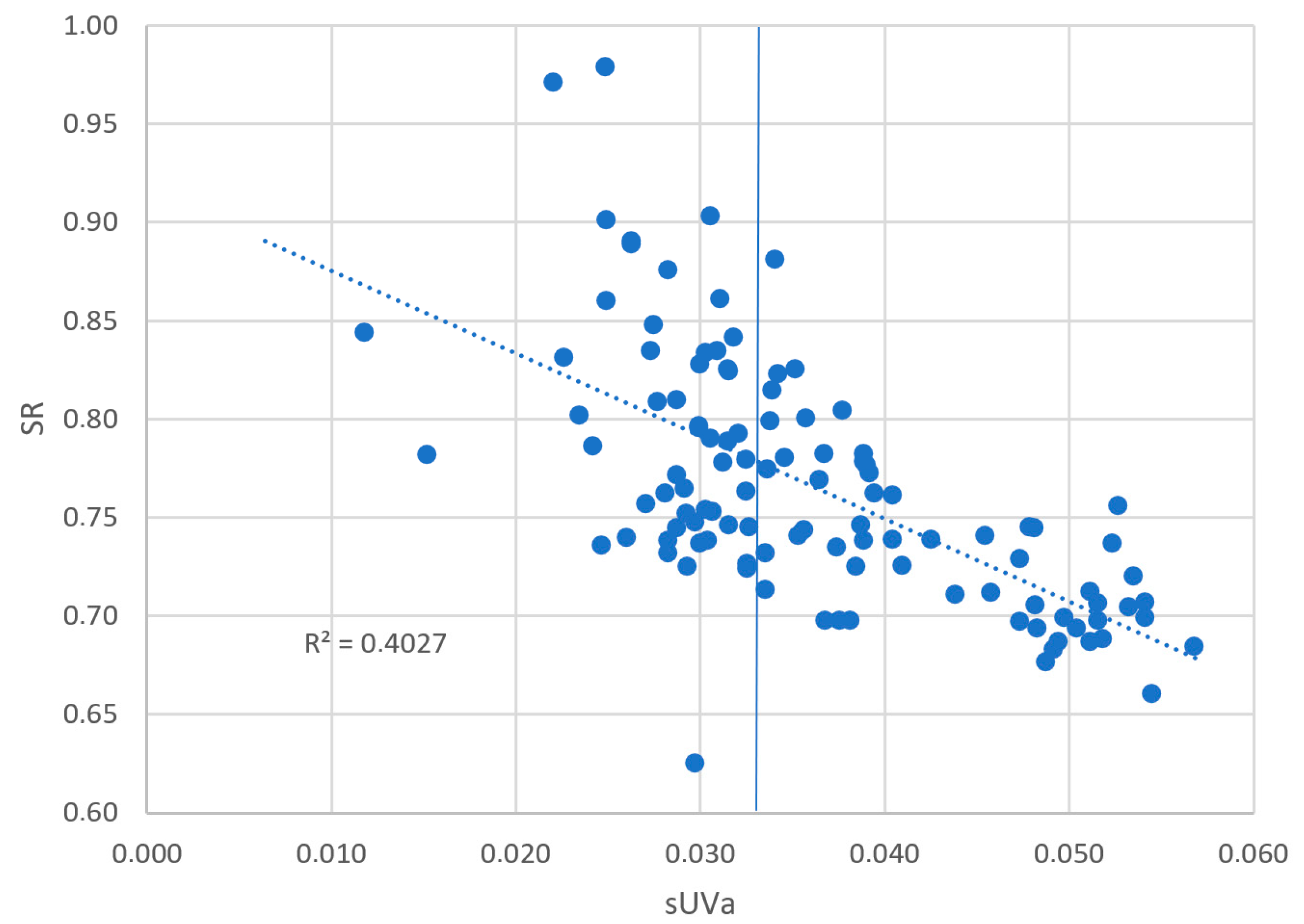
| VHA | sUVa | 0.669 |
| CHA | Urban | 0.689 |
| CODMn | 0.729 | |
| K+ | 0.676 | |
| NO3− | 0.729 | |
| BIX | 0.757 | |
| FI | 0.805 | |
| HIX | 0.704 |
Disclaimer/Publisher’s Note: The statements, opinions and data contained in all publications are solely those of the individual author(s) and contributor(s) and not of MDPI and/or the editor(s). MDPI and/or the editor(s) disclaim responsibility for any injury to people or property resulting from any ideas, methods, instructions or products referred to in the content. |
© 2023 by the authors. Licensee MDPI, Basel, Switzerland. This article is an open access article distributed under the terms and conditions of the Creative Commons Attribution (CC BY) license (https://creativecommons.org/licenses/by/4.0/).
Share and Cite
Vogt, R.D.; Porcal, P.; Hejzlar, J.; Paule-Mercado, M.C.; Haaland, S.; Gundersen, C.B.; Orderud, G.I.; Eikebrokk, B. Distinguishing between Sources of Natural Dissolved Organic Matter (DOM) Based on Its Characteristics. Water 2023, 15, 3006. https://doi.org/10.3390/w15163006
Vogt RD, Porcal P, Hejzlar J, Paule-Mercado MC, Haaland S, Gundersen CB, Orderud GI, Eikebrokk B. Distinguishing between Sources of Natural Dissolved Organic Matter (DOM) Based on Its Characteristics. Water. 2023; 15(16):3006. https://doi.org/10.3390/w15163006
Chicago/Turabian StyleVogt, Rolf David, Petr Porcal, Josef Hejzlar, Ma. Cristina Paule-Mercado, Ståle Haaland, Cathrine Brecke Gundersen, Geir Inge Orderud, and Bjørnar Eikebrokk. 2023. "Distinguishing between Sources of Natural Dissolved Organic Matter (DOM) Based on Its Characteristics" Water 15, no. 16: 3006. https://doi.org/10.3390/w15163006
APA StyleVogt, R. D., Porcal, P., Hejzlar, J., Paule-Mercado, M. C., Haaland, S., Gundersen, C. B., Orderud, G. I., & Eikebrokk, B. (2023). Distinguishing between Sources of Natural Dissolved Organic Matter (DOM) Based on Its Characteristics. Water, 15(16), 3006. https://doi.org/10.3390/w15163006