1. Introduction
Arid and semi-arid zones, characterized by limited rainfall compared to potential evapotranspiration, cover a significant portion of the Earth’s surface and are inhabited by approximately 35% of the global population, often with high levels of poverty [
1,
2]. Despite water scarcity, these regions are experiencing rapid population growth [
1,
3], leading to increased demands for water resources. Furthermore, climate variability and long-term trends exacerbate the existing challenges, placing additional stress on already scarce water supplies [
4,
5].
To effectively manage water resources in these areas, integrated strategies must be developed based on detailed knowledge of local hydrogeology conditions and other relevant factors. However, characterizing hydrogeology is challenging and costly, especially in remote or thinly settled agricultural regions [
6,
7]. The Coquimbo region in north-central Chile, the focus of this study, presents a case in point. This region has been severely impacted by climate variability, experiencing an extended period (~15 years) of low to very low precipitation, often referred to as a “mega-drought” [
8,
9,
10].
The rainfed, mid-mountain areas with moderate to steep slopes, situated between 200–2000 m above sea level (masl), have been particularly affected by this mega-drought. In these areas, the local population relies heavily on rainfall as the primary water source [
11].
Although these regions typically have low population density, recurrent water scarcity has imposed significant economic pressure on local governments responsible for ensuring water supply. For instance, between 2011 and 2014, the Coquimbo regional government spent over USD 10 million on water delivery, primarily through water trucks, to rural communities [
12]. The situation has further worsened, with expenditures exceeding USD 3.8 million in 2019 alone to address the effects of drought in the region. Paradoxically, these mid-mountain zones, which face recurring water scarcity, receive limited attention in hydrological and hydrogeological studies compared to the more economically productive floodplains and alluvial deposits of lower-lying river valleys and tributaries. Consequently, there is a lack of reliable information on water resources in these extensive, sparsely populated mid-mountain zones [
13,
14].
A previous study [
15] attempted to address this issue by using basic statistical and geostatistical techniques to assess the distribution of wells and springs in the dryland midmountain areas of the Coquimbo region. The authors identified linear patterns in the distribution, exhibiting two preferential orientations, NW and NE, which aligned with geological-structural controls rooted in the region’s Mesozoic and older structural features. However, the study acknowledged that incorporating new information, including both hard and soft data, could provide further insights into water availability. This includes the influence of natural attributes on local hydrological processes and the potential value of nontraditional inputs, such as anthropogenic features.
In this research, we aim to build upon the aforementioned study, by integrating information on natural factors (hydrological, lithological, structural, and geomorphological) and anthropogenic factors (social and road connectivity) simultaneously, which represents a novel aspect of our work. By utilizing GIS techniques and employing the Random Forest machine learning algorithm, we develop a groundwater potential map for the study area. Our objective is to assess how this approach can serve as a general framework for future groundwater resource development programs and aid in the early identification of vulnerable zones facing extended water shortage periods in rural areas, both within Chile and globally.
2. Area of Study
The study area is in the Coquimbo region, north-central Chile, between 29°02′ and 32°16′ S and 69°49′ and 71°40′ W. As previously mentioned, the area has experienced a severe drought period for almost 15 years.
Figure 1 illustrates the decline in annual rainfall amounts in Ovalle, located in the central part of the Region, from 1980 to 2020, highlighting the general trend of decreasing precipitation.
We focused on the middle mountain dryland zone between 200 and 2000 masl in elevation, corresponding to the N–S central belt of the region, which covers an area of approximately 23,200 km
2 (
Figure 2). The area transitions between semi-desert and mediterranean-desert climate [
16]; precipitation has an orographic dependence varying between 25 and 300 mm/year between the coastal areas and mountains, and there is a marked decrease in precipitation moving from south to north [
17]. Specifically for the dryland areas of the Coquimbo region that are of interest in the present work, precipitation registers mean values between 100 and 200 mm/year [
18,
19], with potential evapotranspiration greater than 1000 mm/year [
20].
The Coquimbo Region has a population of around 760,000, of which 81% live in urban and suburban areas near the coast, while the remaining 19% live in rural areas scattered mostly through the study area. A significant proportion of the rural population lives within a type of common property and land use system that dates from the nineteenth century, known as Comunidades Agrícolas (“Agricultural Communities”), which occurs almost exclusively in the Coquimbo Region. Due to the lack of permanent surface water courses, it is common for these communities to rely on water from springs or shallow wells, which, in turn, represents a constraint for a major, more intensive agricultural development [
20].
The study area is lacking in extensive sedimentary rock aquifers; in general, groundwater resources are present at shallow depths (tens to a few hundred meters) in areally-restricted deposits of volcanoclastic sediments, in granitic intrusives that have significant fracture permeability, or in weathering deposits of granitic origin (locally known as “maicillo”). The main source of recharge in the region is infiltration from winter precipitation in sporadic years of especially high rainfall, mainly associated with the El Niño phase of the ENSO phenomenon. Thus, given the isolated nature and limited storage in the aquifers, water supply in the region is extremely vulnerable to drought.
3. Methods
We conducted our analysis in four sequential steps: (1) Compilation of a database of known groundwater discharge locations (wells and springs); (2) Compilation of a spatial database of natural and anthropic factors potentially determining groundwater availability; (3) Analysis of the assembled data to develop a groundwater potential map; (4) Diagnostic checking of the map predictions and interpretation of the results (a general overview is given in
Figure 3). Each of these steps is discussed in more detail in the following sections.
3.1. Groundwater Discharge Database
We developed a database of groundwater discharge locations based on registered groundwater use rights available from the Chilean Water Authority (Dirección General de Aguas, DGA). Although the DGA data concentrate primarily on water wells, they also include information about springs. The DGA data were supplemented with a smaller set of wells supporting a photovoltaic irrigation program for small-scale farmers through the Instituto de Desarrollo Agropecuario (INDAP). Thus, we obtained information on a total of 5972 wells and 57 springs occurring within the study area.
From this dataset, we extracted all wells and springs located between 200 and 2000 masl. After a visual inspection of Google Earth images, we then removed any wells or springs located in irrigated agricultural land. This was done as their existence and location could potentially be influenced by irrigation water return-flows, i.e., excess infiltration from irrigated lands (that is recaptured in shallow wells or discharges from irrigation-sourced springs) and not by the different factors considered in this study. We also deleted any locations in alluvial fill where groundwater was most likely sourced from neighboring rivers or estuaries with permanent surface flow [
21]. The final database consisted of 3822 groundwater discharge points, comprising 3799 wells and 23 springs. For the sake of simplicity, we will not differentiate between wells and springs for the remainder of this paper, referring to both water sources as “wells”.
It is important to acknowledge that most wells in the database have low flow rates (
Table 1). Indeed, 87% of the wells have a declared discharge below 2 L/s, and less than 5% of the water sources in the database have flow rates greater than 10 L/s.
3.2. Groundwater Conditioning Factors (GCF)
Groundwater availability and flow are primarily determined by the interaction of multiple factors, such as climate, geomorphology (e.g., slope, drainage patterns), geology/lithology (e.g., rock type, presence, and characteristics of discontinuities in bedrock), and anthropogenic factors (e.g., land use). These can be referred to as “Groundwater Conditioning Factors” (GCFs). In the present study, we considered 21 GCFs that may influence the availability of groundwater, and therefore the spatial distribution of wells. The GCFs chosen for this work were selected based on literature review of studies in areas that were climatically and physiographically comparable to the Coquimbo region [
22,
23].
We also considered the actual availability in our study area of information on the various possible GCFs to be selected. We followed standard statistical protocol by binning continuous variables (e.g., elevation, slope, NDVI) into discrete categories to calculate meaningful probabilities and as an aid to graphical display of the results. Breaks between bins were chosen to correspond to natural divisions in the data, customary values in the literature, or as determined by expert judgment [
22]. Brief descriptions of the factors chosen, and the sources from which we obtained the values for each one, are presented as follows.
3.2.1. Topographic Factors
- -
Elevation: Probably the most considered topographic characteristic in groundwater potential studies is elevation (e.g., [
22,
24,
25]). Elevation is a natural constraint on human settlements, infrastructure, and road connectivity, and has been associated with the existence of springs [
26]. To obtain this layer, we downloaded twelve Digital Elevation Model (DEM) images (30 m resolution) of ASTER Global DEM (Terra satellite) from the USGS Earth Explorer web platform at
https://earthexplorer.usgs.gov/, accessed on 1 July, 2018. We processed the images using the Mosaicking and Clip Grid with Polygon modules of the System for Automated Geoscientific Analyses (SAGA/GIS, version 2.2.2) [
27]. To avoid the inherent complications in working with images of different granularity, we used the same 30 m resolution for all the topographic-related factors listed below.
- -
Slope: Slope may be an important factor for detecting areas of potential groundwater presence, since it has a dominant influence on the direction of surface water runoff and thus groundwater recharge [
28]. We derived information on slope from the raster elevation data using the Slope function in ArcGIS (version 10.3).
- -
Aspect: The aspect, or direction towards which sloping ground faces, was determined based on the maximum downward slope (i.e., steepest descent) from the center of an area to the surrounding areas. To evaluate this, Arc Map’s Aspect function was applied to the elevation data. The result is an azimuth for each pixel from 0° (north) clockwise to 360°, represented by an orientation code in 45° increments.
- -
Terrain Ruggedness Index (TRI): TRI characterizes the topographic heterogeneity of the terrain. We used the Terrain Ruggedness Index module of SAGA/GIS to extract a non-dimensional measure of TRI.
- -
Topographic Wetness Index (TWI): Previous investigations have proposed that elevated soil moisture at a given site indicates an area retains more water than it loses; thus, such locations are favorable for recharge and may indicate higher groundwater potential [
29]. We used the Topographic Wetness Index (One Step) module of SAGA/GIS to estimate the TWI [
30].
- -
Distance to Drainage Network: A textural analysis of the drainage network assists in the evaluation of the characteristics of groundwater recharge zones [
31]. The SAGA/GIS module Channel Network was applied to the elevation raster data to develop this layer. We chose an “initiation threshold” of 1 × 10
7 and a “minimum segment length” of 50 m [
19]. The resulting vector layer, in polyline shapefile format, included a total of 1122 lines within the study area, most of which exhibited a dendritic drainage pattern. From this, we obtained the distance from the nearest drainage network line, in meters, to each pixel, by applying the Euclidean Distance function of Arc Map to the vector output of the Drainage Network command.
- -
Drainage Network Density: We used the Line Density function of Arc Map, with a search radius of 1000 m, to extract this layer from the shapefile vector output of the Drainage Network module (see above). The output of this operation is a pixel (raster) value indicating the total length of the drainage network per pixel surface area (units of km/km2, or 1/km).
The following six factors are all slightly different measures of the same characteristic of topography (that is, curvature of the topographic surface). Although redundancy between these factors may limit their usefulness, there are small differences in their ability to discriminate between behaviors. Ultimately, however, subsequent analyses showed that none of these six factors appeared in the top ranks as indicators of groundwater availability. In
Section 3 (i.e., Results and Discussion), we therefore limit our discussion to the influence of the first-listed of these factors (Convergence Index), while the remaining five factors are described here primarily for the sake of completeness.
- -
Convergence Index (CI): The relief structure of a terrain can be classified as belonging to either convergent areas (“channels”) or divergent areas (“ridges”). The CI was estimated from elevation and orientation data using the SAGA/GIS Convergence Index module.
- -
General Curvature: This parameter identifies deviations from a hypothetical horizontal plane as being either convex or concave areas within the terrain. It was obtained using the Curvature function in Arc Map. Positive values indicate a convex-upward surface, while negative values indicate concave-upward surfaces and a flat surface has a value of zero [
32].
- -
Plan Curvature: It is related to the convergence or divergence of flow at a given surface location (a pixel), measured perpendicular to the direction of the maximum slope [
33]. We generated this layer using the Curvature function of Arc Map.
- -
Profile Curvature: The profile curvature refers to the curvature of a line formed by the intersection of an imaginary vertical plane and the ground surface along the line of steepest descent [
34]. As with the general curvature (above), we calculated profile curvature by applying the Curvature function of ArcGIS.
- -
Convexity: The convexity of each pixel was evaluated applying the Terrain Surface Convexity module of SAGA/GIS.
- -
Concavity: This relief attribute gives the opposite result to the Convexity layer, identifying flat or concave-upward areas (valleys or gullies), where sediments and runoff tends to naturally accumulate. It was obtained with the Terrain Surface Convexity module of SAGA/GIS.
3.2.2. Geological Factors
- -
Lithology: Rock types often play an important role in determining the occurrence and distribution of groundwater [
35]. We evaluated the distribution of lithology in our study area using the 1:1,000,000 scale geological map of Chile [
36], simplified according to the suggestions of [
15]. We also changed the resulting vector format to raster data using the Arc Map functions Polygon to Raster and Reclassify, to obtain a layer with a spatial resolution of 30 m, in keeping with the resolution of the topographic factors listed in the previous section.
- -
Distance to Faults: First, we obtained fault locations from [
36] and supplemented these with fault maps for the study area by [
37]. The two sources of data were joined using the Merge module in Arc Map. From this, the distance to fault layer was generated by applying the Euclidean Distance function in Arc Map to the data of the Fault layer. The resulting raster data consists of the distance, in meters, between a given pixel and the nearest mapped fault, at 30 m resolution.
- -
Fault Density: We used the Line Density function in Arc Map with a search radius of 1000 m to generate a 30 m resolution raster layer of fault density, expressed in units of linear length of fault traces per area (km/km2 or, equivalently, 1/km).
3.2.3. Vegetation-Related Factors
We used the vegetation indices NDVI and SAVI to characterize vegetation cover in the study area. For both layers, we used six scenes downloaded from the USGS web platform (earthexplorer.usgs.gov, accessed on 1 July 2018), dated 11 January 2000, and 18 January 2000. These dates are during summer in the field area, in an active La Niña year. We chose this timing for the images under the assumption that the soil cover would be representative of stable, non-seasonal vegetation indicative of perennial soil water and, ultimately, elevated recharge. In addition, we made atmospheric and topographic corrections to the spectral bands of the satellite images (i.e., the six scenes) in SAGA/GIS, using the procedure described by [
38].
- -
NDVI: This index uses the contrast of the absorption of the red bank of the electromagnetic spectrum by chlorophyll pigment and the high reflectivity of plant materials in the near-infrared bank to generate an estimate of “greenness,” or relative vegetation biomass [
39]. We used the Vegetation Index (Slope Based) module of SAGA/GIS, applied to input data from Band 4 (“B4”, 0.77–0.90 μm) and Band 3 (“B3”, 0.63–0.69 μm) from Landsat 7 ETM+ images; from this information, we calculated NDVI from [
40]:
The result was a 30 m resolution raster layer, with values −1 ≤ NDVI ≤ +1.
- -
SAVI: Like NDVI, SAVI is a measure of vegetation reflectance, but SAVI incorporates an adjustment factor, L, that accounts for the brightness of the ground surface underlying the vegetation. We used a value of L = 0.5, which was suggested by [
41] as appropriate for arid zones. A SAVI raster layer at the required 30 m resolution was obtained by applying the Vegetation Index (Slope Based) module of SAGA/GIS to Band 4 and Band 3 of the Landsat 7 ETM+ images.
3.2.4. Anthropic Factors
- -
Agricultural communities: As explained earlier, the Comunidades Agrícolas (Agricultural Communities) are an ancient, spatially extended form of land tenure in rural North-Central Chile, especially in the Coquimbo Region, in which partially hereditary groups organize common ownership and occupy, exploit, or cultivate rural land for forestry and/or farming [
42]. This practice dates back at least to Spanish colonial times (i.e., the 17th century) and continues today. Because of the heavy dependence of agricultural activity on groundwater resources in rural dryland areas, it is reasonable to expect a strong association between wells locations and agricultural communities. It is unclear, however, whether the current locations of human settlements are the result of ease of access to groundwater, or if the need for water resources to support agriculture drives exploration and exploitation of groundwater, and both may be true.
Despite the fact that what was described corresponds to a “chicken vs. egg” type of situation where it is not easy to distinguish causality, it was nevertheless considered of interest in this work to incorporate agricultural communities as one of the GCFs assessed. Thus, data on the existence and distribution of agricultural communities [
18,
43] were processed as a raster layer (30 m resolution) using the Polygon to Raster and Reclassify functions of Arc Map. The resulting Agricultural Communities layer consisted of binary (i.e., 0 or 1) pixel values in which 1 indicates that the pixel belongs to the territory of a community and 0 indicates that the pixel is not part of the holdings of an agricultural community.
- -
Distance to roads: In a study in Iraq, it was shown that wells were preferentially located in proximity to existing facilities or infrastructure such as roads [
44]. With this in mind, we decided to incorporate this element as an additional GCF, based on the shapefile Red Caminera de Chile (“Chilean road network”) available at
www.mapas.mop.cl, accessed 1 August 2018. From the road network layer, we generated the distance to roads layer using the Euclidean Distance function of Arc Map. The result was a raster layer at 30 m resolution of pixel values indicating distance in meters from each pixel to the nearest road.
- -
Road Density: We used the Line Density function of Arc Map with a search radius of 500 m to obtain a raster layer at 30 m resolution, with pixel values indicating the length of roads per square kilometer of surface area for that pixel (units of km/km2, or, equivalently, 1/km).
3.3. Frequency Ratios
Although not being the core technique in this work (which is presented in the next subsection), frequency ratio (FR) was initially calculated as a preliminary method to identify and illustrate, in a simple way, the quantitative relationship between the presence of wells and the classes of the different GCFs [
24]. The FR is defined as [
22,
24]:
where A is the area occupied by a given bin of the factor, B is the total area occupied by the factor, C is the number of pixels occupied by the factor, and D is the total number of pixels in the domain. Equation (2) is equivalent to the ratio between the “percentage of area with wells for each class of a factor divided by the percentage of the domain for each class of a factor” [
29], and previous investigators interpret values of FR > 1 as an indication of strong association between wells and a (sub)class of a factor, whereas values FR < 1 generally indicate a lower or weaker association [
22]. In this study, we extended the concept of the FR to apply not only to the presence of wells, but also to the percentage of discharge associated with the subclasses of each GCF (i.e., the percentage of discharge for each class of a factor divided by the percentage of the domain for each class of a factor).
3.4. Groundwater Potential Model
3.4.1. The Random Forest Algorithm and the Groundwater Potential Map
In this study, we used the Random Forest (RF) algorithm to predict the presence of wells (and, by extension, inferred groundwater availability) within our study area, considering this problem as a binary classification task where the predicted probability of presence is returned. The RF model, which belongs to the family of “Machine Learning” techniques, was first introduced by [
45]. Machine Learning (ML) is defined as a subfield of computer science that gives computers the ability to learn without being explicitly programmed; of existing ML techniques, RF is considered one of the most powerful of the fully automated ML algorithms [
46]. Two good reviews of the RF method have been published relatively recently [
47,
48], the second one being specifically oriented to the applications of RF in assessments of water resources.
For the present study, we chose to use the Random Forest (RF) algorithm as implemented in ModelMap package [
49] of the statistical computing environment R as the solely ML algorithm as this technique has shown its superior performance across several families of ML models including neural networks and deep neural networks. ModelMap builds predictive models of continuous or categorical response variables using an RF algorithm, giving the user the option to validate the models with independent test data sets or out-of-bag (OOB) estimates on the training data. The package comprises three main R packages: PresenceAbsence, randomForest and raster; together, these packages allow user-friendly modeling, validation, and mapping of response variables over large geographic areas within the R computational framework [
50,
51]. The versions used were: R, version 4.0.5; ModelMap, version 3.4.0.3; and raster, version 3.5-15.
To train the RF algorithm for the study area, we complemented the database of 3822 wells with an additional set of 3820 randomly located points corresponding to absence of wells (it was verified that they actually were displayed in areas with no wells); thus, the algorithm classified each pixel according to the presence/absence of wells and associated these categories with the GCFs. The presence/absence database was divided into training (70%) and validation (30%) subsets [
24]. The model output (for each 30 × 30 m pixel) were probability values (of predicting the presence of a well) ranging from 0 to 1 [
23]. The model was initially built with 1000 trees (ntree = 1000), as it is not possible to know a priori when the stabilization of the error will occur [
52]. In any case, a sensitivity analysis on this hyperparameter, as well as on mtry (number of variables to try at each node of RF trees), is given in
Appendix A.
From this, we obtained a groundwater potential map using the modelmap make function of the ModelMap package, considering four categories: low, moderate, high, and very high groundwater potential (corresponding to output probabilities from 0 to 0.24, from 0.25 to 0.49, from 0.5 to 0.74, and above 0.74, respectively).
3.4.2. Model Assessment
We used two main approaches to assess two separate aspects of the RF model: performance and interpretation in terms of variable importance. For model performance we selected Receiver Operating Characteristics (ROC), the Area under the Curve (AUC), sensitivity, specificity and Kappa. For model interpretation we used Variable Importance based on Mean Decrease Accuracy (MDA), and Mean Decrease Gini (MDG). These measures of model performance and interpretation are described in more detail below.
- -
Classification performance: The Receiver Operating Characteristics (ROC) curve is a method for quantifying model prediction accuracy in binary classification problems that is commonly applied to probabilistic models and forecasting systems [
26,
50,
51]; in particular, this method has been used to assess model accuracy in groundwater potential mapping studies (e.g., [
46,
53,
54]). The ROC curve is a cumulative probability plot of “true positive rates” (also known as sensitivity), versus “false positive rates” (also known as specificity) for a range of cutoff values (thresholds for detection). At the same time, we calculated the associated Area Under the Curve (AUC), a threshold independent measure of model quality. In this context AUC is a number between 0 and 1; the closer a value is to 1, the better the ability of the model to discriminate between the cases, with 1 indicating perfect discrimination. An AUC of 0.5 indicates the model predictions are the same as a random guess, while values between 0 and 0.5 imply the model is worse at prediction than a random guess [
24,
51].
- -
Variable importance: The relative importance of the GCFs was evaluated using two measures: the Mean Decrease Accuracy (MDA) and the Mean Decrease Gini (MDG) [
46,
55]. MDA measures the difference in model accuracy before and after a permutation of the predictor variable values. A low value of MDA indicates that the response (predicted) variable is relatively insensitive to changes (permutations) of the predictor variable. Conversely, a predictor variable is considered “important” when there is a significant difference between the value of the response variable before and after the change (i.e., a higher value of MDA is obtained). On the other hand, MDG measures the ability of a predictor variable to correctly separate and group cases within a dataset that tend to fall into the same class during construction of an RF model [
47]. In the present work, this implies separating and accurately grouping cases where wells exist, in comparison to cases where wells are absent. The larger the magnitude of MDG for a given variable, the better classifier it is. According to [
46], MDA is more important for variable selection, while MDG is more important for defining explanatory associations between selected variables.
4. Results and Discussion
4.1. Relationships between GCFs, Wells and Discharge by FR
The relationships of various GCFs and their subclasses to the presence of wells and related discharge are presented in
Table 2 and
Figure 4. The former includes areas, number of wells, and nominal discharge (i.e., cumulative total for all the wells for each subclass of the GCFs), along with the FR values for both wells (FR
W) and discharge (FR
Q).
It is clear from inspection of the entries in
Table 2 that FR
W and FR
Q are closely correlated, so, except for special cases as noted below, the following remarks are valid for either metric.
With respect to topographically related GCFs, the analyses presented in
Table 2 indicate that wells, and the corresponding discharges, are preferentially associated to areas of low elevation (most predominantly in the range of 200–500 masl), low slope (less than 5°), and low ruggedness (TRI < 4). This is consistent with the findings of previous investigators (e.g., [
22,
24,
29]), who generally agree that higher elevations, steeper slopes, and greater surface curvatures are associated with higher runoff, lower infiltration, and therefore reduced potential for groundwater occurrence.
It is worthwhile examining the FR values obtained for the Convergence Index (CI). The highest values are associated with the “high divergence” subclass, an outcome that tends to be counterintuitive. In fact, this result is obtained because of the small percent area (0.2% of the total study area), which distorts the calculation by placing a small number in the denominator of the ratio. In fact, careful inspection of the values in
Table 2 shows that by far most wells and discharge are associated with flat to low-divergence surfaces in the range of −25 ≤ CI ≤ 5, with counts n
c = 3086, whereas highly divergent surfaces (−100 ≤ CI ≤ −50) only accounted for n
c = 60 counts. The appearance of this artifact highlights a generally not addressed weakness of using FR as an indicator of the importance of a conditioning variable and requires careful interpretation of the results of this type of qualitative measure.
With respect to non-topographic GCFs, there is a notable association of groundwater (wells and discharge) with areas of moderate to dense vegetation, as would be expected for locations where the water table is located near the surface. In terms of surficial geology, groundwater occurrences are primarily associated with Neogene sediments, and secondarily in association with granitic rocks. In this case, the differences between FRW and FRQ are likely significant, since the highest discharges are associated with wells in the Neogene sediments, which possess higher primary hydraulic conductivities. Associations with other geological factors, such as distance to faults or fault densities, are not observed. Unsurprisingly, however, the highest FR values occur for higher drainage densities and shorter distances from the drainage network, and anthropic factors such as the presence of agricultural communities and the distance to, and density of, roads are factors of apparent importance.
4.2. RF Model Performance Analysis
As discussed before, from the original 7642-point dataset, we trained the RF classification algorithm based on a 70/30 ratio of train–test split and estimated model performance in terms of OOB prediction on the training data and the independent test set.
Table 3 presents the AUC, sensitivity, specificity and Kappa performance metric. The overall performance can be considered high for classification tasks as AUC approaches 1 and Kappa can be considered substantial or good, the same as for sensitivity and specificity.
Figure 5 shows the behavior of the classification errors by type and OOB error as the number of decision trees in the RF model increases. All types of errors can be seen to decrease rapidly until around 200 decision trees, after which the rate of improvement in the models decreases and the number of errors stabilizes. At around 600 decision trees the so called “convergence of errors” is reached, after which the prediction quality does not improve, regardless of how much the number of trees is increased.
The general characteristics of the model are presented graphically in
Figure 6 and
Figure 7.
Figure 6A shows histograms of the number of predictions of the presence and absence of wells for the full range of probability cutoffs for the presence of wells. This figure shows that the vast majority of true detects (presence) have prediction probabilities above 0.4, while the majority of true non-detects (absence) fall below prediction probabilities of 0.6. Given the double humped distribution presented here, we chose a probability of 0.5 for the presence/absence cutoff value. In
Figure 6B, the prediction probability is seen to increase as the number of observations within the bin increases, approximately along the 1:1 line, which indicates a “well-calibrated” model [
50].
Figure 7A presents the ROC-AUC curve, also known as the “success rate,” from the training stage. The area under the ROC-AUC curve represents the probability that a point chosen as a presence (a well detect) has a higher predicted probability than a point that is not a well. For the present study, the model has an approximately 95% probability of making a correct classification. Alternative measures of model accuracy are presented in
Figure 6B; specifically, sensitivity, specificity, and “Kappa,” where the cutoff probability is plotted on the abscissa and the magnitude of the accuracy measurements are plotted on the ordinate.
These measures of accuracy tend to converge when the model is well calibrated and has good discrimination capacity [
50]. In the present case, sensitivity and specificity converge near 0.87, while the maximum value of Kappa is close to 0.74. It has been suggested that such values represent a “moderate to near-strong fit” [
46], and [
23] obtained Kappa values of 0.42, 0.61, and 0.43 for Random Forest, MARS, and C5.0 models, respectively. Integrating the performance metrics considered above provides support for a value of 0.5 as a reasonable cutoff probability separating the presence and absence of groundwater.
4.3. RF Model Interpretation in Terms of Relative Importance of GCFs
4.3.1. GCFs of High Importance
In
Figure 8, we present graphically two rankings (MDA and MDG) of the importance of the GCFs considered for the development of the RF model, which can be used for interpreting the effects of individual model predictors.
The higher the ranking received by a variable, the more important it is as an indicator of groundwater presence. Anthropic factors (agricultural communities and road distance) feature prominently in the top three factors of both measures (MDA and MDG), consistent with a strong human influence on the location of wells. This is obviously the case for agricultural communities, where wells are a key element for subsistence-farming activities associated with these communities. Similarly, the distance to roads is likely to be an important indication of well location, because it is associated with the use, access, construction, and maintenance of wells. Therefore, it turns out that in our study area, the existence (or non-existence) of wells is not solely a function of natural (geologic, topographic, etc.) factors, but is strongly dependent on anthropogenic factors as well. Similar findings were reported in [
56], where it was shown that man-made water sources (wells and qanats) tend to be preferentially placed in areas with lower slope angles, and generally at lower elevations, that are commonly associated with agriculture. This is different from the findings of investigators working on the development of spring potential maps (i.e., natural groundwater outflow), who found much less dependence on anthropogenic features, and much greater dependence on topographical and hydrogeological characteristics [
22,
57,
58].
It is worthwhile to perform an additional analysis with respect to this result. In this respect, it could be thought that the distance to roads could indeed determine the convenience of drilling a well, but that by itself would not necessarily be an indicator of favorable conditions for the presence of groundwater. However, it is important to remember the physiographic characteristics of the study area of the present work, i.e., areas of mountainous relief. In this context, it is to be expected that the roads are built and arranged through the valleys (low areas) between the slopes of the hills. In fact,
Figure 9 presents a given longitudinal profile in the middle part of the study area. As can be seen in the figure, the (rural) roads correspond, as well as the gulches (dry creeks), to low areas, which would be consistent to a water sink, i.e., an area with an accumulation of water (associated with the runoff that flows from the surrounding slopes of the hills). Thus, the fact that roads have evidenced a special importance as GCF is not entirely random but can be associated, quite reliably, with a physically based situation.
For non-anthropic (i.e., natural) GCFs, the influence of elevation stands out in the MDA rankings. Based on the MDG ranking, both slope and ruggedness index show a high level of importance. As discussed previously, these factors are directly related to runoff and infiltration processes, and therefore to the availability of groundwater.
4.3.2. GCFs of Low Importance
In addition to identifying GCFs of high importance for locating groundwater resources, it is worthwhile to examine some of the variables that have been used as indicators of groundwater potential in previous studies, but which did not demonstrate a high importance ranking in the current one. In particular, the factors Lithology and Fault Density placed at or near the bottom of both the MDA and MDG rankings, although previous investigations have found good associations with these factors [
15].
In terms of lithology, the Neogene sediments are generally high in permeability, although their areal extent is relatively small (only 12.6% of the study area). The low area occupied by these sediments likely accentuates the calculated values of FR (
Table 2), similar to the FR values for CI, and the high discharges associated with wells in these sediments clearly influence the discharge-based values (FRQ = 4.8, versus FRW = 2.0). However, the small percentage of the study area occupied by these sediments may render them relatively unimportant for classification in the RF model. In addition, the maps upon which the distribution of lithology were based may not be sufficiently detailed (i.e., large-scaled) to adequately represent the distribution of the high permeability, but areally restricted Neogene sediments. Granitic rocks, on the other hand, commonly demonstrate only modest permeability, primarily arising from near-surface fracturing; locally, however, areas of maicillo deposits (weathered sediments) may have high permeability (and therefore high discharge). Because the high permeability areas are restricted in areal extent, granitic rocks as a category likely do not present to the RF model a consistent association with either wells or discharge.
For the GCF Fault Density, the two sources of fault data used in this study [
36,
37] are mapped at a scale consistent with the present analysis; however, they specifically identify the surface traces of faults, and they concentrate on mapping major features. In contrast, most wells are likely associated with secondary fracturing, and are rarely located in the plane of a major fault. A detailed examination of wells and mapped faults in the Punitaqui sub-basin located in the middle part of the study area [
6] and presenting a high density of wells (
Figure 2), shows apparent groupings of them in clusters, many of which appear to be aligned along NW and NE linear trends (
Figure 10). However, there is little, if any, visual association with the mapped faults in the area. Although it is possible that the wells align along faults that are too small to have been included in the maps used in this study, without more detailed fault mapping it must be concluded that fault density turned out to be, at best of minor importance, for the regional (i.e., 100 s km) study scale approach considered in this work.
Previous investigators have obtained results that are rather similar to those of the present study for the influence of both lithology and faulting on groundwater potential. Using an RF model [
24], lithology was found to be the tenth and thirteenth out of thirteen factors (10/13 and 13/13) ranked by MDA and MDG, respectively, in their study of springs at the Moghan Basin, Iran. The investigators found mixed results for the influence of faulting on groundwater potential, with distance to faults ranking moderately high in importance (3/13 and 5/13 for MDA and MDG, respectively), but fault density only being of secondary importance (6/13 and 10/13 for MDA and MDG, respectively). Furthermore, neither fault density nor distance to faults were ranked as having any importance by other ML methods (Classification and Regression Tree/CART or Boosted Regression Tree/BRT) they used. Other more recent studies have, in general, obtained results that have also shown that fault density is not an important indicator of groundwater potential, whereas the results for distance from faults varies from moderate importance to insignificant (e.g., [
7,
23,
55,
59]. In summary, although geological-structural elements such as faulting have an intuitive appeal as important controls on groundwater occurrence [
15], since the presence and/or density of faults influence recharge processes [
59] and groundwater migration patterns, ML based studies find they are of moderate or low utility as indicators of groundwater.
4.4. Groundwater Potential Map
The key output of the RF model is the groundwater potential map for the study area, presented in
Figure 11.
Most of the study area is classified as low groundwater potential (GWP). Only about 14.1% of the total study area is classified as high or very high GWP; the majority of the high or very high GWP areas are restricted to narrow zones near riverbeds or alluvial fill deposits, with some additional zones in the west-central and southwest portions of the study area. Also, a qualitative inspection of the validation wells for a sub-area plotted in
Figure 11B shows that existing wells do, indeed, lie within the zones of high and very high GWP.
It is worth noting that the well database upon which the RF model was based consisted primarily of wells with low flow rates, and this characteristic of the data must be considered when interpreting the results presented in a map such as
Figure 11. Thus, areas of high or very high GWP do not necessarily equate to high flow rates. In a practical sense, however, this is not an important restriction on the significance and usefulness of the map. Because the region is lightly populated and groundwater use is dominated by individual landholders and small agricultural communities, there is little need for high-yield wells. Thus, for this region, the groundwater potential map of
Figure 11 therefore constitutes an appropriate guide for future groundwater exploration efforts.
Additionally, the model output may be important for assessing areas at greater risk of water shortage. Indeed, the study area is in a region of the country that is subject to recurring water scarcity [
8,
12], and these problems are likely to continue or worsen in response to changing climate. Thus, it is reasonable to expect that wells located in regions of low or moderate GWP may be more vulnerable to a decrease in precipitation and/or excessive exploitation than wells located in higher GWP areas. A useful and interesting extension of the present study might be to refine the assessment of “at risk” areas using the groundwater potential map, with other indications of groundwater stress (e.g., data on well abandonment), as inputs to an ML evaluation specifically addressing water resource vulnerability.
4.5. Final Remarks
Together with the above-mentioned considerations, it is useful to assess the reliability of the GWP map in terms of the characteristics of existent wells as a function of GWP classes in the validation set. For that, we formed a characterization matrix for the pixels with wells (presence) in the test set. The characterization matrix (
Table 4) shows the number of wells (both counts and as a percentage of the total number of wells in the test set) that fall into pixels with a given GWP. In addition, we provide the total discharge in L/s and as a percentage of the total discharge for all wells in the validation dataset for the wells in each GWP class, and the areal coverage represented by the pixels in each category.
According to
Table 4, approximately 86% of the validation wells were in areas of high to very high groundwater potential, which provides confidence in the predictive quality of the model. As was discussed previously, there is no requirement for the wells located in the high or very high GWP areas to have high discharge rates individually (i.e., per well); however, these two categories account for 77% of the total granted discharge of the validation wells dataset.
Taken together, the main findings discussed in this section support the conclusion that the developed model is a reliable indicator of zones with high potential for groundwater. Keeping in mind the caveat, discussed before, that high groundwater potential does not necessarily equate to high discharge rates in the study area, the probability map obtained and the methodology used in its construction have at least two practical applications in the context of water resource management in the arid to semi-arid areas of Chile and elsewhere: (a) they provide valuable information on groundwater potential to guide exploration for future groundwater resources; and (b) they are likely to be useful for identifying rural areas most vulnerable to changing climate and extended drought, such as that which the region has been experiencing for the past >10 years.
5. Conclusions
Arid and semi-arid regions, covering over 30% of the Earth’s land surface, face challenges due to limited water resources and the impacts of climate change. To mitigate the effects of drought and changing precipitation patterns, it is crucial to develop water resource management strategies based on a deep understanding of the local hydrologic cycle. However, detailed characterization of hydrogeology in rural or remote areas is often economically unfeasible.
In this study, we present a case study of the Coquimbo region in north-central Chile, a thinly settled arid to semi-arid area where traditional field investigations for hydrogeology characterization are impractical. Instead, we employed Geographic Information System (GIS) and machine learning (ML) tools to analyze natural and anthropogenic factors, aiming to evaluate groundwater potential. By utilizing the Random Forest (RF) ML technique and originally considering 21 groundwater conditioning factors (GCFs) along with existing springs and wells data, we developed a regional-scale groundwater potential map. The RF approach demonstrated reliable identification of areas with high groundwater potential, achieving significant performance levels with an AUC of 0.95 and Kappa of 0.74 for the study area.
Surprisingly, our study revealed that natural factors such as bedrock geology and faulting were relatively weak indicators of groundwater potential, contrary to initial expectations.
Lithology and fault density ranked low among the 21 GCFs, aligning with findings from other ML-based studies. Conversely, anthropogenic factors emerged as strong indicators of groundwater presence, occupying top positions in terms of important criteria (Mean Decrease Accuracy, or MDA, and Mean Decrease Gini, or MDG) investigated in this study.
Practically, the application of ML techniques allowed us to discern patterns of wells and leverage past groundwater exploration and exploitation experiences. This approach enables the identification of areas with high groundwater potential, even if they currently lack wells, making them suitable for future exploration efforts. It is important to note that although an area may exhibit high groundwater potential, it does not necessarily guarantee high discharge rates. While this limitation is not significant for this study, as the wells primarily serve individuals or small agricultural communities with relatively low yield requirements, incorporating discharge considerations would be necessary when applying the methodology to explore high-yield wells for municipal or industrial purposes.
Moreover, besides its relevance in groundwater exploration, the groundwater potential map developed in this study holds valuable insights into areas sensitive to drought, overuse, and water stress. The Coquimbo region, like many arid and semi-arid regions worldwide, has been grappling with water scarcity for over a decade. Wells located in low groundwater-potential areas are particularly vulnerable to the impacts of changing climate, precipitation patterns, and infiltration rates. Identification of these vulnerable zones using the groundwater potential map can serve as an initial step for targeted governmental intervention, aimed at alleviating the long-term water scarcity challenges faced by affected rural communities.
Finally, and based on the findings of this study, some recommendations can be made for future research and water resource management in arid and semi-arid regions: (1) Integration of anthropogenic factors: The significant influence of anthropogenic factors on groundwater potential suggests the importance of considering human activities and infrastructure in water resource management strategies. Incorporating data on social factors, road connectivity, and other anthropogenic features can enhance the accuracy and effectiveness of groundwater potential mapping; (2) Validation and refinement: While the Random Forest (RF) approach showed promising results in this study, further validation and refinement of the model should be pursued; (3) Continued collection of groundwater data, including well yield and discharge rates, can help improve the accuracy of groundwater potential predictions and ensure their applicability to different contexts; (4) Long-term monitoring: Given the impacts of climate change and the prolonged water scarcity experienced in arid and semi-arid regions, long-term monitoring of groundwater resources is crucial. Regular monitoring can provide valuable insights into the dynamics of groundwater availability, recharge rates, and potential impacts of climate variability. This information can guide adaptive management strategies and facilitate early detection of water stress.
Author Contributions
Conceptualization, J.M.D., J.N., J.P.F., J.L.A. and R.O.; methodology, J.M.D., J.N. and R.O.; software, J.M.D. and J.N.; validation, J.M.D. and J.N.; formal analysis, J.M.D., J.N., J.P.F. and R.O.; writing—original draft preparation, J.M.D., J.N., J.P.F., R.O. and J.L.A.; writing—review and editing, J.N., J.P.F., R.O. and J.L.A.; project ad- ministration, R.O.; funding acquisition, R.O., J.N. and J.L.A. All authors have read and agreed to the published version of the manuscript.
Funding
This research was supported by ANID/FONDECYT/1150587 and ANID/FONDAP/15130015. At the same time, Jorge Núñez Cobo acknowledges the financial support of DIDULS/ULS, through the project N° PAAI21195.
Data Availability Statement
This work has been developed upon public databases as described in the manuscript.
Acknowledgments
We acknowledge the participation of Jorge Oyarzún who was a main contributor of this work from conception to completion. We thank Nataly Diaz for her help in developing
Figure 7. Jorge Núñez acknowledges the financial support of DIDULS/ULS, through the project PAAI21195, and José Luis Arumí and Ricardo Oyarzún acknowledge the financial support of ANID/FONDAP/15130015. The paper greatly benefited from the comments of two reviewers for which we thank.
Conflicts of Interest
The authors declare no conflict of interest.
Appendix A
Two hyperparameters of the Random Forest models were chosen for sensitivity analysis: The number of random forest trees of the RF model (ntree) and the number of variables to try at each node of RF trees (mtry). The set of selected values for each hyperparameter can be compared with default values used during model building (ntree = 1000, mtry = p/3 where p is the number of predictors, 21 in our case). Note that for reproducibility, a seed = 40 was used to avoid randomness in the outcomes and to account only for the selected hyperparameters in the results obtained.
Table A1.
Sensitivity analysis of Random Forest (RF) performance metrics with respect to the number of random forest trees of the RF model (ntree) and the number of variables to try at each node of RF trees (mtry).
Table A1.
Sensitivity analysis of Random Forest (RF) performance metrics with respect to the number of random forest trees of the RF model (ntree) and the number of variables to try at each node of RF trees (mtry).
| ntree | 250 | 500 | 1000 |
|---|
| mtry | 3 | 7 | 10 | 15 | 3 | 7 | 10 | 15 | 3 | 7 | 10 | 15 |
|---|
| AUC | 0.944 | 0.942 | 0.942 | 0.941 | 0.944 | 0.943 | 0.942 | 0.941 | 0.945 | 0.943 | 0.943 | 0.942 |
| Sensitivity | 0.895 | 0.897 | 0.901 | 0.897 | 0.893 | 0.900 | 0.898 | 0.900 | 0.896 | 0.898 | 0.897 | 0.899 |
| Specificity | 0.855 | 0.855 | 0.859 | 0.857 | 0.855 | 0.856 | 0.857 | 0.860 | 0.854 | 0.857 | 0.856 | 0.856 |
| Kappa | 0.750 | 0.753 | 0.760 | 0.754 | 0.748 | 0.756 | 0.755 | 0.760 | 0.750 | 0.755 | 0.754 | 0.755 |
References
- Scanlon, B.R.; Keese, K.E.; Flint, A.L.; Flint, L.E.; Gaye, C.B.; Edmunds, M.; Simmers, I. Global synthesis of groundwater recharge in semiarid and arid regions. Hydrol. Process. 2006, 20, 3335–3370. [Google Scholar]
- Lictevout, E. Acces a l’eau des Populations Vulnerables en Zone Aride: Un Probleme de Ressource, de Gestion ou d’information? Thèse pour Obtenir le Grade de Docteur de l’Université de Montpellier. 2018. Available online: https://theses.hal.science/tel-02045888/document (accessed on 5 November 2022).
- UNDDD. United Decade for Desert and the Fight against Desertification. 2017. Available online: http://www.un.org/en/events/desertification_decade/whynow.shtml (accessed on 12 August 2019).
- Arab Water Council. Vulnerability of Arid and Semi-Arid Regions to Climate Change: Impacts and Adaptive Strategies. Online Report. 2009. Available online: https://www.eldis.org/document/A60488 (accessed on 21 August 2021).
- Souvignet, M.; Gaese, H.; Ribbe, L.; Kretschmer, N.; Oyarzún, R. Statistical downscaling of precipitation and temperature in North-Central Chile: An assessment of possible climate change impacts in an arid Andean watershed. Hydrol. Sci. J. 2010, 55, 41–57. [Google Scholar] [CrossRef]
- Sandoval, E.; Baldo, G.; Núñez, J.; Oyarzún, J.; Fairley, J.P.; Ajami, H.; Arumí, J.L.; Aguirre, E.; Maturana, H.; Oyarzún, R. Groundwater recharge assessment in a rural, arid, mid-mountain basin in North-Central Chile. Hydrol. Sci. J. 2018, 63, 1873–1889. [Google Scholar] [CrossRef]
- Razavi-Termeh, S.V.; Khosravi, K.; Sadeghi-Niaraki, A.; Choi, S.; Singh, V.P. Improving groundwater potential mapping using metaheuristic approaches. Hydrol. Sci. J. 2020, 65, 2729–2749. [Google Scholar] [CrossRef]
- Núñez, J.; Rivera, D.; Oyarzún, R.; Arumí, J.L. Influence of Pacific Ocean multidecadal variability on the distributional properties of hydrological variables in north-central Chile. J. Hydrol. 2013, 501, 227–240. [Google Scholar] [CrossRef]
- Garreaud, R.D.; Alvarez-Garreton, C.; Barichivich, J.; Boisier, J.P.; Christie, D.; Galleguillos, M.; LeQuesne, C.; McPhee, J.; Zambrano-Bigiarini, M. The 2010–2015 megadrought in central Chile: Impacts on regional hydroclimate and vegetation. HESS 2017, 21, 6307–6363. [Google Scholar] [CrossRef]
- Garreaud, R.D.; Boisier, J.P.; Rondanelli, R.; Montecinos, A.; Sepúlveda, H.H.; Veloso-Aguila, D. The Central Chile Mega Drought (2010–2018): A climate dynamics perspective. Int. J. Climatol. 2020, 40, 421–439. [Google Scholar] [CrossRef]
- CNID. Ciencia e Innovación para los Desafíos del agua en Chile. Consejo Nacional de Innovación para el Desarrollo. 2016. Available online: https://ctci.minciencia.gob.cl/wp-content/uploads/2017/07/Ciencia-e-Innovaci%C3%B3n-para-los-Desaf%C3%ADos-del-Agua-en-Chile-2017.pdf (accessed on 21 March 2020).
- CR2. Report to the Nation. The 2010–2015 Mega-Drought: A Lesson for the Future. Center for Climate and Resilience Research. 2015. Available online: http://www.cr2.cl/wp-content/uploads/2015/11/Megadrought_report.pdf (accessed on 18 September 2019).
- Taucare, M.; Daniele, L.; Viguier, B.; Vallejos, A.; Arancibia, G. Groundwater resources and recharge processes in the Western Andean Front of Central Chile. Sci. Total Environ. 2020, 722, 137824. [Google Scholar] [CrossRef]
- Taucare, M.; Viguier, B.; Daniele, L.; Heuser, G.; Arancibia, G.; Leonardi, V. Connectivity of fractures and groundwater flows analyses into the Western Andean Front by means of a topological approach (Aconcagua Basin, Central Chile). Hydrogeol. J. 2020, 28, 2429–2438. [Google Scholar] [CrossRef]
- Oyarzún, R.; Oyarzún, J.; Fairley, J.; Núñez, J.; Gómez, N.; Arumí, J.; Maturana, H. A simple approach for the analysis of the structural-geologic control of groundwater in an arid rural, mid-mountain, granitic and volcanic-sedimentary terrain: The case of the Coquimbo Region, North-Central Chile. J. Arid Environ. 2017, 142, 31–35. [Google Scholar] [CrossRef]
- Novoa, J.; López, D. IV Región: El escenario Geográfico Físico. In Libro Rojo de la Flora Nativa y de los Sitios Prioritarios para su Conservación: Región de Coquimbo, Capítulo 2; Squeo, F., Arancio, G., Gutiérrez, J., Eds.; Ediciones Universidad de La Serena: La Serena, Chile, 2001; pp. 13–28. Available online: http://www.biouls.cl/lrojo/Manuscrito/Capitulo%2002%20Escenario%20Geografico.PDF (accessed on 1 March 2019).
- Favier, V.; Falvey, M.; Rabatel, A.; Praderio, E.; López, D. Interpreting discrepancies between discharge and precipitation in high-altitude area of Chile’s Norte Chico region (26–32°S). Water Resour. Res. 2009, 45, W02424. [Google Scholar] [CrossRef]
- CNR. Estudio de los Recursos Hídricos en el Secano de IV Región para una Propuesta de Desarrollo Agrícola. Comisión Nacional de Riego. 2003. Available online: https://bibliotecadigital.ciren.cl/handle/20.500.13082/9499 (accessed on 1 August 2021).
- Tapia, S. Identificación y Evaluación de Zonas Potenciales de Recarga de Aguas Subterráneas en el Sector de la Mina Escuela Brillador Mediante Sistemas de Información Geográfica. BSc graduation work, Civil and Environmental Engineering. University of La Serena, La Serena, Chile, 2015. [Google Scholar]
- Luengo, P.; Oyarzún, R.; Oyarzún, J.; Alvarez, P.; Canut de Bon, C. Aguas subterráneas en macizos rocosas fracturados: Su utilización en zonas rurales montañosas del Centro Norte de Chile. In Proceedings of the VIII Congreso Latino Americano de Hidrología Subterránea (ALSHUD), Asunción, Paraguay, 25–29 September 2006. [Google Scholar]
- Gómez, N. Relaciones Geohidrológicas en Cuencas de la Región de Coquimbo, con Énfasis en Zonas de Secano de Media Montaña. BSc graduation work, Civil and Environmental Engineering. University of La Serena, La Serena, Chile, 2017; p. 896. [Google Scholar]
- Naghibi, S.A.; Pourghasemi, H.R.; Pourtaghi, Z.S.; Rezaei, A. Groundwater qanat potential mapping using frequency ratio and Shannon´s entropy models in the Moghan watershed, Iran. Earth Sci. Inform. 2015, 8, 171–186. [Google Scholar] [CrossRef]
- Golkarian, A.; Naghibi, S.A.; Kalantar, B.; Pradhan, B. Groundwater potential mapping using C5.0, random forest, and multi- variate adaptive regression spline models in GIS. Environ. Monit. Assess. 2018, 190, 149. [Google Scholar] [CrossRef]
- Naghibi, S.A.; Pourghasemi, H.R.; Dixon, B. GIS-based groundwater potential mapping using boosted regression tree, classifi-cation and regression tree, and random forest machine learning models in Iran. Environ. Monit. Assess. 2016, 188, 44. [Google Scholar] [CrossRef] [PubMed]
- Taheri, F.; Jafari, H.; Rezaei, N.; Bagheri, R. The use of continuous fuzzy and traditional classification models for groundwater potentially mapping in areas underlain by granitic hard-rock aquifers. Environ. Earth Sci. 2020, 79, 91. [Google Scholar] [CrossRef]
- Mousavi, S.; Golkarian, A.; Naghibi, S.; Kalantar, B.; Pradhan, B. GIS-based Groundwater spring potential mapping Using Data Mining Boosted Regression Tree and Probabilistic Frequency Ratio Model in Iran. AIMS Geosci. 2017, 3, 91–115. [Google Scholar]
- Conrad, O.; Bechtel, B.; Bock, M.; Dietrich, H.; Fischer, E.; Gerlitz, L.; Wehberg, J.; Wichmann, V.; Böhner, J. System for Automated Geoscientific Analyses (SAGA) v. 2.1.4. GMD 2015, 8, 1991–2007. [Google Scholar] [CrossRef]
- Prasanta, G.; Sujay, B.; Narayan, C. Mapping of groundwater potential zones in hard rock terrain using geoinformatics: A case of Kumari watershed in western part of West Bengal. MESE 2016, 2, 1. [Google Scholar] [CrossRef]
- Oh, H.; Kim, Y.; Choi, J.; Park, E.; Lee, S. GIS mapping of regional probabilistic groundwater potential in the area of Pohang City, Korea. J. Hydrol. 2011, 399, 158–172. [Google Scholar] [CrossRef]
- Kopecký, M.; Čížková, Š. Using topographic wetness index in vegetation ecology: Does the algorithm matter? Appl. Veg. Sci. 2010, 13, 450–459. [Google Scholar] [CrossRef]
- Tessema, A.; Mengistu, H.; Chirenje, E.; Abiye, T.; Demlie, M. The relationship between lineaments and borehole yield in North West Province, South Africa: Results from geophysical studies. Hydrogeol. J. 2012, 20, 351–368. [Google Scholar] [CrossRef]
- ESRI. Qué es Arc Map. ArcGIS for Desktop. Available online: http://desktop.arcgis.com/es/arcmap/10.3/main/map/what-is-arcmap-.htm (accessed on 1 March 2018).
- ESRI. Curvatura. ArcGIS for Desktop. Available online: https://desktop.arcgis.com/es/arcmap/10.3/tools/spatial-analyst-toolbox/curvature.htm (accessed on 1 March 2018).
- Ohlmacher, G. Plan curvature and landslide probability in regions dominated by earth flows and earth slides. Eng. Geol. 2007, 91, 117–134. [Google Scholar] [CrossRef]
- Yeh, H.F.; Cheng, Y.S.; Lin, H.I.; Lee, C.H. Mapping groundwater recharge potential zone using a GIS approach in Hualian River, Taiwan. Sustain. Environ. Res. 2016, 26, 33–43. [Google Scholar] [CrossRef]
- SERNAGEOMIN. Mapa Geológico de Chile (1:1.000.000). Servicio Nacional de Geología y Minería. Available online: http://www.ipgp.fr/~dechabal/Geol-millon.pdf (accessed on 4 July 2018).
- Tidy, E. Estudio Geológico-Estructural basado en Imágenes Landsat de Chile entre los paralelos 18oS y 35oS. In Geología y Recursos Minerales de Chile; Frutos, J., Oyarzun, R., Pincheira, M., Eds.; Editorial Universidad de Concepción: Concepción, Chile, 1986; Volume 1, pp. 136–202. [Google Scholar]
- Oyarzún, J.; Núñez, J.; Fairley, J.P.; Tapia, S.; Alvarez, D.; Maturana, H.; Arumí, J.L.; Aguirre, E.; Carvajal, A.; Oyarzún, R. Groundwater Recharge Assessment in an Arid, Coastal, Middle Mountain Copper Mining District, Coquimbo Region, North-central Chile. Mine Water Environ. 2019, 38, 226–242. [Google Scholar] [CrossRef]
- ESRI. Función NDVI. ArcGIS for Desktop. Available online: https://pro.arcgis.com/es/pro-app/latest/help/analysis/raster-functions/ndvi-function.htm (accessed on 28 June 2023).
- USGS. Landsat Surface Reflectance-Derived Spectral Indices. 2021. Available online: https://www.usgs.gov/core-science-systems/nli/landsat/landsat-normalized-difference-vegetation-index (accessed on 3 March 2020).
- Squeo, F.; Tracol, Y.; López, D.; Gutiérrez, J.; Cordova, A.; Ehleringer, J. ENSO effects on primary productivity in southern Atacama Desert. ADGEO 2006, 6, 273–277. [Google Scholar] [CrossRef]
- Wilkins, J.; Greene, F. Comunidades Agrícolas: Antecedentes Generales y Jurídicos. Biblioteca del Congreso Nacional, Valparaíso. Available online: https://www.bcn.cl/obtienearchivo?id=repositorio/10221/19924/1/COMUNIDADES%20AGRICOLAS.f_v4.doc (accessed on 2 January 2019).
- Livenais, P.; Aranda, X. Dinámica de los Sistemas Agrarios en Chile Árido: La Región de Coquimbo; LOM: Santiago, Chile, 2003. [Google Scholar]
- Al-Abadi, A. Groundwater potential mapping at northeastern Wasit and Missan Governorates, Iraq using a data-driven weights of evidence technique in framework of GIS. Environ. Earth Sci. 2015, 74, 11091124. [Google Scholar] [CrossRef]
- Breiman, L. Random Forest. Mach. Learn. 2001, 45, 5–32. [Google Scholar] [CrossRef]
- Al-Abadi, A.; Shahid, S. Spatial mapping of artesian zone at Iraqi southern desert using a GIS-based random forest machine learning model. MESE 2016, 2, 96. [Google Scholar] [CrossRef]
- Biau, G.; Scornet, E. Rejoinder on: A random forest guided tour. TEST 2016, 25, 264–268. [Google Scholar] [CrossRef]
- Tyralis, H.; Papacharalampous, G.; Langousis, A. A Brief Review of Random Forests for Water Scientists and Practitioners and Their Recent History in Water Resources. Water 2019, 11, 910. [Google Scholar] [CrossRef]
- Freeman, E.; Frescino, T.; Moisen, G. ModelMap: An R Package for Model Creation and Map Production. 2016. Available online: https://cran.r-project.org/web/packages/ModelMap/vignettes/VModelMap.pdf (accessed on 9 March 2019).
- Freeman, E.A.; Moisen, G. PresenceAbsence: An R Package for Presence-Absence Model Analysis. J. Stat. Softw. 2008, 23, 1–31. Available online: http://www.jstatsoft.org/v23/i11 (accessed on 1 September 2018). [CrossRef]
- Rahmati, O.; Pourghasemi, H.; Melesse, A. Application of GIS-based data driven random forest and maximum entropy models for groundwater potential mapping: A case study at Mehran Region, Iran. Catena 2016, 137, 360–372. [Google Scholar] [CrossRef]
- Gao, X.; Wang, K.; Lo, K.; Wen, R.; Huang, X.; Dang, Q. Water poverty assessment based on the random forest algorithm: Application to Gansu, Northwest China. Water Policy 2021, 23, 1388–1399. [Google Scholar] [CrossRef]
- Balamurugan, G.; Seshan, K.; Bera, S. Frequency ratio model for groundwater potential mapping and its sustainable management in cold desert, India. J. King Saud Univ. Sci. 2017, 29, 333–347. [Google Scholar]
- Sameen, M.I.; Pradhan, B.; Lee, S. Self-Learning Random Forests Model for Mapping Groundwater Yield in Data-Scarce Areas. Nat. Resour. Res. 2018, 28, 757–775. [Google Scholar] [CrossRef]
- Zabihi, M.; Pourghasemi, H.; Pourtaghi, Z.; Behzadfar, M. GIS-based multivariate adaptive regression spline and random forest models for groundwater mapping in Iran. Environ. Earth Sci. 2016, 75, 665. [Google Scholar] [CrossRef]
- Naghibi, S.; Moghaddam, D.; Kalantar, B.; Pradhan, B. A comparative assessment of GIS-based data mining models and a novel ensemble in groundwater well potential mapping. J. Hydrol. 2017, 548, 471–483. [Google Scholar] [CrossRef]
- Ozdemir, A. Using binary logistic regression method and GIS for evaluating and mapping the groundwater spring potential in the Sultan Mountains (Aksehir, Turkey). J. Hydrol. 2011, 405, 123–136. [Google Scholar] [CrossRef]
- Ozdemir, A. GIS-based groundwater spring potential mapping in the Sultan Mountains (Konya, Turkey) using frequency ratio, weights of evidence and logistic regression methods and their comparison. J. Hydrol. 2011, 411, 290–308. [Google Scholar] [CrossRef]
- Doke, A.; Pardeshi, S.; Das, S. Drainage morphometry and groundwater potential mapping: Application of geoinformatics with frequency ratio and influencing factor approaches. Environ. Earth Sci. 2020, 79, 393. [Google Scholar] [CrossRef]
Figure 1.
Annual rainfall amounts for the city of Ovalle (Ovalle-DGA station, 30°36′15″ S, 71°12′30″ W) for the period 1980–2020.
Figure 1.
Annual rainfall amounts for the city of Ovalle (Ovalle-DGA station, 30°36′15″ S, 71°12′30″ W) for the period 1980–2020.
Figure 2.
Coquimbo Region, specific area considered in the study (elevations between 200 and 2000 masl) and distribution of groundwater discharge locations (wells and springs).
Figure 2.
Coquimbo Region, specific area considered in the study (elevations between 200 and 2000 masl) and distribution of groundwater discharge locations (wells and springs).
Figure 3.
Methodological flowchart.
Figure 3.
Methodological flowchart.
Figure 4.
Groundwater Conditioning Factors (GCFs) and subclasses considered in this work (for the sake of clarity and information, the figure also include the thematic layers of drainage network, faults, and roads, that are not GCFs by themselves, but are required to obtain some of them).
Figure 4.
Groundwater Conditioning Factors (GCFs) and subclasses considered in this work (for the sake of clarity and information, the figure also include the thematic layers of drainage network, faults, and roads, that are not GCFs by themselves, but are required to obtain some of them).
Figure 5.
RF model classification error (the green line corresponds to class 1 error or presence, the red line corresponds to class 0 error, and the black line corresponds to OOB error).
Figure 5.
RF model classification error (the green line corresponds to class 1 error or presence, the red line corresponds to class 0 error, and the black line corresponds to OOB error).
Figure 6.
Prediction histogram (A) and calibration plot (B). In (A) the black color within each bar corresponds to the cases that are wells (presences) while the gray color for those cases corresponds to non-well cases (absences).
Figure 6.
Prediction histogram (A) and calibration plot (B). In (A) the black color within each bar corresponds to the cases that are wells (presences) while the gray color for those cases corresponds to non-well cases (absences).
Figure 7.
Success rate (A) and performance metrics (B) of the RF model. The diagonal grey line (A) represents the ROC curve for random guessing.
Figure 7.
Success rate (A) and performance metrics (B) of the RF model. The diagonal grey line (A) represents the ROC curve for random guessing.
Figure 8.
Mean decrease accuracy (A) and mean decrease Gini (B) of the RF model.
Figure 8.
Mean decrease accuracy (A) and mean decrease Gini (B) of the RF model.
Figure 9.
Google Earth-based elevation profile (at 636 masl; 30°57′ S, 71°11′ W). Orange lines show the presence of roads, whereas blue ones correspond to gulches (dry creeks). Blue arrows represent potential infiltrated water movement from higher to lower zones.
Figure 9.
Google Earth-based elevation profile (at 636 masl; 30°57′ S, 71°11′ W). Orange lines show the presence of roads, whereas blue ones correspond to gulches (dry creeks). Blue arrows represent potential infiltrated water movement from higher to lower zones.
Figure 10.
Distribution of wells and lineaments in the Punitaqui basin (for its location look at
Figure 1).
Figure 10.
Distribution of wells and lineaments in the Punitaqui basin (for its location look at
Figure 1).
Figure 11.
Groundwater potential map (A) and detailed view of selected zone (B).
Figure 11.
Groundwater potential map (A) and detailed view of selected zone (B).
Table 1.
Distribution of wells by flow range.
Table 1.
Distribution of wells by flow range.
| Discharge (L/s) | Frequency | % |
|---|
| 0.01–1 | 2928 | 76.61 |
| 1.1–2 | 430 | 11.25 |
| 2.1–5 | 298 | 7.80 |
| 5.1–10 | 64 | 1.68 |
| 10.1–50 | 90 | 2.35 |
| 50.1–100 | 10 | 0.26 |
| >100 | 2 | 0.05 |
Table 2.
GCF (classes and subclasses) characterization and wells and discharge distributions. nT: Total number of wells; nc: Number of wells for each subcategory; QT: Total discharge (granted); Qs: Cumulative discharge of wells for each subcategory; AT: Total Area; Ac: Area for each subcategory; FRW: Frequency ratio of wells; FRQ: Frequency ratio of discharge.
| | nT: 3822 | QT: 5154.5 L/s | AT: 23,235.2 km2 | FRW | FRQ |
|---|
| GCF | nc | (%) | QS (L/s) | (%) | Ac (km2) | (%) | | |
| Topographic Factors | | | | | | | | |
| Elevation (masl) | | | | | | | | |
| 200–500 | 1814 | 47.4 | 3135.4 | 60.8 | 5146 | 22.1 | 2.1 | 2.8 |
| 500–1000 | 1704 | 44.6 | 1656.0 | 32.1 | 8592 | 37.0 | 1.2 | 0.9 |
| 1000–1500 | 262 | 6.9 | 346.0 | 6.7 | 5961 | 25.7 | 0.3 | 0.3 |
| 1500–2000 | 42 | 1.1 | 17.1 | 0.3 | 3537 | 15.2 | 0.1 | 0.0 |
| Slope (°) | | | | | | | | |
| 0–5 | 1689 | 44.2 | 2738.2 | 53.1 | 2538 | 10.9 | 4.1 | 4.9 |
| 5–10 | 1370 | 35.9 | 1640.6 | 31.8 | 3980 | 17.1 | 2.1 | 1.9 |
| 10–15 | 444 | 11.6 | 437.2 | 8.5 | 4041 | 17.4 | 0.7 | 0.5 |
| 15–30 | 303 | 7.9 | 303.5 | 5.9 | 10,059 | 43.3 | 0.2 | 0.1 |
| 30–45 | 16 | 0.4 | 34.9 | 0.7 | 2592 | 11.2 | 0.0 | 0.1 |
| 45–72 | 0 | 0.00 | 0.00 | 0.00 | 25 | 0.1 | 0.0 | 0.0 |
| Aspect (°) | | | | | | | | |
| | Flat terrain | 0 | 0 | 0 | 0 | 26 | 0.1 | 0.0 | 0.0 |
| 337.5–22.5 | N | 767 | 20.1 | 927.0 | 18.0 | 2875 | 12.4 | 1.6 | 1.5 |
| 22.5–67.5 | NE | 519 | 13.6 | 608.4 | 11.8 | 2736 | 11.8 | 1.2 | 1.0 |
| 67.5–112.5 | E | 399 | 10.4 | 323.2 | 6.3 | 2567 | 11.0 | 0.9 | 0.6 |
| 112.5–157.5 | SE | 289 | 7.6 | 436.3 | 8.5 | 2472 | 10.6 | 0.7 | 0.8 |
| 157.5–202.5 | S | 257 | 6.7 | 412.7 | 8.0 | 2574 | 11.1 | 0.6 | 0.7 |
| 202.5–247.5 | SW | 389 | 10.2 | 699.4 | 13.6 | 3283 | 14.1 | 0.7 | 1.0 |
| 247.5–292.5 | W | 504 | 13.2 | 966.4 | 18.7 | 3470 | 14.9 | 0.9 | 1.3 |
| 292.5–337.5 | NW | 698 | 18.2 | 781.0 | 15.1 | 3233 | 13.9 | 1.3 | 1.1 |
| Terrain Ruggedness Index, TRI (m) | | | | | | | | |
| 0–4 | Flat terrain surface | 3032 | 79.3 | 4376.6 | 84.9 | 6534 | 28.1 | 2.8 | 3.0 |
| 4–8 | Near flat surface | 671 | 17.6 | 536.2 | 10.4 | 8065 | 34.7 | 0.5 | 0.3 |
| 8–12 | Moderately rugged surface | 100 | 2.6 | 206.4 | 4.0 | 5589 | 24.1 | 0.1 | 0.2 |
| 12–16 | Highly rugged surface | 16 | 0.4 | 25.8 | 0.5 | 2474 | 10.6 | 0.0 | 0.0 |
| 16–70 | Extremely rugged surface | 3 | 0.1 | 9.3 | 0.2 | 574 | 2.5 | 0.0 | 0.1 |
| Topographic Wetness Index, TWI | | | | | | | | |
| 2.6–6.6 | Very low | 674 | 17.63 | 1147.1 | 22.2 | 13,859 | 59.6 | 0.3 | 0.4 |
| 6.6–9 | Low | 1287 | 33.68 | 1436.99 | 27.9 | 6333 | 27.3 | 1.2 | 1.0 |
| 9–12.2 | Moderate | 945 | 24.73 | 1139.65 | 22.1 | 2179 | 9.4 | 2.6 | 2.4 |
| 12.2–16.7 | High | 694 | 18.15 | 1128.91 | 21.9 | 684 | 2.9 | 6.3 | 7.6 |
| 16.7–26.6 | Very high | 222 | 5.81 | 301.84 | 5.9 | 180 | 0.7 | 8.3 | 8.4 |
| Distance to Drainage Network (m) | | | | | | | | |
| 0–500 | 1682 | 44.01 | 3471.78 | 67.35 | 4974 | 21.4 | 2.1 | 3.1 |
| 500–1000 | 639 | 16.72 | 729.41 | 14.15 | 4321 | 18.6 | 0.9 | 0.8 |
| 1000–2000 | 928 | 24.28 | 706.18 | 13.70 | 6985 | 30.1 | 0.8 | 0.5 |
| >2000 | 573 | 14.99 | 247.11 | 4.79 | 6951 | 29.9 | 0.5 | 0.2 |
| Drainage Network Density (km/km2) | | | | | | | | |
| 0–0.1 | 1626 | 42.54 | 1034.18 | 20.06 | 14,534 | 62.6 | 0.7 | 0.3 |
| 0.1–0.5 | 491 | 12.85 | 552.51 | 10.72 | 2751 | 11.8 | 1.1 | 0.9 |
| 0.5–1 | 1413 | 36.97 | 2702.67 | 52.43 | 4919 | 21.2 | 1.7 | 2.5 |
| 1–2 | 292 | 7.64 | 865.12 | 16.78 | 1015 | 4.4 | 1.7 | 3.8 |
| 2–5.32 | 0 | 0 | 0 | 0 | 12 | 0.1 | 0.0 | 0.0 |
| Convergence Index | | | | | | | | |
| (−100)–(−50) | Highly divergent surface | 60 | 1.57 | 116.42 | 2.26 | 40 | 0.2 | 7.9 | 11.3 |
| (−50)–(−25) | Moderate divergent surface | 338 | 8.84 | 409.62 | 7.95 | 355 | 1.5 | 5.9 | 5.3 |
| (−25)–(−5) | Low divergent surface | 1452 | 37.99 | 1365.21 | 26.49 | 3941 | 17.0 | 2.2 | 1.6 |
| (−5)–5 | Flat surface | 1634 | 42.75 | 2602.18 | 50.48 | 14,525 | 62.5 | 0.7 | 0.8 |
| 5–25 | Low convergent surface | 318 | 8.32 | 625.48 | 12.13 | 4048 | 17.4 | 0.5 | 0.7 |
| 25–50 | Moderate convergent surface | 18 | 0.47 | 35.07 | 0.68 | 273 | 1.2 | 0.4 | 0.6 |
| 50–100 | Highly convergent surface | 2 | 0.05 | 0.50 | 0.01 | 54 | 0.2 | 0.3 | 0.1 |
| General Curvature (1/100 m) | | | | | | | | |
| (−10)–(−0.72) | High concavity | 268 | 7.01 | 242.08 | 4.70 | 1812 | 7.8 | 0.9 | 0.6 |
| (−0.72)–(−0.28) | Medium concavity | 1101 | 28.81 | 1226.70 | 23.80 | 4698 | 20.2 | 1.4 | 1.2 |
| (−0.28)–(0.15) | Flat surface | 1903 | 49.79 | 2555.54 | 49.58 | 8328 | 35.8 | 1.4 | 1.4 |
| 0.15–0.66 | Medium convexity | 519 | 13.58 | 1037.91 | 20.14 | 6123 | 26.4 | 0.5 | 0.8 |
| 0.66–7.9 | High convexity | 31 | 0.81 | 92.24 | 1.79 | 2275 | 9.8 | 0.1 | 0.2 |
| Plain Curvature (1/100 m) | | | | | | | | |
| (−4.46)–(−0.4687) | High concavity | 180 | 4.71 | 86.28 | 1.67 | 1466 | 6.3 | 0.7 | 0.3 |
| (−0.4687)–(−0.161) | Medium concavity | 915 | 23.94 | 1042.40 | 20.22 | 4498 | 19.4 | 1.2 | 1.0 |
| (−0.161)–0.0841 | Flat surface | 1920 | 50.24 | 2556.58 | 49.60 | 8275 | 35.6 | 1.4 | 1.4 |
| 0.0841–0.3913 | Medium convexity | 763 | 19.96 | 1370.23 | 26.58 | 6577 | 28.3 | 0.7 | 0.9 |
| 0.391–3.37 | High convexity | 44 | 1.15 | 98.99 | 1.92 | 2419 | 10.4 | 0.1 | 0.2 |
| Profile Curvature (1/100 m) | | | | | | | | |
| (−7.49)–(−0.57) | High convexity | 7 | 0.18 | 82.67 | 1.60 | 794 | 3.4 | 0.1 | 0.5 |
| (−0.57)–(−0.21) | Medium convexity | 181 | 4.74 | 183.55 | 3.56 | 3652 | 15.7 | 0.3 | 0.2 |
| (−0.21)–0.022 | Flat surface | 1189 | 31.11 | 1837.73 | 35.65 | 7258 | 31.2 | 1.0 | 1.1 |
| 0.022–0.377 | Medium concavity | 2037 | 53.30 | 2617.27 | 50.78 | 9222 | 39.7 | 1.3 | 1.3 |
| 0.377–7.60 | High concavity | 408 | 10.68 | 433.25 | 8.41 | 2309 | 9.9 | 1.1 | 0.8 |
| Convexity | | | | | | | | |
| 0–20 | Flat surface | 0 | 0.00 | 0.00 | 0.00 | 31 | 0.1 | 0.0 | 0.0 |
| 20–40 | Very low convexity | 602 | 15.75 | 822.51 | 15.96 | 2123 | 9.1 | 1.7 | 1.8 |
| 40–45 | Low convexity | 1425 | 37.28 | 1617.69 | 31.38 | 4661 | 20.1 | 1.9 | 1.6 |
| 45–50 | Medium convexity | 1485 | 38.85 | 2362.07 | 45.83 | 6851 | 29.5 | 1.3 | 1.6 |
| 50–60 | High convexity | 309 | 8.08 | 351.96 | 6.83 | 8210 | 35.3 | 0.2 | 0.2 |
| 60–83.3 | Very high convexity | 1 | 0.03 | 0.25 | 0.00 | 1359 | 5.8 | 0.0 | 0.0 |
| Concavity | | | | | | | | |
| 0–20 | Flat surface | 0 | 0.00 | 0.00 | 0.00 | 16 | 0.1 | 0.0 | 0.0 |
| 20–40 | Very low concavity | 1 | 0.03 | 0.25 | 0.00 | 1370 | 5.9 | 0.0 | 0.0 |
| 40–45 | Low concavity | 32 | 0.84 | 30.06 | 0.58 | 2871 | 12.4 | 0.1 | 0.0 |
| 45–50 | Medium concavity | 278 | 7.27 | 323.90 | 6.28 | 5352 | 23.0 | 0.3 | 0.3 |
| 50–60 | High concavity | 2909 | 76.11 | 3977.76 | 77.17 | 11,520 | 49.6 | 1.5 | 1.6 |
| 60–84.5 | Very high concavity | 602 | 15.75 | 822.51 | 15.96 | 2106 | 9.1 | 1.7 | 1.8 |
| Geological Factors | | | | | | | | |
| Lithology | | | | | | | | |
| Cenozoic to Paleozoic granitic rocks | 2130 | 55.73 | 1246.33 | 24.18 | 9716 | 41.8 | 1.3 | 0.6 |
| Neogen sediments | 985 | 25.77 | 3114.74 | 60.43 | 2918 | 12.6 | 2.0 | 4.8 |
| Mesozoic to Cenozoic volcanic-sedimentary rocks | 707 | 18.50 | 793.41 | 15.39 | 10,601 | 45.6 | 0.4 | 0.3 |
| Distance to Faults (m) | | | | | | | | |
| 0–500 | 791 | 20.70 | 1215.99 | 23.59 | 5282 | 22.7 | 0.9 | 1.0 |
| 500–1000 | 714 | 18.68 | 980.28 | 19.02 | 4256 | 18.3 | 1.0 | 1.0 |
| 1000–2000 | 1024 | 26.79 | 1064.15 | 20.65 | 5982 | 25.7 | 1.0 | 0.8 |
| >2000 | 1293 | 33.83 | 1894.06 | 36.75 | 7715 | 33.2 | 1.0 | 1.1 |
| Fault Density (km/km2) | | | | | | | | |
| 0–0.1 | 2378 | 62.22 | 3010.29 | 58.4 | 14,077 | 60.6 | 1.0 | 1.0 |
| 0.1–0.5 | 545 | 14.26 | 900.85 | 17.48 | 3176 | 13.7 | 1.0 | 1.3 |
| 0.5–1 | 777 | 20.33 | 1139.71 | 22.11 | 4887 | 21.0 | 1.0 | 1.1 |
| 1–2 | 121 | 3.17 | 103.42 | 2.01 | 1082 | 4.7 | 0.7 | 0.4 |
| 2–2.8 | 1 | 0.03 | 0.20 | 0.00 | 13 | 0.1 | 0.3 | 0.0 |
| Vegetation-Related Factors | | | | | | | | |
| NDVI | | | | | | | | |
| (−1)–0 | Water body | 0 | 0.00 | 0.00 | 0 | 48 | 0.2 | 0.0 | 0.0 |
| 0–0.1 | Non-vegetated soil | 344 | 9.00 | 1563.50 | 30.33 | 7381 | 31.8 | 0.3 | 1.0 |
| 0.1–0.25 | Prairies and shrubs | 2364 | 61.85 | 2090.45 | 40.56 | 13,126 | 56.5 | 1.1 | 0.7 |
| 0.25–1 | Dense covered vegetation (growth peak) | 1114 | 29.15 | 1500.53 | 29.11 | 2679 | 11.5 | 2.5 | 2.5 |
| SAVI | | | | | | | | |
| (−1.5)–0 | Water body | 0 | 0.00 | 0.00 | 0.00 | 48 | 0.2 | 0.0 | 0.0 |
| 0–0.1 | Non-vegetated soil | 71 | 1.86 | 700.77 | 13.60 | 2325 | 10.0 | 0.2 | 1.4 |
| 0.1–0.5 | Prairies and shrubs | 3226 | 84.41 | 3574.50 | 69.35 | 19,729 | 84.9 | 1.0 | 0.8 |
| 0.5–1 | Medium cover density vegetation | 520 | 13.61 | 871.14 | 16.90 | 1059 | 4.6 | 3.0 | 3.7 |
| 1–1.5 | Dense covered vegetation, forest | 5 | 0.13 | 8.07 | 0.16 | 74 | 0.3 | 0.4 | 0.5 |
| Anthropic Factors | | | | | | | | |
| Agricultural Communities | | | | | | | | |
| Present | 2754 | 72.06 | 1559.40 | 30.25 | 7584 | 32.6 | 2.2 | 0.9 |
| Absents | 1068 | 27.94 | 3595.07 | 69.75 | 15,651 | 67.4 | 0.4 | 1.0 |
| Distance to Roads (m) | | | | | | | | |
| 0–500 | 2369 | 61.98 | 2730.06 | 52.96 | 3980 | 17.1 | 3.6 | 3.1 |
| 500–1000 | 648 | 16.95 | 857.00 | 16.63 | 3122 | 13.4 | 1.3 | 1.2 |
| 1000–2000 | 434 | 11.36 | 880.61 | 17.08 | 4871 | 21.0 | 0.5 | 0.8 |
| >2000 | 371 | 9.71 | 686.81 | 13.32 | 11,262 | 48.5 | 0.2 | 0.3 |
| Road density (km/km2) | | | | | | | | |
| 0–0.1 | 1488 | 38.93 | 2461.17 | 47.67 | 19,382 | 83.5 | 0.5 | 0.6 |
| 0.1–0.5 | 131 | 3.43 | 210.44 | 4.08 | 409 | 1.8 | 1.9 | 2.3 |
| 0.5–1 | 309 | 8.08 | 281.10 | 5.45 | 850 | 3.7 | 2.2 | 1.5 |
| 1–2 | 1589 | 41.58 | 1775.06 | 34.44 | 2223 | 9.6 | 4.3 | 3.6 |
| 2–4 | 305 | 7.98 | 426.71 | 8.28 | 366 | 1.6 | 5.0 | 5.2 |
| 4–6.6 | 0 | 0 | 0 | 0 | 3 | 0.01 | 0.0 | 0.0 |
Table 3.
Random Forest performance metrics for presence/absence classification.
Table 3.
Random Forest performance metrics for presence/absence classification.
| Validation | AUC | Sensitivity | Specificity | Kappa |
|---|
| OOB | 0.9457 | 0.8969 | 0.8523 | 0.7494 |
| Test set | 0.9448 | 0.8799 | 0.8638 | 0.7436 |
Table 4.
Characterization matrix for wells in the validation dataset.
Table 4.
Characterization matrix for wells in the validation dataset.
| GWP | Wells | | Discharge | | Area | |
|---|
| | counts | % | L/s | % | km2 | % |
| Low | 38 | 3.3 | 84.0 | 5.4 | 16,437.6 | 70.8 |
| Moderate | 101 | 8.9 | 281.2 | 18.0 | 3512.2 | 15.1 |
| High | 206 | 18.2 | 586.1 | 37.6 | 2171.8 | 9.3 |
| Very High | 788 | 69.6 | 609.2 | 39.0 | 1113.7 | 4.8 |
| Totals | 133 | 100.0 | 1560.5 | 100.00 | 23,235.3 | 100.0 |
| Disclaimer/Publisher’s Note: The statements, opinions and data contained in all publications are solely those of the individual author(s) and contributor(s) and not of MDPI and/or the editor(s). MDPI and/or the editor(s) disclaim responsibility for any injury to people or property resulting from any ideas, methods, instructions or products referred to in the content. |
© 2023 by the authors. Licensee MDPI, Basel, Switzerland. This article is an open access article distributed under the terms and conditions of the Creative Commons Attribution (CC BY) license (https://creativecommons.org/licenses/by/4.0/).


 ,
, 

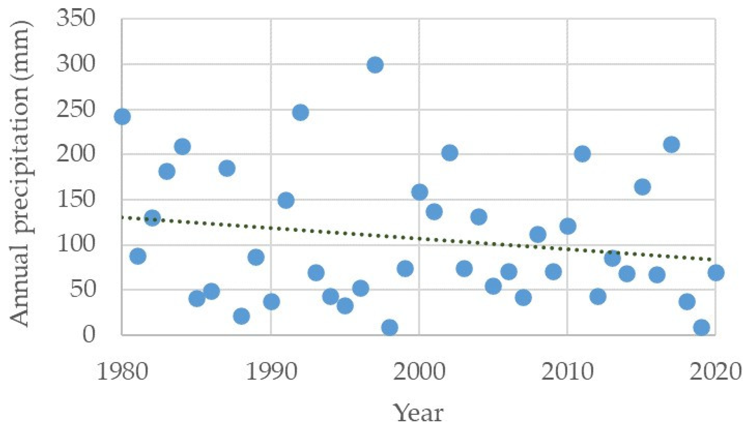
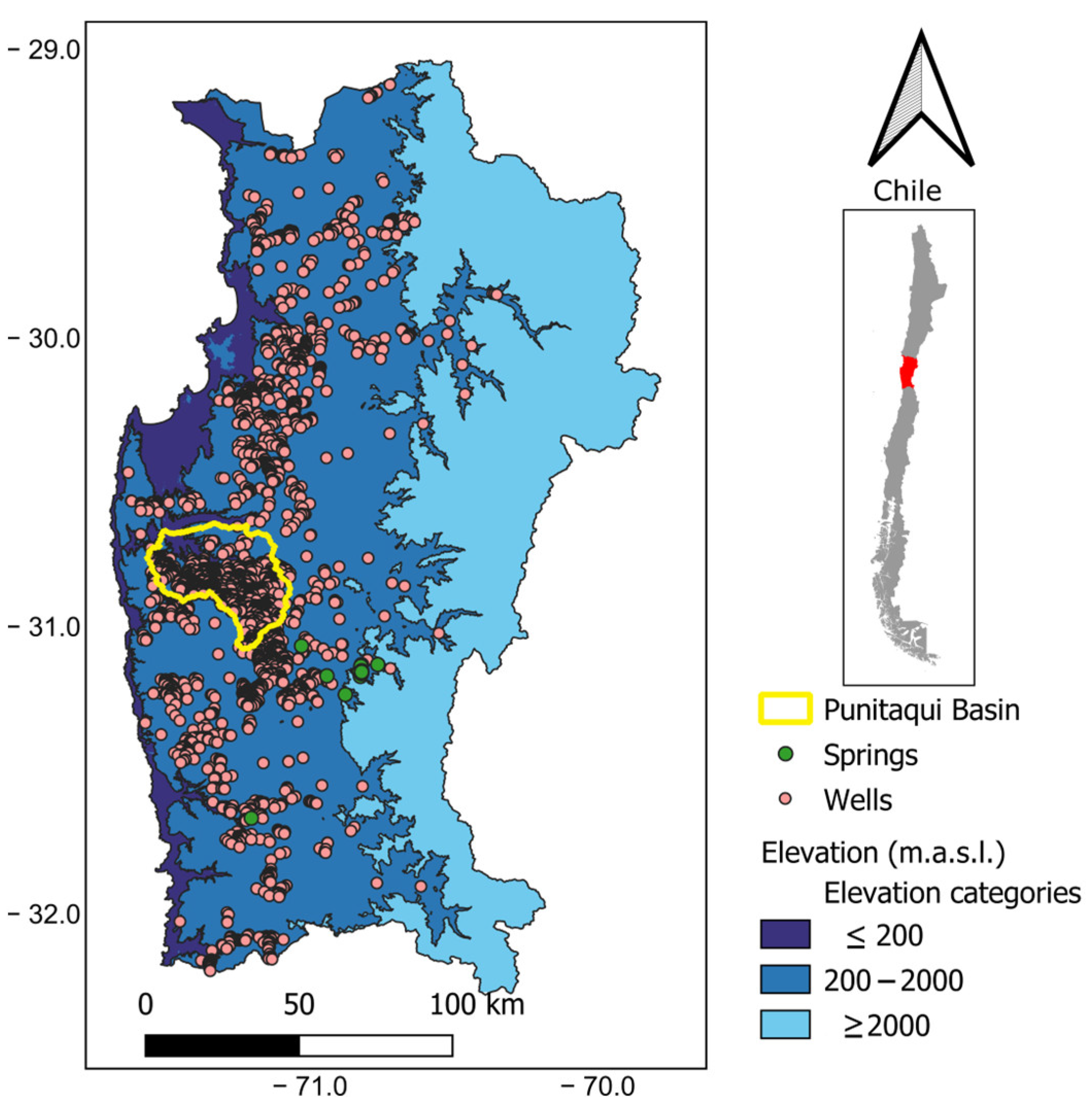
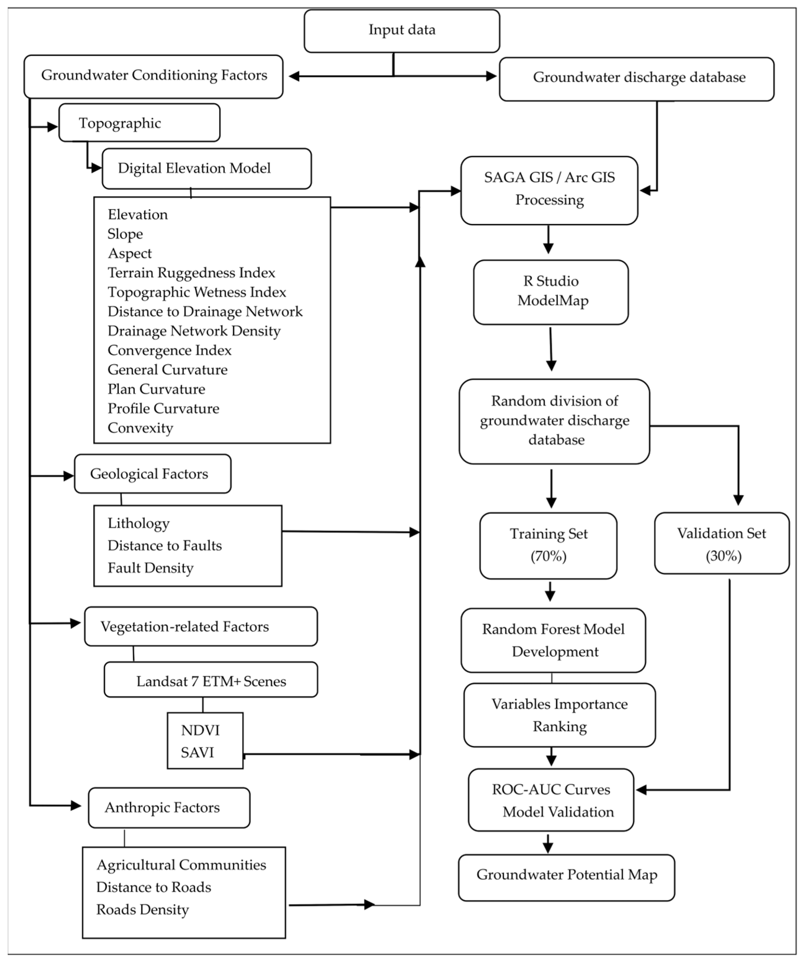
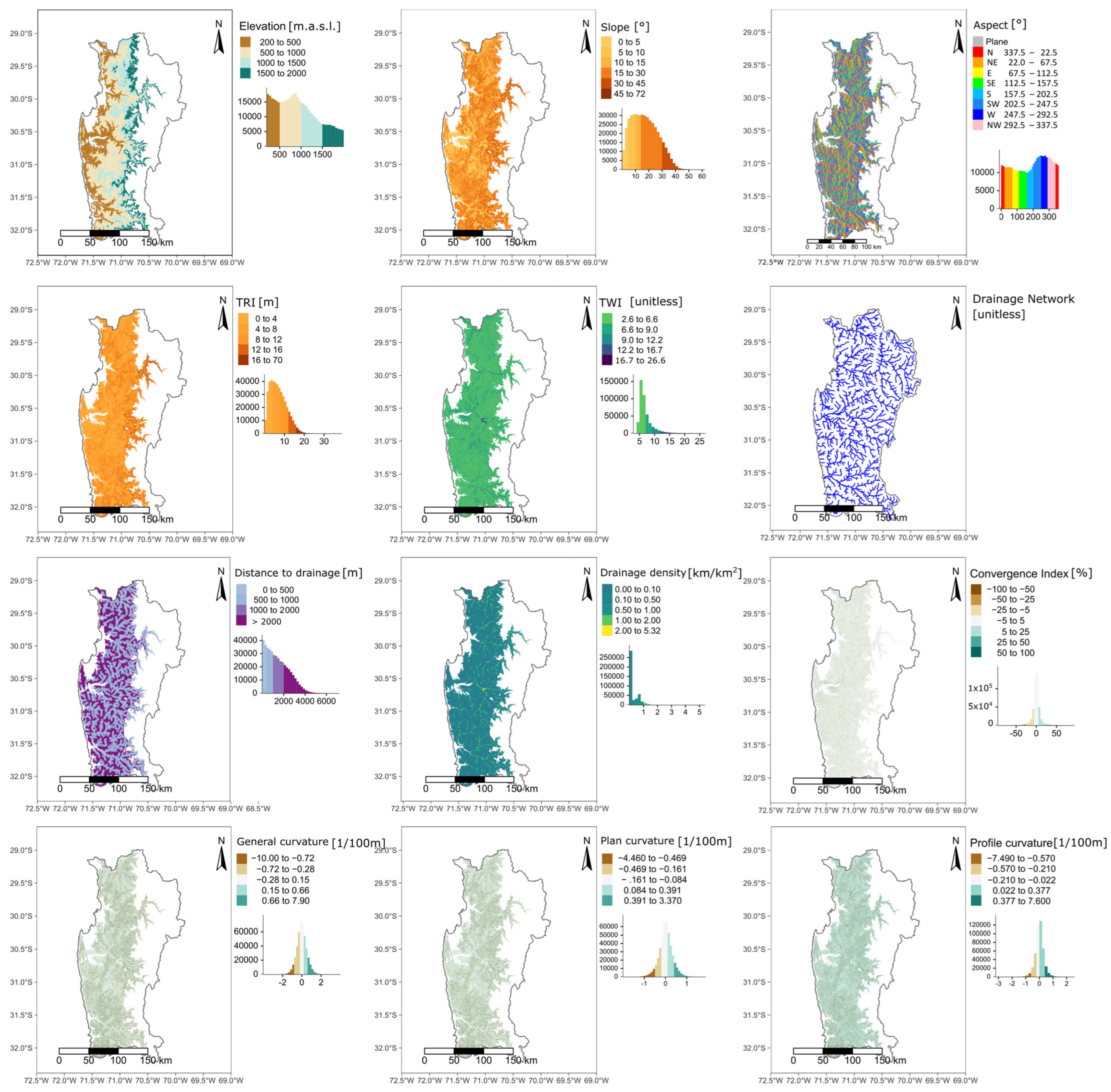
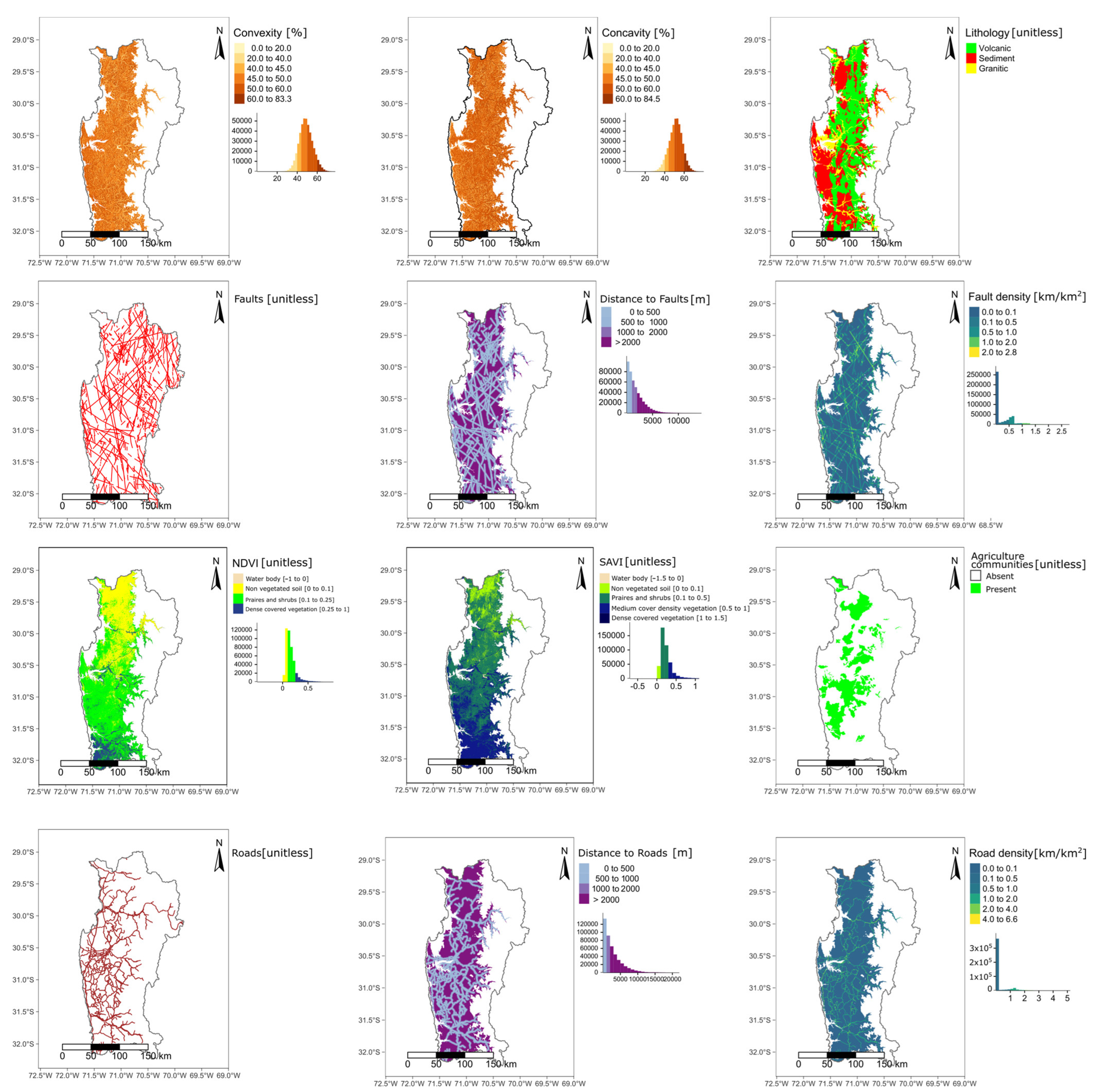
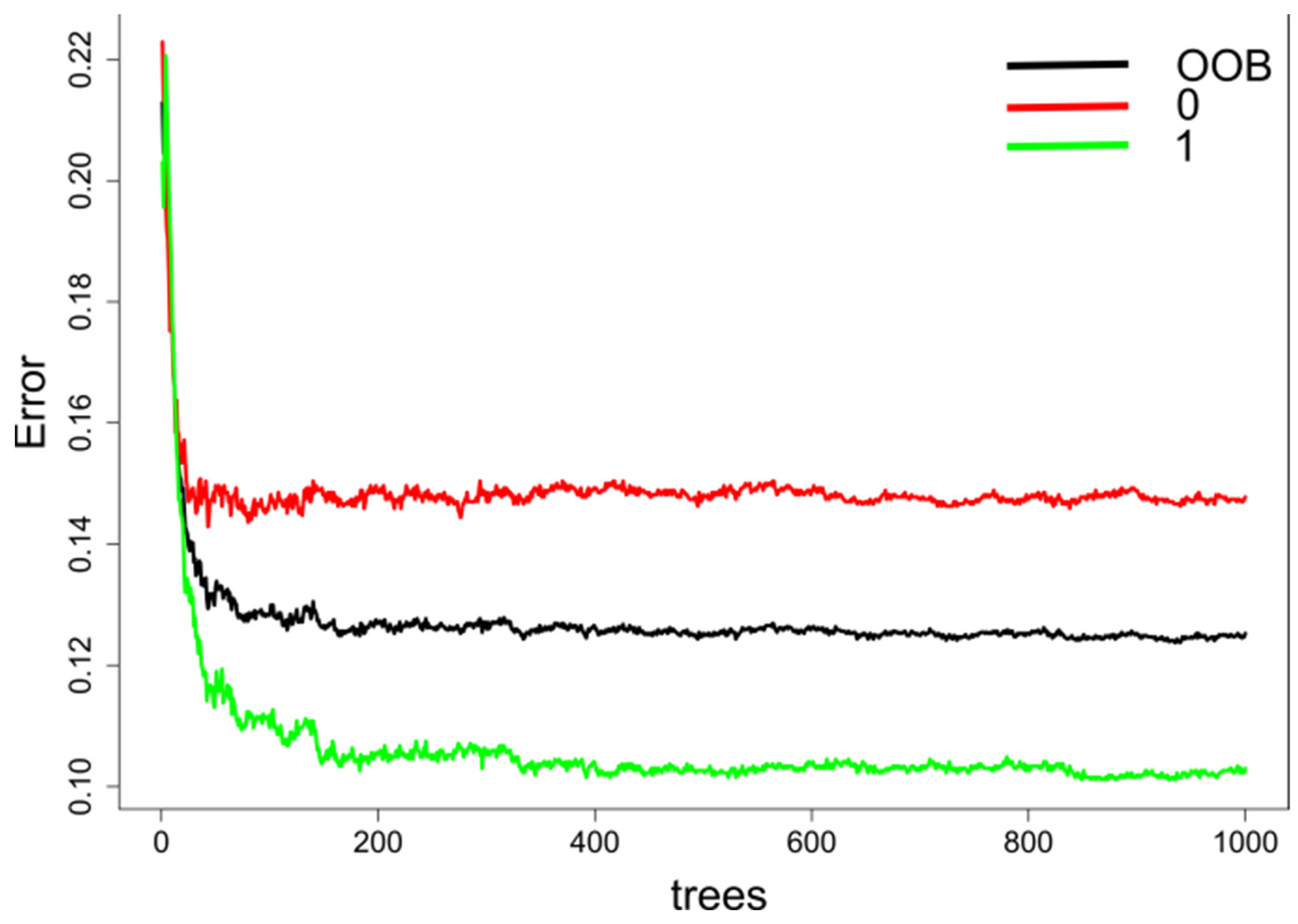
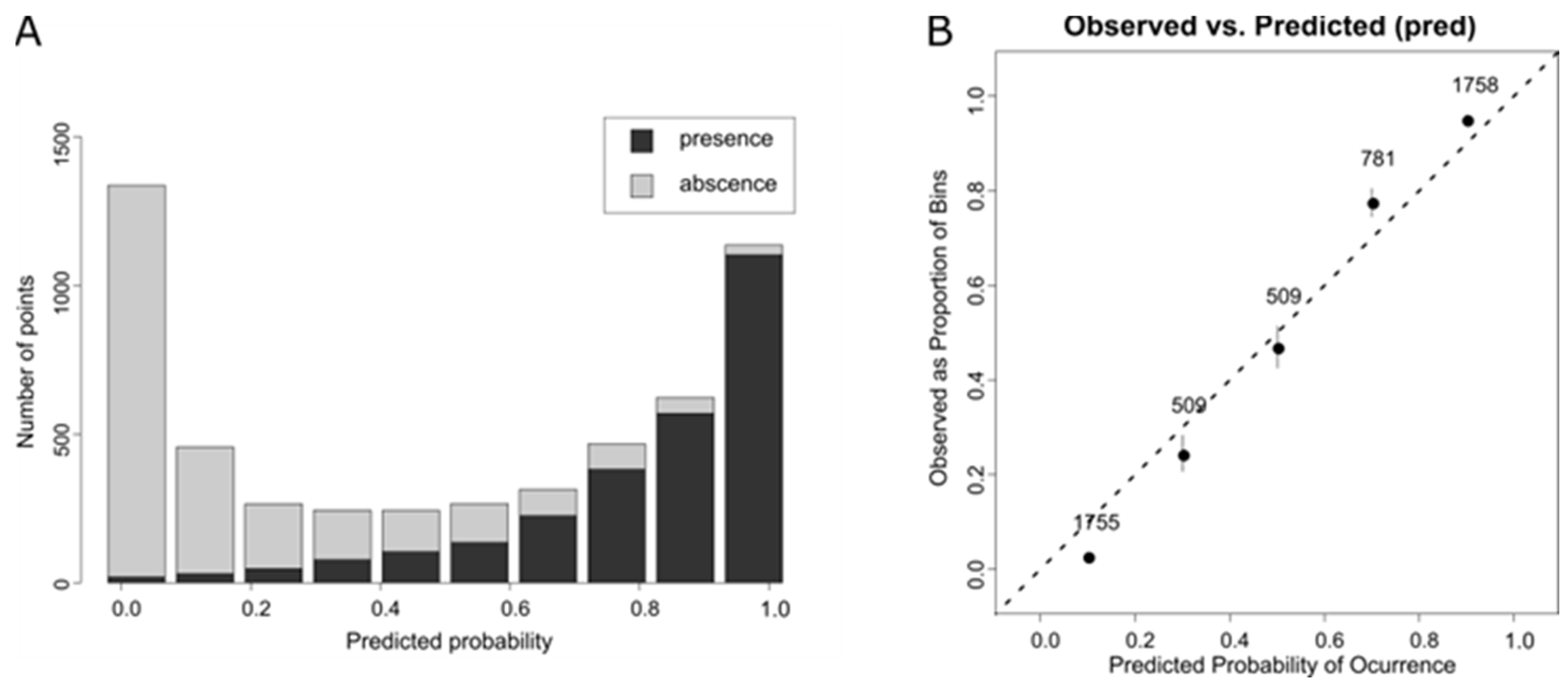
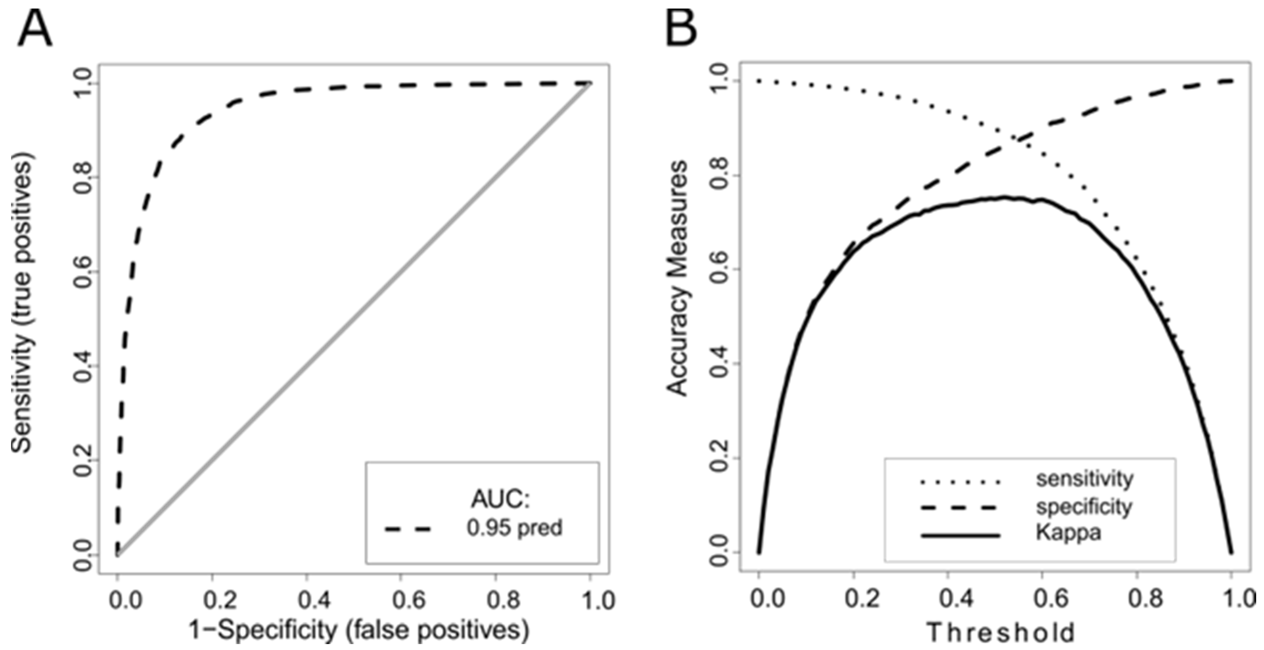
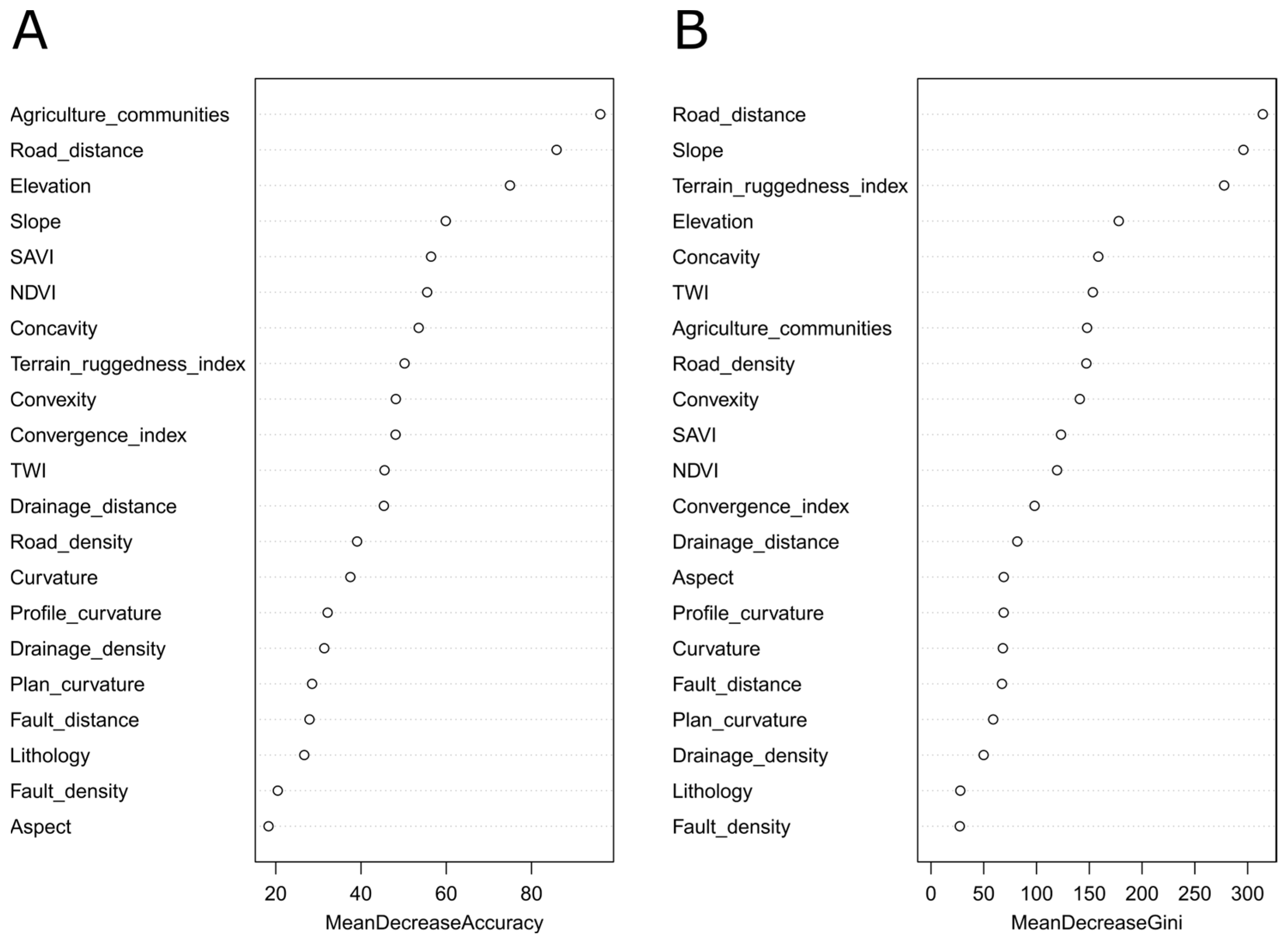
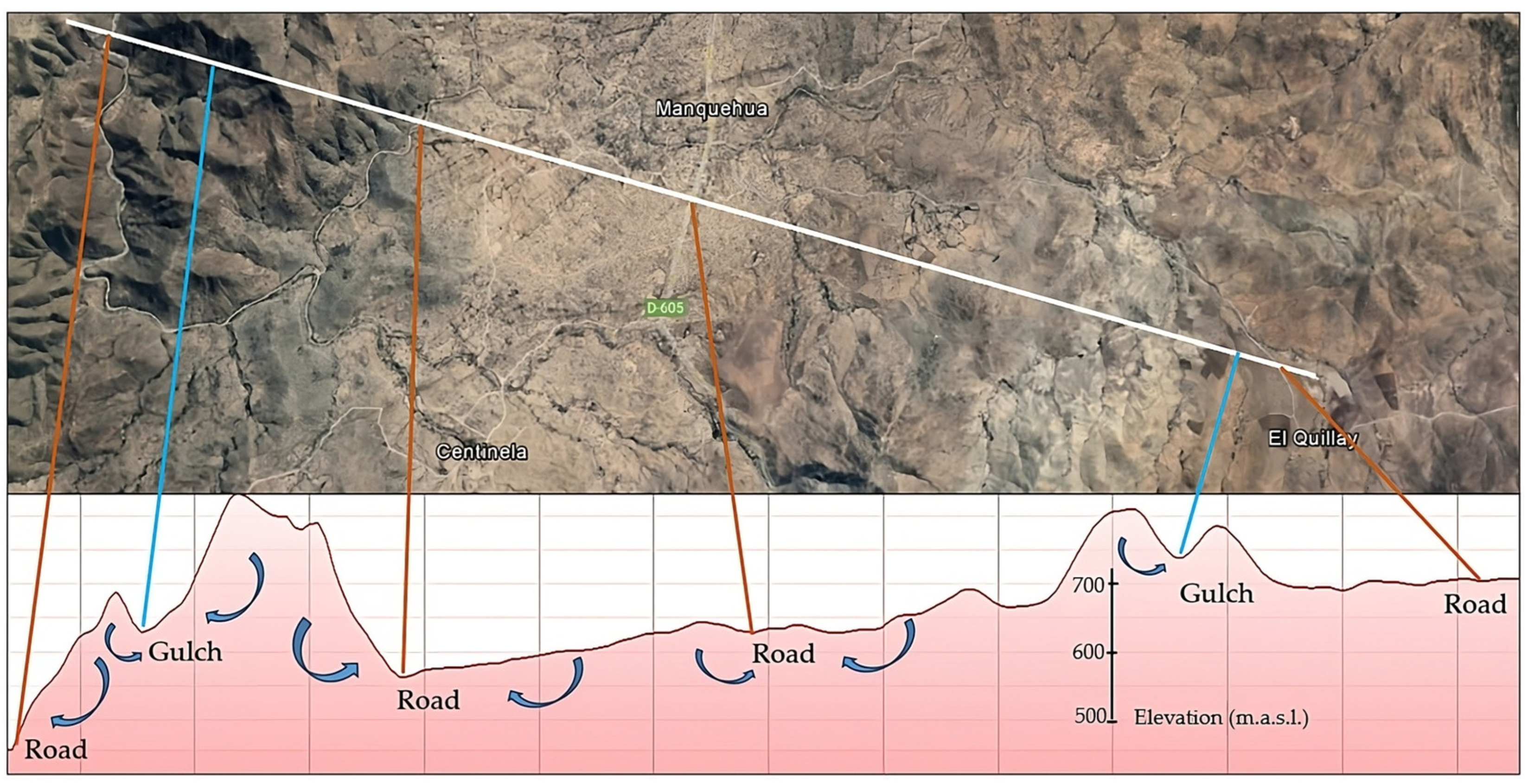
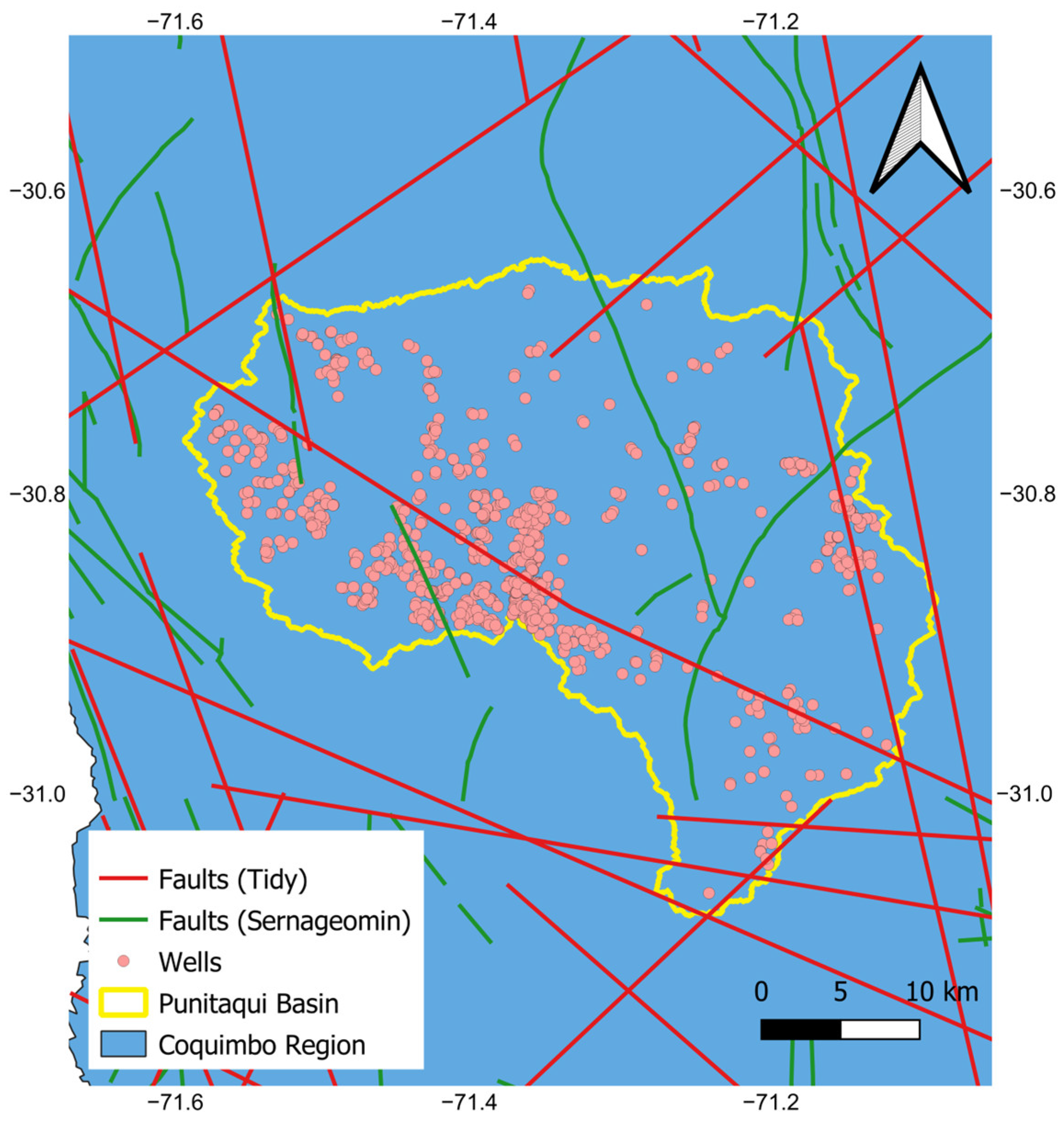
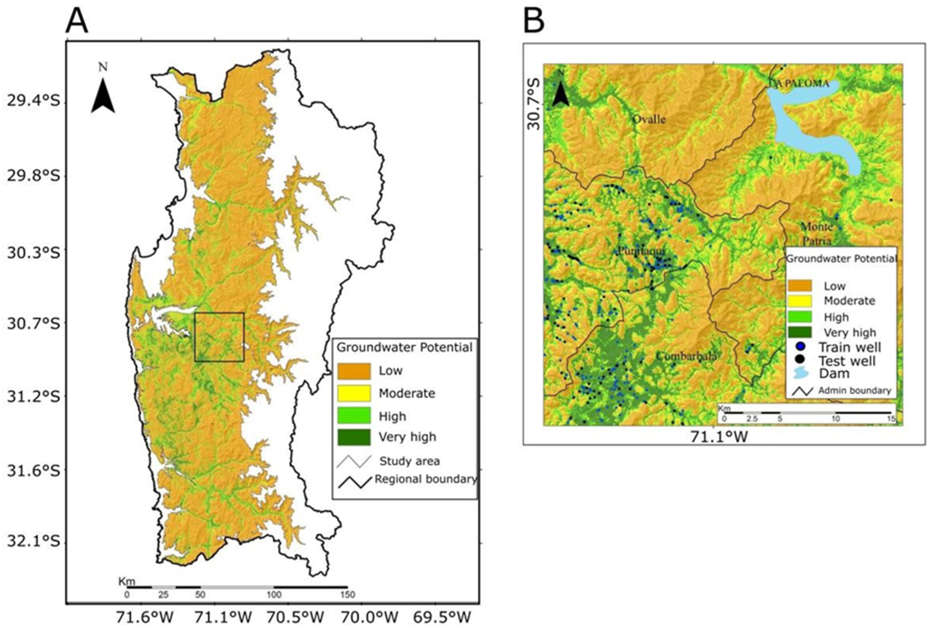


