1. Introduction
Unlined dam spillways and other hydraulic safety structures, such as sluice gates, stilling basins, and plunge pools, protect dam infrastructure during high water events. Dam safety can be improved by studying the hydraulic erodibility of these structures and the hydraulic characteristics of flowing water over these constructions. Erodibility, scour, and hydraulic erosion are technical terms related to the erosion that occurs when the hydraulic erosive intensity—erosive capacity of flowing water—exceeds the rock mass resistance [
1,
2].
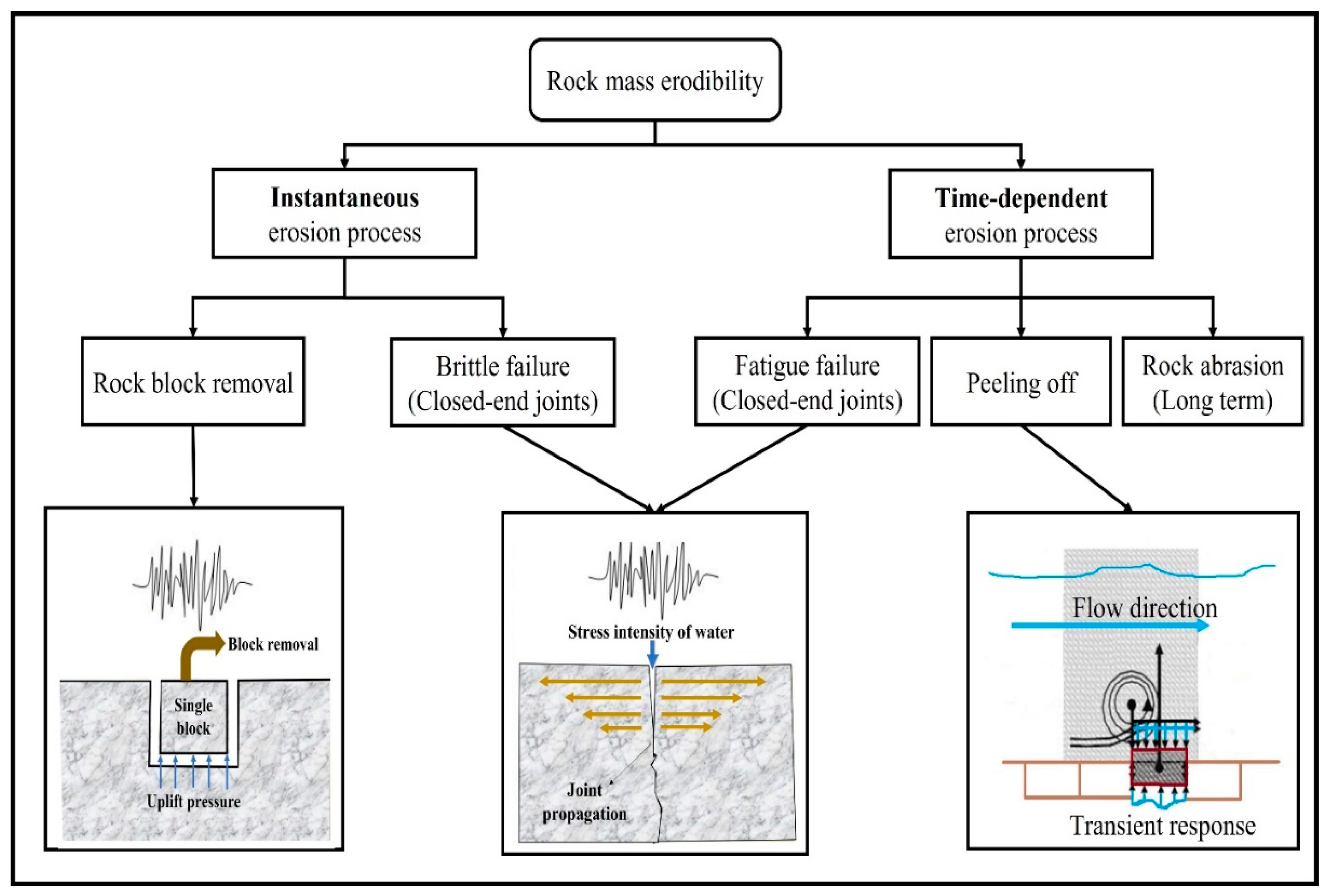
Rock mass erosion due to flowing water is a complex phenomenon that can occur instantaneously or over time. Hydraulic erosion mechanisms include brittle failure, fatigue failure, rock block removal, peeling off, and rock block abrasion (
Figure 1).
Both the hydraulic and rock mass aspects of erosion must be considered. Studying the effect of various geometries of hydraulic constructions on the hydraulic characteristics of flowing water and the effect of geomechanical parameters of the rock mass can improve the analysis of hydraulic erosive parameters [
5]. Several investigations have identified the unit stream power dissipation of water (Π
UD), water velocity (
V), shear stress (
τb) applied to a rock surface, stress intensity (
KI), and lifting force (
FL) as important hydraulic erosive parameters (
Table 1).
Most hydraulic erodibility assessments use an energy dissipation index to reflect the erosive capacity of water because of a lack of an accurate index and the difficulty in determining a specific erosive parameter [
6,
7,
8,
9,
10]. An energy dissipation index is selected for simplicity, not for accurately representing the hydraulic erosive agent (
Table 1). Pells’ (2016) analytical methodology appears to be the most reliable among the approaches that use energy dissipation as a hydraulic erosive agent. However, a measure of energy dissipation may not consider all the complexities involved with erosion; for example, spillway geometry (surface profile) and flow modes potentially influence the energy dissipation of water and erosion potential.
Average water velocity is not a representative index of the hydraulic erosive parameter because it depends on the flow channel surface profile, fluid viscosity, and flow nature. Average shear stress along the channel bottom can also be considered a hazard parameter. Nonetheless, it is extremely difficult to resolve all erosion problems within dam spillways by solely considering shear stress, including explaining hydraulic erosion caused by dynamic block removal, brittle failure, or fatigue failure.
Bollaert [
11,
12] proposed a comprehensive scour model (CSM) using three methods: a comprehensive fracture mechanics (CFM) approach for analyzing erosion in close-ended joints; a dynamic impulsion (DI) approach for analyzing erosion in open-ended joints (single block); and the quasi-steady impulsion (QSI) approach for computing the scoured depth along plunge pool walls. In the CFM, stress intensity (
KI) is considered a hydraulic erosive parameter and is calculated based on the maximum pressure at the plunge pool bottom. Bollaert’s DI considers uplift force to be a hydraulic erosive parameter on the basis of impulsion and Newton’s second law of thermodynamics. This method ignores the geomechanical and geometric characteristics of the rock mass. In the DI approach, it is assumed that the shear force (
Fsh) is zero. Bollaert’s QSI method determines the forces applied to channel bottoms through the quasi-steady lift force (
FQSL) on a protruding block, where the
FQSL is dependent on uplift pressure and flow velocity.
Various studies significantly advance our understanding of turbulent fluid dynamics near rough walls. Schmidt and Schumann’s 1989 research deeply investigates turbulence within a convective boundary layer (CBL), utilizing large-eddy simulations across various roughness heights. This inquiry integrates finite-difference integration of Navier-Stokes equations, comparing outcomes with empirical data and revealing alignment in vertical mean turbulence metrics, while highlighting differences in horizontal velocity oscillations, pressure perturbations, and dissipation rates [
13]. Similarly, Carlotti’s 2002 study employs large-eddy simulation (LES), rapid distortion theory, and Eulerian kinematic simulation to explore turbulence properties near the ground, revealing an inner boundary layer within an eddy surface layer, analyzing streamwise structures, spectral signatures, vertical correlations, and spectrum slope modifications [
14]. In 1976, Townsend extensively investigates the intricate dynamics underpinning turbulent shear flow, unveiling chaotic behaviors driven by velocity gradients within the fluid [
15]. While inspiring, it is vital to recognize that these studies may differ in terms of roughness scales and fluid mechanics contexts from our project. This contrast fuels the development of a tailored, accurate model for our unique project scenario. Together, these scholarly endeavors deepen our understanding of diverse turbulence manifestations.
Existing methods of assessing and predicting hydraulic erodibility are limited by several elements, and these approaches can be used only in specific situations and conditions. Moreover, a unique parameter is lacking to measure the erosive agent of water when assessing rock mass erodibility. For example, numerous equations exist for determining the unit stream power dissipation of water (Π
UD)—initially developed using internal flow conditions. The concept of stress intensity (
KI) was originally developed for metallurgical analysis [
11] and is only used to estimate the probability of joint propagation in intact rocks, not rock masses. When the existing methods are compared (
Table 1), the stream power dissipation parameter is the most commonly used; however, spillway geometry is not considered.
Table 1.
Existing hydraulic erosive indices.
Table 1.
Existing hydraulic erosive indices.
| Hydraulic Erosive Parameter | Equation |
|---|
| Parameter | Approach |
|---|
|
Unit stream power dissipation (ΠUD) and Stream power dissipation (ΠD)
| (Van Schalkwyk 1994) [10] | |
| (Annandale 1995) [6] | |
| (Pells 2016) [1] | |
|
Velocity (V)
| (Weisbach 1845, Darcy 1857) [16,17] | |
| (Manning et al., 1890) [18] | |
|
Shear stress (τb)
| (Yunus 2010) [19] | |
|
| MPM (Khodashenas and Paquier 1999) [20] | |
| (Prasad and Russell 2000) [21] | |
| (Yang and Lim 2005) [22] | |
| (Guo and Julien 2005) [23] | |
| (Seckin, Seckin et al., 2006) [24] | |
| (Severy and Felder 2017) [25] | |
|
Stress intensity (KI)
| Bollaert and Schleiss 2002) [11] | |
|
Lifting force (FL)
| (Bollaert and Schleiss 2002) [11] | |
| (Bollaert 2010) [12] | |
After extensive analysis and investigation of dam construction projects, with a specific focus on hydraulic erosion within unlined spillways and its pivotal role in dam construction, the decision was taken to deeply explore this matter. Previous research concerning methodologies for assessing hydraulic erosion in dam spillways has shed light on the strengths and limitations of various approaches:
- (1)
Semitheoretical Approaches: Notably, Pells’ RMEI method among semitheoretical approaches showcased relatively lower errors compared to counterparts within the same category, despite inherent margins of error.
- (2)
Semianalytical Methods: Among the array of semianalytical methods, Bollaert’s CSM approach emerged as a representative choice for evaluating hydraulic erodibility, particularly in scenarios involving plunge pool dynamics. The challenges associated with obtaining site-specific data were balanced by its applicability to channel flow situations, thereby suggesting its potential as a novel analytical technique tailored for unlined spillways.
- (3)
Advancing Erosion Prediction Methods: The significance of developing new or refining existing erosion prediction methods was underscored as crucial for dam spillway design. This endeavor addressed the following pivotal aspects:
Distinct Hydraulic Erosive Parameter: A foundational step involved defining a distinctive hydraulic parameter.
Dam Spillway Geometry Influence: The influence of dam spillway geometry on the hydraulic erosive parameter.
Impact of Rock Mass Geometry: Delving into the implications of rock mass geometry, including factors like block volume, joint characteristics, dip, and dip direction, on the hydraulic erosive parameter.
Geomechanical Scrutiny: Definition of the effects of geomechanical factors on the hydraulic erosive parameter.
With the recognition that hydraulic erodibilty within unlined spillways encompasses both hydraulic and geomechanical aspects, this phenomenon is studied to encompass both aspects. Given the industry’s reliance on established approaches like the Annandale methodology, the initial focus was directed toward the hydraulic aspect. This article stands as an important part of a comprehensive study on introducing a holistic framework for assessing hydraulic erosion. This phase concentrated on examining the influence of geometric parameters on hydraulic parameters, setting the stage for future exploration into the interplay of geomechanical parameters with hydraulic properties. This study specifically undertook a meticulous examination of the effects of geometric parameters, with a specific emphasis on rock surface irregularities, on hydraulic parameters. The new findings provided the basis for introducing the comprehensive methodology for assessing hydraulic erodibilty. Future research phases will delve into the influence of geomechanical parameters on hydraulic parameters. Combining the knowledge accumulated from these phases will result in the development of a distinctive equation for the hydraulic erosive parameter. The ultimate objective is to present a comprehensive and coherent methodology for evaluating hydraulic erosion within unlined dam spillways.
In the article, various unlined spillway surface geometries were investigated to determine how hydraulic parameters are affected by irregularities on unlined spillway surfaces. A series of geometries found in unlined spillways were selected, and flow simulations were performed using computational fluid dynamics (CFD) with ANSYS-Fluent software. ANSYS-Fluent was chosen based on its industry-standard recognition, versatility in handling complex simulations, user-friendly interface, and robust solver options, all of which were aligned with the research requirements. These simulations were two-dimensional (2D) and were solved as steady-state flows. Within turbulent model simulations, the intricacies of irregular rock surfaces were explored—a pursuit characterized by challenges and significance. The chosen approach encompassed the utilization of the k-epsilon turbulence model with Explicit Enhanced Wall Treatment, which proficiently managed the complexities arising from surface roughness. Beyond being a necessity, the drive for accuracy assumed the role of a conduit for informed decision-making. Central to the methodology was the reliance on y+ values, serving as evaluative measures. Their impact extended to the refinement of the model and the adaptation of mesh sizes by the computed y+ values. The alterations in hydraulic parameters, including pressure (total pressure), shear stress, flow velocity, and energy, were then determined based on spillway surface geometry, i.e., irregularity height (h) and irregularity angle (α1).
2. Materials and Methods
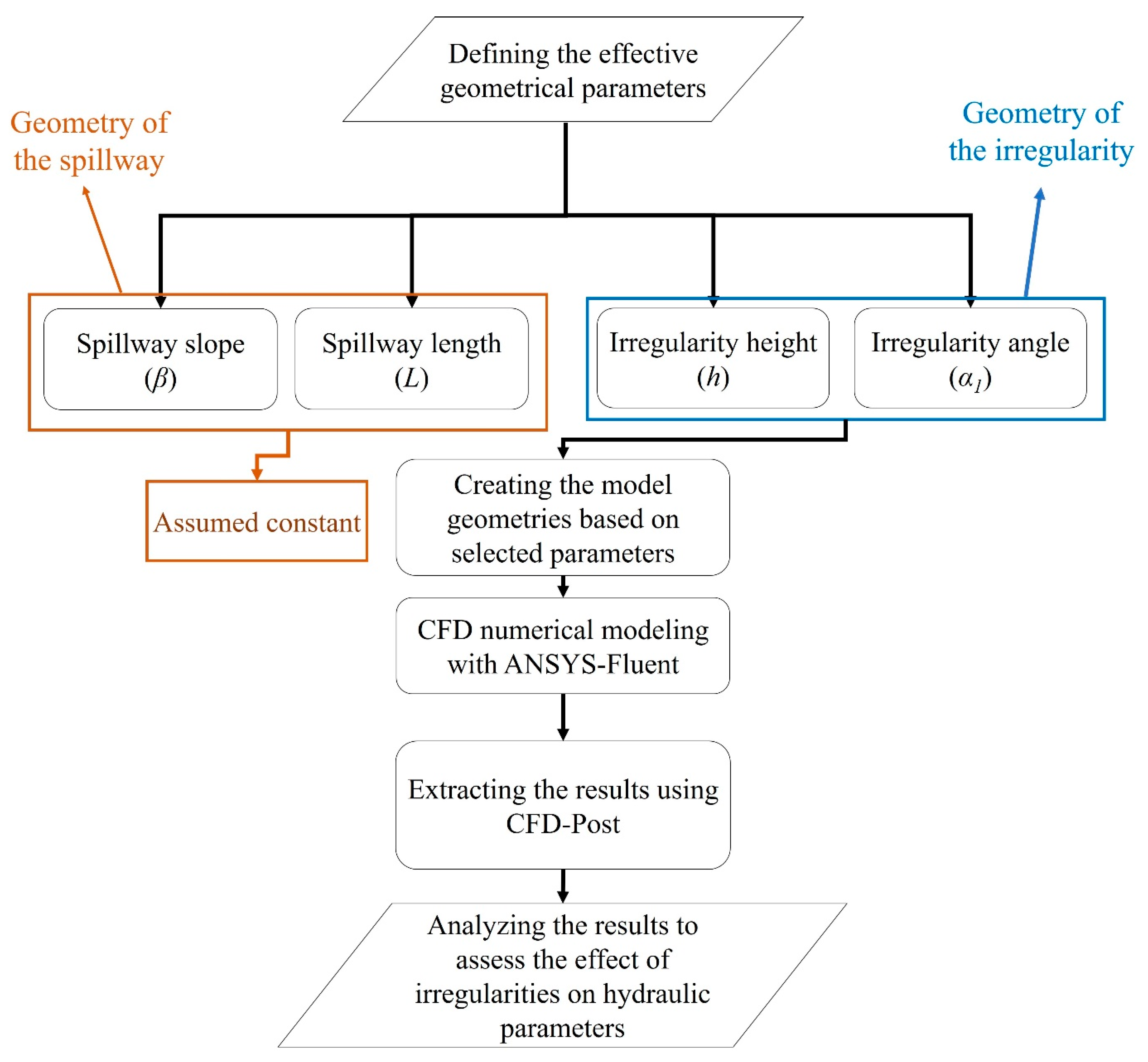
The flowchart of the methodology (
Figure 2) presented the steps in subsections. The most effective geometric parameters of spillways and irregularities were first identified and selected by analyzing the available data from Pells [
1]. Pells’ data involve more than 100 case studies from dams in Australia, Africa, and the United States [
1].
These selected parameters combined with observed controlled blasting patterns and available data resulted in a specific model geometry. Then, water flow over this rock geometry was simulated using ANSYS-Fluent software, and the results were extracted using CFD-Post.
The spillway geometric parameters, including spillway length and constant spillway slope, and the geometric parameters of the irregularities, including their length, height, and angle, will be explained in
Section 2.1.
The purpose of this study is to provide a foundational understanding of hydraulic erosion science. This phenomenon was characterized by the synergy of hydraulic and geomechanical principles. Parameters in this science were categorized into three main groups: hydraulic, geomechanical, and geometric:
Hydraulic parameters included total pressure, shear stress, flow velocity, force, stream power, and energy.
Geomechanical parameters encompassed block volume, joint aperture, dip angle, and dip direction.
Geometric parameters involved the shape of the rock surface, slope, and channel structure.
Given the complexity, these parameters will be analyzed separately. The focus was directed towards examining how geometric attributes, specifically the length (l), height (h), and angle (α1) of rock surface irregularities, impacted hydraulic parameters. With the value of l held constant (given its direct relationship with other geometrical parameters), the focus was exclusively directed towards h and α1. The investigation primarily centered on hydraulic parameters such as velocity, pressure, force, and energy. These parameters played a pivotal role, as they affected a range of other factors. By exploring the influence of h and α1 on these hydraulic parameters, insights were gained into broader interactions.
Subsequent research delved into the impact of the remaining geometric and geome-chanical factors on hydraulic parameters. Ultimately, the aspiration is to develop a comprehensive equation that integrates all attributes, offering a unified perspective on the science of hydraulic erodibility.
2.1. Determining Model Geometry
The effects of each parameter were considered separately due to the high number of variables. For this paper, only the results of irregularity height (h) and angle (α1) are presented.
2.1.1. Step 1: Blasting Effect on the Profile of Surface Irregularities
In the context of mining, tunnelling, and dam construction, blasting is a common method of breaking and removing rock mass. In mining and tunneling operations, the high levels of detonation energy are emitted, a portion of which is productively expended on rock fragmentation [
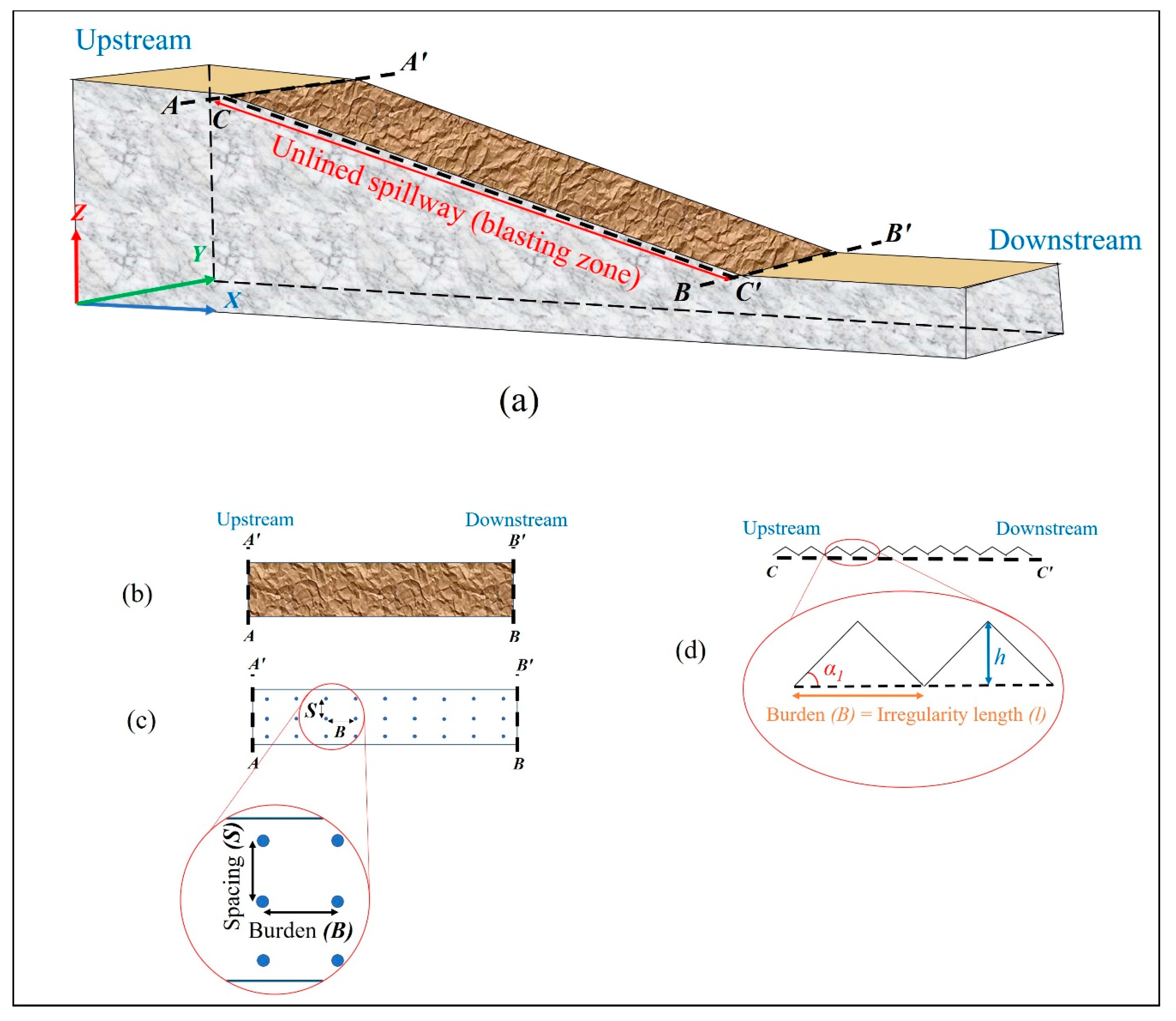
26]. Unlined dam spillways are generally built on hard rock, and controlled blasting is usually used to create the surface of the unlined spillways (
Figure 3). The applied drilling and blasting produce irregularities along a spillway’s surface profile [
27]. When designing blasting patterns for unlined dam spillways, burden (
B) and spacing (
S) are important (
Figure 3c). Burden denotes the distance between a blasting-hole row to the excavation face or between blasting-hole rows. Spacing refers to the distance between blasting holes along the same row [
27]. According to blasting theory, the burden for hard rocks is 1–2 m. Based on the blasting patterns and the created post-blasting surfaces, the burden was considered to be equivalent to irregularity length (
Figure 3d).
2.1.2. Step 2: Selection of Geometries for Unlined Surface Profiles
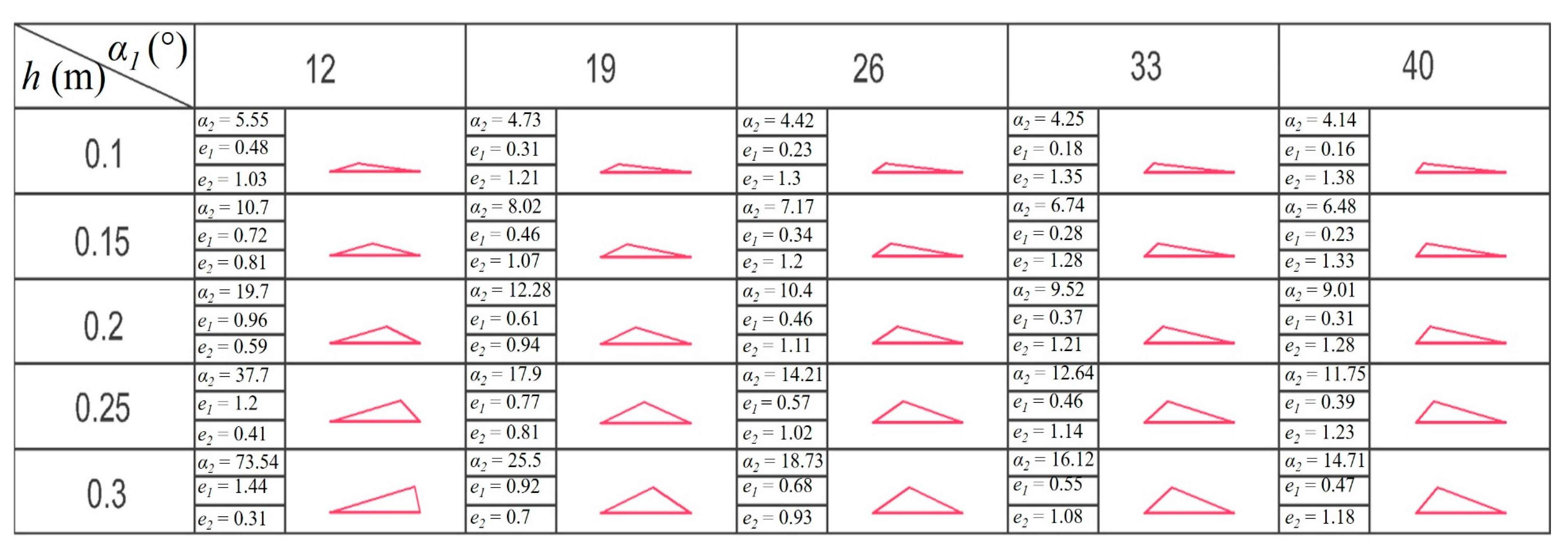
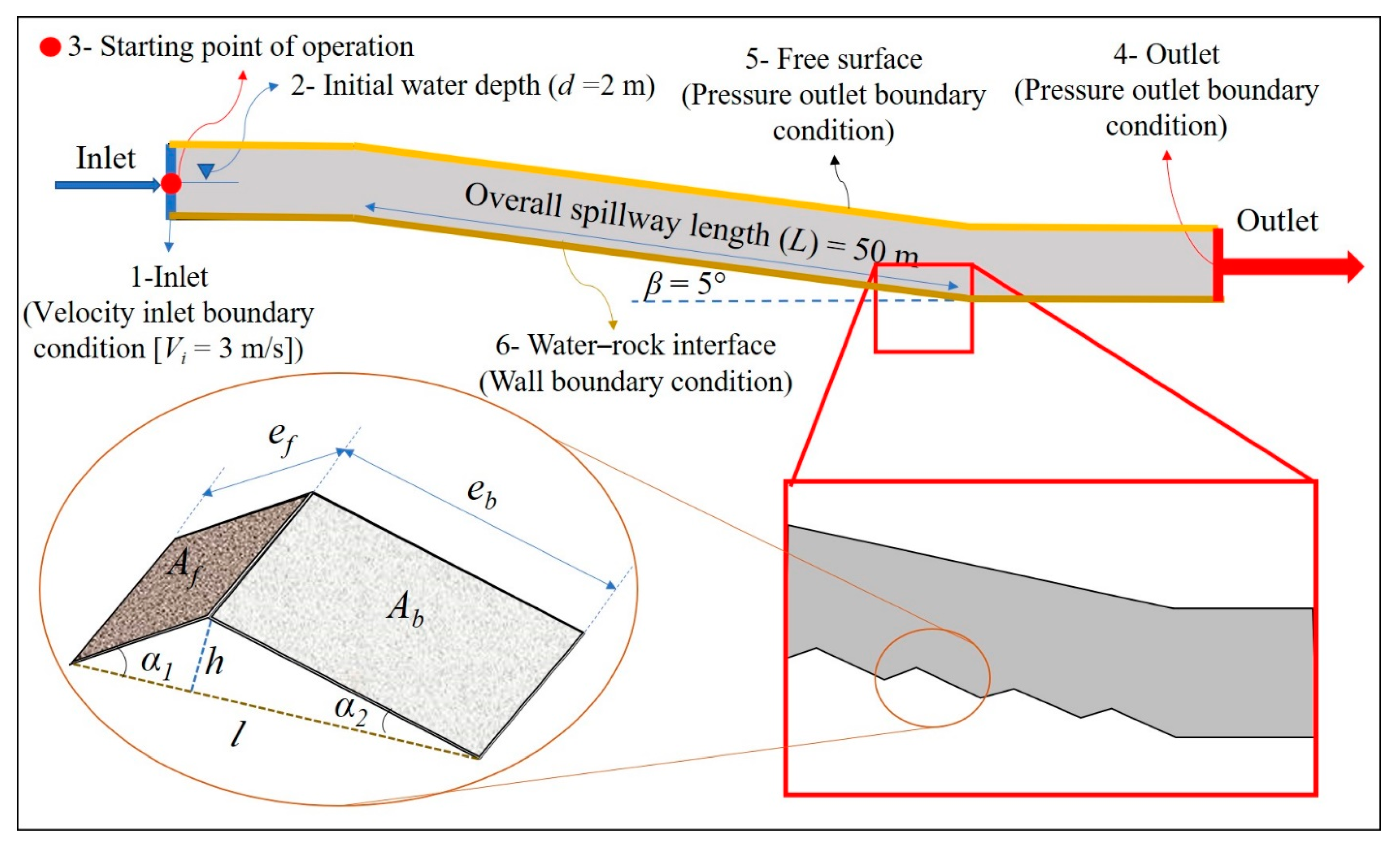
In this study, the spillway geometric characteristics of spillway length (L) and spillway slope (β) were considered, and the selected geometric parameters of irregularities comprised the length (l), height (h), and angle (α1) of the irregularities. It was assumed that the spillways’ geometric parameters remained constant. An irregularity angle ranging from 12° to 40° covered most irregularities, and the irregularity height varied between 10 and 30 cm. The irregularity length was proportional to the height and angles and generally fell between 1 and 2 m. A length of 1.5 m was selected for all the models.
The geometric characteristics of the spillway (slope and length) were also considered significant, and future studies aimed to evaluate the effects of these parameters. For the models, a profile angle of 5° and a length of 50 m were selected based on observations of unlined spillways, choosing the average values of these observations (
Figure 4). A total of 25 geometric configurations of spillway surface irregularities were produced.
To identify the geometric parameters of the irregularities, Equations (1)–(3) from geometry science were applied. These equations were a function of the input parameters, and the irregularity geometry could be created using these equations and the input parameters
α1,
h, and
l. The lengths of irregularity surfaces with and against water flow were represented by e
b and e
f, respectively (
Figure 4). The irregularity angle in the flow direction, along with the spillway slope, was known as
α2. This study considered several configurations, as shown in
Figure 5.
2.2. Numerical Modeling
To simplify the computation of wall parameters on irregular surfaces, ANSYS-Fluent Version 2020 R2 was used in this study. ANSYS-Fluent converts scalar transport equations into algebraic equations that can be run numerically on the basis of a controlled volume approach. Functioning within a 2D framework, the CFD model was employed to solve under steady-state conditions. This configuration allowed for a focused examination of essential fluid dynamics aspects. The objective behind these simulations was to capture the sensitivity of hydraulic parameters to irregularities present on the rock surface. The open-channel submodel in ANSYS-Fluent, partially based on the volume of fluid (VOF) multiphase model, was used in the analysis [
28]. In the original VOF technique, Hirt and Nichols [
29] used a specialized methodology to obtain a standard definition of the free surface, whereas ANSYS-Fluent solves the combined air–water flow systems [
30]. In the realm of turbulent model simulations, the investigation of irregular rock surfaces emerges as both a challenge and an avenue of significance. The selected path involves employing the k-epsilon turbulence model with Enhanced Wall Treatment, a strategic choice well-suited for addressing the intricacies arising from surface roughness. This approach, motivated by the pursuit of accuracy as a foundation for informed decision-making, hinges on the pivotal role of y+ values. Y+ values, acting as evaluative indicators, play a crucial role in refining the model and adjusting mesh sizes. Serving as a touchstone for near-wall resolution in turbulent simulations, y+ values enable the calibration of the model’s mesh. This calibration, guided by the computed y+ values, fine tunes the mesh sizes, ensuring a harmonious fit that mirrors real-world intricacies accurately. Within the framework of k-epsilon turbulence modeling, precise alignment with y+ values not only rectifies errors arising from improper meshing but also creates a simulation environment faithfully capturing the physics near rough wall interfaces. Incorporating the y+ value and executing grid convergence analysis on several parameters, endeavors were made to confine them within the range of 1 < y+ < 30. Following successive iterations of mesh refinement and subsequent reduction, the y+ value was progressively brought to an approximate range of 30. The accuracy of the model was subsequently evaluated through rigorous grid convergence analysis, closely associated with the y+ values.
Solutions to the Navier–Stokes equations were derived using a stable, implicit technique in the simulations. Pressure–velocity coupling was treated for stability using the widely used COUPLED method. To enhance momentum, a second-order upwind scheme was applied in this study.
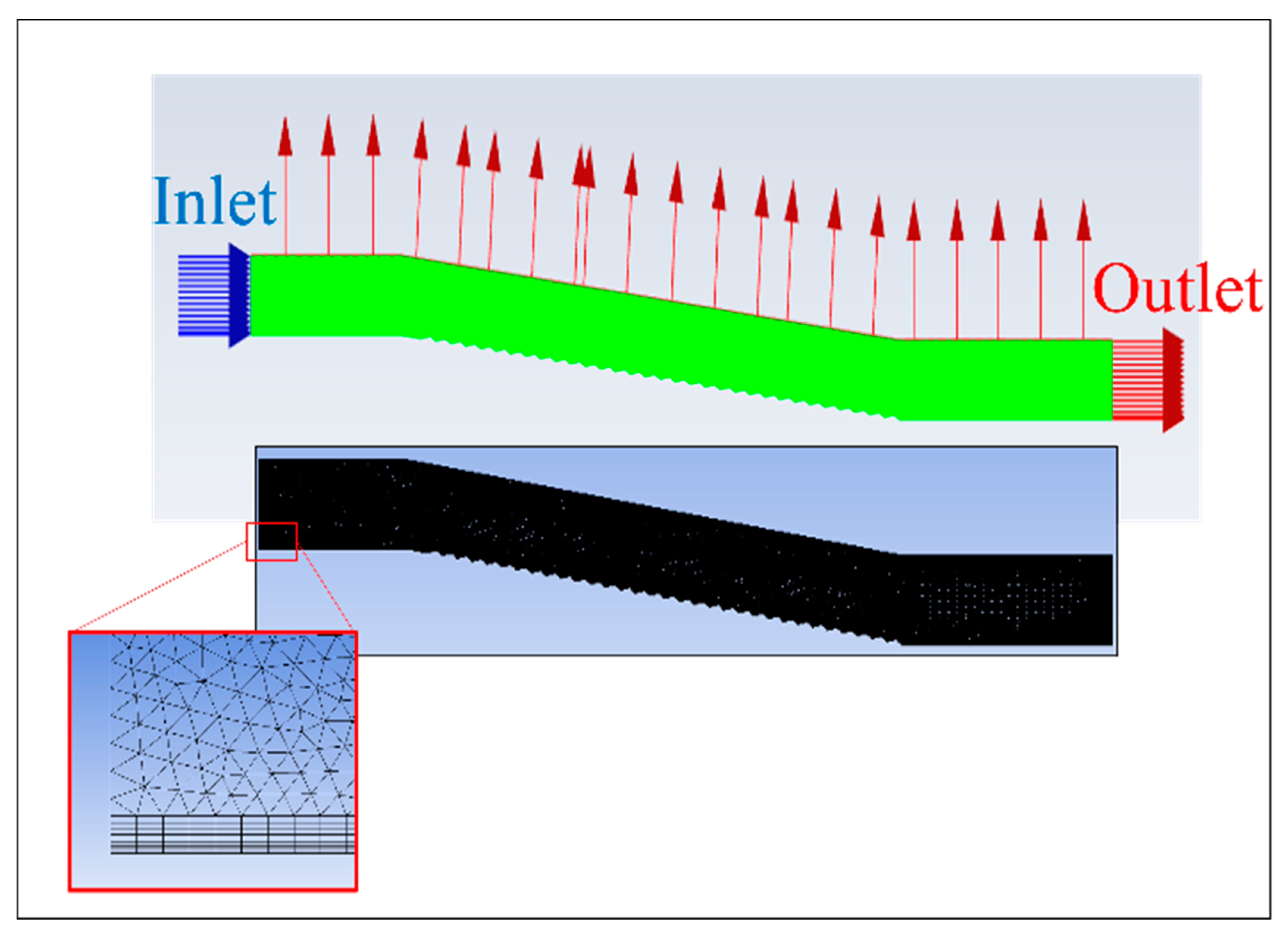
Table 2 presented the model input data for the fluid flow modeling. A 3 m/s velocity-inlet boundary condition was applied. In open channels, upstream velocity–inlet boundary conditions define the flow velocity and relevant scalar characteristics of the flow at the flow inlet. At the outflow zone, a pressure–outlet boundary condition was specified. A no-slip boundary condition was assumed at the water–rock interface (
Figure 4). The water depth at the model’s entrance (inlet) was the starting point for the simulation calculations. Atmospheric pressure and a 2 m water depth were also set in the model.
Figure 6 shows the produced model in ANSYS-Fluent and the meshing used. To avoid the impact of localized bursts, it was effectively mitigated by the employed mesh refinement strategy, thereby enhancing the fidelity of CFD simulations. The ultimate aim was to attain an optimum simulation model that harmonized accuracy and cost-effectiveness.
2.2.1. Step 1: Model Geometry and Boundary Conditions
Designing the geometry is the first step of
CFD numerical modeling. Therefore, various simulation geometries were produced using the ANSYS geometry tool. Five irregularity heights (
h) and five irregularity angles (
α1) were identified based on the Pells data set. A total of 25 configurations were considered for this study (
Figure 5).
2.2.2. Step 2: Meshing and Convergence Analysis
In the research, the physical model was mesh-constructed using a triangular structural grid. An inflation layer was applied along the spillway wall, and the mesh gradually increased in size from bottom to top to provide a more accurate simulation that captured the boundary layer. At the channel bottom, five inflation layers with a growth rate of 1.2% were considered.
To determine whether the precision of the numerical simulations was affected by grid cell size—and to find the optimal grid size—the first branch–channel physical model was meshed using five distinct techniques (the maximum grid cells were 20, 15, 10, 5, and 1 cm). This analysis was conducted for the final irregularity along the spillway, and the results were evaluated in terms of total pressure, maximum velocity, and water depth for
h = 10 cm and
α1 = 12°. A meshing size of 10 cm was deemed optimal on the basis of outcomes of this grid convergence analysis (
Table 3), considering the criteria of the time calculation and precision of the results. Finally, an approximately 48 m long portion of the channel (CC’ red line in
Figure 3a) was analyzed.
2.2.3. Step 3: Model Setup (VOF Method, Turbulence Model, Control Equation)
Free surface channel fluctuations impact both the air and water phases and complicate the modeling. By resolving a single momentum equation and storing a record of the volume fraction of each immiscible fluid inside the computational region, the VOF model can simulate two or more immiscible fluids. Moreover, the VOF approach can be applied to a wide range of discontinuous interfaces and flowing water and allows monitoring the water surface in open channels. The sum of all volume fractions of all phases in each control body is one [
31].
where
and
represent the volume fractions of water and air, respectively. When
aw = 1, water fills every control unit in the calculation domain, and when
aa = 1, it fills with air. Tracking the air–water interaction requires the following continuity equation [
32]:
where
Xi represents the coordinate and
ui denotes the flow velocity. (For units of the various parameters, please refer to the included symbol notation table)
Both the continuity and momentum equations for a free and incompressible fluid in an open channel can be expressed as
where
V is the flow velocity,
u and
v are the velocity components of fluid particles in the 2D spatial directions
x and
y,
ρ is the density of water,
is the dynamic viscosity,
P is the pressure
(Pa), and
Fu and
Fv are the forces of fluid particles in 2D directions.
The RNG k-ϵ turbulence model eliminates average flow rotation and whirling by modifying turbulent viscosity. The related equation is [
33]
where
k denotes the turbulent kinetic energy,
ϵ represents the turbulent energy dissipation rate, μ expresses the hydrodynamic viscosity coefficient,
Gk denotes the turbulent kinetic energy production term,
represents the effective dynamic viscosity coefficient
and
denote the constants 1.42 and 1.68, respectively.
3. Results
The effect of surface irregularity on pressure, stress, flow velocity, and energy were evaluated under 25 different irregularity configurations. In the following subsections, the effects of irregularities on the hydraulic parameters are examined independently.
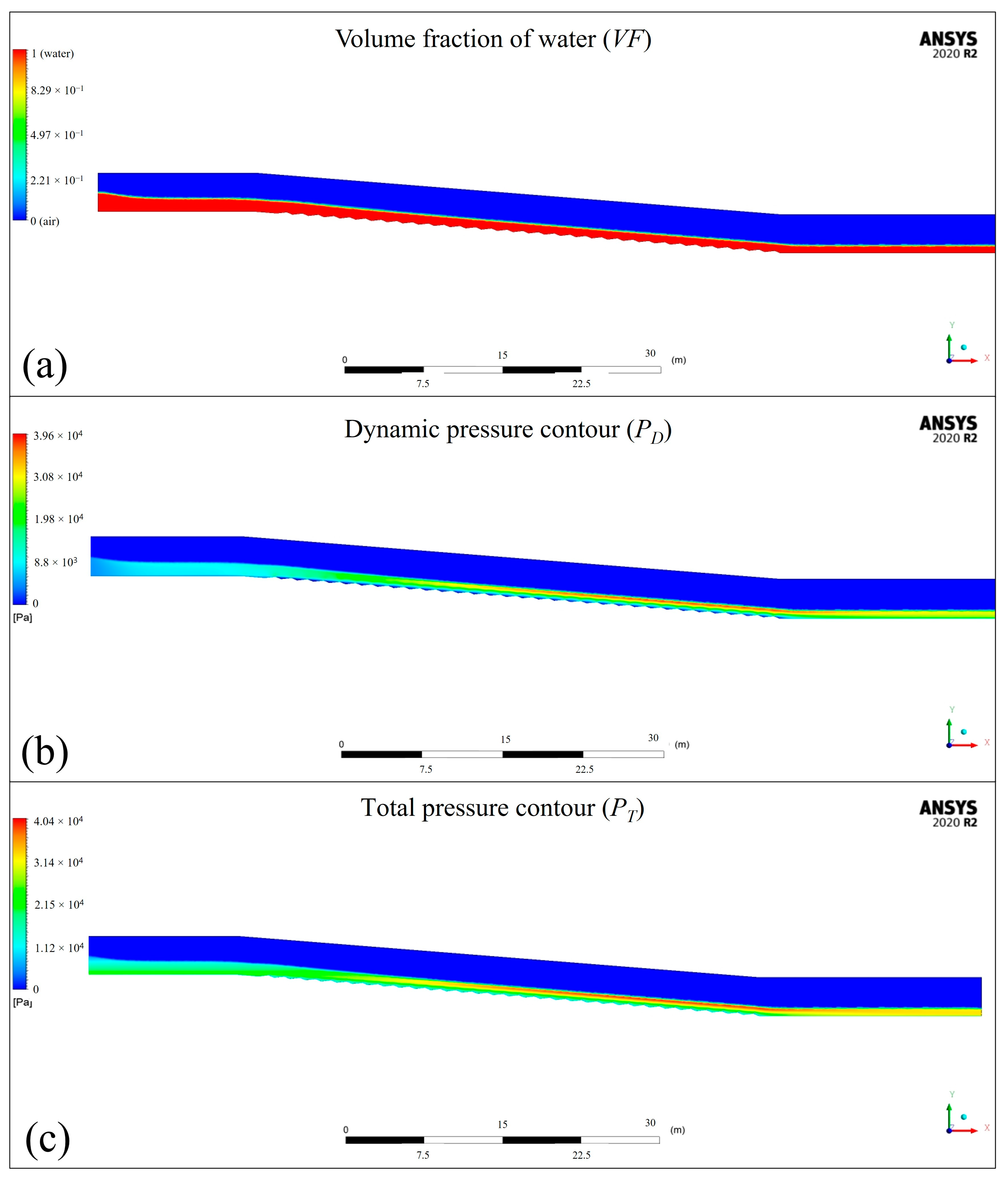
Figure 7 shows the software output, depicting the volume fraction of water (
VF), the contours of dynamic pressure (
PD) and total pressure (
PT) extracted directly from Ansys_Fluent.
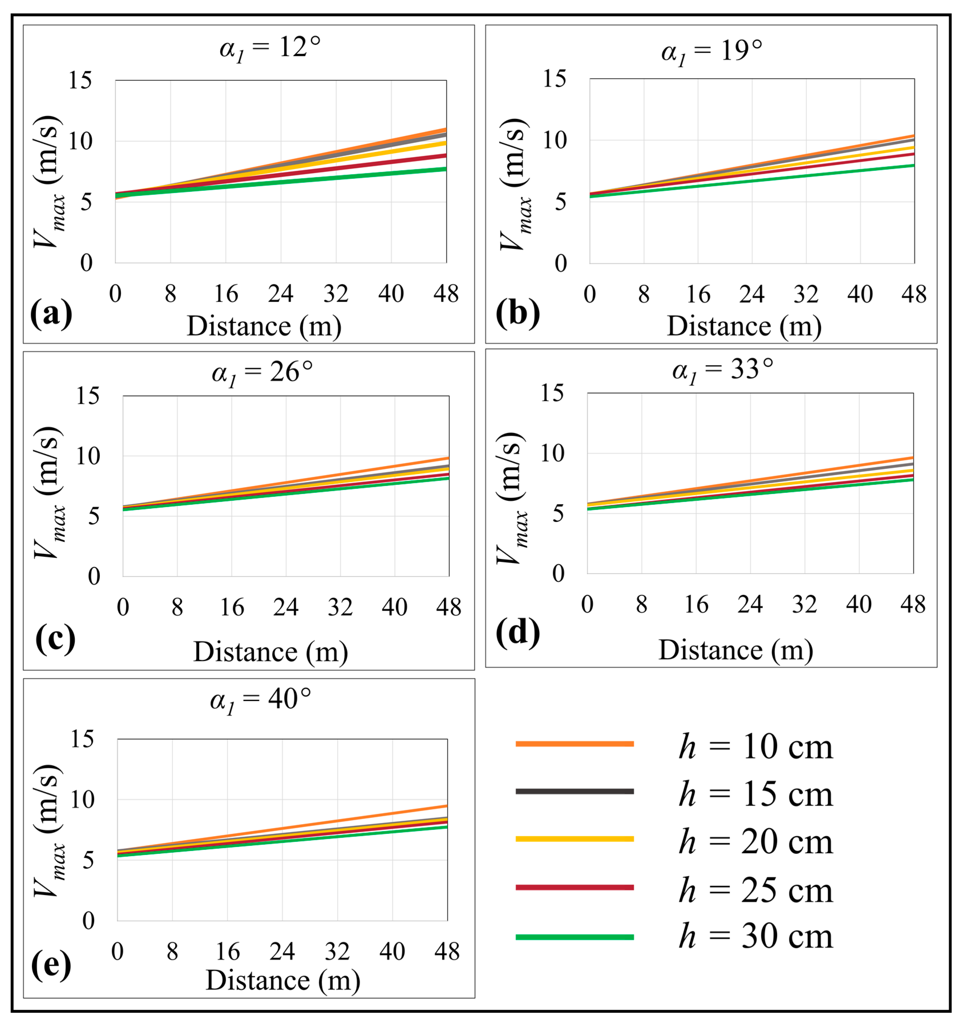
3.1. Effect of Irregularities on Velocity
Eleven vertical cross-sections were analyzed along the spillway to estimate the maximum velocity profile. Each section covered the channel bottom to the water’s surface, allowing us to calculate maximum velocity and water depth. Along the spillway, maximum velocity decreased as
α1 and height increased (
Figure 8). Moreover, the effect of height on flow velocity was greater than the effect of
α1. For instance, at a constant
α1 (
α1 = 12), maximum velocity decreased from approx. 11.5 m∙s
−1 at
h = 10 cm to approx. 8 m∙s
−1 at
h = 40 cm. At a constant height, however, velocity did not necessarily decrease as
α1 increased, the change often being minor and could be ignored. For instance, at a constant height (
h = 10 cm), the maximum velocity for
α1 = 12 was approx. 11.5 m∙s
−1 and for
α1 = 40, it was approx. 9 m∙s
−1. Flow velocity did not change significantly at a constant height (i.e,
h = 30 cm) as
α1 increased. At greater heights (
h),
α1 variations did not affect maximum velocity, and the height of the irregularity had a greater impact.
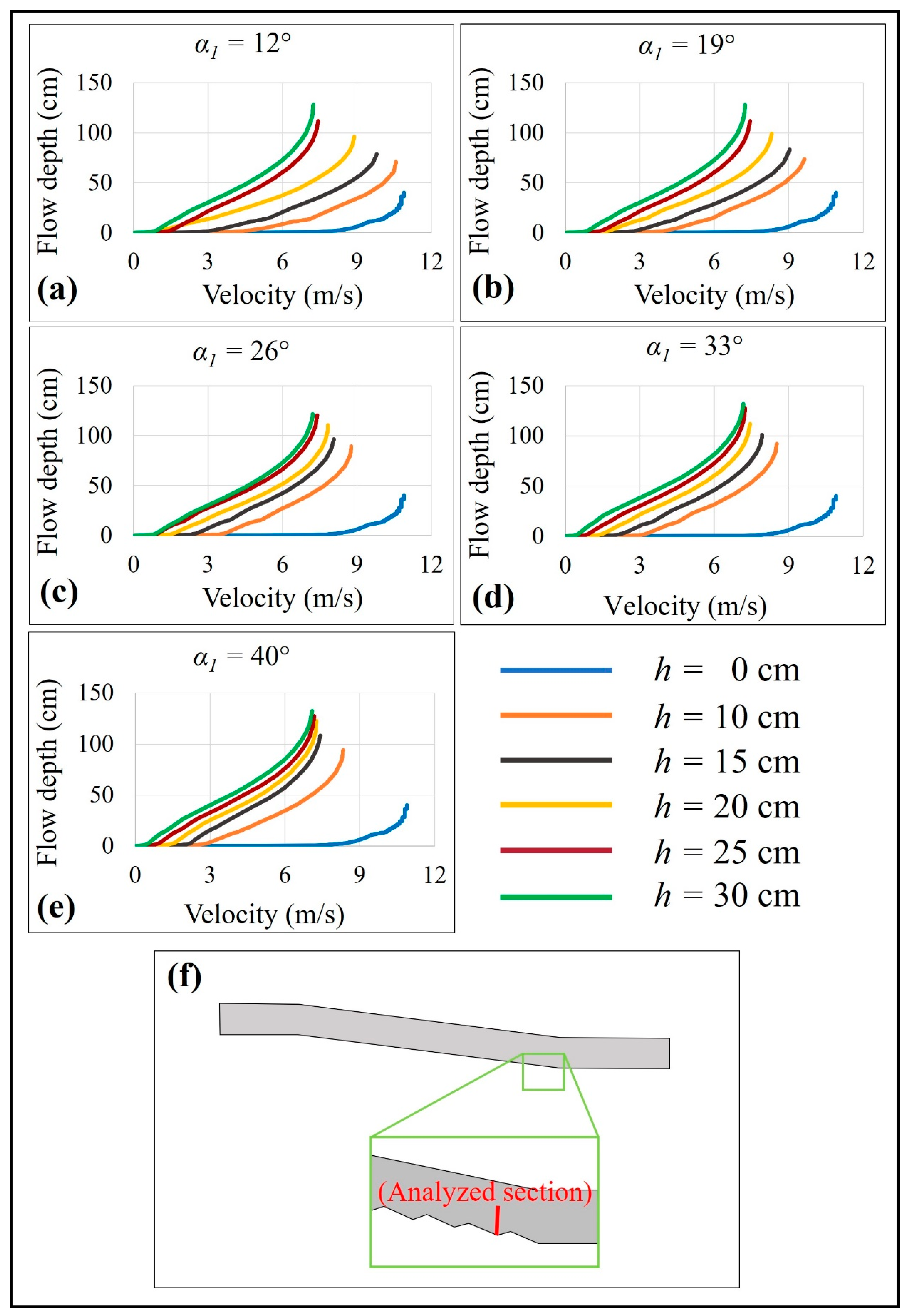
When velocity was evaluated as a function of flow depth at various irregularity heights (for the final irregularity along the channel), it was observed that a greater irregularity height, at a constant irregularity angle, caused water depth to increase, and the maximum velocity was also higher (
Figure 9).
3.2. Effect of Irregularities on Total Pressure (PT)
In hydraulic engineering, total pressure is the sum of static and dynamic pressures. The relationship between total, static (
PS), and dynamic (
PD) pressures are described in Equations (12)–(14), respectively.
where
ρ is the density of water,
g is the gravitational acceleration,
d is the water depth, and
v is the local flow velocity.
Total pressure in the first section was derived directly from the ANSYS-Fluent results, which produced a total pressure profile at the water–rock interface (channel bottom). When static pressure was at its maximum, dynamic pressure was at its minimum (Equation (15)).
When calculating the total pressure, both the maximum static and maximum dynamic pressure were considered (Equation (16)).
where
PT,max represents maximum total pressure,
PS,channel bottom represents the static pressure at the channel bottom,
PD,channel bottom represents the dynamic pressure at the channel bottom, and
PD,water surface is the dynamic pressure at the water surface, where it is at its maximum.
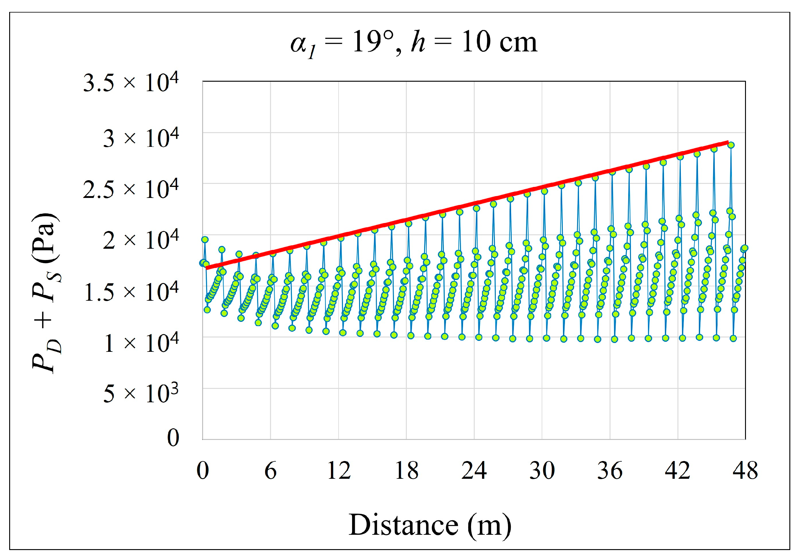
At the bottom of the channel, total pressure fluctuated along the spillway length (
Figure 10, for
h = 10 cm and
α1 = 19°). To analyze these fluctuations, the most representative and appropriate lines, which represented the upper bound of each graph (e.g., red line of
Figure 10), for each configuration were selected. These lines were then grouped into a single chart (
Figure 11).
Flow velocity increased, and water depth decreased moving downstream; thus, dynamic pressure, which has a direct relationship with flow velocity, trended upward, whereas static pressure, which has a direct relationship with water depth, trended downward along the channel. Overall, total pressure increased toward the downstream end of the profile. According to hydraulic engineering theory, however, flow velocity at the channel bottom is zero; thus, the dynamic pressure should also be zero. Total pressure at the channel bottom should be a function of static pressure, which also trends downward along the profile. The apparent contradiction of an increasing total pressure along the channel bottom and the greater role of dynamic pressure arose as the ANSYS-Fluent software records dynamic pressures at the mesh cell center. The value shown along the wall appears to be an extrapolation that does not necessarily equal zero.
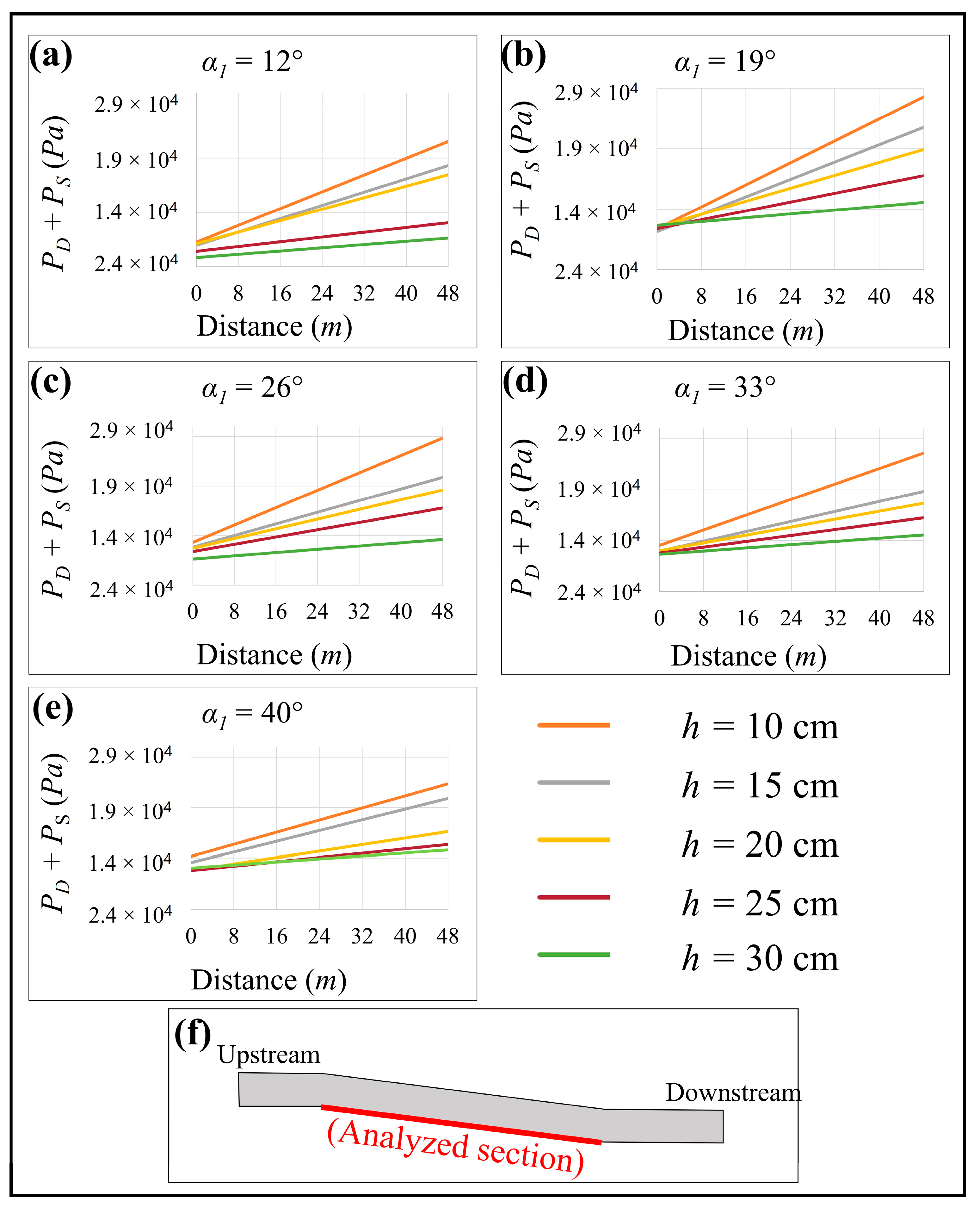
It was observed that total pressure decreased as
α1 and h increased (
Figure 11). For example, at a constant
α1 = 12°, the total pressure of flowing water at the channel bottom dropped with a higher
h, from approx. 25 Pa at
h = 10 cm to approx. 17 Pa at
h = 40 cm. At a constant
h, however, total pressure did not necessarily decrease as
α1 increased; often these changes were negligible and could be ignored. At greater heights (
h), altering
α1 produced little effect on total pressure, whereas altering the height of the irregularity had a marked effect. The total pressure difference at the zero point occurred because the zero point on the X-axis (distance) did not match the model’s zero point (see
Figure 11f). The analysis began 15 m from the model’s inlet; thus, the effect of irregularity height could already be observed, causing the initial pressure difference in the graphs.
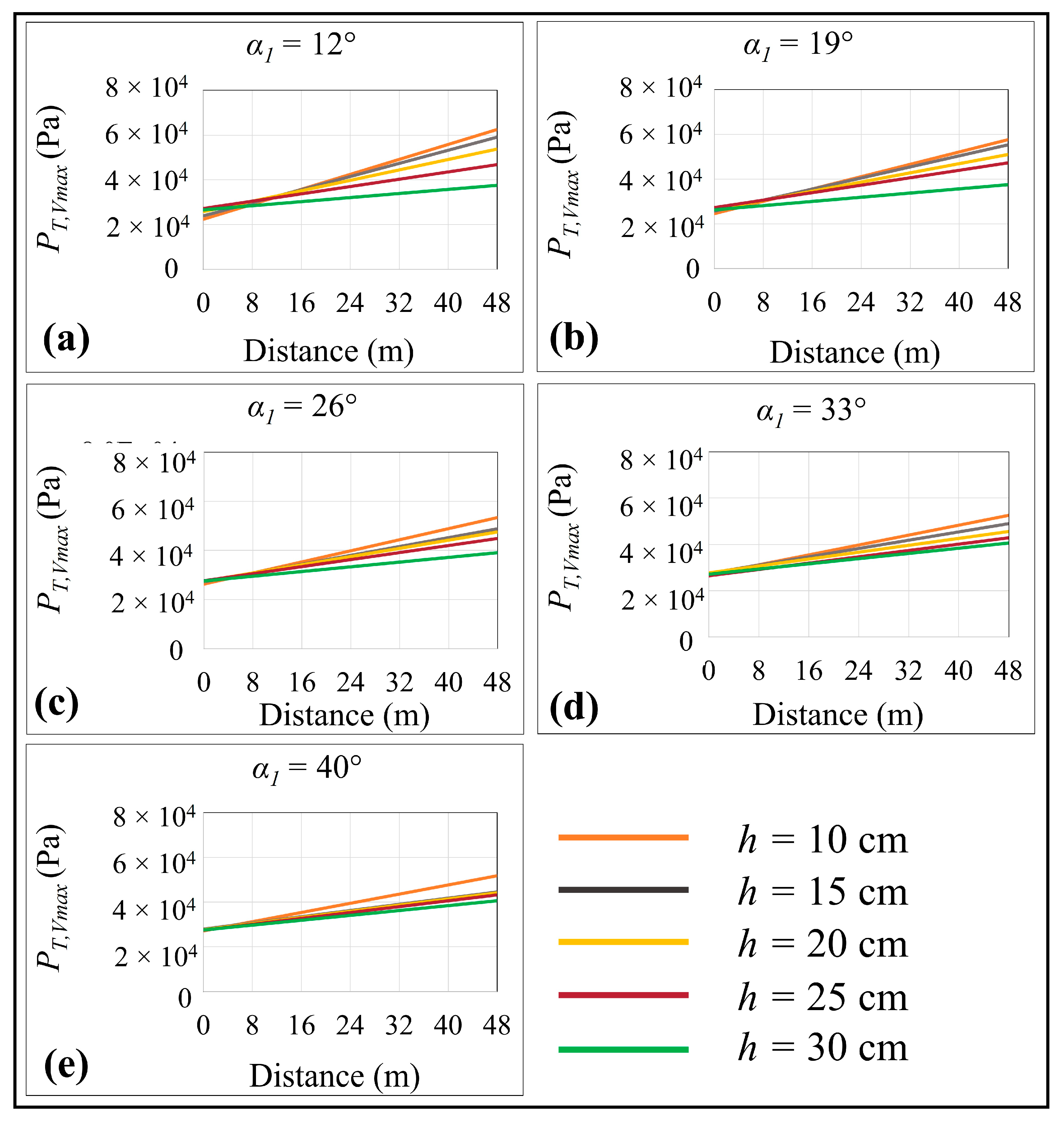
The total pressure was calculated using Equation (16). Since dynamic pressure is determined using the maximum velocity, the total pressure reached its maximum at the highest velocities (
Figure 12). Consequently, both dynamic and static pressures along the channel bottom were also at their maximum. Additionally, it was observed that the total pressure increased by 2.5–3 times compared to the pressure along the channel bottom. Total pressure also decreased as
α1 and
h increased (
Figure 12). At greater heights (
h),
α1 changes had minimal effect on the total pressure, whereas changes to irregularity height did produce a large effect.
3.3. Effect of Irregularities on Shear Stress
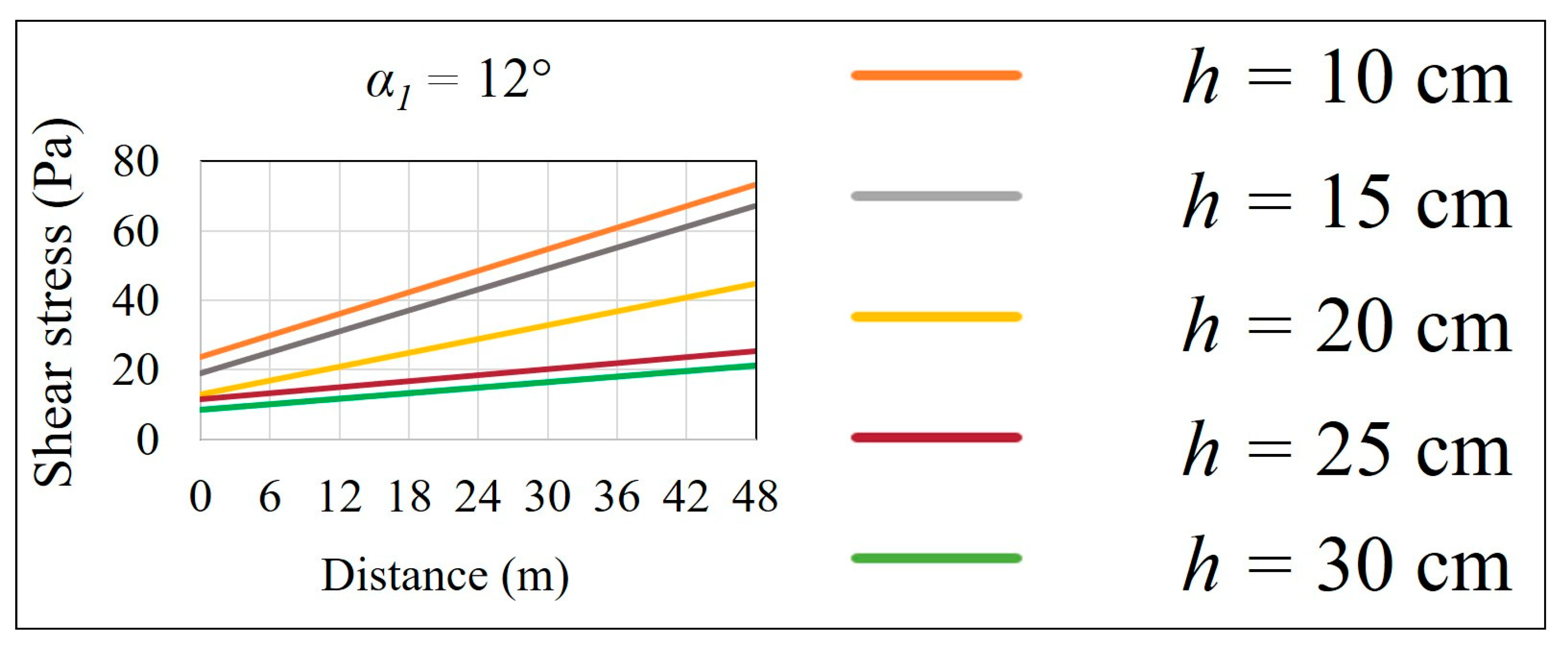
Shear stress at the water–rock interface was also investigated.
Figure 13 shows the surface shear stress on the rock surface for an irregularity angle of
α1 = 12. Shear stress on the rock surface was negligible relative to the total, static, and dynamic pressures. Nonetheless, as irregularity height (
h) increased, shear stress along the wall decreased; however, these values were so small that they could be ignored.
3.4. Effect of Irregularities on the Energy Gradient
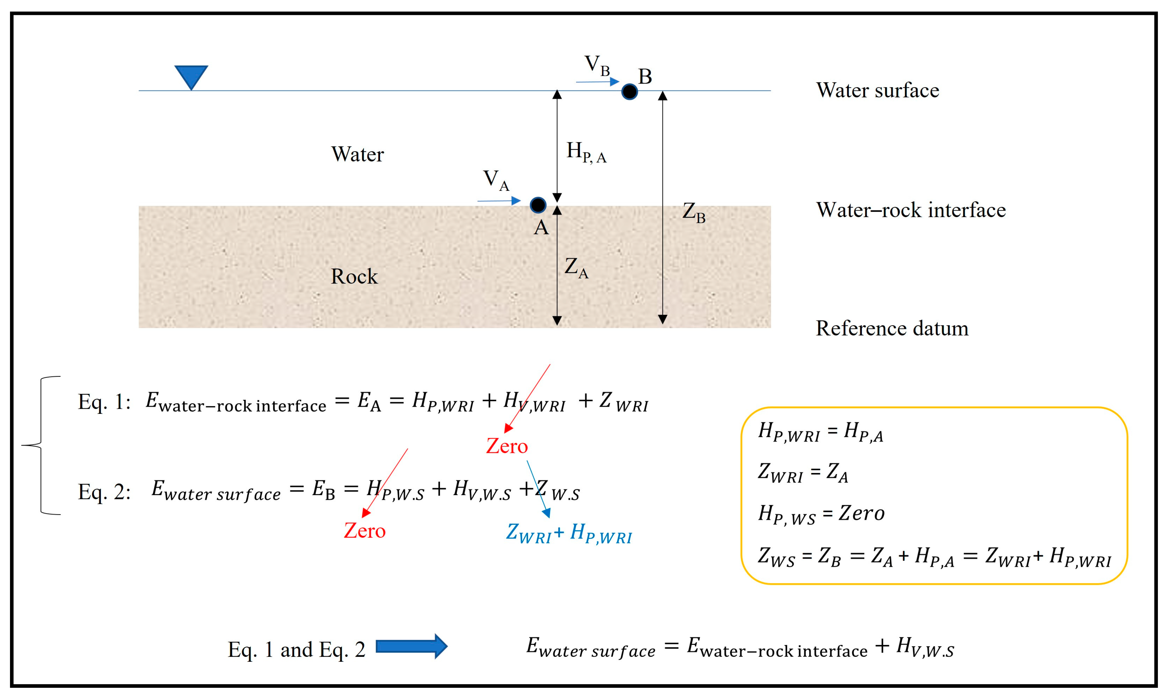
In the preceding section, the sum of pressure and velocity heads, i.e., dynamic and static pressure, for two distinct states of dynamic pressure, namely (1) at the rock mass surface and (2) at the water surface, was described. Here, the energy at (1) the water surface and (2) the channel bottom was analyzed.
The relevant energy was computed using Equations (17) and (18), with velocity head determined directly from the flow velocity, and pressure head equal to water depth. The elevation of a point was its distance from the datum.
where
represents the energy at the channel bottom,
and
are the pressure head and velocity head, respectively, at the channel bottom.
is the elevation of the channel bottom,
is the energy at the water surface,
and
represent, respectively, the pressure head and velocity head at the water surface,
is the elevation of the water surface from the datum, and
. These parameters are mesured in meters.
For calculating the energy at the rock mass surface, the velocity head was at a minimum and the pressure head at a maximum. In contrast, at the water surface, the velocity head was at a maximum, and the pressure head was zero. The difference between the energy at the water surface and the energy at the channel bottom (
) was the velocity head or dynamic pressure.
Figure 14 describes the methodology to calculate energy at the water–rock interface and water surface.
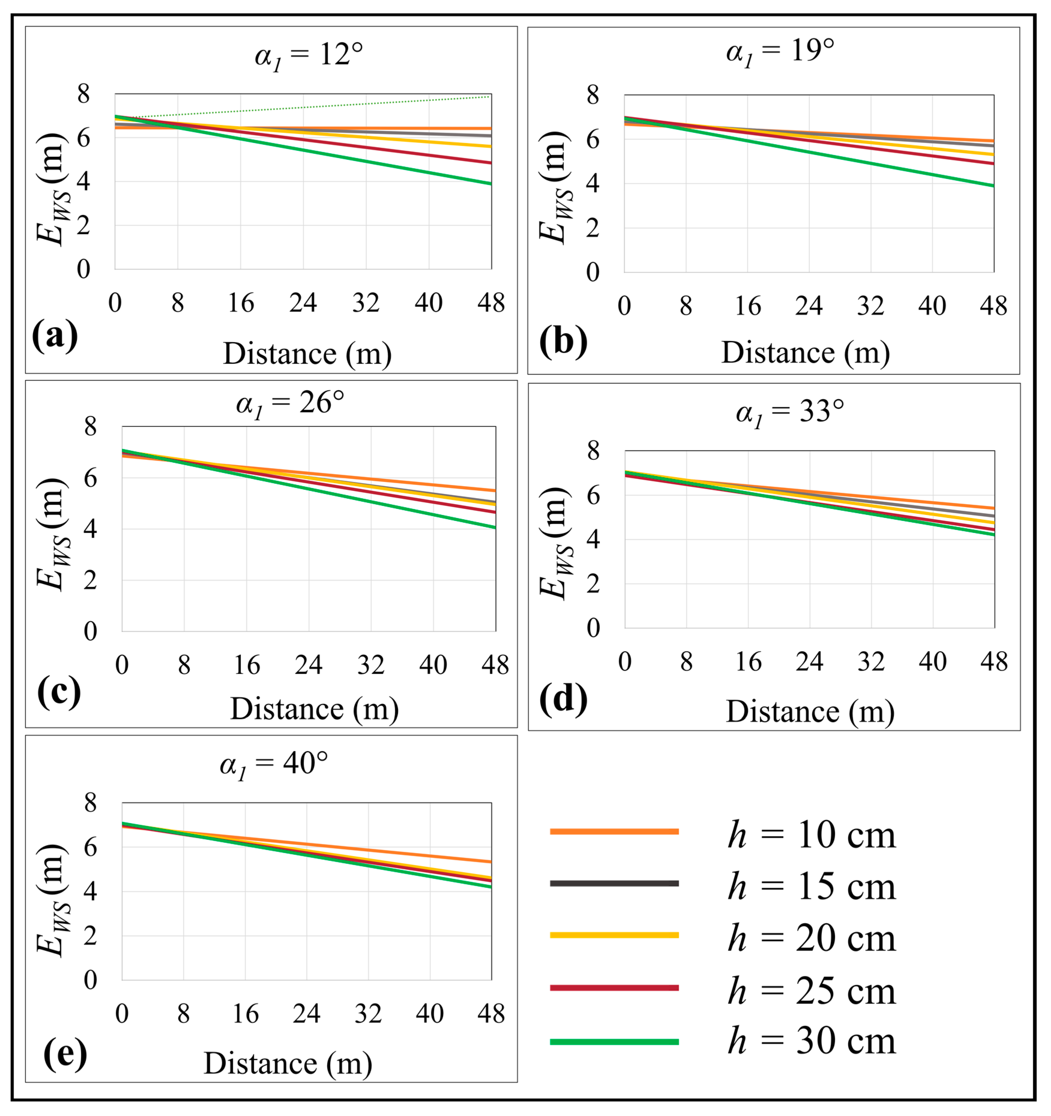
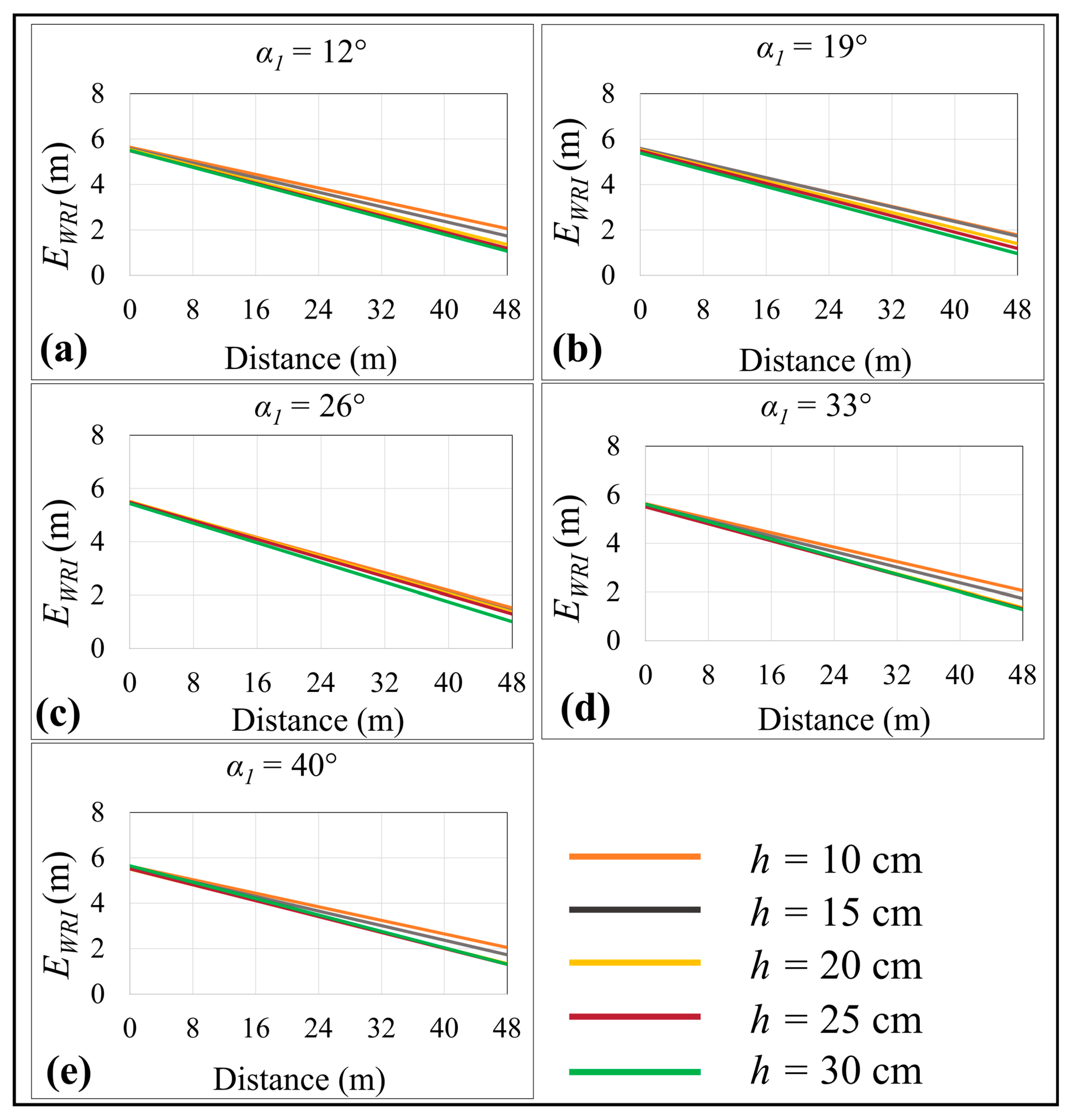
The energy of water at the water–rock interface and water surface for the entire analyzed area was then calculated. Energy gradients and differences in energy along the profile were also depicted (
Figure 15). Energy decreased upstream to downstream, with 70% of the energy lost along the profile. When the angle was held constant, as h increased, a greater amount of energy was lost. Less energy was lost when h decreased. At a constant h, however, energy loss was not necessarily greater as α
1 increased.
Energy at the water surface (State 1) where energy relates to elevation and velocity head (at their maximum) and the pressure head are at their minimum. Energy increased along the profile relative to the energy at the water–rock interface (State 2). This energy increase was around 30% upstream and 2.5–3.5× times downstream relative to the energy at water–rock interface.
Differences in the energy state at the water–rock interface (
Figure 15) and the water surface (
Figure 16) related to the flow velocity and dynamic pressure.
Energy loss at the water–rock interface (State 1) was greater than at the water surface (State 2) because:
In the first state, the velocity differential between upstream and downstream was close to zero; thus, the slope of the flow–distance relationship was zero;
In the second state, the difference in velocity between the upstream and downstream was not zero, and flow velocity–distance relationship sloped upward.
Because the sum of Z and HP was the same for both states, the negative relationship between the energy and distance decreased as the slope of the velocity increased for the second state, i.e., a greater velocity increased the amount of energy and decreased energy loss.
4. Discussion
Our study demonstrated the successful use of ANSYS-Fluent software and 2D steady-state simulations using computational fluid dynamics to determine the effect of unlined spillway surface irregularities (height and angle) on hydraulic parameters. The study focused on how changes to irregularity height and angle affected flow velocity, dynamic pressure, static pressure, total pressure, shear stress, velocity head, pressure head, elevation, energy, and energy loss. The findings revealed that:
- (1)
Irregularities affected hydraulic parameters, despite existing approaches for determining hydraulic erosive parameters not considering these irregularities.
- (2)
Velocity at a constant height did not continually decrease as α1 increased, and these changes were often negligible.
- (3)
Changes in irregularity angle had a minimal effect on maximum flow velocity at greater heights; however, altering irregularity height had a marked effect.
- (4)
Holding the irregularity angle constant, total pressure along the channel bottom decreased as h increased. At a constant h, however, total pressure did not consistently decrease as α1 increased; these latter changes were typically negligible. At greater heights, changes in angle had a minimal impact on total pressure; however, altering irregularity height had a marked effect.
- (5)
Total pressure, using maximum dynamic pressure to determine the total pressure, increased 2.5–3× relative pressure along the channel bottom.
- (6)
Along the water–rock interface, 70% of the energy was lost along the profile.
- (7)
Energy at the water–rock interface increased by approx. 30% upstream and 250%–350% downstream.
- (8)
Increased flow velocity increased energy and decreased energy loss.
It should be noted that the 2D nature of this research represented a limitation. Additionally, the simulations were steady-state and not time-dependent (transient). Furthermore, the effect of geometric characteristics of the unlined spillway, i.e., overall spillway profile and length, was not considered in this study. Future research should address these limitations to provide a more comprehensive understanding of the subject.


