1. Introduction
Although climate change adaptation and response are pre-empted worldwide, disasters caused by climate change continue to occur. In 2022, in Pakistan, one-third of the country was flooded with heavy rains for three months starting on 14 June, and the number of victims was estimated to be 33 million. In Seoul, the capital of the Republic of Korea and a world-class metropolis, heavy rains for two days caused many casualties, and the vehicle flooding damage alone was estimated to be USD 98.8 million. In the Southwest of the United States, which has been experiencing the worst drought and heat wave in 1200 years, at least 25 people have died, and the Las Vegas desert turned into a flooded area due to a heavy rain. In 2021, 242 people died due to heavy rain in Benelux, Germany, and property damage incurred costs of more than EUR 10 billion. Disasters caused by climate change are occurring not only in developed countries but also around the world. Flooding in a large city is used as a measure of the level of the city’s social system because the damage per unit area is higher than that of the general area due to high-density development and artificial space in the underground space. Flood inundation modeling in large cities such as Seoul is affected by artificial factors including land use and pipe network systems, so it is important to estimate the parameters associated with these factors to obtain accurate analysis results.
Many studies have been conducted around the world to analyze the parameter uncertainty of the rainfall-runoff model and to optimize it via 1D and 2D urban flooding analysis. Duan [
1] developed the SCE (Shuffled Complex Evolution)–UA (University of Arizona) technique to solve the parameter optimization problem of the rainfall–runoff model. Hope et al. [
2] applied the GLUE (Generalized Likelihood Uncertainty Estimation) to the Hydrologic Simulation Program Fortran (HSPF) for modeling optimization according to the number of parameters, and Skahill and Doherty [
3] applied the PEST (Parameter ESTimation) technique to optimize runoff. Bahremand et al. [
4] conducted a study on automatic calibration, sensitivity ranking, and optimization using PEST in a grid–type distributed hydrological model called WetSpa (Water and Energy Transfer between Soil, Plants and Atmosphere). Kim et al. [
5] conducted a study on the optimization of urban runoff parameters using a 2D flooded area by generating a scenario using eight parameters in the Bisan-dong watershed of Daegu, Korea.
With the development of computer technology, many studies have been conducted on 1D–1D or 1D–2D combined models that can simultaneously analyze the pipe network flow and perform flood inundation analysis. Mark et al. [
6] and Leandro et al. [
7] presented the strengths and weaknesses of each model in urban inundation analysis via a comparison of 1D–1D and 1D–2D coupled models. Turner et al. [
8], Mason et al. [
9], and Leitão et al. [
10] conducted studies using LiDAR (Light Detection and Ranging) and DSM (Digital Surface Model) to increase the accuracy of inundation analysis around roads and buildings. In addition, Son et al. [
11] conducted a study on flood analysis considering underground space in urban areas, and Ha [
12] performed a coupled analysis of 1D–2D models for urban flood optimization simulation. Andreja et al. [
13] analyzed 1D–2D linkages using global optimization techniques for the Huai River in China, and Georgios et al. [
14] conducted a coupled analysis using the HEC–RAS 1D–2D model for flash floods in Attica Mandra, Greece, in November 2017.
Optimization studies have been conducted using automatic calibration techniques for parameter sensitivity and uncertainty analysis, including the above-mentioned studies. However, in most studies, the observed data used for model calibration were not the observed water level of the pipeline in the study area, but the observation level of the natural river or the discharge of the drainage pumping station. In addition, most of the optimization of 1D–2D linkage models has been conducted in studies based on the accuracy of terrain data [
8,
9,
10], and Fraga et al. [
15] performed sensitivity analysis and optimization for six parameters using GLUE in the 1D–2D dual urban drainage model, but this was applied only to one small drainage area (4.9 ha). The optimization of major parameters is important for the accurate evaluation of the urban drainage capacity and overflow of the urban pipe network system. In particular, the minimum pipe diameter reflected in the model affects efficiency in terms of the number of parameters, the time required for input data construction, and calculation time. Additionally, it impacts the positioning of the overflow manhole and the flow calculation within the pipe.
Therefore, in this study, the sub-catchments were classified according to the minimum pipe diameter for the study basin, and then parameter estimation and runoff analysis were performed. In addition, the effect of optimization considering the parameter sensitivity on the accuracy of runoff was analyzed using the water level of the pipe in the study area. In addition, the accuracy was compared and analyzed according to the minimum pipe diameter in the 1D–2D urban flooding linkage analysis in order to present the standard appropriate pipe diameter size, and the effect of 1D urban runoff parameter optimization on the linkage simulation was analyzed in order to improve the accuracy.
2. Research Method
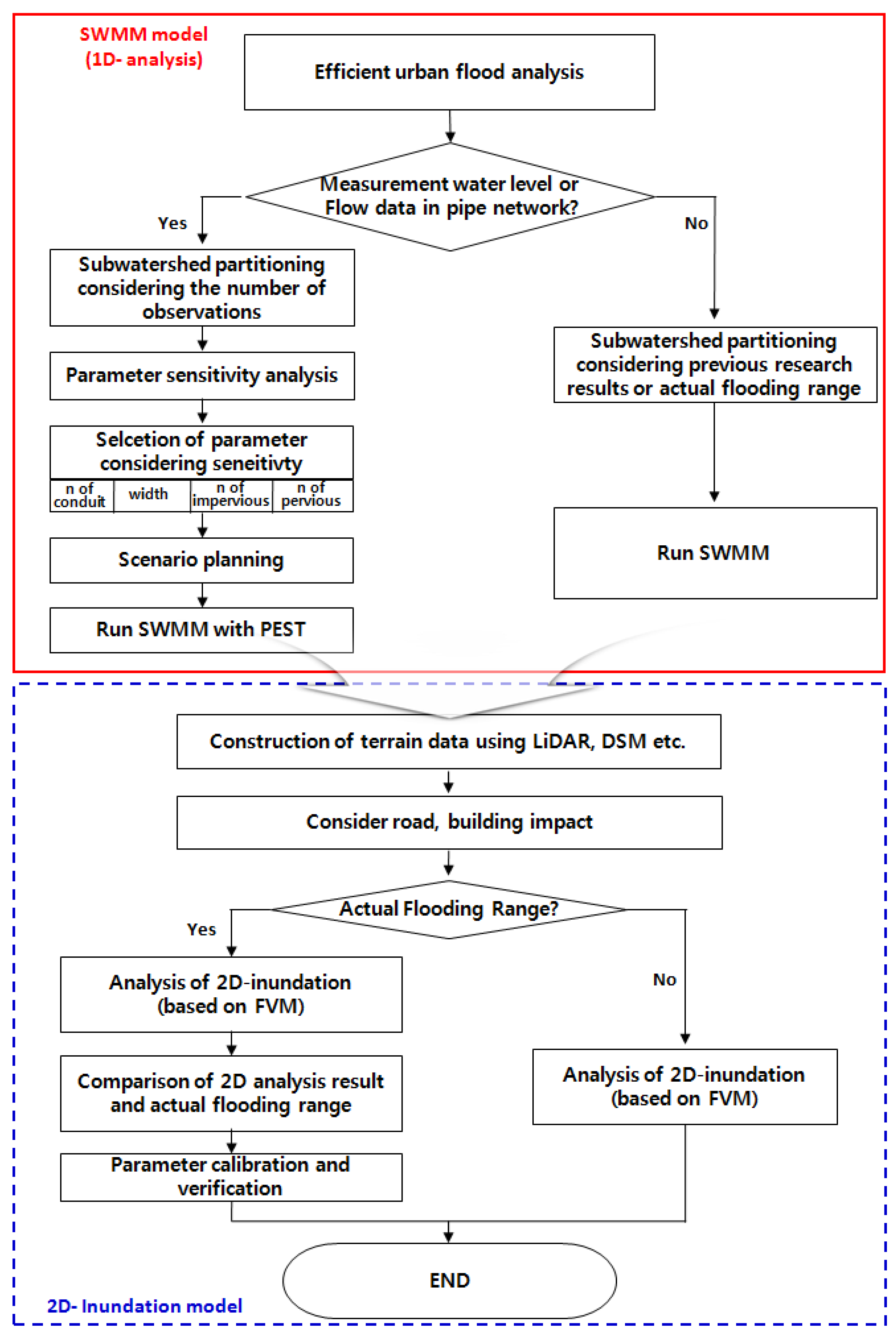
The main causes of urban flooding are the lack of capacity in sewage pipes and the difficulty of drainage due to rising river levels. It is important to calculate the minimum diameter and proper parameter values of the pipe applied to the overflow location and overflow amount. In actual urban runoff analysis, sub-catchments are divided as extensively as possible to account for a substantial number of drainage pipes. As the number of sub-catchments increases, the parameters for each sub-catchment are calculated separately, so the number of parameters increases proportionally with the number of sub-catchments. Therefore, in this study, scenarios were created by varying the number and diameter of urban sewage pipes for the analysis of the urban sewer network as shown in
Figure 1.
The appropriate parameters of the SWMM were determined by applying PEST; the overflow in manholes and the flooded area in the 2D flood analysis were calculated for each scenario and the accuracy was compared. This study proposes an appropriate sewage pipe diameter to be considered in 1D–2D urban flood analysis and aims to improve the accuracy and efficiency through the parameter optimization of the applied model.
Parameter ESTimation (PEST)
Parametric optimization is the process of finding a combination of parameters that maximizes or minimizes the function value of the objective function. Optimization methods include empirical techniques, mathematical techniques, and search methods that are used to optimize objective functions [
16]. PEST is based on the Gauss–Marquardt–Levenberg (GML) algorithm, which is one of the nonlinear regression methods [
17]. Advanced techniques that are used for multi-dimensional parameter estimation, such as pilot points and normalization, are supported as options, and the Global Optimization technique can estimate parameters with a short calculation time compared to SCE–UA. In addition, if the conditions for controlling the execution file of the model from the outside are satisfied, it is possible to link them without modifying the internal code, regardless of the type of model to be applied.
As shown in Equation (1), the relationship between the parameters and calculated values for the nonlinear model can be expressed as a function K, which is an n-dimensional parameter space corresponding to the m-dimensional measured value parameter space. The relational function K continuously interacts while considering all model parameters. Assume that the nonlinear model (function K) generated by the set of parameters corresponding to the vector b is equal to c.
Here, a series of observation results, c, corresponding to a parameter vector, b, that is slightly different from,
is generated, and the approximate value according to the proximity between
and
is calculated using Taylor’s theorem, as follows:
where, J = Jacobia matrix of K; this is a matrix composed of m columns (one for each measured value) and n elements, and in each row there is a derivative model of a specific measured value associated with each parameter. Equation (2) is a linearization of Equation (1).
Now, to deduce the parameters for the model that presents the nearest calculated value within the least square root of the measured value,
, the objective function defined in Equation (3) is determined as a parameter for the minimum value.
In , (i-th error) represents the difference between the modeling result and the actual value for the i-th observation.
And, the parameter upgrade vector can be expressed as Equation (4).
This is described as Equation (5) of the parametric covariance matrix.
Since Equation (2) is a linear equation, Equation (4) also has no error. In other words, the vector, b, is defined by adding the parameter upgrade vector, u, in Equation (4). The current parameter value is not guaranteed to allow the objective function to reach its minimum. Therefore, the new set of parameters included in should be used as a starting point to determine the next parameter upgrade vector, which will finally reach the optimization of the objective function .
Finding the whole minimum of the objective function in nonlinear optimization problems is a difficult problem. The proper selection of initial parameters can reduce the number of iterations required to minimize the objective function. Also, incorporating prior information into the objective function can often change the structure in the parameter space (weighted according to what applies to prior information) and make it easier to find local minima. This enhances the optimization stability and reduces the number of iterations required to determine the optimal set of parameters.
Figure 2 shows the iterative change process of the initial parameter values for global objective function optimization.
3. Study Area and Parameter Sensitivity Analysis
3.1. Study Area
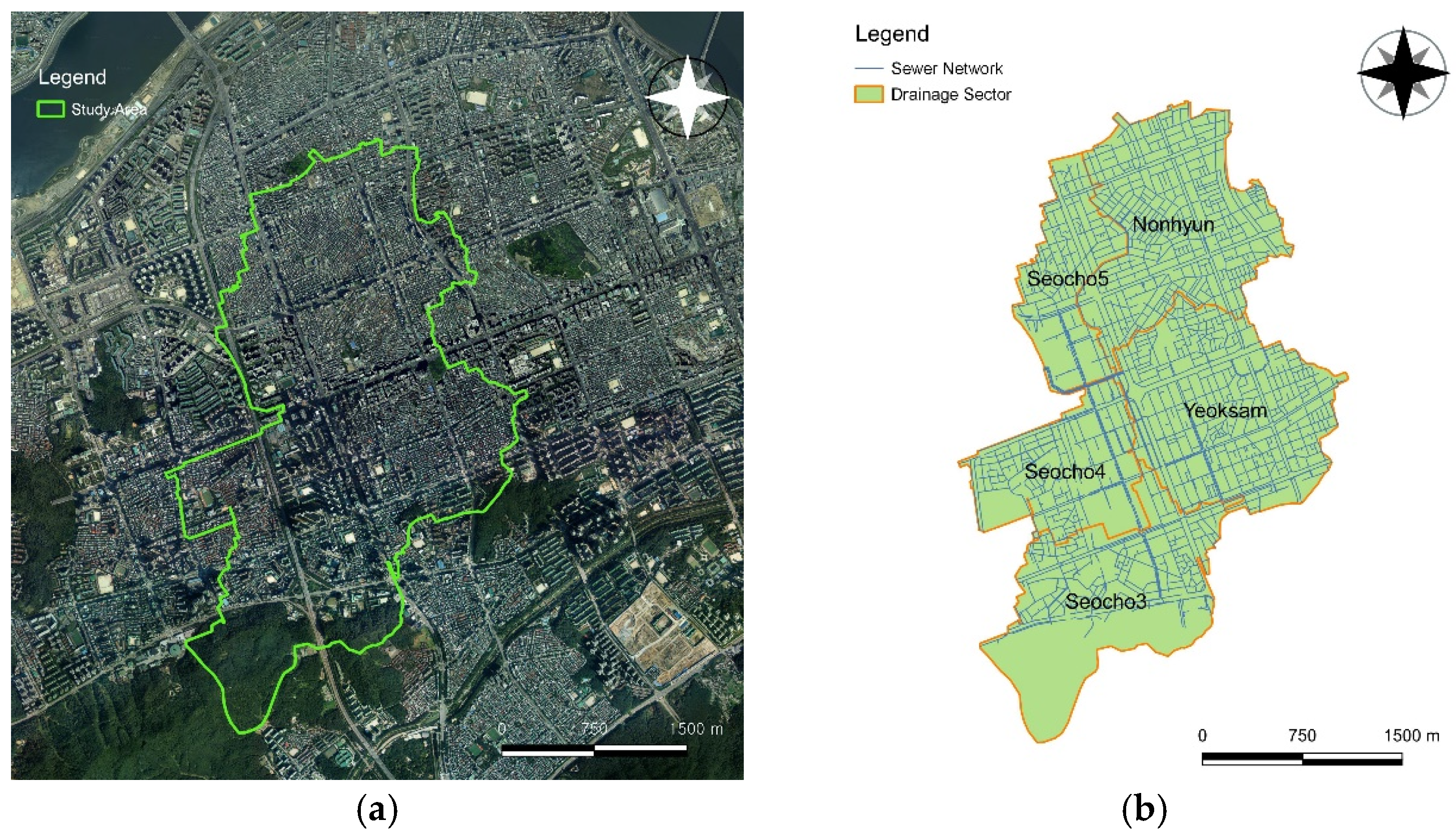
The study area of this study was the Banpo drainage area, which flows into Banpocheon through 239 drainage basins in 16 drainage districts in Seoul, Korea, and the Nonhyeon, Yeoksam, and Seocho 3, 4, and 5 drainage basins where actual inundation damage occurred in 2013 (
Figure 3). Five drainage basins are administratively located in Seocho-gu and Gangnam-gu, and the total area is 739.21 ha. Most of the drainage passes through Gangnam Station and flows into the Banpocheon stream, which passes from the intersection behind the former New York bakery to the Seocho Elementary School. When the water level of Banpocheon rose due to localized heavy rains and drainage became difficult, flooding damage was caused to the Gangnam Station area and the Yeoksam and Seocho drainage basins. This is an urbanized region in which residential and commercial areas are concentrated, and the impervious rate is high at over 90%. As a result, the runoff increases, and the time to reach the peak runoff is short, so the possibility of inundation is high. The satellite image and drainage network map of the study catchment are shown in
Figure 3a,b, respectively, and the total number of manholes and storm sewers is 4125 and 5853, respectively. The catchment and pipe network properties for each drainage basin are shown in
Table 1. As shown in
Table 2, two water level gauges were used for the manhole water level observation data. Since 2013, when the water level gauge was installed in Seoul, flood damage due to heavy rains or typhoons has not occurred very often, so parameter optimization simulations were performed using PEST for the rainfall on 22 July 2013, when flood damage was reported. The parameter verification for the one-dimensional pipe network runoff was performed for the rainfall event between 2013 and 2014, and 2D flood analysis verification was performed for the rainfall event on 21 September 2010, when significant flood damage actually occurred.
3.2. Building Parameters for Sub-Catchments
Yoon and Yoon [
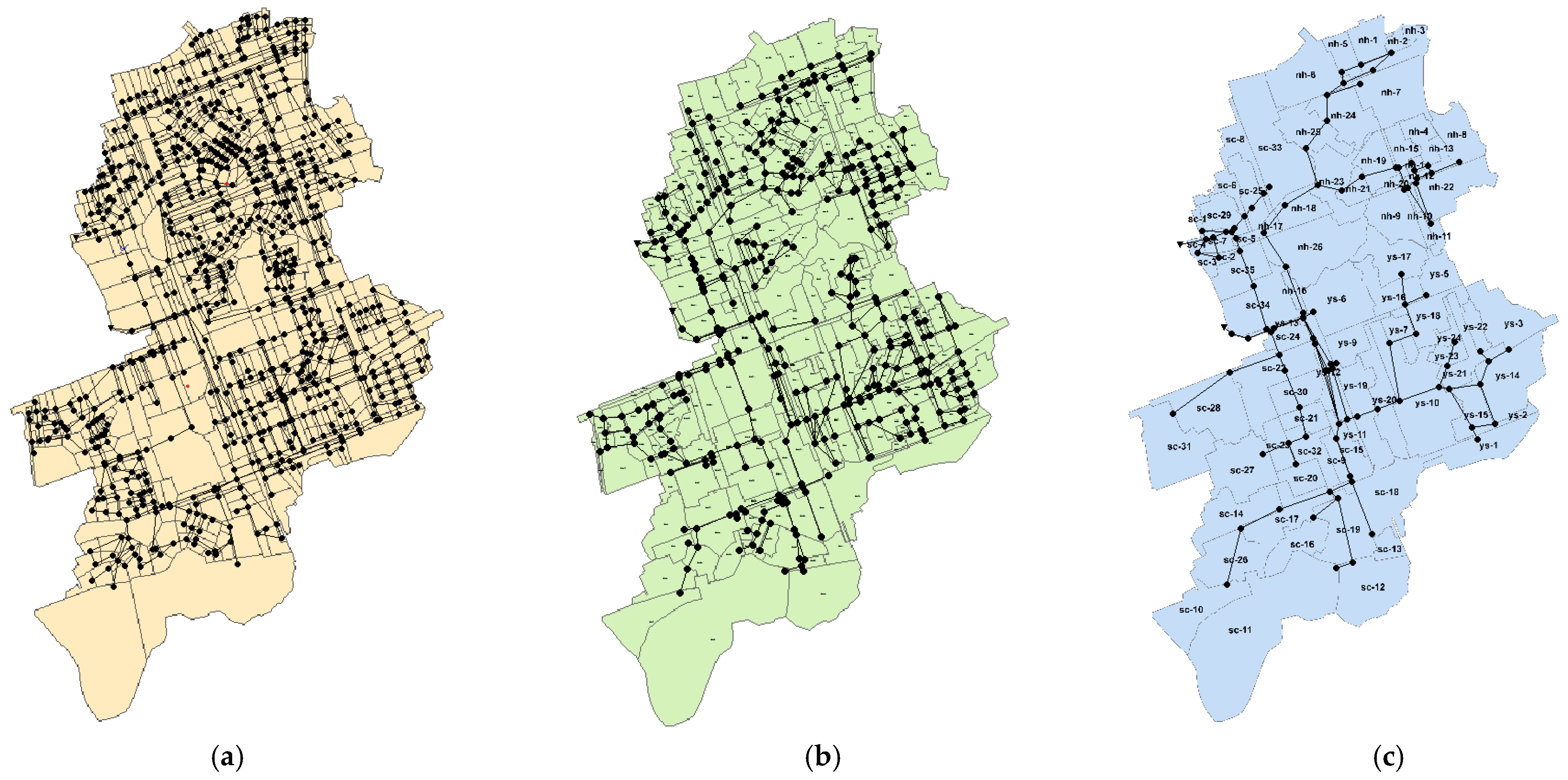
19] compared the runoff accuracy according to the number of sub-catchments and showed that the uncertainty increased when the sub-catchment was divided into several regions, and that the runoff error was larger than that of a single watershed. In highly urbanized areas, urban drainage systems and sub-catchments need to be realistically considered and analyzed. If the number of sub-catchments is simplified too much, the urban drainage system may be distorted. Therefore, the study catchment was divided into three cases (
Figure 4), and the difference between the water level of the urban drainage system and the actual flood pattern was compared according to the number of sub-catchments in the urbanized drainage basin.
First, by using pipelines of 450 mm or more and a 94% application rate for all of the conduits, topographical data were established; the sub-catchments were composed of 772 and 1062 pipelines, which are shown in
Figure 4a. Second, by constructing topographical data and a 63% application rate for all of the conduits using pipelines of 600 mm or more, the sub-region consisted of 310 pipelines and 482 pipelines, which are shown in
Figure 4b. Lastly, the construction of topographical data using pipelines of 1200 mm or more and consisting only of mainlines comprised 83 sub-regions and 120 pipelines using a 15.9% application rate for all of the conduits, as shown in
Figure 4c.
For the sub-catchment data, the factors for each basin and the average slope of each basin were calculated using the LiDAR of Seoul Metropolitan City, and the impervious rate was calculated using the 2015 Seoul metropolitan biotope map (
http://nationalatlas.ngii.go.kr, accessed on 13 October 2022). The slope, length, and specifications of the pipes were calculated using data from the national sewage information system (
https://www.hasudoinfo.or.kr, accessed on 13 October 2022).
3.3. Sensitivity Analysis
In this study, four parameters were determined when considering the results of previous studies related to parameters. Among the previous studies, Joo and Park [
20] quantified uncertainty and prioritized the parameters using a sensitivity analysis because the amount of runoff calculated via the simulation of the rainfall–runoff model affects its reliability. Chung et al. [
21] quantified the degree of uncertainty of six parameters using the uncertainty quantification index and analyzed the size of each parameter’s uncertainty. It was found that the roughness coefficients in conduits, impervious areas and pervious areas have large uncertainties. First of all, a pipe with a diameter of 1200 mm or more was used to analyze the sensitivity of the study area for scenario construction. The selected parameters were the sub-catchment width, the roughness coefficients of pervious and impervious basins, and the pipe roughness coefficient. The selected parameters and allowable ranges for application are shown in
Table 3. For Manning’s roughness coefficient, the range suggested by Mays [
22] was selected. The sub-catchment width is different for each calculated sub-catchment, and it is difficult to uniformly apply the range. As for the range in the sub-catchment width, 80% to 180% of the calculated sub-catchment width proposed by Barco et al. [
23] in a study on optimization using the automatic calibration method of the SWMM model was applied to the Ballona Creek drainage basin, a large-scale urban catchment. For the four parameters selected above (
Table 3), sensitivity was analyzed using PEST, and the statistical accuracy was estimated by comparing the observed water levels. The parameter sensitivity in PEST is equal to Equation (6).
where,
is a Jacobian matrix and
is a “cofactor matrix”; in most instances, the latter will be a diagonal matrix whose elements comprise the squared observation weights.
The composite observation sensitivity of observation
is equal to Equation (7).
where, the composite sensitivity of observation j is the size of the j-th row of the Jacobian matrix multiplied by the weight associated with that observation. Then, this size is divided by the number of adjustable parameters.
The parameter sensitivity to water level is shown in
Table 4. The results were in the order of Manning’s roughness coefficient for conduits, the roughness coefficient of the impervious basin, the width of the basin, and the roughness coefficient of the permeable basin. Unlike the preceding study by Chung et al. [
21], this study found that the roughness coefficient of the pervious area was less sensitive than the basin width. This is because the study area is a highly urbanized area and the pervious area is small.
4. Scenario Creation and 1D–2D Inundation Analysis
4.1. Scenario Creation and Accuracy Comparison considering Sensitivity
Using the parameter sensitivity of each sub-catchment analyzed in
Section 3.3, scenarios were created using three topographical data and four parameters, and each scenario was evaluated using coupled 1D and 2D modeling. For optimal urban runoff analysis, scenarios were created, as shown in
Table 5, to compare differences in the accuracy according to the number of optimization parameters and the sensitivity. Scenarios 4 and 5 considered three parameters. Scenario 4 considered the three parameters with high sensitivity estimated in this study, and scenario 5 considered the three parameters with high sensitivity shown in Chung et al. [
21].
Root Mean Square Error (RMSE) and Relative Peak Error (RPE) were used employed for error analysis using Equations (8) and (9), respectively.
Table 5 shows the statistical analysis results for each scenario.
where,
is the observed water level,
is the simulated water level, N is the number of observed time series,
is the observed peak water level, and
is the simulated peak water level. When comparing the uncalibrated S1 with the scenario using the automatic calibration method, the RMSE decreased by up to 2.37 cm (S3–S6), and the RPE decreased by 22.04% (S2–S4) (
Table 5). When comparing S4, which considers only the parameters with high sensitivity, and S5 and S6, which consider the roughness coefficient of the pervious area with the lowest sensitivity, it was found that the accuracy of S4 is slightly higher. Also, S5 and S6, which included the roughness coefficient of the pervious area, took more calculation time than S4, which did not consider this parameter. A scenario considering the sensitivity of the study area, S4, was shown to be more efficient for real-time modeling, as it can provide flood forecasting and alerts with greater accuracy and a shorter computational time.
Table 5 shows the error analysis results compared to the measured water levels for each scenario.
4.2. Urban Runoff and 1D Drainage Network Analysis
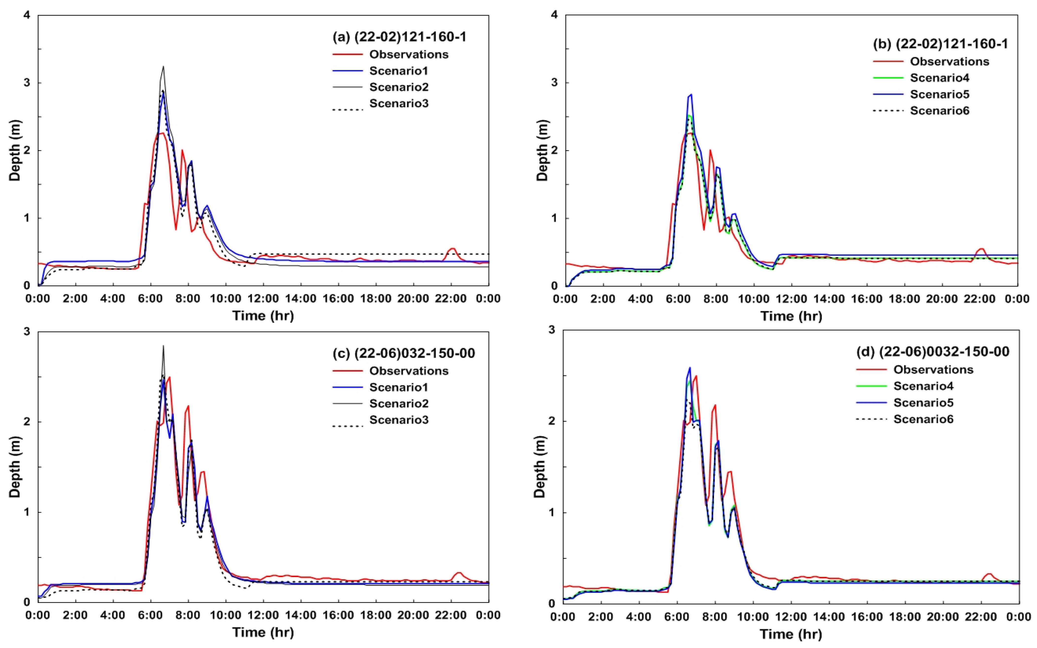
A comparison of the urban runoff analysis according to the scenario with the observed water level is shown in
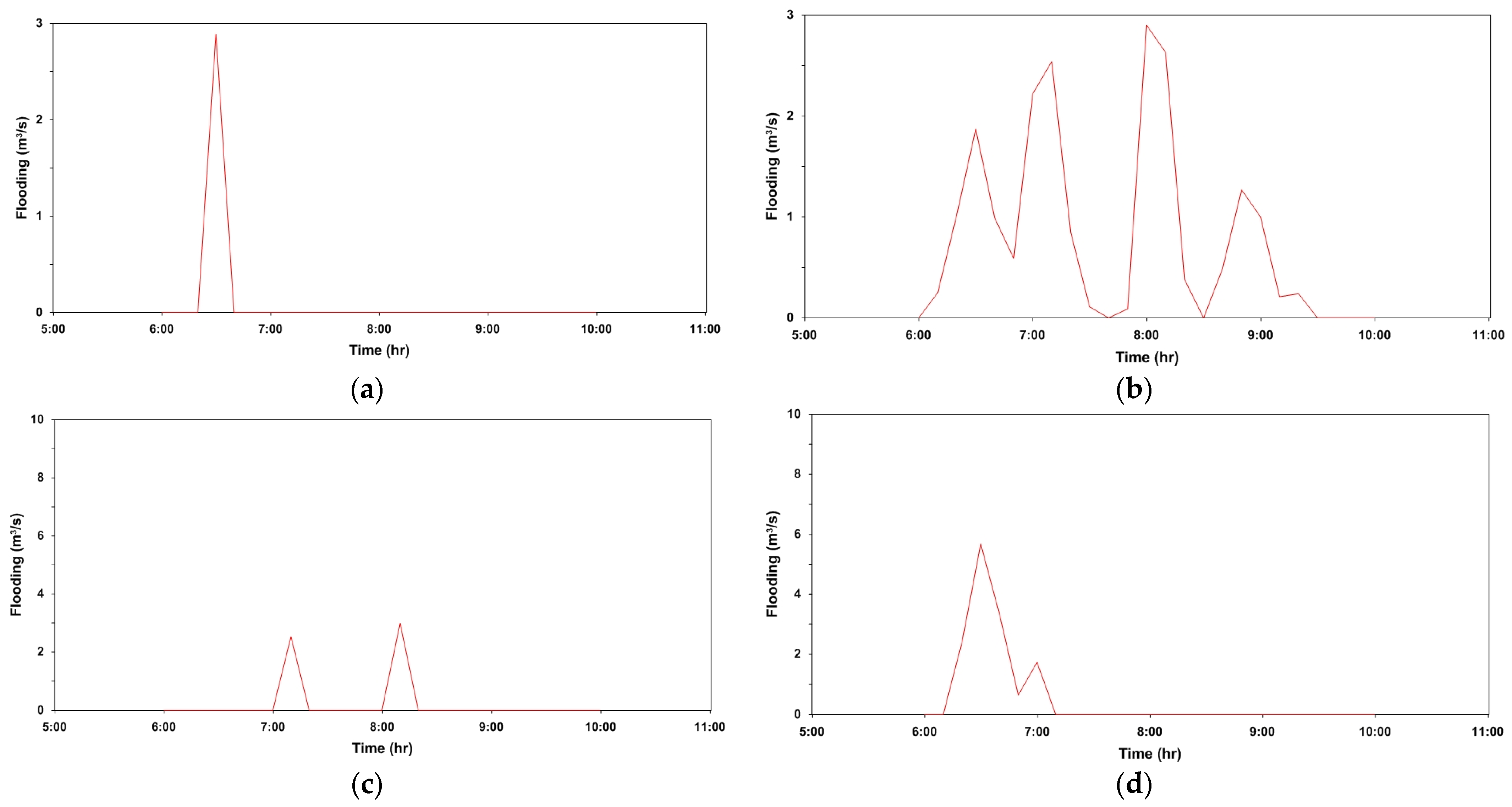
Figure 5. These results show that the automatic calibration method enables more accurate urban runoff analysis, and when automatic calibration is performed for parameters with a high sensitivity in the study catchment, the calculation time and accuracy increase, enhancing the efficiency. As a result of the urban runoff and 1D rainwater conduit analysis, overflow occurred for each scenario, as shown in
Table 6.
Figure 6 and
Figure 7 show the point at which overflow occurred in the results of the urban runoff analysis.
Figure 8,
Figure 9 and
Figure 10 present the amount of overflow that occurred from the overflow manholes of each scenario using a standard pipeline of 1200 mm or more for the rainfall event on 22 October 2013.
4.3. 2D Urban Flood Inundation Analysis
For the 2D inundation analysis, a DEM with a 2 m resolution was constructed, as shown in
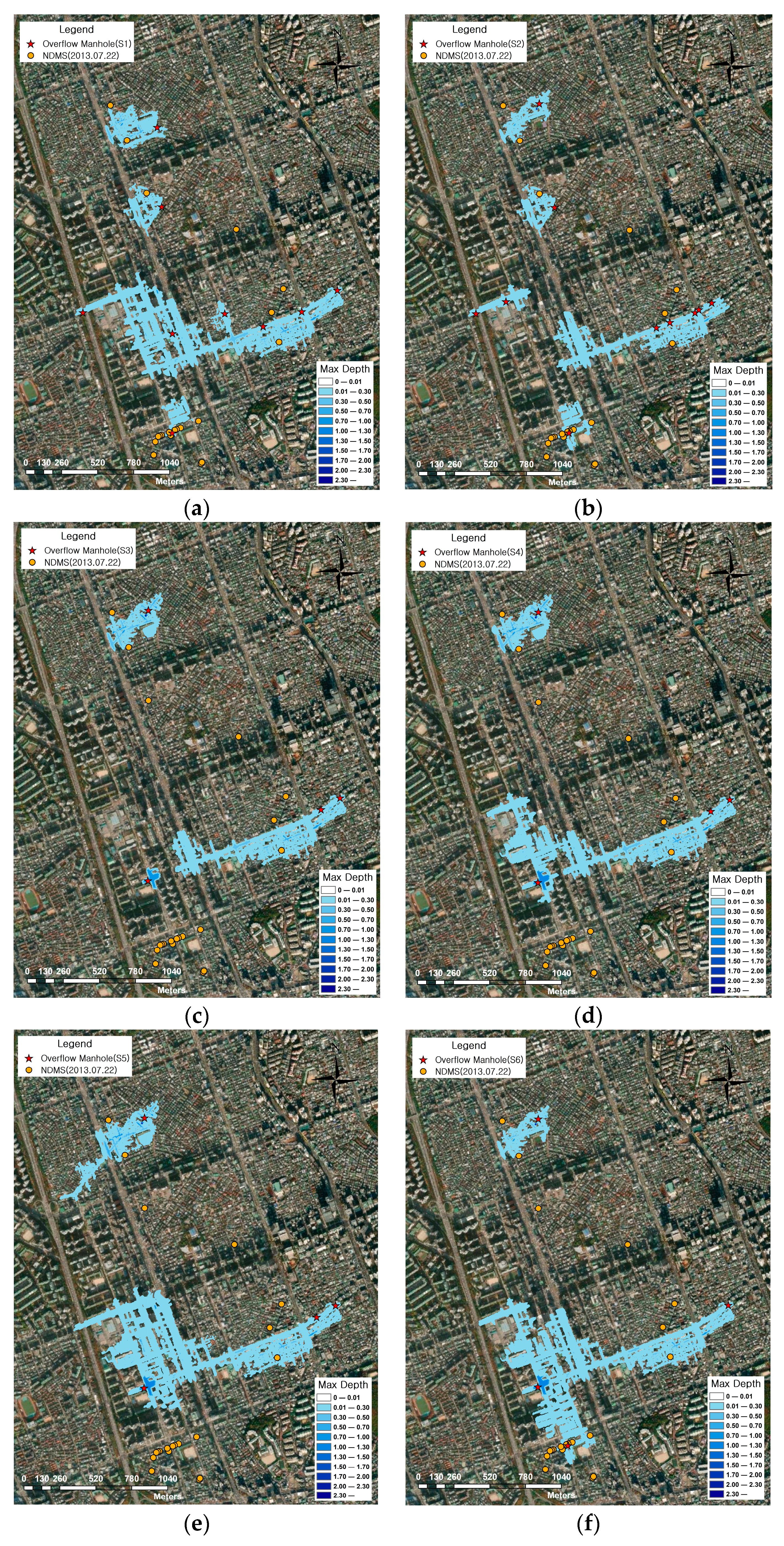
Figure 11, by reflecting buildings and roads in the LiDAR terrain data of Seoul. For the 22 July 2013 rainfall event, the simulated inundation for each scenario was compared with the NDMS (National Disaster Management System) reporting points and is shown in
Figure 12. The NDMS indicates the points at which residents reported flood damage.
Figure 13 shows the comparison of simulations and NDMS for the rainfall event on 21 September 2010. To verify the simulation results, the goodness of fit was calculated by comparing the NDMS and the predicted flood extent. The NDMS exists only as point data, so the fit was calculated according to the number of reporting points within the predicted flooding area.
As for the NDMS reporting points, there were a total of 20 points on 22 July 2013, and 117 points on 21 September 2010.
Table 7 shows the goodness of fit between the NDMS points and the predicted flood extent. The flood extent calculated using S6 included 13 NDMS points in the 2013 event and 82 points in the 2010 event. Among scenarios S4 to S6, in which automatic parameter calibration was performed, S6 accurately simulated the manhole overflow location, and thus the fit was the highest, as shown in
Table 7. In the nonverified scenarios, namely S1 to S3, overflows occurred at more points in S1, which was divided by the largest number of sub-catchments, than in the other scenarios (S2 and S3), and showed a higher goodness of fit.
5. Discussion
In this study, the parameters to be reflected in the automatic calibration were determined through sensitivity analysis. In addition, the accuracy of each scenario was compared and analyzed to improve the usability of the model in practical application; this was in order to solve the difficulty of increasing the time required to construct input data and the uncertainty as the number of sub-catchments increased.
(1) The sensitivity of the parameters in the study area was in the order of Manning’s roughness coefficient for conduits, the roughness coefficient of the impervious area, the width of the catchment, and the roughness coefficient of the pervious area. Therefore, it was found that the urban runoff analysis, considering the parameters with a high sensitivity in the watershed, had a higher accuracy and efficiency than the number of parameters.
(2) As a result of comparing the simulated scenarios without optimizing the parameters for the difference in the number of sub-catchments, the difference between the RMSE and RPE was found to be small. Therefore, considering the efficiency of topographic data construction and the calculation time, it was found that the S3 scenario reflecting a more than 1200 mm pipeline among S1, S2, and S3 was most suitable.
(3) When comparing scenarios using automatic calibration, the RMSE decreased by up to 2.37 cm (S3–S6) and RPE by 22.04% (S2–S4). For watersheds where parameter optimization is valid, it was found that the accuracy can be improved by reflecting only the main pipelines and manholes.
(4) As a result of considering the parameters in connection with the 2D inundation analysis, S6 was the most accurate, with 65.0% and 70.1%, and the fit of the scenario using a 1200 mm pipeline, not considering S6, was 20% and 43.6~66.7%, respectively; this was lower than S1 reflecting a 450 mm sewer pipe. Scenarios in which automatic calibration is performed, such as S6, may reflect the overflow point, but otherwise, a large error may occur. Therefore, scenarios into which a large number of sub-catchments are divided can result in overflows occurring at many points, resulting in reduced calculation errors; therefore, attention may be required when determining sub-catchment division and manhole reflection.
6. Conclusions
This study analyzed the sensitivity of key parameters in urban runoff and conduit modeling using PEST, and proposed a method with which to more effectively and accurately analyze urban runoff and flooding through the construction of runoff analysis scenarios. Since both accuracy and promptness are required for flood forecasting and warning, simulations were conducted using manhole water levels in the pipe network for actual rainfall events in five sub-catchments of the Banpo drainage area for a comprehensive comparative analysis of their efficiency. The main research findings are as follows.
(1) The sensitivity of major parameters was estimated by conducting urban runoff analysis linked to PEST. The study catchment was constructed using three topographical data cases, and four parameters were used for uncertainty and sensitivity analysis. The selection of parameters was determined according to the basin width, roughness coefficient of impervious and pervious areas, and Manning’s roughness coefficient for conduits, using previous research results.
(2) It was found that the urban runoff analysis that optimized the parameters with high sensitivity in the study area had high accuracy and efficiency.
(3) When comparing the accuracy according to the number of considered parameters, S5 and S6, which were automatically calibrated using three or four parameters, showed a lower RMSE and RPE as a whole. However, when the number of estimated parameters was greater than the number of observations, the accuracy of the optimization was lowered.
(4) In order to compare the accuracy of each scenario using the 2D flood inundation model, the localized rainfall that occurred in the study area in 2010 and 2013 was applied and compared with the NDMS data. S6 was the most accurate, with 70.1% and 65.0%, respectively. In the uncalibrated scenario, overflow did not occur in the manhole, but overflow occurred in S6, showing higher accuracy.
A sensitivity analysis for the main parameters of the study area and a scenario considering the results were created. The optimization of the parameters increased the accuracy of the runoff analysis and reduced the calculation time. In particular, S6 was more accurate than other scenarios in both 1D urban runoff analysis and 2D surface inundation analysis. Therefore, in the watershed in which automatic calibration is possible, it is expected that the division of the sub-catchment reflecting only the main sewer pipe after automatic calibration using high-sensitivity parameters can improve the accuracy and efficiency.
However, if parameter optimization is difficult due to a lack of observations, it is necessary determine whether the sub-catchment should be divided and the manhole should be reflected. In addition, this study had limited rainfall events that could be applied to the runoff and flood inundation analysis after the water level gauge was installed in the manhole. It is expected that more accurate flood prediction will be possible if a 1D–2D linkage analysis is performed considering various rainfall events in the future. In addition, if urban flood prediction is connected with machine learning, which is now widely used, it is expected that a more practical real-time urban flood forecasting and warning system will be established.
