Modeling Aquifer Responses from Flash Flood Events through Ephemeral Stream Beds: Case Studies from Saudi Arabia

Abstract

The determination of groundwater recharge (GWR) with an appropriate method is among the main subjects of groundwater resource management. This research is an event-scale quantitative assessment and a development of a water balance model of an aquifer response resulting from flash flooding and infiltration from the ephemeral streambed of some representative basins in Saudi Arabia. The methodology employed in the water balance analysis of this study starts with surface runoff rather than rainfall as in the literature, since the recharge process mainly occurs from runoff on the ground surface. A conceptual model of the local surface–subsurface interaction is developed to estimate the effective aquifer response (AR). The annual cumulative groundwater recharge (GWR) depths vary from 1.22 m to 6.97 m, with an average rise of 4.24 m at the studied wells; most of this happened following the May and April flash flood events. The results show also similar profile patterns and timings for most of the water level rises and falls. An average root mean square error (RMSE) of 0.46 m is obtained from the simulations and the coefficient of determination (R²) values range from 0.57 to 0.99. The results verified that the daily simulated groundwater elevations have shown very good agreement with the observed daily groundwater elevations over a time span of one year. In this work, the key issue to interpret the GWR depth from individual well samples is whether the model on the samples fits the measured groundwater level within the experimental runoff reaches (ERRs). The time steps (Δt) of the GWR simulation process are significantly affected by the high variability in the aquifer characteristics, as shown for the hydraulic conductivity values ranging from 5.3 m/day to 438 m/day within ERRs. This study highly recommends that groundwater recharge studies be site-specific. Otherwise, the extrapolation of the results even to adjacent basins is questionable.

1. Introduction

Since nature is complex, and each hydrological region is unique [1], precipitation that can recharge aquifers in arid regions would not be different from humid regions [2]. The streams in natural channels of arid and semi-arid regions are usually ephemeral, where flow occurs only following rainfall events. When a flood occurs, the volume of runoff and level of surface water will be reduced due to transmission loss (TL) along the streambed. Some part of this loss recharges the alluvial aquifer along the streambeds.

Streambeds are sediments covering alluvial aquifers. They are distinct geographic features comparable to soils and surficial geologic materials within watersheds with a relatively constant volume. For a given precipitation event, the topography within watersheds interacts with surficial geology to create both spatial and temporal seasonal patterns of stream exchanges with groundwater via streambeds [3].

In this regard, the determination of the amount of groundwater recharge (GWR) through these streams with appropriate methods is among the main subjects of groundwater resource management and sustainable development for any country [4,5,6]. However, as stated by many researchers [7,8,9,10,11], estimating the quantitative surface–subsurface water balance and exchange in arid and semi-arid regions is a challenging task. Among the main reasons, there is the high degree of rainfall characteristics’ variability, the inadequacy of continuously recorded data, the complexity of defining surface flow–recharge connections because of the potential nonlinearity, and the late response time of the groundwater table.

To estimate GWR, several complex models have been used for the estimation of GWR [12,13,14] as its direct measurement is nearly impossible and it is hindered by the significant uncertainty in different results [15,16]. Various methods require extensive fieldwork, while others involve the development of sophisticated models [17,18]. Hydrological budgets, water table fluctuations, numerical models, and tracer techniques are commonly used techniques [17]. Moreover, water-budget methods are applicable over any space and time scale [1,19,20].

Regarding the basins in the southwestern region of the Kingdom of Saudi Arabia (KSA), several investigations have been conducted to figure out channel losses and groundwater recharge from wadi beds (ephemeral channels). Among these studies [21,22,23,24], all have indicated that channel bed infiltration was very high and was influenced by the streambed characteristics, soil properties, and flood hydrographs. Since these parameters act interdependently, none of these studies arrived at simple models to estimate the magnitude of channel loss and the resulting GWR.

Some studies like [25,26,27,28] have addressed the subject of infiltration from wadi channels using analytical or numerical methods. So far, modeling the aquifer response because of recharge from flooding events and validating this model remain unsolved as far as our knowledge is concerned. Additionally, catchment-based studies can lead to erroneous estimates of GWR, since most of the land cover may not allow infiltration. Thus, to obtain reliable estimates, the where and when of the recharge should be identified. None of the above-mentioned articles include these issues.

The point-based vertical groundwater seepage rate approach was used by [29]; the study was conducted within a 2.5 km-long and 6.5 m-wide sandy streambed in North Carolina (USA). They estimated the Darcy velocity, v = KJ, where K (m/d) is the hydraulic conductivity and J is the hydraulic head gradient (dimensionless). Regarding this vertical infiltration model, [30] simply applied Darcy’s law and suggested a straightforward model for water moving through uniformly homogenous soil. This model performs best when the wetting front is somewhat sharp or distinct throughout the infiltration process. As opposed to fine-textured soils, coarse-textured soils are more likely to experience such a clear wetting front, and initially dry soil is more likely to do so than initially wet soil. Additionally, the model performs best when the wetted area’s soil texture is homogeneous and when air entrapment, surface crusting, and soil swelling have little to no impact on the infiltration process [31].

To identify useful parameters and to recognize the prominent event-scale vertical seepage mechanisms in the study area, a conceptual model of the local recharge processes is developed. Many studies like [1,32,33] strongly suggest the importance of developing a conceptual model of recharge processes as a first basic step in the beginning of any recharge estimation and evaluation study. It is also vital for selecting suitable GWR methods and obtaining meaningful estimates. Nevertheless, this process can be difficult and complicated by both natural and anthropogenic factors [1].

In this article, a simplified yet effective mathematical model is proposed and applied to estimate the aquifer response from flash flood events through ephemeral channels. A mass balance model is used to assess the aquifer recharge and groundwater level rise from flash flood events through the principal wadi bed of three representative basins (Habawanah, Yiba, and Tabalah) located in the southwest of the KSA. Along with modeling the aquifer response following flash flooding events, the developed model is validated using measured groundwater elevation data obtained from wells in the vicinity of the streambed. In the selected experimental runoff reaches, the direct relationship between the runoff rates with sub-surface recharge coming from TL as an aquifer response (rise in the water table) is estimated.

Accordingly, we have developed a detailed conceptual model that can figure out the spatial and temporal aquifer recharge processes and their mechanisms in the ephemeral streams during flash flood events. The model takes into consideration the storage in the unsaturated zone that is hydrologically the main factor controlling water movement from the land surface to the aquifer. This zone strongly affects the rate of aquifer recharge and is critical for the management of groundwater [30,34,35].

2. Materials and Methods

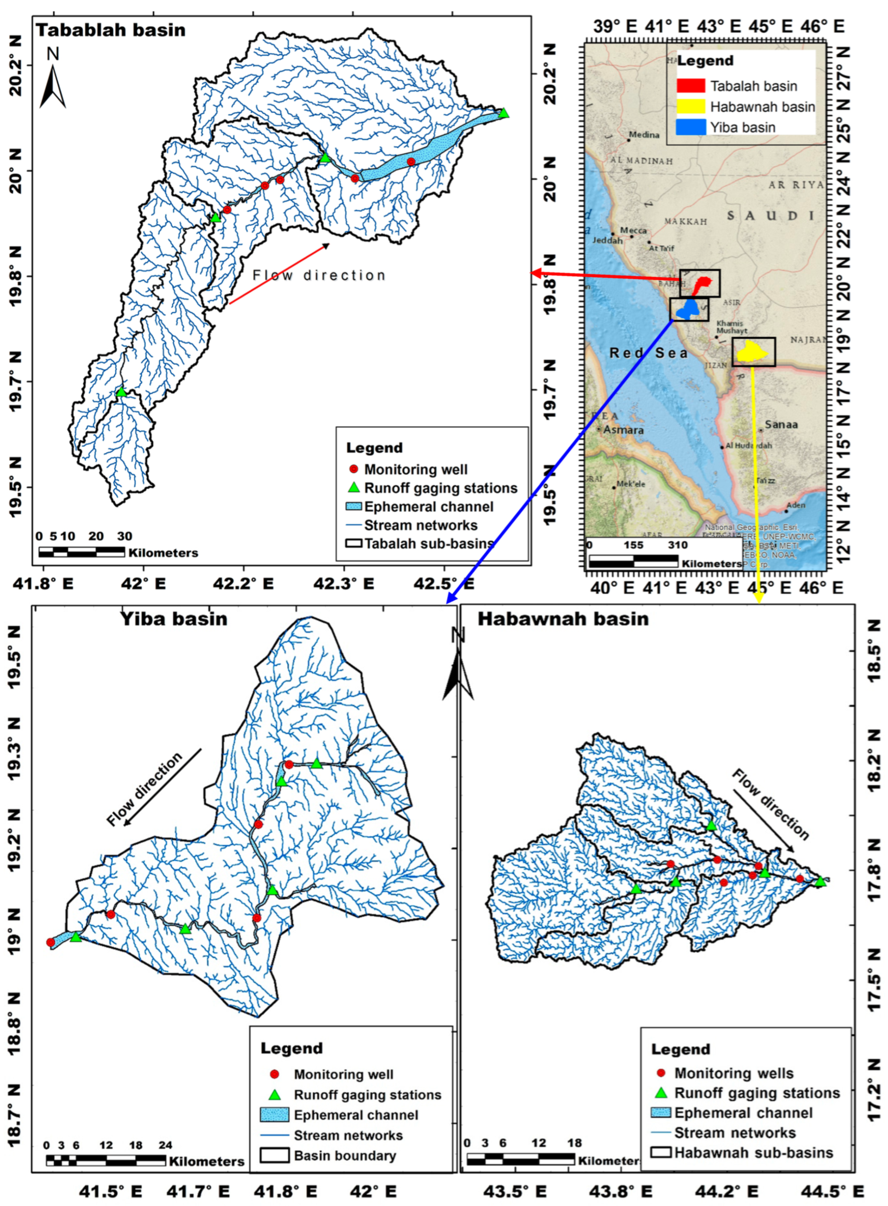
2.1. Description of the Study Area

This study was conducted via quantitative estimation and modeling of a principal wadi bed aquifer recharge and groundwater level rise from flash flood events using simple and operative methods in three representative basins (Habawanah, Yiba, and Tabalah) located in the southwest of the KSA (Figure 1).

Generally, this region is known for a high degree of rainfall variability in space and time. The wet season covers November to April, whereas the dry season covers June to September [36]. Due to the effect of climate change on seasonal rainfall, the rainfall slightly increased during 1979–1993 and significantly decreased during 1994–2009 [37].

Figure 2 shows sample plots modified from [38] for two rainfall stations (SA003 and SA004) in Figure 2a,b, that belong to the Ministry of Environment, Water and Agriculture (MEWA) and are located in the vicinity of the study basins. It summarizes the time series of the monthly rainfall depth over the period of 1967 to 2005. It shows the high degree of variability in the rainfall. The figure also shows the depth–duration–frequency (DDF) curves using data from MEWA in Yiba basin. These curves are presented in Figure 2c,d. It shows the DDF for return periods from 2 to 200 years which is estimated from the station data, and the dots are the actual rainfall depths of the events that already happened during the Dams and Moore project in the period of 1984–1987. The curves show that the majority of the rainfall events are below the 2-year return period; however, there are some extreme events that are over the 200 years return period, confirming the high degree of variability in temporal rainfall in the region.

MEWA has already recognized the three basins (Figure 1) as being among the country’s principal representative basins. A mountain range that runs parallel to the Red Sea coast in the southwest of the Kingdom defines the basins, whereby some of which drain inland and others drain toward the sea [4]. This aquifer response modeling has focused on the main streams of the three basins (

Table 1. The main features of the three representative basins.

Basin	Basin Area (km2)	Range of Altitude Elevation above Mean Average Sea Level (m.a.s.l)
Habawnah	4930	1155 to 2738
Yiba *	2830	68 to 2701
Tabalah	1270	1200 to 2440

Note: * flows to the Red Sea.

). The important hydrogeological basin characteristics of each of them are discussed as follows.

The basins are located in the Arabian Shield and underlain principally by Precambrian crystalline rocks. The only known significant aquifer systems in the basins are contained within the valley infill alluvium; specifically, in the Principal Wadi Alluvium (PWA) [22,23]. The stream networks collect the majority of surface flow to the lower PWA that is contained within the drainage line of their large tributaries (Figure 2).

Indeed, the upper halves of the basins are characterized by the occurrence of a series of alluvium-infilled sub-basins. However, each of them contains a discrete groundwater system, so the hydraulic continuity between and among sub-basins is varying in magnitude, as the connecting channels are usually narrow in the upstream of the basins, and the alluvium is thin. Therefore, this study has focused on the lower reaches in the basins, where runoff gaging stations are available, such as N-406 and N-407 for Habawnah (Figure 3a).

2.2. Groundwater System of the Study Area

Previous groundwater studies, like [21,22,23,25,26,28,38], in the region have identified that the aquifer is generally composed of wadi infill, wadi alluvium, and coastal plain sediments containing the only significant groundwater systems. According to the Dams and Moor report, project investigation drilling, previous studies, and data from the wells inventory, all showed that groundwater could also be obtained or lost, often readily, from fractured bedrock beneath the alluvium.

Hence, the only known major source of recharge to the water table aquifers in the alluvium is from surface flows in the channels; this surface–subsurface interaction modeling work was focused on the hydrogeological assessment of the water system associated with the major alluvial-infilled channels. Drilling logs have indicated that the upper regions of all the wells consist of sand, gravel, or silt mixture, which are all high hydraulic conductivity profiles. The upper halves of the basins are characterized by the occurrence of a series of alluvium-infilled sub-basins. Nevertheless, the hydraulic continuity between and among sub-basins is limited as the connecting channels are usually narrow, and the alluvium in them is thin.

2.3. Data Collection

Hydrological data (rainfall, inflow, and outflow data), geological data (well locations, aquifer type, lithology, pump test data, monitored groundwater levels and well depth), and soil physical parameters (hydraulic conductivity, porosity, moisture content, etc.) were collected from [22], an exclusive water status project carried out at selected basins in Saudi Arabia between 1984 and 1988. The main data of this study have focused on the selected experimental runoff reaches (ERRs) as shown by Figure 4c as a sample.

As illustrated by the above figure, the runoff event happened on 16 April 1986 that leads to rise up the groundwater level (Figure 4d). The inflow volume of 2.37 Mm³ (Figure 4b) reduction, i.e., the TL to volume of 1.83 Mm³ at the outflow (Figure 5a) clearly showed this effect. In this article, we have attempted to model this surface–subsurface interaction.

For all experimental reaches in the three representative wadis with upstream and downstream gages were inspected to obtain a sample of runoff events from which TL could be determined reliably. Assumptions including, only events with inflow and outflow hydrographs; runoff and rainfall data indicated no tributary inflows to the reach, inflow hydrograph was greater than the outflow hydrograph; saturated groundwater level indicated sufficient storage capacity to allow free infiltration of runoff waters into the wadi beds; were used in selection of sample of runoff events for analysis.

This study has focused primarily on four experimental reaches found between gaging stations; N-406 to N-407 (Figure 4a), SA-423 to SA-424 and SA-422 to SA-401 (Figure 5b) and B-412 to B-405 to model the temporal fluctuation of groundwater table under PAW bed. Accordingly, the following runoff hydrographs were selected to model the aquifer response at the ERRs in the three basins (

Table 2. Selected runoff events for aquifer response analysis in the three basins.

Year	Basin	ERRs	No of Selected Runoff Events
1984	Yiba	(SA-423) to (SA-424)	10
1985	Yiba	(SA-423) to (SA-424)	5
1985	Yiba	(SA-422) to (SA-401)	9
1985	Habawnah	(N-406) to (N-407)	2
1985	Tabalah	(B-412) to (B-405)	6
1986	Tabalah	(B-412) to (B-405)	2

).

Thirty-four flood events (sixty-eight inflow and outflow of the reaches) (Table 2) were selected to determine an estimate of GWR rate and the resulting water level rise within the selected ERR. The events in Tabalah (B-412) to (B-405) were analyzed in three different monitoring wells (3-B-96, 3-B-97 and 3-B-98). The following Figure 5a,b show sample runoff hydrographs.

Continuously monitored groundwater level data at the monitoring wells as shown in Figure 6 are collected from [22]. They were used to validate the results with the actual water level profile. The following two figures (Figure 6a–c) show sample groundwater elevation profiles from each of the three basins.

Monitoring wells H-15-P (Habawnah basin); 6-T-103 and 6-T-106 (Yiba basin); and 3-B-96, 3-B-97, and 3-B-98 (Tabalah basin) were selected to run simulations and validate results of the temporal groundwater level fluctuation as a response to flood events within the experimental runoff reach (ERR). The peak discharges (Q) shown in the figures represent the inflow hydrographs at the channel reach.

The transfer of water from the ephemeral channel bed to the subsurface is mainly governed by the type of the channel bed materials, the soil moisture conditions at the start of a runoff event, the hydraulic conductivity (k), the depth of the groundwater table, and the depth and ponding time of water inundated on the ground surface.

Table 3. Selected hydraulic properties from field pumping tests.

Year	Basin	Well	Depth to Water before the Flood (m)	Bedrock Depth (m)	Hydraulic Conductivity (m/d)
1984	Yiba	6-T-103	6.54	14.0	624
1985	Yiba	6-T-106	7.23	9.75	5.0
1985	Yiba	6-T-106	7.46	9.75	5.0
1985	Habawnah	H-15-P	18.27	33.0	5.3
1985	Tabalah	3-B-96	4.35	35.0	17.0
1986	Tabalah	3-B-96	7.53	35.0	17.0
1985	Tabalah	3-B-97	4.35	14.4	438.0
1985	Tabalah	3-B-98	6.71	21.0	58.0

shows some characteristics of the soil profile at the streambed.

At the basin scale, the saturated hydraulic conductivity (k) is generally high with a range of k = 5.3 m/d–1806 m/d (not included in this study) in Habawnah, k = 5 m/d–624 m/d in Yiba, and k = 17 m/d–438 m/d in Tabalah. This difference clearly indicates the heterogeneity of the system. Table 2 shows the variability in the hydraulic conductivity measured from pumping tests within the basins.

The above paragraph discussed how the characteristics of the ephemeral channels in the three basins guarantee that a substantial amount of water could infiltrate into the unsaturated zone and then raise up the groundwater table based on large infiltration capacity.

2.4. Modeling Aquifer Response from Flash Flood Events through ERRs

To estimate the transmission losses occurring in the selected experimental runoff reaches (ERRs), inputs such as the runoff hydrograph data between two runoff stations, the location of the well between the two stations, the measured groundwater level data, the channel bed physical characteristics, and the aquifer physical parameters were required. The developed mathematical model used the input data to estimate channel bed losses from the given runoff and to estimate the water level rise in the unconfined aquifer beneath the ground surface Model details are given in the following sections.

2.4.1. Conceptual Model of GWR from Flood Events

This model (Figure 7) is intended to describe the basic recharge parameters, aquifer characteristics, boundary conditions, and variations in inputs and/or outputs of the system.

This conceptual model has enabled us to proceed to a mathematical model. Since most ephemeral streams have wide beds, the infiltration occurs typically vertically. Thus, the one-dimensional flow assumption is reasonable in the area [25].

The groundwater in fractured bedrock underlying alluvium was considered as belonging to the same aquifer system, as it is recharged from the overlaying alluvium material and acts as an extension of that material. This study was restricted to these aquifer systems under alluvial drainage up to the impervious bedrock.

As shown in Figure 8, the event-scale runoff–recharge modeling parameters were identified from the conceptual model of the local recharge processes that led us to obtain meaningful groundwater elevation rise $(\Delta h)$ estimates.

2.4.2. Event-Scale Runoff–Recharge Modeling in ERRs

The common water-budget methods over any space and time scale that are available in the literature [1,18,19] are commonly expressed as follows:

P = ET + ΔS + R_f + D

(1)

where P is precipitation; ET is evapotranspiration, which includes evaporation and plant transpiration; ΔS is the change in water storage in a column; R_f is the direct surface runoff (precipitation that does not infiltrate); and D is the drainage out of the bottom of a column. All components are given as rates per unit surface.

To develop a mathematical model between groundwater level rise due to runoff events, the measured yearly groundwater level response hydrographs reported by [23] were used as a base for such a modeling exercise.

In this article, we propose the following mass balance model (Equation (2)). The developed model links the surface water (flood hydrographs, evapotranspiration) with subsurface water (infiltration, unsaturated zone storage, groundwater flow, groundwater loss, and pumping) to estimate the aquifer response in the ERR. The model does not take rainfall via the traditional approach as mentioned in Equation (1); it starts from runoff events. The mass balance can be written as follows:

$$\left(I+G_I\right)-{(O+G}_O)-ET-Abs-GL=\frac{d{S}_G}{dt}+\frac{d{S}_u}{dt}$$

(2)

where I is the surface water inflow discharge (L³/T); G_I is the subsurface inflow discharge (L³/T); G_O is the subsurface outflow rate (L³/T); ET is evapotranspiration expressed as volume per time over the reach area (L³/T); Abs is the water abstraction discharge from wells (L³/T); GL is the groundwater loss rate (L³/T); $\frac{d{S}_G}{dt}$ is the rate of change in groundwater storage volume (L³/T); $\frac{d{S}_u}{dt}$ is the rate of change of the unsaturated zone water storage volume (L³/T); and t is time; O is the surface water outflow discharge (L³/T).

The infiltration (i) resulting from the surface water can be estimated as:

$$i=I-O$$

(3)

Thus, Equation (2) can be re-written as:

$$i+{{(G}_I-G}_O)-ET-Abs-GL=\frac{d{S}_G}{dt}+\frac{d{S}_u}{dt}$$

(4)

We assume $S_u=\alpha \ast S_G$ and $\alpha$ ≤ 1, where α is the unsaturated zone storage coefficient.

Then:

$$i+{{(G}_I-G}_O)-ET-Abs-GL=(1+\alpha )\frac{d{S}_G}{dt}$$

(5)

In a finite difference form,

$$\Delta S_G=\left[\frac{i+{{(G}_I-G}_O)-ET-Abs-GL}{(1+\alpha )}\right]\Delta t$$

(6)

since

$$\Delta S_G=\Delta h\ast L\ast {B\ast S}_y$$

(7)

where $\Delta h$ is the groundwater level rise; L is the length of experimental runoff reach; B is the width of experimental runoff reach; and Sy is the specific yield of the aquifer.

The head gain $(\Delta h)$ raises the WTE level. Therefore, the event-scale total groundwater recharge depth can be formulated using the final water balance formula in the aquifer system as follows:

$$\Delta h=\left[\frac{i+{{(G}_I-G}_O)-ET-Abs-GL}{(1+\alpha )L\ast {B\ast S}_y}\right]\Delta t$$

(8)

The final groundwater table following the runoff events $\left(WTE\left(t+\Delta t\right)\right)$ can be formulated as:

$$WTE\left(t+\Delta t\right)=WTE\left(t\right)+\Delta h\left(t\right)$$

(9)

In this paper, the above model is successfully applied at six wells located in different ERRs of the three basins. The groundwater level at any time (t) is WTE (t) and the groundwater level at the next time is WTE (t + ∆t). This value was obtained through considering the major possible losses such as evapotranspiration (ET), groundwater flow loss (GL), the unsaturated zone storage coefficient (α), and abstraction losses from pumping (Abs).

2.4.3. Time Step ($\Delta t$) of the GWR Simulation Process

In this modeling task, determining the time that water takes to infiltrate and reach the groundwater table is critically important. The famous Darcy law was applied, considering the sharp front moving vertically down through the aquifer system as applied by [36]. As the runoff starts at the channel surface, the wetting front is supposed to move like a piston displacement through a vertical soil profile.

The model, in this study, assumed some conditions, such as a homogeneous soil column, uniform antecedent water content, constant pressure head at the wetting front, constant groundwater reservoir level, and constant hydraulic conductivity in the wetting region (Figure 9).

In the vertical soil profile (Figure 9), the rate of the downward flow was formulated with ponding depth (H₁₎ and Darcy’s flux equation as:

$$q=k\frac{{Z+H}_1}{Z}=k\left(\frac{H_1}{Z}+1\right)$$

(10)

where q is the Darcy flux or Darcy velocity (m/s) and k: is the hydraulic conductivity (m/s).

Since H₁ is small compared to Z, it can be ignored. The vertical flux is equal to the hydraulic conductivity and the equation with the head gradient becomes:

$$q=k$$

(11)

This $q$ is called the Darcy velocity (specific discharge), which is calculated from the discharge rate per unit cross sectional area of the vertical pores medium. The seepage velocity is calculated as:

$$V_S=\frac{k}{n}$$

(12)

where n is the effective porosity of the medium.

From this velocity, the time step $(\Delta t)$ of the infiltrating water to reach the groundwater table is determined as follows:

$$\Delta t=\frac{V_S}{Z}$$

(13)

This time step has been used as a base to interpolate the measured daily groundwater level data over sub-daily time steps ($\Delta t)$ to link between the time scale of surface water runoff and the time scale of groundwater infiltration.

For parameter estimation, we have applied the Microsoft Excel 2010 Solver, which has grown to be the most extensively used and distributed general-purpose optimization modeling solution since its release in February 1991 [39,40]. In the target cell of a worksheet, the objective function is formulated as the root mean square error (RMSE) between the observed and modelled WTE for the whole year. The Excel solver acts on a set of cells to estimate the major losses (ET, GL, α, and Abs). The solver modifies the values in the user-identified adjustable cells to minimize the RMSE.

The Aquifer Recharge Model (ARM) accounts for four main losses to estimate the net water table elevations as presented by (Equation (8)), i.e., evapotranspiration from the whole system, water abstraction from wells, groundwater losses, and storage in the unsaturated zone. The events in Tabalah (B-412) to (B-405) were analyzed in three monitoring wells (3-B-96, 3-B-97, and 3-B-98). That means the six events for the year 1985 and the two events for the year 1986 were analyzed at different three wells within that ERR. The transmission loss (TL) was estimated from the volume of the inflow hydrograph (V_ups) and the volume of the outflow hydrograph (V_dws).

As presented in

Table 4. Aquifer response model analysis result through the ERR of the three basins.

Event Starting Date	Basin	ERR	Qp (m3/s)		Vups (103m3)	Vdws (103m3)	TL (103m3)	Annual Aquifer Reponse Elements
			Ups	Dws				ET (m/d)	α	Abs (m/d)	GL (m/d)	GWR (m)
07/04/86	Habawnah	N-406/N-407 (Well # H-15P) L = 19.6 km	32.82	22.85	944.94	414.83	530.11	0.74	0.15	0.68	0.07	1.22
16/04/86			149.57	118.33	2373.85	1830.98	542.87
12/05/84	Yiba	SA-423/S-424 (Well # 6T-106) L = 33.4	205.49	67.07	1413.00	724.24	688.76	2.37	0.15	0.22	0.05	3.75
13/05/84			88.73	23.82	1270.92	500.68	770.24
16/05/84			100.00	22.94	1117.62	375.76	741.86
21/05/84			177.62	127.65	1179.19	1160.37	18.82
19/08/84			133.29	13.35	1120.47	237.17	883.30
29/08/84			38.28	15.24	331.69	241.18	90.51
10/09/84			175.79	40.57	1084.11	406.60	677.51
19/09/84			135.14	30.68	1393.10	598.94	794.16
20/09/84			182.30	66.29	1491.30	850.58	640.72
17/11/84			78.83	7.74	617.93	259.37	358.56
01/05/85	Yiba	SA-422/S-401 (Well # 6T-103) L = 10.8 km	111.70	57.35	376.37	329.08	47.29	1.10	0.15	0.02	0.00	6.97
05/05/85			19.17	8.60	112.51	98.62	13.89
12/07/85			26.67	17.35	137.37	135.00	2.37
15/08/85			157.60	66.87	728.09	441.58	286.51
16/08/85			117.00	59.00	562.03	344.85	217.18
25/01/85	Tabalah	B-412/B-405 (well # 3-B-96) L = 22.8 km	45.60	14.47	484.73	203.45	281.28	1.27	0.15	1.27	0.90	4.24
05/04/85			18.45	2.75	416.73	29.47	387.26
10/04/85			80.67	18.76	707.29	443.81	263.48
11/04/85			223.35	36.38	2207.53	2130.21	77.32
23/04/85			3.03	0.00	149.76	0	149.76
01/05/85			5.72	0.00	238.95	0	238.95
25/01/85	Tabalah	B-412/B-405 (well # 3-B-97) L = 22.8 km	45.60	14.47	484.73	203.45	281.28	2.04	0.15	1.67	1.31	4.27
05/04/85			18.45	2.75	416.73	29.47	387.26
10/04/85			80.67	18.76	707.29	443.81	263.48
11/04/85			223.35	36.38	2207.53	2130.21	77.32
23/04/85			3.03	0.00	149.76	0	149.76
01/05/85			5.72	0.00	238.95	0	238.95
25/01/85	Tabalah	B-412/B-405 (well # 3-B-98) L = 22.8 km	45.60	14.47	484.73	203.45	281.28	1.57	0.15	1.42	1.06	4.27
05/04/85			18.45	2.75	416.73	29.47	387.26
10/04/85			80.67	18.76	707.29	443.81	263.48
11/04/85			223.35	36.38	2207.53	2130.21	77.32
23/04/85			3.03	0.00	149.76	0	149.76
01/05/85			5.72	0.00	238.95	0	238.95
04/04/86	Tabalah	B-412/B-405 (Well # 3-B-96)	9.38	0.00	151.31	0	151.31	1.10	0.14	0.02	0.00	2.80
07/04/86			54.80	19.41	864.14	236.05	628.09

, the TL is determined from the difference of the volumes (V_ups and V_dws) at the two ends of the reach. The annual aquifer response elements (ET, GL, α, Abs, and GWR) are used to solve Equation (8). Actually, GWR represents the head gain $(\Delta h)$.

3. Results

Table 4 summarizes the results of the ARM through ephemeral channels of the three basins.

The GWR, represented as groundwater level rise, was 1.22 m, 3.75 m, 6.97 m, 4.24 m, 4.27 m, 4.27 m, and 2.80 m in the studied wells. It means that the annual aquifer recharge came from the runoff events within the selected ERR. The value of α (the unsaturated zone storage coefficient) indicates nearly 15% of the infiltrating water was stored in the vadose zone.

The following water level profiles were generated from the model (Figure 10). The figure shows samples of the daily time series of the water table response at some wells to flood events over a time span of one year. The temporal water head gained from the infiltration following runoff events was obtained through the cumulative addition of the water level rise $(\Delta h)$ to the reference elevation of each monitoring well. This gives the annual gross water table elevations, WTE (t), at each site. The figure shows the components of the groundwater elevations and losses. Each profile in the figure shows a component in the losses, e.g., the blue line shows the water table elevation without losses (gross WTE), the black profile shows the measured WTE, the dotted green shows the WTE profile with ET losses, the purple shows the WTE profile with ET and Abs losses, and the red shows the net WTE profile. These were determined accounting for the abovementioned losses separately and as a whole to show the final annual water table elevations shown in Figure 10.

In Figure 10, WTE (t) gross is the gross water table elevation before the subtraction of the losses; WTE (t) measured is the daily observed water table elevation; WTE (t) − ET is the water table elevation after the subtraction of the evapotranspiration loss; WTE (t) − ET − Abs is the water table elevation after the subtraction of the evapotranspiration and abstraction losses; WTE (t) net is the net water table elevation after the subtraction of all considered losses. The data profile is the continuously recorded daily groundwater elevations through 1984 to 1986 from ground reference elevations used to validate the model.

The measure of the model accuracy is made through calculating the difference between the components of the water table elevations (WTEm) estimated by the model and the observed water table elevation (WTEo). The root mean square error (RMSE) test is estimated as follows:

$$\mathrm{R}\mathrm{M}\mathrm{S}\mathrm{E}=\sqrt{\frac{1}{\mathrm{n}}\sum _{\mathrm{i}=1}^{\mathrm{n}}\left[{\left(WTEm\right)}_i-{\left(WTEo\right)}_i\right]}$$

(14)

The results of RMSE for all loss components and the wells considered in the region are presented in Figure 11. It shows the discrepancy is minimal between the water table elevations estimated by the model and the observed water table elevation. The average RMSE value is 0.46 m for the events considered in the study.

The RMSE is calculated for all components of water table elevation at daily scales., i.e., WTE (t) gross is the gross water table elevation before the subtraction of the losses, WTE (t) measured is the daily observed water table elevation, WTE (t) − ET is the water table elevation after the subtraction of the evapotranspiration loss, WTE (t) − ET − Abs is the water table elevation after the subtraction of the evapotranspiration and abstraction losses, and WTE (t) net is the net water table elevation after the subtraction of all considered losses.

Figure 12 shows a comparison between the observed WTE and modeled WTE. In the figure, the observed water table elevation is plotted against the modelled water table elevation for a period of one year based on a daily time step. Some of the wells show high agreement between the observation and the model (wells H15P, 3-B-96, and 6-T-106); however, there are some wells that do not show relatively good results (e.g., wells 6-T-103, 3-B-96, and 3-B-98).

The statistical test results presented in Figure 11 and Figure 12 reveal that the proposed ARM fits relatively well with the observed groundwater elevation at the study sites. The R² values range from 0.57 to 0.99, which proves the soundness of the model.

4. Discussion

Table 4 shows that the GWR depth estimated from the annual water balance elements showed that the largest portion of the surface runoff has gone to join the groundwater table under the PAW. The GWR raises the water table by with a minimum of 1.2 m to a maximum of 6.97 m for the studied events. This means that the annual cumulative water depth of aquifer recharge came from the whole runoff events, within the selected ERR. In all cases, the α (the unsaturated zone storage coefficient) value indicates nearly 15 percent of the infiltrating water was stored in the vadose zone.

The results of Figure 10 show that the groundwater levels rise up for all cases following each runoff event. This reveals that there is a direct and immediate connection between surface- and groundwater in PAW. The cumulative annual groundwater elevation rose about 1.22 m from two events in Tabalah, of which the event peak flows were 149.57 m³/s and 32.8, respectively (Figure 10a); there was a rise of 3.75 m from ten runoff events in Yiba basin (Figure 10b), and so on. The results showed the effect of the number of events on the GWR. However, the largest GWR depth of 6.97 m is found in the reach between station SA-422 inflow and station SA-405 outflow (Yiba basin) due to the fact that they have the largest reach area.

The result of the analysis has revealed successful results for the selected flood events. The modeled groundwater elevations have shown a relatively very good agreement with the measured temporal groundwater elevations. They have followed similar patterns and timings for most of the rises and falls. It is also clear from the results that the aquifer level rises following each event and the magnitude of the water level rise is directly proportional to the magnitude of the peak discharge. The majority of the significant runoff events that result in aquifer recharge have happened in the months of May and April.

The larger the number of runoff events and the longer the length of the streambed wadi channel, the higher the transmission losses and therefore the increase in the water table level. The highest loss component is due to evapotranspiration, which is expected due to the aridity of the region.

The groundwater level has direct responses following the runoff events through the ephemeral channels of the three representative basins (Habawanah, Yiba, and Tabalah) in the southwest of the KSA. This proves that transmission losses from surface runoff are the main and even the only source of groundwater recharge in the downstream area of the basins.

The magnitude of the TL analyzed in this study has been highly affected by the flow volume, the duration of the runoff, and the area of inundation (the entire water level that develops as a result of floods is on ordinarily dry ground) in the ERRs. As shown by the results in Table 4, the larger the number of runoff events and the longer the ERRs, the higher the TL and other losses. Following each runoff event, the magnitude of the water level rise is proportional to the volume of the inflow hydrograph.

Temporally, infiltration into the principal wadi alluvium has occurred only during the period of flood events available in the channel. The majority of significant runoff events which result in aquifer recharge have happened in the months of May and April. Thus, the abstraction and well development works should keep this under consideration to achieve better management of the aquifer.

During the flood period, there will be a large area of inundation and, consequently, an opportunity for infiltration. The observed runoff events are mostly unsteady flow, rapid rise, and fall of water levels during each runoff event. Therefore, the depth and the area of inundation change rapidly in a short time span.

The method of estimating the time step proved that the wetting front reaches rapidly to the groundwater table. Thus, the one-dimensional (vertical) movement of the sharp front assumption is acceptable. However, after the wetting front reaches the water table, this assumption could not work. Therefore, it needs another time step analysis in the saturated groundwater zone below the water table, which is beyond this study.

Spatially, the only known significant aquifer system in the study basins were contained within the valley infill alluvium; specifically, in the lower stream PWA, as shown by Figure 3a–c. Therefore, the commonly used catchment-based aquifer recharge methods may lead to erroneous estimates and unacceptable generalization.

The local hydraulic conductivity and the position of the initial groundwater table are the key parameters to estimate the time step $(\Delta t)$ of the GWR process; this time step is used to trace the wetting front until it reaches the groundwater table. The water table at or near to the surface has inhibited TL, for deep water table infiltration occurred, and the loss rate was noted to decrease.

High variability in aquifer characteristics and hydraulic properties like the hydraulic conductivity (from 5.3 m/d to 1806 m/d), even within a basin (Table 2), was identified. Thus, it was recognized that the role of groundwater in the overall water balance of a given region would be dependent on the particular site-specific hydrology of the area, which can vary from basin to basin. Therefore, the extrapolation of groundwater data even to adjacent basins could be difficult. Such extrapolation is yet an essential part of groundwater management.

For similar conditions, like in the Tabalah basin, the groundwater table rise showed almost the same depth (4.27 m) for the two wells (3-B-97 and 3-B-98) that are in the same ERR. This clearly indicated the high accuracy of the model.

The R² values ranging from 0.57 to 0.99 proved to some degree the soundness of the model.

5. Summary and Conclusions

The methodology employed in the water balance analysis of this study starts with surface runoff rather than rainfall as in the literature, since the recharge process mainly occurs from runoff on the ground surface.

The developed conceptual model links the surface runoff with the aquifer recharge model (ARM). Practitioners can use this conceptual model to develop management and protection strategies and to make predictions of the water level rise due to runoff passing between hydrological stations

In the ARM, the movement of the wetting front in the unsaturated zone is determined based on the Green and Ampt model.

The annual cumulative GWR depths in the current study ranged between 1.22 m to 6.97 m for the experimental wells used, most of which happened following flash flood events in May and April. The model results show similar patterns and timings for the water level rises and falls, RMSE, and R² values verified from site to site. The daily simulated groundwater elevations have shown relatively very good agreements with the observed daily groundwater elevations for most of the wells.

The time steps (∆t) of the GWR simulation process are significantly affected by the high variability in aquifer characteristics, as shown for hydraulic conductivity values ranging from 5.3 m/d to 438 m/d within a reach. This is due to the high spatial variability of the hydraulic conductivity observed in the literature, e.g., the field experiments and numerical simulations performed by [41] in the lower Heihe River in northwestern China, which is characterized by a hyper-arid environment with extremely hot summers and severely cold winters.

Due the high variability in hydraulic conductivity among the sites, this study highly recommends that groundwater recharge studies must be site-specific. The extrapolation of the results to adjacent basins is questionable.

The α value = 15% indicates the fraction of the infiltrating water stored in the vadose zone of the vertical column in the studied wells. This means that 85% of the runoff water is recharged and joins the aquifer system to raise the water table. In a similar event-scale approach, [38] reports 77% of total spatial average precipitation is transferred to infiltration at a catchment scale based on a water balance model in the area using Soil Conservation Service (the SCS method).

Since the downstream Principal Wadi Alluvium (PWA) contains a significant aquifer system in the study basins, the abstraction wells should be built in the downstream of the PWA. This model can be used for other areas with appropriate parameter adjustments. The model could be improved and incorporated into two-dimensional and three-dimensional groundwater flow models to study aquifer management. Besides, this work is a contribution to establish stream bed hydrology in future predictions of stream exchanges with ground water; as highly recommended by [42].

The findings of this study can aid the local water resource management authorities in allocating the spatial and temporal distribution of ground water availability resulting from flash floods.