Abstract
The use of either analytical or numerical models of groundwater inflow into a tunnel, ignoring the excavation process, will result in inaccurate prediction. More researchers have begun to study prediction methods with temporal and spatial variables, in accompaniment with the tunnel excavation progress. The hydrogeological parameters significantly affect tunnel inflow prediction; thus, it is always worthy to carry out an inversion analysis when the inflow rate observation is available for the excavated part of a tunnel. Based on a transient analytical model and the Trust Region Reflection (TRR) algorithm, this paper proposes a Dynamic Parameter Calibration (DPC) method to sequentially optimize parameters for a tunnel that is divided into several sectors. The results of two case studies indicate that the fitting effects by DPC are significantly improved compared with the empirical trial-and-error method, indicating good optimizations. The proposed scheme can conduct calibration simultaneously for multiple tunnel sectors and also several optimizations for the same sector. The parameter optimization results reflect the lithologic heterogeneity of different strata. Parameter sensitivity analysis proves that the hydraulic conductivity K has a greater influence on water inflow calculation than the specific storage coefficient S.
1. Introduction
The study of tunnel water inflow has always been a hot and difficult point of concern. In the process of tunnel construction, accurate prediction of water inflow can effectively reduce the risk of water inrush disaster and ensure the safety of tunnel construction and excavation progress. Scholars have systematically summarized the calculation methods of water inflow and introduced in detail the theoretical principles, assumptions, advantages and disadvantages, and applicable conditions of the existing calculation methods of tunnel water inflow [,]. When using analytical methods and numerical models to calculate the water inflow of tunnels, most of the model-makers ignore the excavation process, which leads to inaccurate prediction of water inflow []. Based on convolution and superposition principles, Perrochet et al. proposed an analytical model of transient water inflow during tunnel excavation in a subvertical multilayered heterogeneous stratum [,]. Golian et al. used MODFLOW to simulate the inflow of groundwater as the tunnel boring machine (TBM) gradually advances and compared the predicted value of water inflow with the observed value. The results showed that the presented method could satisfactorily predict the inflow rates as the TBM advances [].
Hydrogeological parameters are important in the prediction of tunnel water inflow. According to the long-term observation data of groundwater or the observation data of a pumping test, the hydrogeological parameters are determined and the hydrogeological conditions are understood; this is the so-called inverse problem []. Various inversion methods have been proposed in the last three decades, from the trial-and-error manual calibration to the current complex automatic data assimilation algorithms []. Perrochet et al. proposed an analytical equation to calculate the water inflow into a tunnel; they also calibrated the hydrogeological parameters by trial-and-error method to fit against inflow measurements []. Some researchers have calibrated and optimized the model parameters by using the groundwater inverse programs UCODE and PEST based on nonlinear least squares theory [,,]. Xu et al. established a large-scale finite element model for a diversion tunnel and optimized the hydrogeological parameters of the aquifer and faults, and the maximum water inflow of the diversion tunnel was predicted in a small-scale model considering tunnel construction []. The influence of various parameters on the calculation of water inflow were analyzed through different methods; these parameters include the curtain grouting reinforcement cycle, the thickness and hydraulic conductivity of tunnel lining and grouting rings, and so on [,]. Ma et al. used the measurements of the tunnel water inflow and the pore water pressure to calibrate the hydraulic conductivity, then the optimized parameters were assigned to the program to calculate the water inflow for another sector, and the comparison of the calculation and the observation proved that the Differential Evolution Algorithm performs well in the seepage inverse analysis []. Scholars have calibrated the parameters of the water inflow model by combining a variety of optimization algorithms and techniques, and they significantly improved the accuracy of water inflow prediction [,].
The permeability of a rock mass is a parameter with a very wide range of variability due to a large number of influencing factors, especially the spatial heterogeneity of the discontinuities for fractured rock []. Sometimes, even despite similar filtration parameters of the aquifer, groundwater flows may be characterized by significant differences in terms of flow paths and flow characteristics of individual streams of water []. Different factors may have different effects on the calculation of groundwater inflow into a tunnel. Sensitivity analysis helps to identify important parameters that are relatively sensitive to a model, reduce the parameter dimension, and provide support for model parameter optimization and uncertainty analysis []. Based on the comprehensive study of several hard rock tunnels, the influence of geological parameters on the prediction of tunnel water inflow were investigated, such as Q value, faulting, rock type, and width of weakness zones [,]. The literature demonstrated that sensitivity analysis is a feasible and effective method to estimate the influence of different hydrogeological parameters on the calculation of water inflow, and some results show that hydraulic conductivity K is the most sensitive parameter which has the greatest influence on the calculation result of water inflow [,]. Xia et al. assigned different K (hydraulic conductivity)-Ss (specific storage) combinations for a high-K zone and simulated the daily flow rate at the intersection of a tunnel and that high-K zone. The sensitivities of the time-varying drainage process to the K-Ss combinations were compared, and the results showed that the discharge process was very sensitive to the hydraulic parameters; the maximum flow rate increased with the value of K as well as Ss. By analyzing the linear relationship between the parameters and the decay exponent of flow rate, it was found that the variability of the K value had a more significant effect on the flow rate []. However, research is still lacking on the automatic calibration of the hydrogeological parameters by some optimal algorithm to achieve a good fitting of calculation versus observation of groundwater inflow rate into a tunnel.
In this paper, an optimization scheme was proposed based on an analytical model of groundwater inflow by Perrochet, and the trust region reflection algorithm was applied for calibration. Taking the Modane exploratory tunnel in France and the Xiema tunnel in China as examples, the key hydrogeological parameters were dynamically calibrated and optimized considering the excavation process of the tunnels. The influence of different parameters on the prediction by the analytical model is investigated according to sensitivity analysis, and the uncertainty of parameters is studied as well.
2. Perrochet Model and Dynamic Parameter Calibration Process
By using convolution and superposition principles, Perrochet et al. proposed an equation to calculate the total water inflow Q (the dimension is L3/T) of the tunnel excavated sectors with time t in a subvertical multilayered heterogeneous stratum (the exposed rock mass of the tunnel is divided into N sectors, as shown in Figure 1) []:
where t is the time (T), ti is the moment when the ith sector of the tunnel is excavated (T); the subscript i indicates the ith sector of the tunnel, a positive integer of 1 ≤ i ≤ N; L is the length of each sector (L); x is the length of the tunnel excavation sector along the axis (L), 0 ≤ x ≤ L; v is the tunnel drilling speed (L/T); K is the hydraulic conductivity (L/T); S is the specific storage coefficient (1/L); s is the water level drop depth (L); r is the radius of the tunnel (L); and H(Li − x) is the Heaviside step-function.
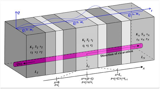
Figure 1.
Three-dimensional (3D) schematic of a tunnel progressively drilled through a subvertical multilayered system: different shades of gray represent different permeability and storability strata (modified after Perrochet et al. []).
In this paper, the key hydrogeological parameters, namely, the hydraulic conductivity K and specific storage coefficient S in Equation (1) are calibrated for optimization. Other parameters ti, Li, si, vi, ri are set as known variables, their values have been specified right after the tunnel division. The measurement of groundwater inflow rate in the tunnel is denoted as Qobs, which are M dimension time series data. In general, M is much larger than N; in other words, the quantity of water inflow measurements is far more than the number of tunnel sectors. Qiobs is referred to as the time series data of the inflow observation in the ith sector, and mi is the number of measured inflows in the ith sector.
The flow chart of dynamic parameter calibration is shown in Figure 2. When the process goes to the ith tunnel sector, the following calculation will be carried out step by step as described below:
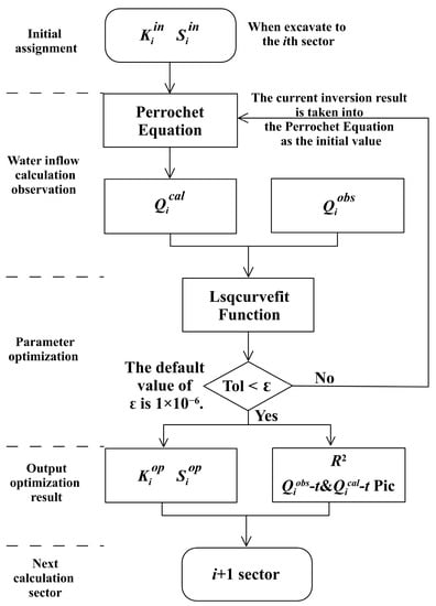
Figure 2.
Flowchart of the dynamic parameter calibration process.
- Initial values assignment: The initial values of Kiin and Siin are assigned to the parameters of hydraulic conductivity and specific storage for sector i.
- Water inflow calculation: This step is denoted as “Perrochet’s Equation” in the flow chart in Figure 2. A MATLAB code script for inflow calculation has been written according to Equation (1). After the initial values of Kiin and Siin are assigned, the code runs, then the inflow calculation is obtained for the ith sector, which is referred to as Qical. It is also a time series including mi values, exactly the same dimension as its paired observation Qiobs.
- Parameter calibration: Once the Qiobs and Qical are available, the trust region reflection algorithm will be applied to calibrate and optimize Ki and Si. The number of iterations in the optimization depends on the stopping condition of the solver, namely, Tolerance, referred to as Tol. When the tolerance is lower than the threshold ε (ε = 1 × 10⁻⁶), the stop criterion is met, then the iteration of the solver will be terminated. In this step, the proposed optimal algorithm will run repeatedly until the stop criterion is met; at that time, the optimized hydraulic conductivity Kiop and specific storage coefficient Siop are determined as well.
- Results output: The optimized Kiop and Siop will be stored in a database to form parameter sets, while the Coefficient of Determination is calculated as:where SSE is the sum of squared errors between observations Qiobs and calculations Qical, and SST stands for the sum of squares. This coefficient is often used to evaluate the fitting effect of optimization. The time-dependent water inflow curves Qiobs-t and Qical-t will be plotted as well, to visually display the fitting effect between calculation and measurement.
- Next calculating sector: As the calibration goes to the (i + 1)th sector, the entire process will be conducted again, as shown in the flowchart in Figure 2. The optimized parameters of the ith sector will be used for water inflow calculation in step (2), and the parameters of the (i + 1)th sector will be calibrated in step (3).
Therefore, the calibration process is carried out dynamically with the tunnel excavation. Thus, the parameters of hydraulic conductivity K and specific storage coefficient S for each sector can be optimized accordingly.
Considering the uncertainties of parameters, we made a slight change to the above dynamic process to realize simultaneous optimization for multiple tunnel sectors. As a result, the same parameters of a sector will be optimized several times. Let k be the number of tunnel sectors in each optimization step, which should be a positive integer greater than or equal to 1. When the calibration process goes to the ith sector, the total k tunnels will be calibrated including the i, i − 1,... i − k + 1 sectors, while the parameters of the i − k to 1 sectors are unchanged, becoming the optimized values by the last calibration. For example, if k = 2, when the process is going to the ith sector, parameters for both the i and i − 1 sectors will be calibrated at this stage, while no parameters will be changed for the i − 2 and all the preceding sectors. In particular, if k = 1, that is, only one sector is being optimized at a time, then the parameters from i − 1 to 1 remain unchanged. Specifically, if i < k, all excavated sectors should be calibrated. For instance, if k = 3, when i = 1 and 2, the first and second sector must be calibrated; when i ≥ 3, there are three sectors to be calibrated in each stage until the final Nth stage. Figure 3 illustrates this example.

Figure 3.
Three-dimensional schematic of the dynamic calibration process when k = 3. Red sectors indicate the parameters being calibrated; Blue sectors indicate that the parameters are fixed or have been calibrated.
It is worth noting that a reference range needs to be set for both hydraulic conductivity K and specific storage coefficient S, which is also the bounded constraint specified in optimization algorithm. Specifically, the optimal value interval of K is set to be 10−10–101 m/d, while it is 10−10–10−1 m−1 for S.
The trust region reflection algorithm was used for parameter calibration in this paper, referred to as TRR, which is a nonlinear least squares optimal algorithm. The basic idea of TRR is to approximate the objective function f(x) with the quadratic function q(s), which is the mapping of the function f(x) on the neighborhood N around the current point x. x is a vector with bounded constraints, and the neighborhood N is called a trust region []. In order to solve the trusted region problem, the test step size s is calculated by minimizing the area N, as shown in Equations (3) and (4). If f(x + s) < f(x), the current point x is updated to x + s. This step is considered a success, and the trust area will continue to the next step. Otherwise, if the step is not successful, then x remains unchanged and the region N will be reduced to the next step [].
where g is the gradient of f(x) for the current x, H is a symmetric matrix of second derivatives, D is a diagonal scaling matrix, ∆ is the trust-region radius > 0, and ‖‖ is the second norm [].
The general process of unconstrained minimization based on the trust region is as follows: Step 1, to construct a two-dimensional trust region subproblem; Step 2, to solve Equation (4) to determine the trial step s; Step 3, if f(x + s) < f(x), then x = x + s; Step 4, to adjust ∆. Repeat these four steps until convergence to obtain the optimized parameter values.
The trust region reflection algorithm can be realized by using the lsqcurvefit function in the MATLAB (R2021b) software.
3. Case Studies
In this section, two case studies of two respective tunnels will be investigated. The transient groundwater inflow for both tunnels were calculated by an analytical model proposed by Perrochet et al. []. In addition, the hydrogeological parameters, namely, the hydraulic conductivity K and specific storage coefficient S, were calibrated by trial-and-error method based on that model. Herein, we will calibrate those parameters by the aforementioned dynamic parameter calibration (DPC) method and compare the results of groundwater inflows and optimized parameter values between the two calibration methods.
3.1. Modane Exploratory Tunnel, France
The Modane exploratory tunnel is located in the French Western Alps and is part of the geologic investigation program of the Lyon–Turin high-speed railway project. This tunnel is excavated in metamorphic rocks belonging to a Permian–Triassic sequence of the so-called “Brianzonese Zone” []. Perrochet et al. [] applied the calculation model of transient water inflow to divide the 760 m tunnel into 10 sectors according to the permeability of the rock stratum based on the collected detailed data. The hydraulic conductivity K and specific storage coefficient S were inverted by the trial-and-error method. The analytical calculation results were in good agreement with the measured values. The application of this approach for tunnel discharge forecasting should therefore always be associated with a reliability analysis of the hydrogeologic conceptual model [].
Here, we applied the dynamic parameter calibration (DPC) to optimize parameters K and S; the tunnel sector division is exactly the same as that in the Reference [], and the parameterization keep same except K and S. The comparison of the time-varying inflow rate between the trial-and-error method and DPC is shown in Figure 4a. The calculated inflow by two methods both presented the dynamic characteristics of the real tunnel inflow. However, the coefficient of determination R2P is 0.9555 by the trial-and-error method in the Reference [], while the R210 is 0.9780 by DPC in this paper (k = 10, all sectors). Because R2P < R210, the fitting effect of DPC is a little better. Figure 4b displays the scatter plots of the measured and calculated inflow.
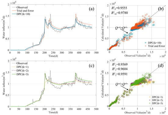
Figure 4.
Comparison between the calculated and observed transient groundwater inflow of the Modane tunnel: (a,c) time series curves; (b,d) scatter diagrams. (Water inflow measurements are from Perrochet et al. []).
DPC can quickly optimize the parameters by computers, and this is a great advantage over the trial-and-error method. Moreover, DPC is stable; no matter what initial values are assigned, the calibration will converge to the same optimized values, indicating that the initial parameter assignment has little effect on the optimization.
In reality, a tunnel is excavated gradually, or the excavation is a dynamic process, so as the excavation progresses forward, the influence of the parameters of the preceding excavated sectors on the inflow calculation for subsequent unexcavated sectors will weaken. Thus, an appropriate k needs to be carefully considered. Here, we set k = 1, k = 2, and k = 3 to calibrate K and S, respectively, instead of the aforementioned k = 10. Figure 4c presents the time-dependent inflow rate for the three cases, and Figure 4d shows the related scatter plots of the measured and calculated values.
The coefficient of determination R2 are 0.9569, 0.9604, and 0.9591 for k = 1, 2, and 3, respectively. Therefore, the result R2P < R21 < R23 < R22 indicates that the fitting effect of DPCs are still slightly better than the trial-and-error method. It also demonstrates that k affects the DPC results; different k will lead to different parameters optimization and different fitting effects as well. Generally, a larger k achieves better fitting; for example, the biggest R2 is 0.9780 when k = 10. However, a larger k also results in more computation and is more time-consuming.
The process of dynamic parameter calibration including nine stages and ten sectors is presented in Figure 5 for the case k = 3. Accordingly, the optimization results of each sector in each stage are presented in Figure 6, wherein the optimized parameters are written as Kij and Sij, where the subscript i represents the ith sector as aforementioned, while the superscript j denotes the jth times optimization for this sector. j should be a positive integer and meets 1 ≤ j ≤ k.
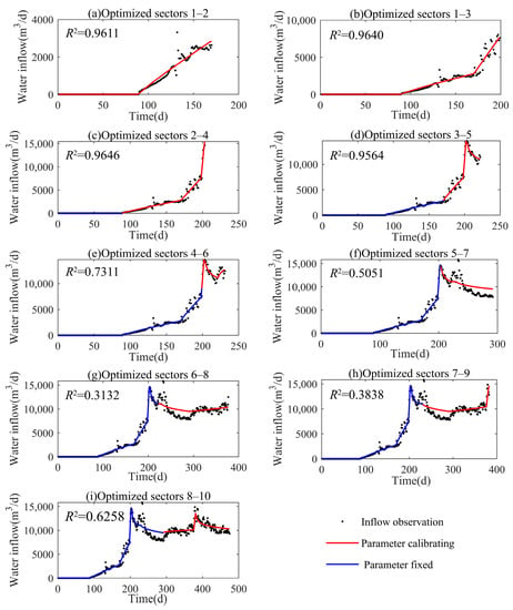
Figure 5.
Comparison between calculated versus measured inflow rate in the process of dynamic parameter calibration (k = 3, R2 is the coefficient of determination of the optimized sectors).
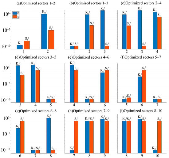
Figure 6.
Optimized parameters of each sector in all 9 steps by DCP (k = 3).
The optimization of the hydraulic conductivity K is relatively stable, namely, the change of K is not significant after several calibrations for the same sector. The range of the K value is 10−3.26–100.99 m/d in the sectors with relatively developed fractures, such as in sectors 2, 3, 4, 6, 8, and 9, as shown in Figure 6. On the other hand, the range is 10−10.00–10−9.76 m/d in the sectors with weak fracture development, as in sections 1, 5, 7, and 10.
The value range of specific storage coefficient S is 10−10.00–10−1.00 m−1. In most sectors, the optimization of S is as stable as K. However, when sectors 2–4 and 3–5 were calibrated, S3 of the 3rd sector changed dramatically, as shown in Figure 6c,d; this may be due to the sudden decrease of the inflow rate in the 5th sector after a steep rise in the 4th sector, seen in Figure 5c,d. Similarly, in Figure 6g,h, the S of the 7th and 8th sectors have increased obviously, in accordance with the significant inflow increase of the 9th sector, as shown in Figure 5g,h.
In Figure 5f–h, when the calibration process goes to sectors 5–7, 6–8, and 7–9, the local coefficient of determination R2 is a little smaller, and the fitting effect of sectors 6 and 7 is not good. Even if the fitting of the 6th sector was greatly improved compared to the 5th sector, it was still not a satisfactory fitting. The water inflow in the 6th sector rose sharply, in order to make a better fit for the subsequent decline sector; the K value in the 6th sector underwent a small decrease after optimization. However, even if the K and S were very small in the 7th sector, its dropping trend still could not be fitted well, as seen in Figure 6e–h. In summary, the abrupt change of inflow brings great difficulty to parameter optimization.
3.2. Xiema Tunnel in Chongqing, China
Xiema Tunnel is located in Beibei District, Chongqing City, Southwest China. The stratum occurring on the entrance side is steep, also the west limb of Guanyinxia Anticline, with an inclination angle of 81~87°. The strata, which the tunnel passes through, successively from new to old include Jurassic Middle Shaximiao Formation (J2s) sandstone with mudstone, Xintiangou Formation (J2x) sandstone with mudstone, Lower Ziliujing Formation (J1zl) sandstone with mudstone, Lower Zhenzhuchong Formation (J1z) sandstone with mudstone, Triassic Upper Xujiahe Formation (T3xj) sandstone shale, Middle Leikoupo Formation (T2l) dolomite limestone, Lower Jialingjiang Formation (T1j) limestone dolomite, and Feixianguan Formation (T1f) limestone with mudstone. The geological cross-section along the tunnel is shown in Figure 7a, and Figure 7b presents the curve of measured inflow versus location. According to the above analysis of the geological conditions of Xiema Tunnel and the geological cross-section, the rock formation in the entrance section of Xiema Tunnel is nearly vertical, which satisfies the prerequisite of using the Perrochet Equation to calculate the water inflow.
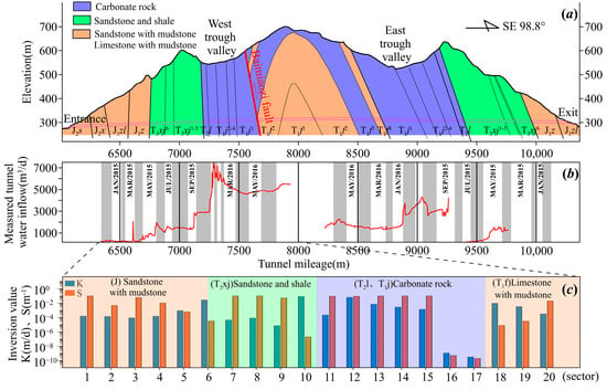
Figure 7.
(a) Transverse geological cross-section of Xiema tunnel; (b) measured groundwater inflow into tunnel during excavation: the dark gray and white color of the tunnel entrance represents the length of the different sectors, totaling 20 sectors; and (c) optimized values of K and S for each sector (Plots (a,b) were modified after Long []).
Perrochet’s analytical equation of transient inflow was used to calibrate the hydraulic conductivity K and specific storage coefficient S of the tunnel rock mass by the trial-and-error method. The results reflect the variation of the time-dependent cumulative inflow of the tunnel []; the coefficient of determination R2X is as high as 0.9284. Here, we calibrated K and S by using the DPC method; with the same tunnel division scheme, the whole 20 sectors were optimized simultaneously, and R220 is 0.9910 larger than R2X. The optimization results are shown in Figure 7c.
The results show that K and S changed significantly when the tunnel passed through the fault impact zone, or near the boundary of two lithologic strata, indicating the change of permeability and storability of the strata accordingly, as shown in sectors 6–7, 10–11 and 17–18 in Figure 7c.
In particular, because the rock stratum in the fault zone and its influence zone is more fractured, the permeability of the rock stratum is generally greater than that of the adjacent rock stratum. In addition, when the tunnel is excavated to the fault zone and its influence zone, the fault zone and its influence zone may have a great influence on the water ingress in the tunnel. This can be seen from the measured water inflow of the tunnel. When the tunnel is excavated to the Baimiaozi fault (the 18th sector), the water inflow increases slightly, as shown in Figure 7b. According to the inversion results, the permeability coefficient of the 18th sector is significantly higher than that of its adjacent sectors 16–17 and 19–20, as shown in Figure 7c. In conclusion, the inversion results of the proposed optimization scheme in the fault zone and its influence zone (occurrence near vertical) are reasonable.
Excluding sectors where the values of K and S largely varied, there are three types of rock mass that can be classified. Type 1: the range of K is 10−4.08–10−2.50 m/d, and S is 10−4.52–10−1.00 m−1 in sectors where sandstone is interbedded with mudstone and limestone with mudstone; Type 2: in sectors where sandstone and shale mainly occur, K is 10−5.16–10−4.11 m/d, and S is 10−1.31–10−1.00 m−1; Type 3: in the carbonate rock strata, K is 10−8.99–10−1.20 m/d, and S is 10−9.31–10−1.00 m−1. Thus, the overall permeability of the rock mass through the tunnel is sequenced as: Type 2 < Type 1 < Type 3; the storability is: Type 1 < Type 2 < Type 3.
In order to evaluate the sensitivities of parameters K and S, we calibrated these two parameters separately. First, parameter K is calibrated, while S is fixed, keeping unchanged. Second, inversely, we calibrate S while K is fixed.
Based on the results of dynamic calibration when k = 3, the probability density function (PDF) and the cumulative distribution function (CDF) are calculated and plotted, respectively. The probability density of both the lgK value and the lgS are approximately bimodal, as seen in Figure 8. When parameter K is fixed, lgS is assigned as −1.0 m−1 in sectors with relative high storability, while lgS is −10.0 m−1 in lower sectors, and lgS is −2.1 m−1 for others. Likewise, when S is fixed, lgK is −1.0 m/d in sectors with greater permeability, while lgK is −10.0 m/d in sectors with lower permeability, and lgK is −3.4 m/d for the rest.
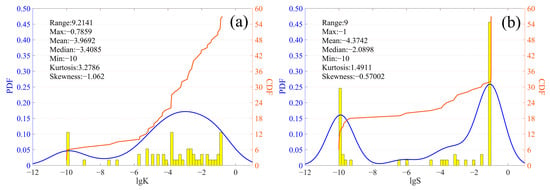
Figure 8.
Probability density, cumulative distribution, and other statistical characteristics of the optimized parameters (k = 3); (a) lgK; (b) lgS.
According to the comparison between these two calibration processes, the fitting effect changed greatly after the 13th sector. Sectors 13–17 were chosen to demonstrate some details; the calculated time-varying water inflow curves are shown in Figure 9 and compared with the measured values.
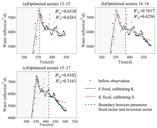
Figure 9.
The comparison between the analytical calculation of the water inflow by DPC against the measured values. (R2K and R2S are the determination coefficients of two calibration processes, respectively. The shadow on the left side of the dashed line indicates the sectors with a fixed parameter, whereas the right side are the sectors with a parameter to be calibrated).
The coefficient of determination R2K by the first way is greater than R2S by the second way, indicating its better fitting effect over the second way, especially in the sectors where water inflow drops sharply as seen in Figure 9. Moreover, the fitting effect of the second way is significantly reduced from sectors 14 to 16, as shown in Figure 9b,c. In Figure 9c, when calibrating sectors 15–17, R2S is rather small by the second way, indicating a poor fitting.
In summary, the fitting effect of the one-parameter calibration by the first way is similar to the two-parameter methods. However, the one-parameter calibration by the second way is greatly different, especially in sectors where water inflow reduces significantly. Therefore, we concluded that the hydraulic conductivity K is more sensitive compared to the specific storage coefficient S, and K has a greater impact on the dynamic calibration.
Although the proposed dynamic calibration methods can optimize parameters effectively, it is worth noting some limitations. Limitation (1): We regarded the water level drawdown s in the Equation (1) as a known condition; however, the groundwater level monitoring data are actually quite lacking in vicinity of a tunnel engineering site. Thus, it may be a key parameter requiring calibration as important as K and S. Limitation (2): When using the optimization scheme, we can set the range of the optimization result first to ensure the rationality of the optimization result, we call this a parameter constraint. The parameter constraint may affect the optimization and fitting, whose effect were not investigated in this paper. These are the problems that need to be further studied and solved in the future. In addition, aside from parameter calibration and estimation, we will further develop some predictive capabilities based on this approach. First, we can evaluate the parameters uncertainty for excavated sectors, and water inflow prediction with parameter uncertainty could be obtained for unexcavated sectors.
4. Conclusions
In this paper, Dynamic Parameter Calibration (DPC) is formed by combining the Perrochet Equation and the Trust Region Reflection (TRR) algorithm, which can quickly obtain the hydrogeological parameters of the constructed sector of the tunnel through the measured water inflow during excavation. The study of two cases proves that this scheme can be used to obtain hydrogeological parameters of tunnels in a subvertical multilayered heterogeneous stratum. The main conclusions are as follows:
- The proposed Dynamic Parameter Calibration (DPC) scheme, which can automatically and quickly optimize hydrogeological parameters by computer, has great advantages over the empirical trial-and-error method. The coefficient of determination R2 by DPC is always greater than that by trial-and-error, which means a better fitting between observation and calculation.
- The number of sectors being calibrated in each step can be set arbitrarily in this DPC scheme. This number has a great influence on the fitting effect, specifically, the more sectors being calibrated, the better the fitting. However, more sectors to be calibrated simultaneously means more parameters to be optimized, and this will lead to massive computation and time consumption. Moreover, the scenario with too many sectors to be optimized simultaneously deviates from the reality of dynamic construction and continuous advancement of tunnel engineering.
- Considering the uncertainty of parameters, the proposed calibration scheme can also conduct multiple optimizations in the same sector. The first case study of the Modane exploration tunnel shows that the hydraulic conductivity K of the same sector is relatively stable after multiple optimizations, and the change is insignificant. The optimization results of the specific storage coefficient S are relatively stable in most sectors, except in the sectors where the inflow changes dramatically.
- For the case where the tunnel passes through heterogeneous strata with different lithologies, the proposed DPC scheme is also applicable. The example of Xiema tunnel demonstrates that K and S will change abruptly near the rock boundary and fault influence zone, reflecting the changes of permeability and storability. The parameter sensitivity analysis shows that K is more sensitive to water inflow than S.
Author Contributions
Data curation, C.C.; Funding acquisition, Q.Z.; Project administration, X.Z. and B.M.; Supervision, Q.X.; Writing—original draft, R.Z.; Writing—review & editing, Q.X. All authors have read and agreed to the published version of the manuscript.
Funding
This research was funded by National Natural Science Foundation of China (42072283, 41502237), Independent project of the State Key Laboratory of Geohazard Prevention and Geoenvironment Protection (SKLGP2017Z014), Open fund for the State Key Laboratory of high-speed Railway Track Technology (2021YJ052), Key Project of Technology Innovation and Application Development of Chongqing, China (cstc2019jscx-dxwtBX0022), and Open project of Chongqing Groundwater Resource Utilization and Environmental Protection Laboratory (MX-3138NC_20191113_104244).
Data Availability Statement
The data used in this study are available from the corresponding author upon request.
Conflicts of Interest
The authors declare no conflict of interest.
References
- Farhadian, H.; Nikvar-Hassani, A. Water flow into tunnels in discontinuous rock: A short critical review of the analytical solution of the art. Bull. Eng. Geol. Environ. 2018, 78, 3833. [Google Scholar] [CrossRef]
- Wu, J.; Zhou, Z.F.; Li, M.W.; Chen, M. Advance on the methods for predicting water inflow into tunnels. J. Eng. Geol. 2019, 27, 890–902. (In Chinese) [Google Scholar]
- Xia, Q.; Xu, M.; Zhang, H.; Zhang, Q.; Xiao, X.X. A Dynamic Modeling Approach to Simulate Groundwater Discharges into a Tunnel from Typical Heterogenous Geological Media during Continuing Excavation. KSCE J. Civ. Eng. 2018, 22, 341–350. [Google Scholar] [CrossRef]
- Perrochet, P. Confined Flow into a Tunnel during Progressive Drilling: An Analytical Solution. Ground Water 2005, 43, 943–946. [Google Scholar] [CrossRef] [PubMed]
- Perrochet, P.; Dematteis, A. Modeling Transient Discharge into a Tunnel Drilled in a Heterogeneous Formation. Ground Water 2007, 45, 786–790. [Google Scholar] [CrossRef] [PubMed]
- Golian, M.; Teshnizi, E.S.; Nakhaei, M. Prediction of water inflow to mechanized tunnels during tunnel-boring-machine advance using numerical simulation. Hydrol. J. 2018, 26, 2827–2851. [Google Scholar] [CrossRef]
- Sun, N.Z. Review of numerical solutions to groundwater inverse problems. Hydrol. Eng. Geol. 1979, 3, 37. (In Chinese) [Google Scholar]
- Zhou, H.Y.; Gómez-Hernández, J.J.; Li, L.P. Inverse methods in hydrogeology: Evolution and recent trends. Adv. Water Resour. 2014, 63, 22–37. [Google Scholar] [CrossRef]
- Poeter, E.P.; Hill, M.C. UCODE, a computer code for universal inverse modeling. Comput. Geosci. 1999, 25, 457–462. [Google Scholar] [CrossRef]
- Xia, Q.; Wan, L.; Wang, X.S.; Poeter, E.P. Principles and applications of the inverse problem program: UCODE. Earth Sci. Front. 2010, 17, 147–151. (In Chinese) [Google Scholar]
- González-Quirós, A.; Comte, J.-C. Hydrogeophysical model calibration and uncertainty analysis via full integration of PEST/PEST++ and COMSOL. Environ. Modell. Softw. 2021, 145, 105183. [Google Scholar] [CrossRef]
- Xu, G.A.; Shao, Y. Three Dimensional Seepage Analysis on Diversion Tunnel of Jinping No.2 Hydropower Station. J. Yangtze River Sci. Res. I 2009, 26, 18–22 + 28. (In Chinese) [Google Scholar]
- Zhang, Q.S.; Li, P.; Wang, G.; Li, S.C.; Zhang, X.; Zhang, Q.Q.; Wang, Q.; Liu, J.G. Parameters Optimization of Curtain Grouting Reinforcement Cycle in Yonglian Tunnel and Its Application. Math. Probl. Eng. 2015, 2015, 615736. [Google Scholar] [CrossRef]
- Xu, Z.H.; Wang, X.T.; Li, S.C.; Gao, B.; Shi, S.S.; Xu, X.J. Parameter Optimization for the Thickness and Hydraulic Conductivity of Tunnel Lining and Grouting Rings. KSCE J. Civ. Eng. 2019, 23, 2772–2783. [Google Scholar] [CrossRef]
- Ma, C.J.; Jiang, A.N.; Wang, J.X.; Chen, W.; Hu, X.F.; Liu, Y.H. Intelligent back analysis of Tunnel seepage based on differential evolution algorithm and its engineering application. J. Railw. Sci. Eng. 2016, 13, 898–905. (In Chinese) [Google Scholar]
- Chen, S.; Dong, S.N. A Sequential Structure for Water Inflow Forecasting in Coal Mines Integrating Feature Selection and Multi-Objective Optimization. IEEE Access 2020, 8, 183619–183632. [Google Scholar] [CrossRef]
- Zhou, L.; Yang, G.Q.; Yang, Q.C. Prediction of water inflow in karst tunnels based on optimal combination model and rescaled range method. Eng. J. Wuhan Univ. 2020, 53, 875–882. (In Chinese) [Google Scholar]
- Coli, M.; Pinzani, A. Tunnelling and Hydrogeological Issues: A Short Review of the Current State of the Art. Rock Mech. Rock Eng. 2014, 47, 839–851. [Google Scholar] [CrossRef]
- Tomasz, K.; Joanna, N.; Aleksandra, N.-L.; Tomasz, B.; Grzegorz, K. Analysis of the interaction between surface water and groundwater using gaseous tracers in a dynamic test at a riverbank filtration intake. Hydro Pro. 2023, 37, e14862. [Google Scholar] [CrossRef]
- Liu, S.; She, D.X.; Zhang, L.P.; Ding, K.X.; Guo, M.Y.; Chen, L. Parameter sensitivity analysis of hydrological model based on Morris and Sobol. Resour. Environ. Yangtze Basin 2019, 28, 1296–1303. (In Chinese) [Google Scholar]
- Cesano, D.; Olofsson, B.; Bagtzoglou, A.C. Parameters Regulating Groundwater Inflows into Hard Rock Tunnels—A Statistical Study of the Bolmen Tunnel in Southern Sweden. Tunn. Undergr. Space Technol. 2000, 15, 153–165. [Google Scholar] [CrossRef]
- Holmøy, K.H.; Nilsen, B. Significance of Geological Parameters for Predicting Water Inflow in Hard Rock Tunnels. Rock Mech. Rock Eng. 2014, 47, 853–868. [Google Scholar] [CrossRef]
- Jiang, X.N.; Zhang, W.; Cheng, D.H.; Yang, Y.K.; Liu, C.; Cai, W.S.; Qiao, X.Y. Estimation of mine water inflow using the partially penetrated virtual large-diameter well method and partially horizontal collector gallery method. J. Water Resour. Water Eng. 2018, 29, 169–174. (In Chinese) [Google Scholar]
- Tang, Y.C.; Zhang, J.M.; Li, L.X. Calculation method of water inflow in pumping well based on wavelet neural network replacement model. Water Res. Power. 2020, 38, 17–20 + 70. (In Chinese) [Google Scholar]
- Le, T.M.; Fatahi, B. Trust-region reflective optimisation to obtain soil visco-plastic properties. Eng. Comput. 2016, 33, 410–442. [Google Scholar] [CrossRef]
- Long, K. Analytical Solution of Transient Discharge into the Xiema Tunnel of Zhongliang Mountain in Chongqing. Chin. J. Undergr. Space Eng. 2016, 12, 815–820. (In Chinese) [Google Scholar]
Disclaimer/Publisher’s Note: The statements, opinions and data contained in all publications are solely those of the individual author(s) and contributor(s) and not of MDPI and/or the editor(s). MDPI and/or the editor(s) disclaim responsibility for any injury to people or property resulting from any ideas, methods, instructions or products referred to in the content. |
© 2023 by the authors. Licensee MDPI, Basel, Switzerland. This article is an open access article distributed under the terms and conditions of the Creative Commons Attribution (CC BY) license (https://creativecommons.org/licenses/by/4.0/).