Article

Research and Application of the Calculation Method of River Roughness Coefficient with Vegetation

1
Key Laboratory of Changjiang Regulation and Protection of Ministry of Water Resources, Changjiang Survey, Planning, Design and Research Co., Ltd., Wuhan 430010, China
2
Changjiang River Scientific Research Institute of Changjiang Water Resources Commission, Wuhan 430010, China
*
Author to whom correspondence should be addressed.
Water 2023, 15(14), 2638; https://doi.org/10.3390/w15142638
Submission received: 8 June 2023 / Revised: 11 July 2023 / Accepted: 14 July 2023 / Published: 20 July 2023
(This article belongs to the Special Issue Vegetation-Influenced Water Flow and Sediment Transport)

Abstract

:
The roughness coefficient is a comprehensive parameter reflecting river resistance, which is widely used in the planning and design of river regulation and flood control projects. In recent years, as the upstream water conservancy and hydro-power projects have been put into operation, the frequency of low flow in the middle and lower reaches has increased, and the frequency of flood flow has decreased. All kinds of vegetation in the river floodplain grow luxuriantly, which causes a change in the river resistance and roughness coefficient. The present study was carried out with theoretical analysis and laboratory tests. A formula for the roughness coefficient calculation was derived based on the momentum equilibrium equation and momentum exchange between the vegetation layer and upper layer. The relationship between the depth-averaged velocity within the vegetation layer and depth-averaged velocity of the whole flow was analyzed. The reliability of the formula was verified by a large amount of previous experimental data. Based on the derived formula, the variation law of the roughness coefficient with vegetation density, vegetation height, and water depth were obtained. For the emerged vegetation flow, the Manning coefficient tended to increase with the increase in the vegetation density and water depth. For the submerged vegetation flow, the Manning coefficient showed a trend of decreasing with the increase in the water depth and increased with the increase in the vegetation height. Finally, the derived formula was applied in the Yueyang reach of the Yangtze River and the Duliujian River. The study can be applied in the fields of water level-flow discharge relationship analysis and the water surface line calculation of vegetated rivers.

1. Introduction

Aquatic vegetation is widely found in rivers, wetlands, and coasts. It has the functions of protecting banks, improving the water quality, and maintaining ecosystem diversity. Costanza et al. [1] estimated that the value of ecological services, which include providing nutrients and habitat, controlling erosion, protecting banks, etc., provided by aquatic vegetation was as high as USD 10 trillion per year. Aquatic vegetation is also widely used in river regulation and management. Due to the extensive engineering applications and important ecological functions of aquatic vegetation, studies related to it have received widespread attention in recent years [2,3,4] and have gradually developed into the field of vegetation hydraulics.
Vegetation resistance has become a key field of vegetation hydraulics research because of its importance in modifying flow velocity. Typically, studies of vegetation resistance focus on the Manning coefficient n, friction coefficient f, or shear stress of vegetation flow [5,6,7]. In the early stage, researchers established the relationship between the Manning coefficient n and averaged velocity U and hydraulic radius R by field observations or laboratory experiments [8]. Kouwen et al. [9] introduced the stiffness parameter MEI to the relationship, and MEI reflected the effect of vegetation deformation on the roughness coefficient. The U.S. Soil Conservation Service (SCS) has developed tables of roughness coefficients corresponding to various types of vegetated channels to facilitate engineering applications. Some researchers have used the friction coefficient f to describe vegetation resistance. Kouwen and Unny [10], based on flume tests, inferred that the friction coefficient f caused by flexible plastic sheets was related to the relative roughness and oscillation mechanism of plastic sheets. Jarvela [11] obtained the Darcy–Weisbach coefficient f as a function of Reynolds number, flow velocity, water depth, and relative roughness based on flume tests with grass and willow. As measurement techniques advanced, researchers gradually investigated vegetation resistance through systematic model tests. For nearly rigid vegetation such as willow and reed, the vegetation was simplified as a cylindrical or strip shape. Based on the quadratic relationship between the resistance and flow velocity, the variation in the resistance coefficient with flow velocity and vegetation density was analyzed. Stone and Shen [12] used the maximum flow velocity between vegetation as the characteristic velocity. The drag coefficient did not change with the vegetation volume fraction, vegetation diameter, and vegetation Reynolds number when using the averaged velocity within vegetation as the characteristic velocity drag coefficient increased with the increase in the vegetation volume fraction and decreased with the increase in vegetation Reynolds number. Tanino and Nepf [13] conducted a detailed experimental study on the drag coefficient of randomly arranged rigid vegetation and obtained the relationship between the coefficient CD and vegetation Reynolds number and vegetation volume fraction. Yang and Choi [14] calculated the depth-averaged velocity based on solving the velocity distribution in the vegetation layer and the layer above the vegetation, and then obtained the Manning coefficient with vegetation according to the Manning formula. They proposed a coefficient Cu in the velocity distribution of the layer above the vegetation, and Cu = 1 for a ≤5.0 m−1, Cu = 2 for a >5.0 m−1. Cu was found to vary significantly among different vegetation, which caused a large deviation from the predicted Manning coefficient. Li S et al. [15] divided the vegetated flow into the suspension layer and basal layer, based on which the averaged velocity over the whole flow depth could be derived, and then the Manning coefficient was derived from the Manning formula. They introduced the representative length scale h* into the calculation, which was calculated with energy slope. However, the energy slope is very difficult to obtain in practice. Cheng [16] proposed a representative roughness height to quantify the effect of submerged vegetation on flow resistance in the surface layer, and then developed an approach to estimate the average flow velocity and resistance coefficients for both cases of rigid and flexible vegetation, which was also the calculation of the energy slope. Overall, the methods calculating the Manning coefficient proposed by previous researchers are relatively complicated and need many calculation parameters, especially the energy slope, which is difficult to obtain. Because the research object and derivation process of each method is different, the validation data used are also different, so the resistance coefficients predicted by each method also differ. Wang et al. [17] found that the resistance coefficients of the emerged vegetation calculated by different methods were basically the same, but the calculated resistance coefficients of inundated vegetation varied greatly, and the differences among the results of different methods could be up to 2~4 times.
In flood level prediction and river evolution simulation for rivers containing vegetation, the influence of vegetation is often considered by increasing the resistance. A careful examination and choice of the roughness coefficient is essential. Large deviations in the prediction of vegetation resistance would bring large errors to the aforementioned computational simulations, which would in turn affect the practice of river regulation. For example, the Hec-RAS model result was more accurate when the resistance coefficient was calculated dynamically using the characteristic vegetation [17]. Therefore, how to calculate the roughness coefficient of the river containing vegetation easily and scientifically is an importance issue that needs to be solved. In this paper, based on theoretical analysis and data validation, a relatively convenient and accurate method for calculating the Manning coefficient with vegetation is proposed.

2. Methods and Materials

2.1. Calculation Method of Roughness Coefficient with Vegetation

The vegetation-induced drag FD can be described by using the drag coefficient CD.
F D = 1 2 C D a U 1 2
where FD is the vegetation resistance per unit mass of fluid; CD is the vegetation drag coefficient; a is the vegetation density defined by the projected area in the incoming flow plane per unit volume; a = N × d; N is the number of vegetation per unit area; d is the vegetation characteristic length, for cylindrical vegetation, the characteristic length can be used with diameter; U1 is the mean velocity in the vegetated layer. According to previous research [6,7], the vegetation resistance coefficient varies with the vegetation Reynolds number, vegetation density, etc. For low vegetation density, the drag coefficient CD is generally taken as 1.0.
Assuming the vegetation flow is constant and uniform, and the vegetation resistance, bed resistance, and gravity are balanced along the direction of flow, the equation for force balance with submerged vegetation (see Figure 1) is
1 2 C D a h U 1 2 + 1 8 f ( 1 ϕ ) U 2 = H g S 0 ( 1 ϕ )
where U is the depth-averaged velocity over the whole flow depth and U1 is the depth-averaged velocity within the vegetation layer. When vegetation is submerged, U1 < U, when vegetation is emerged, U1 = U; a is the vegetation density; h is the vegetation height below the water surface; H is the water depth when the vegetation is emerged, h = H; g is the acceleration of gravity; f is the Darcy–Weisbach coefficient; S0 is the water surface slope; CD is the vegetation drag coefficient; Φ is the vegetation volume fraction; for cylindrical vegetation, Φ equals adπ/4 and d is the vegetation diameter.
The water surface slope S0 and Darcy–Weisbach coefficient f can be calculated from the following equation,
U = 1 n R 2 3 S 0 1 2
f = 8 g / C 2
C = R 1 / 6 / n 0
where n is the Manning coefficient of the river with vegetation and R is the hydraulic radius. Generally, the river width is much larger than the water depth, so the hydraulic radius can be expressed by the mean water depth H; C is the Chezy coefficient; n0 is the roughness coefficient without vegetation.
Combining Equation (2) with Equation (3) to Equation (5), the Manning coefficient n with vegetation was obtained as
n = 1 2 C D a h H 1 3 ( U 1 U ) 2 g ( 1 ϕ ) + n 0 2
When the vegetation is emerged, U1 = U, and the Manning coefficient, Equation (6), with vegetation can be simplified as
n = 1 2 C D a h H 1 3 g ( 1 ϕ ) + n 0 2
When the vegetation is submerged, the vegetation flow can be divided into two-layer models. The relationship between U1 and U can be expressed as follows (see Chen et al. [18]).
U 1 U = 1 1 h H ϕ + C D a h 2 C ( 1 ϕ ) ( H h H ) 3
The coefficient C describes the efficiency of momentum exchange between the vegetation layer and non-vegetation layer. C can be considered as a constant, taking the value of 0.009. Substituting Equation (8) into Equation (7), the Manning coefficient with submerged vegetation flow can be expressed as
n = 1 2 C D a h H 1 3 ( 1 / ( 1 h H φ + C D a h 2 C ( 1 φ ) ( H h H ) 3 ) ) 2 g ( 1 ϕ ) + n 0 2

2.2. Materials

Previous researchers have conducted many experiments (see Table 1) including Shimizu et al. [19], Dunn et al. [20], Meijer and van Velzen [21], Lopez and Garcia [22], Ghisalberti and Nepf [23], Murphy et al. [24], Nezu and Sanjou [25], Yan [26], Yang [27], and Cheng [16]. With these experiments, the calculation method can be validated.
The main experimental parameters of the above-mentioned researchers were as follows. The test flume width ranged from 0.3 m to 3.0 m, water depth ranged from 0.05 m to 2.5 m, energy slope ranged from 0.018‰ to 16‰, flow velocity ranged from 0.01 m/s to 1.24 m/s, vegetation height ranged from 0.035 m to 1.5 m, vegetation diameter ranged from 0.001 m to 0.008 m, vegetation density ranged from 0.27 m−1 to 29 m−1, and the vegetation volume fraction ranged from 0.14% to 11.9%. n0 was determined by the corresponding test results, and where the model test was not given, it was generally taken as 0.011.

3. Results

3.1. Model Validation

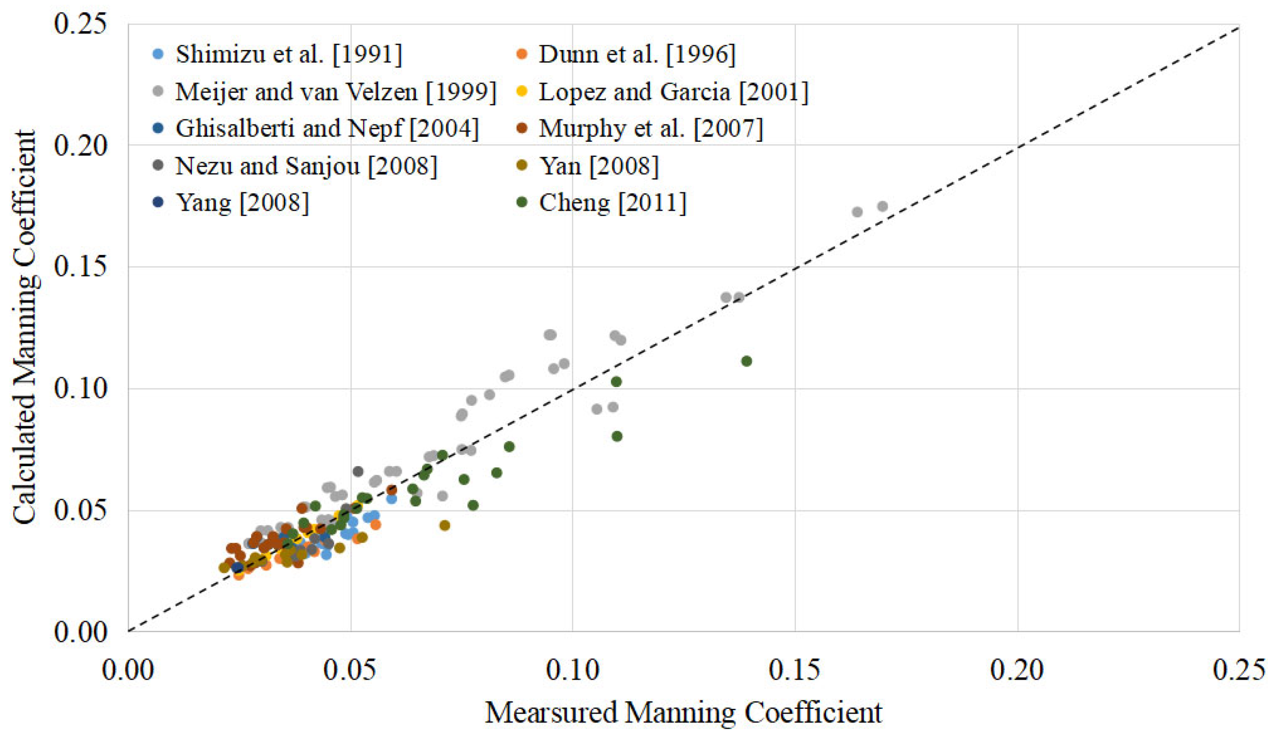
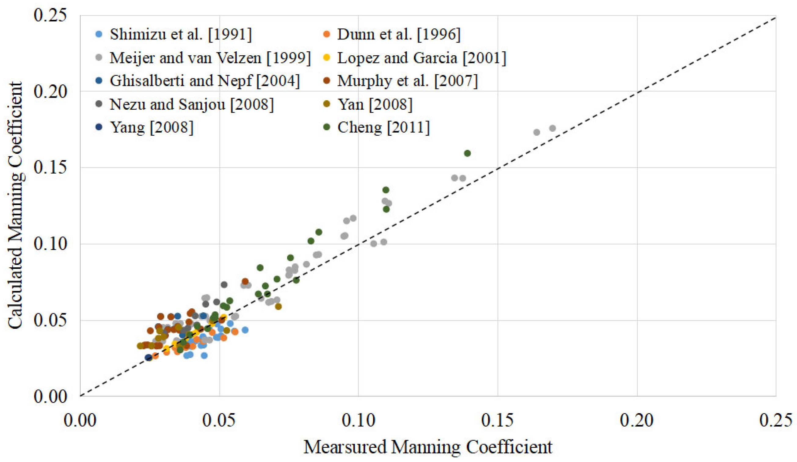
The comparison with the calculated Manning coefficient using Equation (9) with the measured Manning coefficient in each test is shown in Figure 2. The validation results showed that the Manning roughness calculated by Equation (9) did not differ much from the measured coefficient, with a standard deviation of 17.5%. The comparisons with the calculated Manning coefficient using Yang and Choi’s equation [8] and Li et al.’s [9] equation with the measured Manning coefficient in each test are shown in Figure 3 and Figure 4. The R-square of Equation (9) was 0.88, the R-square of Yang and Choi’s equation was −10.83, and R-square of Li et al.’s equation was 0.85. It can be seen that the model accuracy of Equation (9) was much better than Yang and Choi’s equation and comparable to that of Li et al. Considering that Equation (9) involves the parameters of the natural property of the river and vegetation, it does not utilize the water surface slope, which is commonly used by other researchers [14,15] but is difficult to obtain. We believe that the practical value of Equation (9) would be higher than the common formula for calculating the roughness coefficient with vegetation.

3.2. Variation of Roughness Coefficient

In this section, Equations (6) and (9), derived in the previous section, were used to analyze the effects of variation in the vegetation density, vegetation height, and water depth on the Manning coefficient of natural river floodplains. Natural river floodplains consist of trees and shrubs, reeds, etc., which present an emerged or submerged state when the river is in a flood stage.
(1)
Emerged vegetation flow
Trees, which are used to protect embankments, are commonly planted in the floodplain. According to the field survey of the Jingjiang River of the Yangtze River, the averaged tree diameter is about 0.1 m, and the density a is generally between 0.01 and 0.2 m−1. Based on the experience and the hydraulic calculation manual, the Manning coefficient n of the floodplain without vegetation was taken as 0.03. According to Equation (7), the variation of the Manning coefficient n with the vegetation density and floodplain water depth is shown in Figure 5. It can be seen that for emerged vegetation, the Manning coefficient tends to increase with the increase in the vegetation density and floodplain water depth. The Manning coefficient was about 0.032 for a floodplain water depth of 0.5 m and vegetation density of 0.01 m−1, 0.071 for a floodplain water depth of 0.5 m and vegetation density of 0.2 m−1, 0.056 for a floodplain water depth of 3 m and vegetation density of 0.01 m−1, and 0.214 for a floodplain water depth of 3 m and vegetation density of 0.2 m−1.
(2)
Submerged vegetation flow
Flexible vegetation such as weeds, crops, and low shrubs are also found in the floodplain. This kind of vegetation bends with the current under the action of water flow and is often in the submerged state. Combined with the relevant literature and field survey, the density of weeds and other flexible vegetation in the floodplain is generally 0.2~5 m−1. When vegetation is in the submerged state, the height h of vegetation below the water surface is the effective height after bending under the action of water flow. According to Equation (9), the relationship of the Manning coefficient with vegetation density, floodplain water depth, and vegetation height is shown in Figure 6 and Figure 7. Under the same vegetation height condition, the greater the water depth, the smaller the Manning coefficient, and the greater the vegetation density, the larger the Manning coefficient; the Manning coefficient increases with the increase in the vegetation density and decreases with the increase in the floodplain water depth. Under the same condition of vegetation height h = 0.5 m, the Manning coefficient was 0.050 when the water depth was 1 m and the vegetation density was 0.2 m−1, 0.097 when the water depth was 1 m and the vegetation density was 5 m−1, 0.043 when the water depth was 3 m and the vegetation density was 0.2 m−1, and 0.063 when the water depth was 1 m and the vegetation density was 5 m−1.
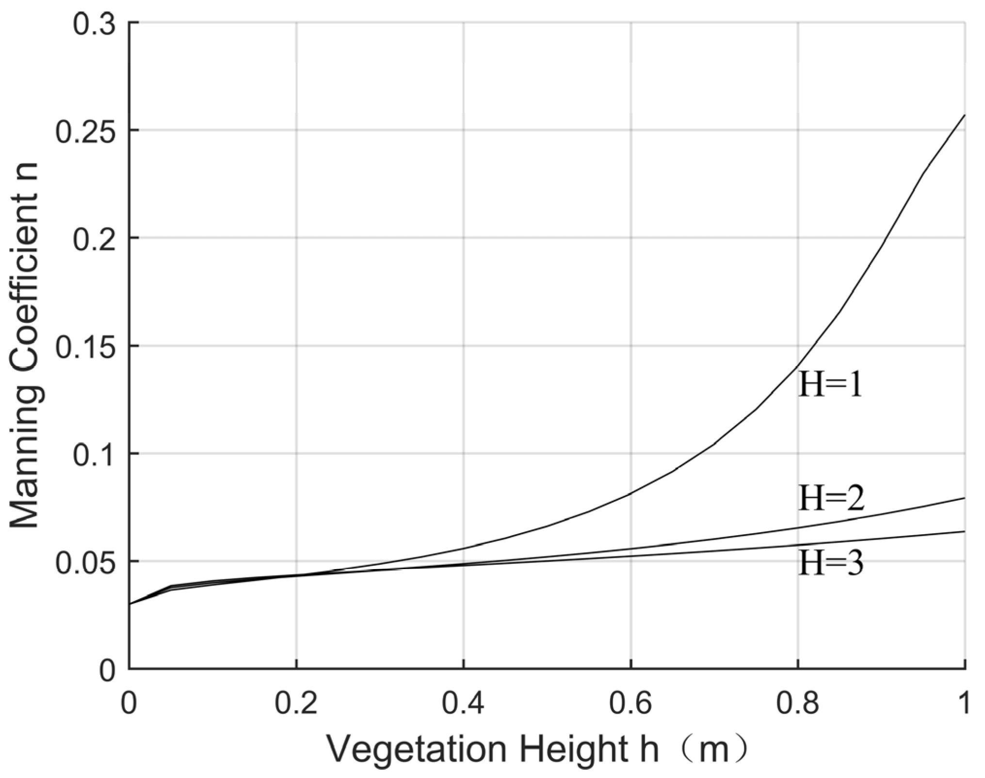
Under the same vegetation density condition, the Manning coefficient also showed a phenomenon of decreasing with increasing water depth and increasing with vegetation height. Under the condition that the vegetation density is constant (a = 1.0 m−1), the Manning coefficient increased from 0.03 to 0.257 during the increase in vegetation height from 0 to 1.0 m at a floodplain water depth of 1.0 m, and from 0.03 to 0.064 during the increase in vegetation height from 0 to 1.0 at a vegetation water depth of 3.0 m.
The above analysis shows that the Manning coefficient increases significantly when vegetation is present on the floodplain. The Manning coefficient of vegetation generally varies between 0.03 and 0.2. The Manning coefficient of low and sparse vegetation is smaller, while the Manning coefficient of tall and dense vegetation is larger. The above variation pattern can be explained by the vegetation water retention mechanism. The main reason for vegetation water blockage is that the water flow produces vortices of different scales under the action of vegetation including vortices formed by vegetation branches and leaves, and shear vortices formed by submerged vegetation tops. Vortices of different sizes dissipate part of the kinetic energy of the water flow into internal energy, which leads to the slowing down of the water flow and the formation of the water blocking effect. For non-submerged vegetation, the greater the water depth, the more vortices are produced by vegetation, so the greater the energy lost, and the greater the force of vegetation on water flow; the greater the density of the vegetation, the same principle applies, resulting in the phenomenon of increasing the water depth or vegetation density and increasing the Manning coefficient. For submerged vegetation, the water depth of the floodplain increases, therefore the flow velocity of the vegetation layer will decrease, the vortex generated by the vegetation layer decreases, and the energy lost decreases, resulting in the phenomenon of an increase in the water depth and a decrease in the stratification coefficient.

4. Practical Applications

In this section, we applied the roughness calculation method to two typical river sections in the Yangtze and Haihe Basins to illustrate the practicality of the method.

4.1. Emerged Vegetation Flow

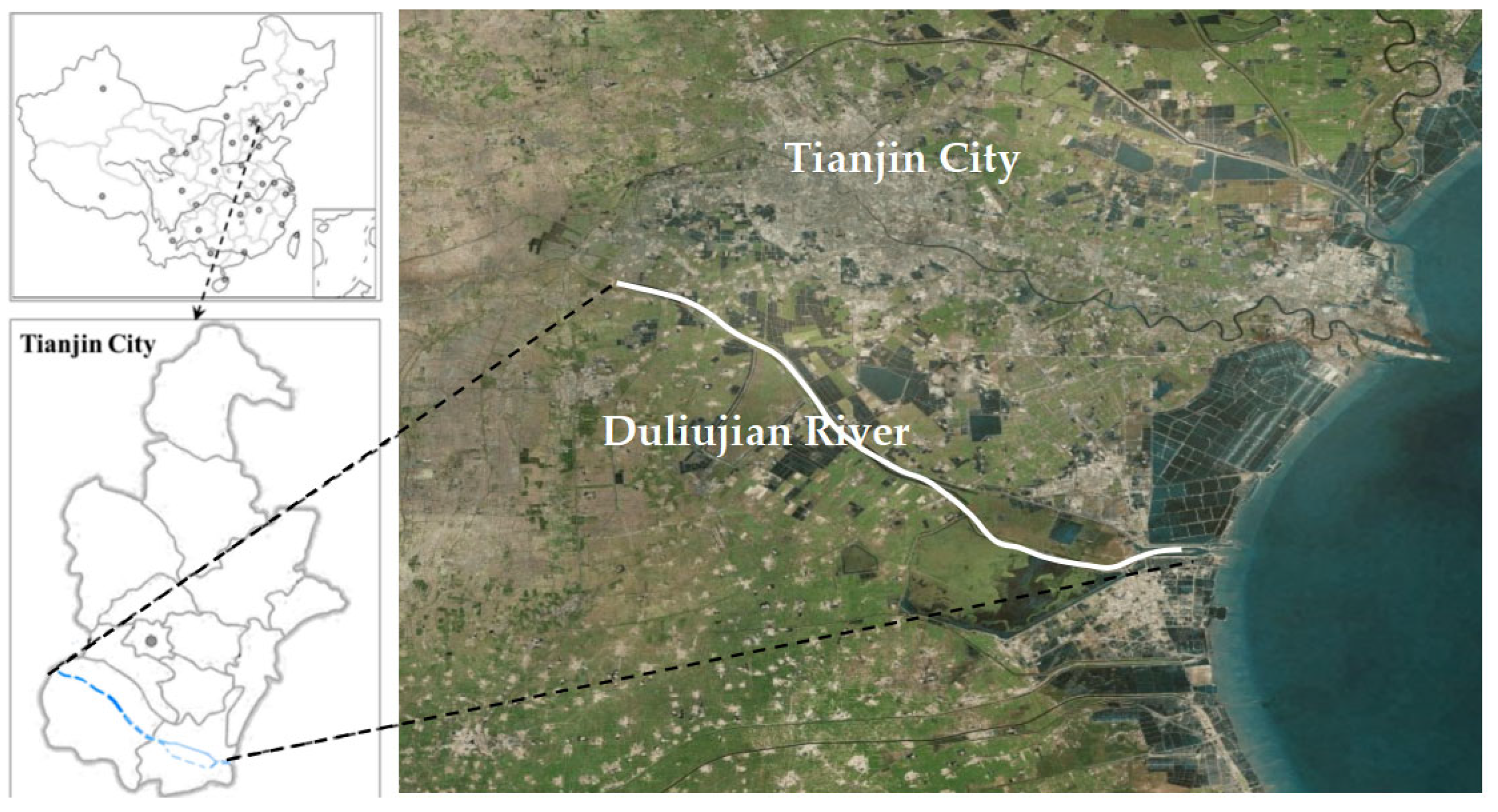
The Duliujian River is an important flood passage of Tianjin. The research subject is a typical reach of the upper Duliujian River (see Figure 8). Trees are the typical vegetation of the river reach. The average diameter of trees is 6 cm, the number of trees per unit area is 0.18, the height of trees is 10 m, and the density of trees is 0.011 m−1. The averaged elevation of the river floodplain is about 2.5 m, and the one hundred-year flood level is 5.73 m. During the one hundred-year flood, the averaged depth of floodplain is 3.23 m, and the trees are in an emerged state. The floodplain roughness coefficient without vegetation was taken as 0.025 (the parameters above can be found in Gao et al. [28]). According to Equation (7), the roughness coefficient of the river with trees is 0.057. This result is basically consistent with the roughness coefficient of 0.06 (see Gao et al. [28]) derived from the experiment.

4.2. Submerged Vegetation Flow

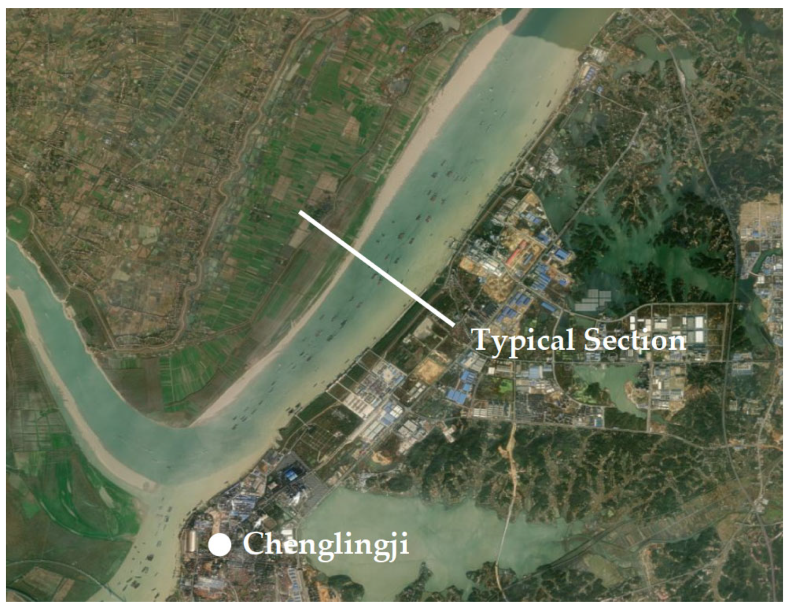
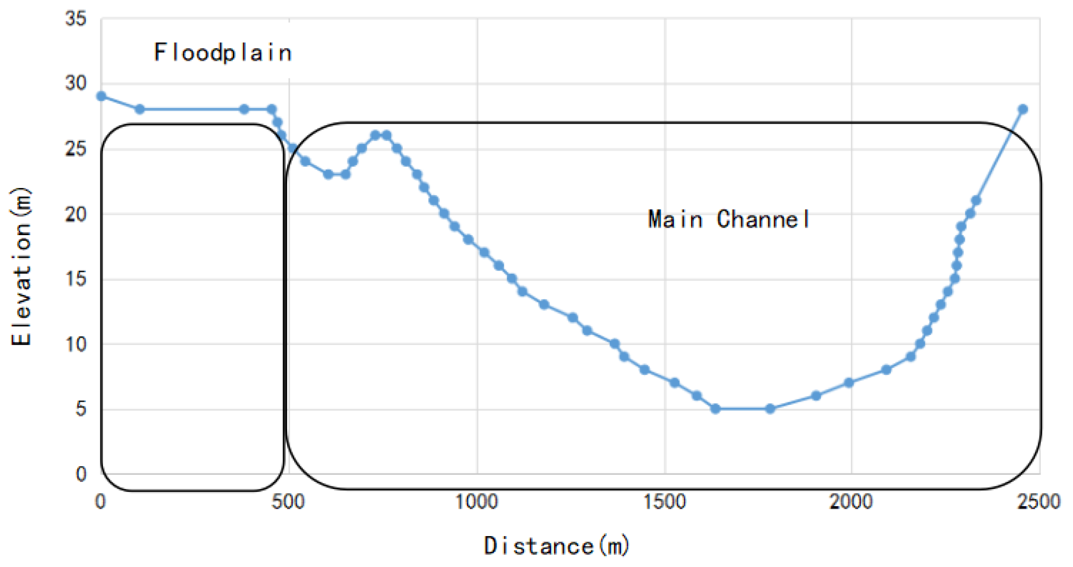
The middle reaches of the Yangtze River (see Figure 9) are a key area for flood control, and there is much vegetation on the river floodplain. The Yueyang River section is located below the confluence of the Jing River and Dongting Lake, which faces a serious flood control situation in the middle reaches of the Yangtze River. Therefore, the Yueyang River reach was chosen as the study site. This river reach is a compound channel. The width of the river is about 2500 m, the width of the left floodplain is about 400–500 m, and the width of the right floodplain is less than 100 m. Shrubs and crops predominate on the floodplain.
The average diameter of vegetation is about 1 cm, the number of vegetation per unit area is 200 plants/m2, the height of vegetation is 50 cm, and the density of vegetation is 2 m−1. The averaged elevation of the floodplain is about 28 m, and the design flood level of this reach is 32.36 m. Under the design flood level, the average water depth of the floodplain is about 4.36 m. The height of vegetation after bending is 0.4 m under the design flood conditions. According to Equation (9), the Manning coefficient of the floodplain is 0.057. Due to the completion and operation of the Three Gorges Project, the chances of flooding in the river reach downstream of the Three Gorges have been significantly reduced. The vegetation coverage on the floodplain has increased compared with its status before the Three Gorges Project, in particular, the density of shrubs and other flexible vegetation has increased significantly. Assuming that the vegetation density before the completion of the Three Gorges was 1 m−1, other parameters of the vegetation remained unchanged. According to Equation (9), the Manning coefficient of the floodplain is 0.054. Therefore, when the vegetation density increases from 1 m−1 to 2 m−1, the Manning coefficient of the floodplain increases from 0.054 to 0.057, which is an increase of about 5.5%.
Next, the authors analyzed the effect of changes in floodplain resistance on river resistance. A typical cross-section was chosen, as shown in Figure 10 and Figure 11.
Based on the channel river integrated roughness coefficient (i.e., the Manning coefficient) calculation method:
n = ( P 1 i = 1 i = N P i n i 3 / 2 ) 2 / 3
where Pi, ni are the wetted perimeter and the Manning coefficient of the ith segmented section, respectively. The typical section of Figure 10 can be divided into two zones, namely, the main channel zone and the floodplain zone. The wetted perimeter of the floodplain and the main channel was 450 m and 2007 m, respectively. Combined with the results of the previous analysis, the Manning coefficients of the floodplain before and after the change in the vegetation density were 0.054 and 0.057, respectively; the Manning coefficient of the main channel remained unchanged at 0.025. The integrated roughness of the section before and after the change in vegetation density was 0.0303 and 0.0309, respectively. The integrated roughness of the section increased after an increase in the vegetation density by about 2.0%.
The above study shows that computational parameters of this method are easy to obtain, and the computational process is simple. The method has achieved good results in the water flow of trees, shrubs, and other vegetation. We can see that the calculation method is mainly established based on rigid or near-rigid vegetation, and the momentum exchange coefficient between the vegetation and non-vegetation layers can also be determined based on rigid or near-rigid vegetation. Therefore, we believe that the model proposed in this paper should be mainly used for vegetation such as trees, reeds, and shrubs as the method application may have large errors for flexible vegetation with large deformation under the action of water flow; in cases where there are more leaves or vegetation, density a is difficult to assess accurately.

5. Conclusions

In this paper, the calculation method of the Manning coefficient was derived based on the momentum equilibrium equation and momentum exchange between the vegetation layer and upper layer. The Manning coefficient is primarily related to the vegetation characteristics and water depth. The variation law of floodplain roughness with vegetation density, vegetation height, and water depth was explored. The study showed that for emerged vegetation, the Manning coefficient tends to increase with the increase in the vegetation density and floodplain water depth. For submerged vegetation, the Manning coefficient showed a trend of decreasing with the increase in the water depth and increasing with the increase in the vegetation height. The Manning coefficient for vegetated flow generally ranges from 0.03 to 0.2. The application of Equation (9) in the Yueyang River section of the middle and lower reaches of the Yangtze River showed that the increase in vegetation density after the Three Gorges Project led to an increase in the floodplain Manning coefficient, which increased from 0.054 to 0.057, an increase of about 5.5%, and the comprehensive Manning coefficient of a typical section increased from 0.0303 to 0.0309, an increase of about 2.0%. The results of the study can be applied in the analysis of the water level-flow relationship and water surface line calculation of a vegetated river. It is important to note that further research is needed as to whether the present method is applicable to flexibly submerged vegetation with large deformations.

Author Contributions

Conceptualization, Z.C. and Q.C.; Methodology, Z.C. and J.Z.; Validation, Z.C. and J.Z.; Formal analysis, Z.C.; Investigation, Z.C.; Writing—original draft preparation, Z.C., J.Z. and Q.C.; Writing—review and editing, Z.C. All authors have read and agreed to the published version of the manuscript.

Funding

This research was funded by the National Natural Science Foundation of China (No. U2040216) and Fundamental Research Funds for Central Public Welfare Research Institutes (CKSF2021439/HL).

Data Availability Statement

The data used in this study can be obtained from the references mentioned in the text.

Conflicts of Interest

The authors declare no conflict of interest.

References

  1. Costanza, R.; d’Arge, R.; de Groot, R.; Farber, S.; Grasso, M.; Hannon, B.; Limburg, K.; Naeem, S.; O’Neill, R.V.; Paruelo, J.; et al. The value of the world’s ecosystem services and natural capital. Nature 1997, 387, 253–260. [Google Scholar] [CrossRef]
  2. Nepf Heidi, M. Flow and Transport in Regions with Aquatic Vegetation. Annu. Rev. Fluid Mech. 2012, 44, 123–142. [Google Scholar] [CrossRef] [Green Version]
  3. Liu, C.; Shan, Y. Impact of an emergent model vegetation patch on flow adjustment and velocity. Proc. Inst. Civ. Eng.-Water Manag. 2022, 175, 55–66. [Google Scholar] [CrossRef]
  4. Liu, C.; Yan, C.; Sun, S.; Lei, J.; Nepf, H.; Shan, Y. Velocity, turbulence, and sediment deposition in a channel partially filled with a Phragmites australis canopy. Water Resour. Res. 2022, 58, e2022WR032381. [Google Scholar] [CrossRef]
  5. Nicosia, A.; Ferro, V. Flow resistance due to shrubs and woody vegetation. Flow Meas. Instrum. 2023, 89, 102308. [Google Scholar] [CrossRef]
  6. Lauria, A. Flow Resistance in Open Channel due to Vegetation at Reach Scale: A Review. Water 2021, 13, 116. [Google Scholar]
  7. Ikhsan, C.; Permana, A.S.; Negara, A.S. Armor layer uniformity and thickness in stationary conditions with steady uniform flow. Civ. Eng. J. 2022, 8, 1086–1099. [Google Scholar] [CrossRef]
  8. Ree, W. Hydraulic characteristics of vegetation for vegetated waterways. Agric. Eng. 1949, 30, 184–189. [Google Scholar]
  9. Kouwen, N.; Unny, T.; Hill, H.M. Flow retardance in vegetated channels. J. Hydraul. Div. ASCE 1969, 95, 329–342. [Google Scholar] [CrossRef]
  10. Kouwen, N.; Unny, T.E. Flexible roughness in open channels. J. Hydraul. Div. ASCE 1973, 99, 713–728. [Google Scholar] [CrossRef]
  11. Järvelä, J. Flow resistance of flexible and stiff vegetation: A flume study with natural plants. J. Hydrol. 2002, 269, 44–54. [Google Scholar] [CrossRef]
  12. Stone, B.M.; Shen, H.T. Hydraulic resistance of flow in channels with cylindrical roughness. J. Hydraul. Eng. 2002, 128, 500–506. [Google Scholar] [CrossRef]
  13. Tanino, Y.; Nepf, H.M. Laboratory investigation of mean drag in a random array of rigid, emergent cylinders. J. Hydraul. Eng. 2008, 134, 34–41. [Google Scholar] [CrossRef]
  14. Yang, W.; Choi, S. A two-layer approach for depth-limited open-channel flows with submerged vegetation. J. Hydraul. Res. 2010, 48, 466–475. [Google Scholar] [CrossRef]
  15. Li, S.; Shi, H.; Xiong, Z.; Huai, W.; Cheng, N. New formulation for the effective relative roughness height of open channel flows with submerged vegetation. Adv. Water Resour. 2015, 86, 46–57. [Google Scholar] [CrossRef]
  16. Cheng, N.S. Representative roughness height of submerged vegetation. Water Resour. Res. 2011, 47, 427–438. [Google Scholar] [CrossRef]
  17. Wang, J.; Zhang, Z. Evaluating riparian vegetation roughness computation methods integrated within HEC-RAS. J. Hydraul. Eng. 2019, 145, 04019020. [Google Scholar] [CrossRef]
  18. Chen, Z.; Jiang, C.; Nepf, H. Flow adjustment at the leading edge of a submerged aquatic canopy. Water Resour. Res. 2013, 49, 5537–5551. [Google Scholar] [CrossRef]
  19. Shimizu, Y.; Tsujimoto, T.; Nakagawa, H.; Kitamura, T. Experimental study on flow over rigid vegetation simulated by cylinders with equi-spacing. Proc. Jpn. Soc. Civ. Eng. 1991, 438, 31–40. (In Japanese) [Google Scholar] [CrossRef] [Green Version]
  20. Dunn, C.J.; López, F.; García, M.H. Mean Flow and Turbulence in a Laboratory Channel with Simulated Vegetation; Hydrosystems Laboratory, Department of Civil Engineering, University of Illinois at Urbana-Champaign: Champaign, IL, USA, 1996. [Google Scholar]
  21. Meijer, D.G.; Van Velzen, E.H. Prototype-scale flume experiments on hydraulic roughness of submerged vegetation. In Proceedings of the 28th International IAHR Conference, Graz, Austria, 22–27 August 1999. [Google Scholar]
  22. Lopez, F.; Garcia, M.H. Mean flow and turbulence structure of open-channel flow through non-emergent vegetation. J. Hydrol. Eng. 2001, 127, 392–402. [Google Scholar] [CrossRef]
  23. Ghisalberti, M.; Nepf, H.M. The limited growth of vegetated shear layers. Water Resour. Res. 2004, 40, 196–212. [Google Scholar] [CrossRef]
  24. Murphy, E.; Ghisalberti, M.; Nepf, H. Model and laboratory study of dispersion in flows with submerged vegetation. Water Resour. Res. 2007, 43, 687–696. [Google Scholar] [CrossRef]
  25. Nezu, I.; Sanjou, M. Turbulence structure and coherent motion in vegetated canopy open-channel flows. J. Hydro-Environ. Res. 2008, 2, 62–90. [Google Scholar] [CrossRef]
  26. Yan, J. Experimental Study of Flow Resistance and Turbulence Characteristics of Open Channel Flow with Vegetation. Ph.D. Thesis, Hohai University, Nanjing, China, 2008. [Google Scholar]
  27. Yang, W. Experimental Study of Turbulent Open-Channel Flows with Submerged Vegetation. Ph.D. Thesis, Yonsei University, Seoul, Republic of Korea, 2008. [Google Scholar]
  28. Gao, X.; Lu, J.; Sun, B.; Liu, Y. Experimental study on equivalent bed resistance of river containing vegetation. J. Hydraul. Eng. 2021, 52, 1024–1035. (In Chinese) [Google Scholar]
  29. Sun, X.; Zhang, H.; Zhong, M.; Wang, Z.; Liang, X.; Huang, T.; Huang, H. Analyses on the Temporal and Spatial Characteristics of Water Quality in a Seagoing River Using Multivariate Statistical Techniques: A Case Study in the Duliujian River, China. Int. J. Environ. Res. Public Health 2019, 16, 1020. [Google Scholar] [CrossRef] [Green Version]
  30. Chai, Y.; Yang, Y.; Deng, J.; Sun, Z.; Li, Y.; Zhu, L. Evolution characteristics and drivers of the water level at an identical discharge in the Jingjiang reaches of the Yangtze River. J. Geogr. Sci. 2020, 30, 1633–1648. [Google Scholar] [CrossRef]
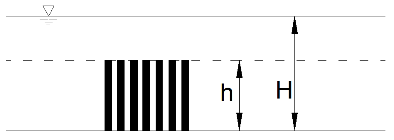
Figure 1. Sketch of the submerged vegetation flow.
Water 15 02638 g001
Figure 2. Comparison between the measured and calculated Manning’s roughness coefficients with Equation (9) (R2 = 0.88) [16,19,20,21,22,23,24,25,26,27].
Water 15 02638 g002
Figure 3. Comparison between the measured and calculated Manning’s roughness coefficients with Yang and Choi’s equation (R2 = −10.83) [16,19,20,21,22,23,24,25,26,27].
Water 15 02638 g003
Figure 4. Comparison between the measured and calculated Manning’s roughness coefficients with Li et al.’s equation (R2 = 0.85) [16,19,20,21,22,23,24,25,26,27].
Water 15 02638 g004
Figure 5. Variation in the Manning coefficient with the vegetation density and floodplain water depth for the emerged vegetation flow.
Water 15 02638 g005
Figure 6. Variation in the Manning coefficient with the vegetation density and floodplain water depth for submerged vegetation flow (vegetation height h = 0.5 m).
Water 15 02638 g006
Figure 7. Variation in the Manning coefficient with vegetation height and floodplain water depth for submerged vegetation flow (vegetation density a = 1 m−1).
Water 15 02638 g007
Figure 8. Schematic of the Duliujian River, revised based on Sun et al. [29].
Water 15 02638 g008
Figure 9. Schematic of the middle reaches of Yangtze River from Chai et al. [30]. The study area is between Chenglingji and Luoshan.
Water 15 02638 g009
Figure 10. Study area image and typical section location.
Water 15 02638 g010
Figure 11. Schematic of the main channel and floodplain zoning of the typical cross section.
Water 15 02638 g011
Table 1. Summary of experiments conducted by previous researchers.
ResearcherVegetation Diameter (mm)Vegetation Height (m)Volume Fraction (%)Vegetation ShapePatternNumber of Runs
Shimizu et al. [19]1–1.50.041–0.0460.44–0.79CylinderLinear28
Dunn et al. [20]6.350.1180.14–1.23CylinderStaggered12
Meijer and van Velzen [21]80.45–1.50.32–1.29CylinderStaggered48
Lopez and Garcia [22]6.40.120.55–1.24CylinderStaggered8
Ghisalberti and Nepf [23]6.40.1381.26–4.02CylinderStaggered11
Murphy et al. [24]6.40.07–0.141.18–3.77CylinderRandom24
Nezu and Sanjou [25]80.05 Flat stripLinear9
Yan [26]60.061.41–5.66CylinderLinear12
Yang [27]20.0350.44CylinderStaggered2
Cheng [16]3.2–8.30.10.41–11.9CylinderStaggered23
Disclaimer/Publisher’s Note: The statements, opinions and data contained in all publications are solely those of the individual author(s) and contributor(s) and not of MDPI and/or the editor(s). MDPI and/or the editor(s) disclaim responsibility for any injury to people or property resulting from any ideas, methods, instructions or products referred to in the content.