Research on the Hydraulic Characteristics of Island Fishways by Experimental and Numerical Methods

Abstract

With the development of hydraulic structures, rivers are becoming fragmented, and their connectivity is greatly affected. Important migratory routes through which fish complete their life processes are hindered. In severe cases, it may lead to the extinction of fish species. As facilities commonly used to assist fish upstreaming, fishways are significant for environmental remediation and have received attention from different scholars. This article proposed a new type of fishway, inspired by Tesla valves with obstructing reverse flow characteristics and classic fishway structures. Due to its characteristic of introducing a water-blocking island structure, it was denominated as an island-style fishway. This work studied an island fishway through a combination of physical models and numerical simulations. The results show that this fishway could achieve various flow patterns suitable for fish migration, and the flow rate control was stable. This study also explored the impact of island spacing arrangement on the turbulent structure of the pool chamber. It was found that when the island distance is set at 1.5d, indicators such as flow velocity and turbulent kinetic energy could achieve significant control effects. However, inappropriate d values might cause adverse effects. This research could provide reference ideas for the design of new fishways.

1. Introduction

The abundance of global dam construction has seriously affected the connectivity of natural rivers and blocked the migration channels of fish. The living environment of fish has been damaged, and in severe cases, it may cause the extinction of fish species [1,2]. The fishway is one of the effective measures to improve river connectivity and protect species diversity [3,4]. Currently, fishways can be mainly divided into classic fishways (i.e., vertical slot, orifice, and overflow weir fishway) and different new-type fishways [5]. These classic fishway designs are usually aimed at a large number of certain fish schools in the river. The classic fishway structure has undergone long-term testing and established its unique advantages. However, natural rivers have different migration periods, and the corresponding migrating fish adapt to different flow rates during each migration period. These fishways may still experience low efficiency in actual operation, so different scholars have also tried to transform and optimize such classic structures [6]. The new style of fishways includes Tai Chi style, C-type, and various combinations of different fishways [7,8,9,10]. Exploring different types of new fishways is one of the popular directions in the current related fields.

This article proposed an island-style fishway, inspired by Tesla valves and classic fishway structures. The Tesla valve is a check valve proposed by Nikolai Tesla in 1920, characterized by its ability to easily allow fluid to flow in one direction while exhibiting strong resistance to reverse flow [11]. Tesla valves without movable components have advantages such as simple structure and long service life, often used in energy and microfluidic control [12,13]. This excellent performance makes Tesla valves possible for application in fishways. In 2016, Delft University of Technology [14] proposed applying large-scale Tesla valves to fishways and conducted relevant experiments. Their experiments have found a “pool-stream-pool” structure in the Tesla valve fishway, which may allow fish to ascend in continuous small steps. The results indicate that the Tesla valve fishway could meet fish migration needs under certain conditions. However, due to experimental limitations, there is a lack of more critical data to determine the potential application of Tesla valves in fishways. Hoek et al. [15] summarized the former’s work and believed that introducing Tesla valves would be beneficial for building FMRs (fish migration rivers). Subsequently, we used numerical simulation to study the application of Tesla valves in fishways [16]. The work studied the internal flow pattern, turbulent kinetic energy, and pressure of Tesla valves as fish-passing pipelines. We compared them with the indicators of different fish-passing objects, verifying the possibility of Tesla valves as fish-passing facilities.

However, the drawbacks of directly applying Tesla valves to fishways are also significant. For example, constructing such fishways may take up too much area (which is unfavorable in limited-area engineering construction). It may be more suitable to design them as open for general fishways. Błotnicki and Gruszczyński [17] proposed to renovate the Tesla valve fishway and design it as a straight-through type consistent with conventional fishways. However, they only made simple structural changes. The flow rate in the Tesla valve circuit was still high, which was not friendly to fish entering the circuit by mistake. The design did not follow the relevant specifications for fishway construction very well and lacked consideration for target fish species and swimming types [18]. Therefore, it is necessary to consider a more comprehensive design for the combination of Tesla valves and fishways, and further research is needed.

The target passing fish selected was grass carp (Ctenopharyngodon idella), a semi-migratory fish and one of the common fish in nature [19,20]. It is naturally mainly distributed in China, Russia, and Bulgaria. Different studies have taken grass carp as the research object [21,22]. In order to continue previous research, grass carp has often been considered as the main analysis object [16].

This study preserved the Tesla valve’s segmented primary loop mechanism (defined as the island) and valve structure. The island fishway proposed in this article aims to maximize the advantages of Tesla valves while combining classic fishways for a more comprehensive design. A preliminary study on the flow characteristics inside an island fishway was conducted through comprehensive hydraulic model experiments and numerical simulation. This work mainly studied the flow characteristics in the pool chamber and the influence of island distance arrangement on the flow characteristics.

2. Materials and Methods

2.1. Experimental Method

The construction and implementation of the experimental platform relied on fluid equipment and an intelligent testing technology laboratory (China Jiliang University). The model was designed according to the fishway design guidelines and basic hydraulic design points, and a physical model was made [23,24]. The model size was determined based on the similarity criterion of gravity. (The Froude criterion is the gravitational similarity criterion. When gravity is the only force driving the flow of two fluids, it represents the proportion of inertia force and gravity, and the gravity effect of the model is similar) [25]. Specific dimensions: The water pool used in the laboratory inspection was 1350 mm long and 200 mm wide (Figure 1), and the depth of the fishway pool was 200 mm. As shown in the figure, the sink was divided into 5 valvular structures (valve-shaped); each chamber had a valvular thickness of 10 mm and a diameter of 40 mm in a semi-circular arc. The spacing between the same-side valvular structures was 400 mm, while the spacing between the different-side valvular structures was 200 mm. The width of the pseudo vertical seam was b = 20 mm. Based on the overall model scale, the basic island shape was determined to be rectangular 2b × b. The distance from the island to the center of the valve circle was defined as d. In the experimental model, d = 1.5b (limited by the experimental model, more exploration of d values is implemented in the numerical simulation section).

The slope of the fishway could be adjusted through supports. The bottom of the physical model was made of stainless steel (with a plate thickness of 15 mm, and water level measurement points were set every 100 mm on the side of the bottom plate to measure the water level with a ruler). The side walls were made of highly transparent organic glass (with a thickness of 15 mm). The origin of the experimental model coordinates was the starting point of the left board; the X-axis was parallel to the bottom and points downstream with the horizontal slot line, the Y-axis was perpendicular to the bottom, and the Z-axis was transverse [26,27]. The valvular and related structures were made of 3D-printed nylon material, and the test island was made of wood. The entire system forms water circulation through the drive pump. The flow control was achieved through ball valves, while the monitoring of emissions was achieved through electromagnetic flow meters (XUNCE, LD-DN25) installed on the circulation pipeline. A dedicated measurement panel had been customized above the pool chamber, which could be used with an open channel flow meter (OUKA, LS300-A) to measure flow velocity at different depths. As shown in Figure 2, the blue solid points were arranged as measurement points, and each plane could achieve a maximum of 78 velocity sampling points (the specific number depends on the model requirements). They were 25 mm apart in the longitudinal direction (X) and 20 mm apart in the transverse direction (Z). The schematic diagram of measurement points for different water layer heights is shown in h1 and h2.

Based on the specific conditions provided by the laboratory, the experiment used a combination of two sets of flow rates and two sets of slopes to test the control group model. Two levels of measurement were selected for each working condition (Q1 = 3.32 m³/h and Q2 = 2.65 m³/h; S1 = 2.27% and S2 = 5.15%; h1 = 12 mm = 0.6b and h2 = 22 mm = 1.1b). Flow control was achieved by driving the pump (SHIMGE, QDX15-7-0.55K3) in conjunction with the valve.

The experimental design used a model without an island as the control model, and experiments were conducted based on a combination of appropriate conditions. The main analysis was the comparison of the flow velocity and water level at the measurement points under the control group to determine the appropriate experimental conditions. Using the previously determined operating conditions, an island was introduced for testing in the model experiment, and the results were compared with the control model results under the same operating conditions.

This setting preliminarily explored the impact of operating conditions on model experiments and selected appropriate operating conditions for comparative experiments and subsequent numerical simulations.

2.2. Numerical Simulation

A computational fluid dynamics model was established based on the previous experiments, and different island spacing arrangements of fishways were explored and evaluated in order to understand hydraulic characteristics of island fishways better and provide potential design assistance.

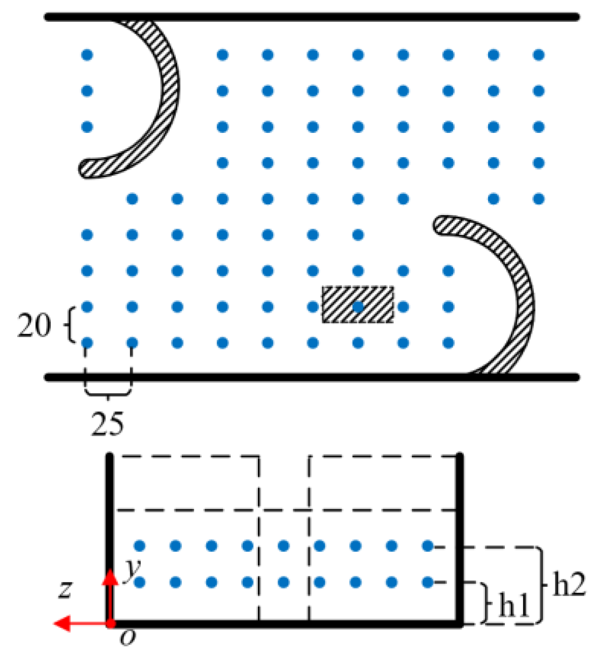
2.2.1. Model Domain and Design Parameters

Figure 3 illustrates the 3D fishway model and structured mesh. Taking the model with experimental islands as an example, the geometric dimensions of the model matched the size of the fishway used in the experiment. The model was validated by measuring the left/right water level lines, mean plane velocity, and corresponding flow structures. Once the model was validated, more exploration of island distance d could be conveniently carried out.

2.2.2. Governing Equations

The numerical simulation of the fishway flow field needs to consider the three major equations of fluid motion, the turbulent characteristics of fluid motion, and the characteristics of the free liquid surface [28,29].

(i)

Turbulence control equation

Numerical experiments used RNG k-ε (based on the renormalization group theory) [30], a mathematical model that can achieve high computational accuracy while saving computational resources in the study of numerical simulation of fish channels. This model mainly includes turbulent kinetic energy k (Equation (1)) and turbulent energy dissipation rate ε (Equation (2)):

$$\begin{array}{c} \frac{\partial \left(\rho k\right)}{\partial t}+\frac{\partial \left(\rho u_{i}k\right)}{\partial x_i}=\frac{\partial }{\partial x_i}\left[\left({\alpha }_k{\mu }_{eff}\right)\frac{\partial k}{\partial x_j}\right]+G_k+G_b-\rho \epsilon -Y_M+S_k\end{array}$$

(1)

$$\begin{array}{c}\frac{\partial \left(\rho \epsilon \right)}{\partial t}+\frac{\partial \left(\rho u_i\epsilon \right)}{\partial x_i}=\frac{\partial }{\partial x_j}\left[{\alpha }_{\epsilon }{\mu }_{eff}\frac{\partial \epsilon }{\partial x_j}\right]+C_{1\epsilon }\frac{\epsilon }{k}\left(G_k+G_{3\epsilon }{G}_b\right)-C_{2\epsilon }\rho \frac{{\epsilon }^2}{k}-R_{\epsilon }+S_{\epsilon }\end{array}$$

(2)

$$\begin{array}{c}{\mu }_{eff}=\mu +{\mu }_t=\mu +C_{\mu }\frac{k^2}{\epsilon }\end{array}$$

(3)

$$\begin{array}{c}{R}_{\epsilon }=\frac{\rho C_{\mu }{\eta }^3\left(1-\frac{\eta }{{\eta }_0}\right){\epsilon }^2}{1+\beta {\eta }^3}\frac{{\epsilon }^3}{k}\end{array}$$

(4)

where $\rho$ is the fluid density; $k$ is turbulent kinetic energy; $u_i$ is velocity tensor; $\epsilon$ is the turbulent dissipation rate; $\mu$ is hydrodynamic viscosity; ${\mu }_{eff}$ is the corrected dynamic viscosity; $x_i$, $x_j$ are coordinate tensors; $G_k$ is the generation phase of turbulent kinetic energy caused by average velocity; $G_b$ is the generation phase of turbulent kinetic energy caused by floating; $Y_M$ is the contribution of pulsation expansion to the overall turbulent dissipation rate in compressible turbulence; $C_{1\epsilon }$, $C_{2\epsilon }, G_{3\epsilon }$ are empirical constants: $C_{1\epsilon }$ = 1.42, $C_{2\epsilon }$ = 1.68, $G_{3\epsilon }$ = 1.72; ${\alpha }_k$ = ${\alpha }_{\epsilon }$= 1.393; $R_{\epsilon }$ is an additional item; $S_k$, $S_{\epsilon }$ is a custom source phase; $\eta$ is the ratio of turbulence time scale to the average time scale: $\eta$ = $S_k$/$\epsilon$; $S$ is the norm of strain rate tensor; $C_{\mu }$ $\beta$ are constants: $C_{\mu }$ = 8.54 × 10⁻², $\beta$ = 0.012; ${\eta }_0$ is the ratio of turbulence time scale to mean flow time scale: ${\eta }_0$ = 4.38.

(ii)

Free surface control equation

Since the fishway of the numerical experiment is an open channel structure, the VOF model, a widely used multiphase flow model, is used to deal with free surface flow. The VOF model can be calculated by solving the momentum equation and following up the whole domain of each fluid volume fraction to the immiscible fluid of two or more models. The model equation is as follows:

$$\begin{array}{c}\frac{\partial {\alpha }_i}{\partial t}+u_j\frac{\partial {\alpha }_i}{\partial x_j}=0\end{array}$$

(5)

In the equation: $u_j$ is the velocity component of each phase; ${\alpha }_i$ is the volume fraction of phase i. This research contains the gas phase (${\alpha }_g$) and aqueous phase (${\alpha }_w$). For the research of the entire model, ${\alpha }_g$ + ${\alpha }_w$ = 0. When ${\alpha }_w$ = 1, it indicates that the water phase fills the entire region; when ${\alpha }_w$ = 0, it indicates that the gas phase fills the entire region.

2.2.3. Mesh and Boundary Conditions

Grid independence studies were conducted on four grid cell sizes M1, M2, M3, and M4, based on a control group (no placement island model, NI) to obtain grid-independent solutions. The numerical simulation was conducted using experimental condition one [31]. The grid-related information and water level comparison results are shown in

Table 1. Experimental model average water level error along measurement points under different grid partitioning schemes.

Mesh Number	Size (m)	Elements	Error (%)
M1	0.01	59,460	7
M2	0.008	112,900	6.08
M3	0.006	257,268	5.95
M4	0.005	461,720	5.98

. The results show that when the M3 scheme is used for the grid, the calculation error caused by the number of grids is already small. Considering computing resources and accuracy, this article’s calculation grid scheme adopted M3 [32]. In addition, a comparison of the average velocity of the 2# pool chamber was conducted in this work, and the average values of a total of 78 measurement points at a relatively stable height of h1 were calculated, which approximated the average velocity of the pool chamber at that height to be 0.178 m/s. The corresponding simulation value was 0.167 m/s, with an error of approximately 6.18%, within the project’s allowable error range [33]. And this verification could reveal a significant error in the high-water layer, indicating that the turbulence near the surface layer in the experiment was intense, and actual measurements were prone to errors. From a numerical perspective, the environment provided by simulation may be ideal, and the results obtained may be more stable than in reality [34].

The numerical calculation platform was based on Fluent 19.1 (ANSYS, Pittsburgh, PA, USA) and in the setting of the numerical calculation method, the model slope was set using the gravity decomposition method. The inlet boundary adopted a pressure inlet, and the flow rate and liquid level values were set depending on the flow rate. The outlet was set as a pressure outlet, and there was no regulation on the outlet water level according to the experimental settings. The top surface was an open boundary, a pressure boundary allowing inflow and outflow. Standard wall parameters were used for each face. The SIMPLE pressure velocity coupling algorithm (the SIMPLE algorithm, called Semi Implicit Method for Pressure Linked Equations, is a widely used numerical method in computational fluid dynamics for solving the flow field) and second-order upwind scheme were adopted [16,31,35]. The number of iteration steps was set to 2000, the maximum iteration step size was 20, and the convergence error was 10⁻⁴. All post-processing and data statistics were conducted in CFD-post.

3. Results and Discussion

3.1. Experimental Results and Model Performance Validation

Regarding the testing of the control group, as shown in Figure 4, under the same working conditions, the changes in the water level along the way were all alternating left and right, with an overall arrangement of left and right steps (1: Q1, S1; 2: Q2, S1; 3: Q1, S2; 4: Q2, S2). The reason for the alternating phenomenon of water level lines was the left and right arrangement of the valve structure in the fishway (due to the arrangement of valves, ideally, the water level lines should have apparent left and right alternating every 200 mm). Meanwhile, the water level measurement results at different measuring points in the control group under different working conditions are shown in Figure 5. Experimental observations found that under the same operating conditions, the water level changed relatively smoothly along the left and right sides of the middle and front parts of the route. In contrast, the difference in water level increased and turbulence became more severe in the rear part due to approaching the outlet. Based on the analysis considerations in this section, the 2# area in the middle and front of the fishway is selected for pool room research in the future. In addition, the comparison under different operating conditions can be found in

Table 2. Average value of water level measurement points under different operating conditions; unit: mm.

No.	${\overline{\mathit{H}}}_{\mathit{m}\mathit{l}}$	${\overline{\mathit{H}}}_{\mathit{m}\mathit{r}}$
1	38.6	40.5
2	31.9	33.6
3	28.1	28.8
4	25.4	26.9
1(I)	40.1	42.2

Note(s): ${\overline{H}}_{ml}$ represents the measured left average water level; ${\overline{H}}_{mr}$ represents the measured right average water level.

, such as comparing operating condition 1 to operating condition 2 (or operating condition 3 to operating condition 4). As the flow rate increased, the overall water level showed a higher performance; however, comparing condition 1 to condition 3 (condition 2 compared to condition 4), it can be seen that an increase in slope would result in a significant change in the water level difference along the way.

Furthermore, as shown in Figure 6, the control group’s flow velocity heat map was obtained under different operating conditions, and water depths were measured. Under all four operating conditions, the highest flow velocity of the h2 water layer near the surface was slightly higher than the flow velocity of the bottom layer h1 in different water layers under the same operating condition. This phenomenon might be caused by the local turbulence of water flow near the surface, which was more severe than that in the bottom layer.

Comparing condition 1 to condition 2 (or condition 3 to condition 4), when the flow rate decreased, the maximum flow rate of the h1 water layer decreased compared to condition 1, while the maximum flow rate of the h2 water layer increased; the average flow velocity was similar for different water layers [36]. Comparing condition 1 to condition 3 (or condition 2 to condition 4), the highest and average flow velocities of different water layers in condition 3 increased with increasing slope compared to condition 1, and the difference in maximum flow velocities of different water layers with higher slope (condition 3) was more significant. Condition 4 presents a relatively chaotic flow pattern under conditions of small flow rate and large slope, which was caused by the fixed height measurement point being too close to the surface under low water level conditions. Based on the above experiments under different operating conditions in the control group, it was determined that the following research would be conducted using operating condition 1, which could be conducive to more stable observation and measurement of water flow patterns.

Overall, the fundamental laws of hydraulic changes in fishways corresponding to different operating conditions can be mastered. The following research focuses on exploring the role of islands in this fishway. Therefore, following the above experiment, a set of island experiments were conducted repeatedly based on the operating conditions, with the island arrangement d = 1.5b in the experiment. Table 2, option 1(I) shows the statistical results related to water level, and the flow field results are shown in Figure 7. In the experimental comparison of adding islands, it was found that the added islands divided part of the mainstream, and the lower part of the mainstream formed a loop. A small area of low flow velocity was formed close to the upper side of the island, which enriched the overall flow pattern. According to the heat map results, it can be seen that after adding the island, the maximum flow velocity measured in the fishway decreased. In contrast, the calculated average flow velocity did not differ much, but the difference in flow velocity between different water layers decreased. In addition, the measured heat map shows that the velocity in the annular region might not be high, indicating that there could still be a low-velocity region near the annular region. The scene would be friendly to fish that stray into the loop. The comparison of the water level after adding the island is shown in Figure 8, where both the left and right water levels increased, resulting in an overall increase in water level. This appearance was also one of the reasons for the narrowing of the difference in water level and velocity between the upper and lower layers. If grass carp were used as a migratory object, according to Yang’s experiment [37], the minimum threshold for stimulating the migration of grass carp could be set to 0.2 m/s, and the flow velocity in the mainstream area measured by the experimental model was greater than this value. The measured maximum flow velocity in the pool chamber was about 0.5 m/s. In combination with other swimming capacity indicators of grass carp of different sizes [38], the flow field, flow velocity, and physiological habits of grass carp in island fishways can be comprehensively considered to realize migration in theory.

3.2. Hydraulic Characteristic Analysis

Overall analysis, combined with experimental comparison, preliminarily determined that the role of the island was positive and practical. Next, the exploration of different turbulence characteristics [39] of the island-style fishway was further carried out through numerical simulation.

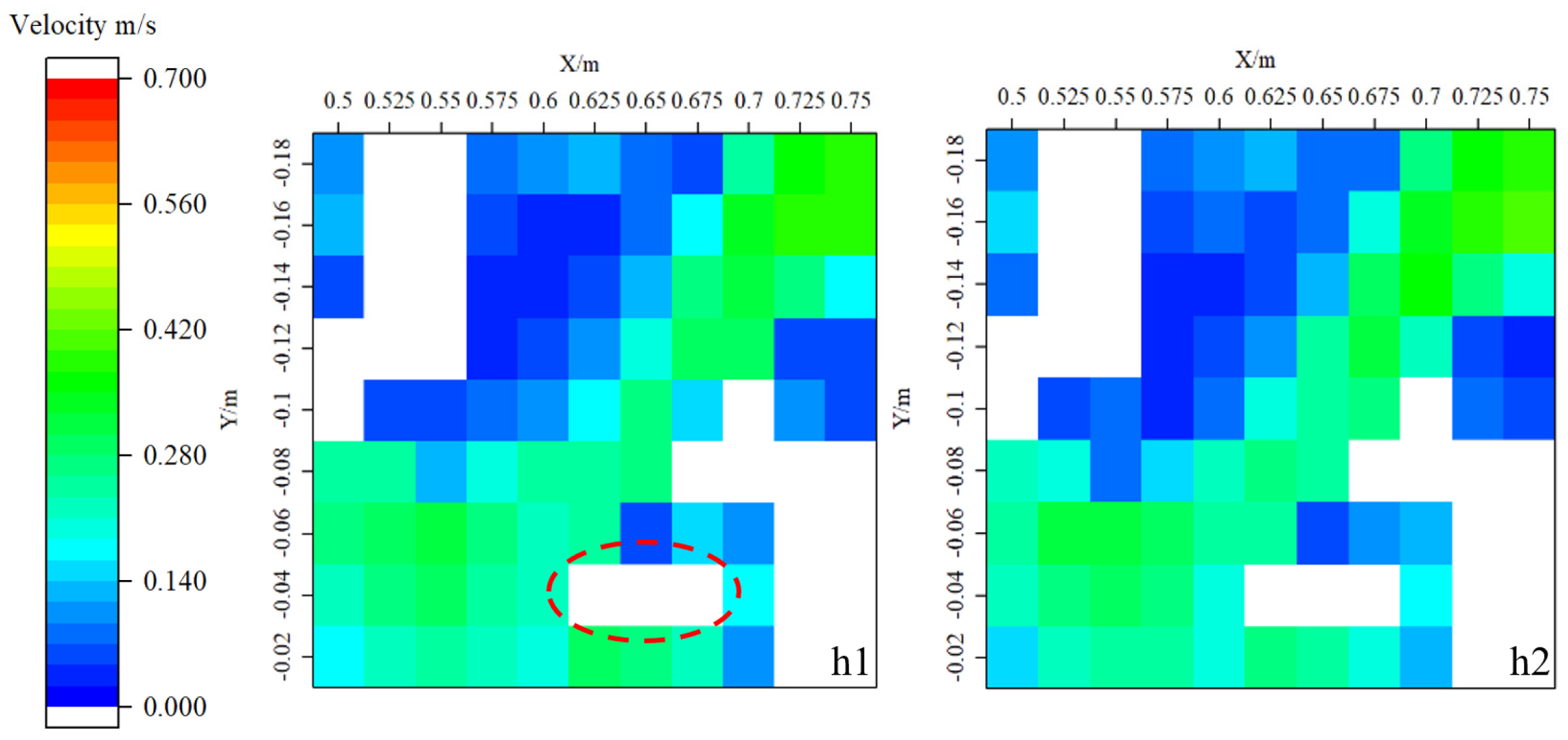
3.2.1. Velocity Field Distribution

The flow velocity is the main hydraulic factor that affects the upward trajectory of fish, and it is also an essential criterion for determining the design of fishways [40]. In this experiment, as shown in Figure 9, there were mainly two flow patterns in different fishway ponds, namely the mainstream region presenting a nearly “S” shape and the reflux region (mainly low flow velocity region) in the upper part of the mainstream region. Studies by different scholars have shown that fish could identify mainstream areas with high flow rates for upstream tracing. In contrast, the reflux area above the mainstream could provide a resting place for their migration process [41,42]. In addition, there was a rich flow pattern around the valve, with the mainstream passing through the pool chamber near the end of the valve. In the island-free (NI) model, there were apparent low flow velocity regions in the front and back regions of the valve. For the pool structure with islands, the high-speed water entering the pool could not directly flow through the pool due to the obstruction of the rectangular island, changing the original flow pattern of the pool. The mainstream area was divided into two by the island, and some of the mainstream was introduced into the loop under the island and lobe structure, forming different flow patterns in the pool chamber.

In order to facilitate a comparative analysis of the impact of island arrangement on the flow field, the distance d values from different islands to the center of the lobe arc were selected. For the convenience of size selection, the pseudo vertical seam width b was used as the dimension, and d values were taken as 0, 1.5b, 3b, 4.5b, and 6b, respectively. And flow field extraction was carried out at heights of h1 and h2. From the results, it can be observed that at the same height, the mainstream was cut by islands, and this segmentation effect increased with the increase in the d value, while the degree of curvature of the mainstream also decreased. The main flow entering the pool chamber was divided into two high-speed streams, each flowing to the left and right sides of the island and converging at the end of the valve. At the same time, the reflux effect at the height of h2 was weaker than that at the height of h1. As the d value increased, the reflux area at the same height generally showed a weakening trend. In addition, due to the flow around the island, a certain low-velocity area was formed behind the island, and this area expanded with the increase in the d value.

Based on the way of dividing the high- and low-velocity regions described in the previous section, the statistical results of the relevant flow rates and areas are shown in

Table 3. Statistics of pool chamber flow field data under different models.

No.	H	${\mathit{U}}_{\mathit{m}\mathit{a}\mathit{x}} (\mathbf{m}/\mathbf{s})$	$\mathit{R}{\mathit{U}}_{\mathit{m}\mathit{a}\mathit{x}} (\%)$	$\overline{\mathit{U}}$	$\mathit{R}\overline{\mathit{U}} (\%)$	${\mathit{U}}_{\mathit{h}}/{\mathit{U}}_{\mathit{l}}$
1	h1	0.538	-	0.167	-	0.575
	h2	0.548	-	0.155	-	0.494
2 (0b)	h1	0.491	−8.740	0.169	1.200	0.524
	h2	0.505	−7.850	0.167	7.740	0.513
3 (1.5b)	h1	0.449	−16.540	0.162	3.000	0.588
	h2	0.456	−16.790	0.156	0.650	0.544
4 (3b)	h1	0.481	−10.590	0.167	0	0.624
	h2	0.453	−17.340	0.166	7.100	0.611
5 (4.5b)	h1	0.486	−9.670	0.182	8.980	0.797
	h2	0.455	−16.970	0.179	15.480	0.713
6 (6b)	h1	0.497	−7.620	0.169	1.200	0.587
	h2	0.496	−9.490	0.173	11.610	0.612

. The results show that after adding the island, compared to the control group without the island, the maximum flow velocity decreased. From the maximum flow velocity change rate, it can be seen that when d = 1.5b, the inhibition effect on the maximum flow velocity of different water layers was the best. The experimental results in the same section are consistent. The severe local turbulence results in a slightly higher maximum velocity of surface hydrogen than in the h1 layer, but overall, the velocity of the two layers is similar [43]. From the change rate of average velocity in the pool chamber, it can be seen that the average velocity after adding islands had increased compared to the model without islands. When d = 1.5b, the variation of average velocity was slight, considering the performance of average velocity in different water layers.

As shown in Figure 10, with the addition of islands, the maximum flow velocity in the pond chamber shows a trend of first decreasing and then increasing as the d value increases. The maximum flow velocity of different models meets the migration conditions of grass carp, and good results can be achieved near d = 1.5b; as shown in Figure 11, the overall average flow velocity in the pool chamber shows an upward trend with the increase in island distance. When d = 3b and 4.5b, the velocity of the h2 layer begins to be lower than that of the h1 layer. This phenomenon indicates that under the action of the island, the maximum velocity of the upper water level can be further reduced. From the corresponding velocity change rates in Figure 10a,b, it can be seen that the deceleration effect of these two models at the h2 height was relatively significant. From this perspective, the island might have an impact on the three-dimensional characteristics of the fishway. After adding the island, the average water layer difference between the upper and lower layers of the model decreased, with the maximum difference decreasing from 0.012 to 0.006 m/s. The water flow was relatively more stable, and the reflux was relatively weakened. However, overall, in the third model (d = 1.5b), the deceleration effect of both water layers was very significant.

The area ratio U_h/U_l of the high and low flow velocity regions is shown in Table 3. After joining the island, when d was set to 0, it had a certain inhibitory effect on the high flow velocity area of the h1 layer. After d further increased, the high flow velocity area showed an increasing trend; especially when d = 4.5b, the low flow velocity area dropped to the lowest. This situation might lead to fish not being able to have sufficient rest during migration, reducing fish passing efficiency. However, the h2 layer did not show a significant inhibitory effect on high-velocity regions. The visual expression of the relevant results is shown in Figure 12.

3.2.2. Turbulent Kinetic Energy

Turbulent kinetic energy (TKE) reflects the amplitude of flow velocity fluctuations and is one of the critical parameters affecting fish passage. Fish need to consume more energy to resist turbulence in high-TKE turbulence [44]. At the same time, highly turbulent water flow may also prolong the time for fish to successfully pass through the fishway, affecting the efficiency of fish passage. As shown in Figure 13, the TKE at h2 height was significantly higher than that at h1 height in all models, which was caused by more intense turbulence near the water surface. In the island-free (NI) model, the high turbulence region in the pool mainly existed before and after the valve structure, and then extended to the wall area of the mainstream impact. Compared to conventional pool chambers, the distribution of TKE began to change after adding islands to the pool chamber. At d = 0, the TKE significantly decreased compared to the NI model, with higher levels of TKE present in the small area at the front of the valve and the impact of the mainstream and the chamber wall; when d = 1.5b, the average TKE of the pool chamber was minimized. However, as the d value continues to increase, TKE continues to increase, and TKE begins to undergo significant changes. As shown in

Table 4. TKE data statistics for different models.

No.	H	$\mathit{T}\mathit{K}{\mathit{E}}_{\mathit{m}\mathit{a}\mathit{x}} (\times {10}^{-3} {\mathbf{m}}^2/{\mathbf{s}}^2)$	$\mathit{R}\mathit{T}\mathit{K}{\mathit{E}}_{\mathit{m}\mathit{a}\mathit{x}} (\%)$	$\overline{\mathit{T}\mathit{K}\mathit{E}} (\times {10}^{-3} {\mathbf{m}}^2/{\mathbf{s}}^2)$	$\mathit{R}\overline{\mathit{T}\mathit{K}\mathit{E}} (\%)$
1	h1	4.62	-	1.62	-
	h2	5.54	-	1.99	-
2 (0b)	h1	3.70	−19.91	1.29	−20.37
	h2	4.73	−14.62	1.74	−12.56
3 (1.5b)	h1	3.98	−13.85	1.15	−29.01
	h2	4.83	−12.82	1.51	−24.12
4 (3b)	h1	4.53	−1.95	1.42	−12.35
	h2	6.34	14.44	1.91	−4.02
5 (4.5b)	h1	5.42	17.32	2.10	29.63
	h2	6.49	17.15	2.81	41.21
6 (6b)	h1	6.34	37.23	2.07	27.78
	h2	7.77	40.25	2.79	40.20

Note(s): H: water layer height; $TK{E}_{max}$: maximum turbulent kinetic energy of the pool chamber; $RTK{E}_{max}$: at the same water layer height, the change rate of maximum turbulent kinetic energy in the pool chamber compared to the control group; $\overline{TKE}$: average turbulent kinetic energy of the pool chamber; $R\overline{TKE}$: at the same water layer height, the change rate of average turbulent kinetic energy in the pool chamber compared to the control group.

, the average TKE value of the pool chamber reaches its maximum at d = 4.5b; when d = 6b, the maximum value of TKE appears at the end of the valve structure, which is due to the most significant effect of island segmentation on the mainstream. Two high-speed water streams met at the valve end, causing high turbulence in the water flow. Scholars recommend that the turbulent kinetic energy of the pool chamber should be kept below 0.05 m²/s² [45], but due to the low slope of the experiment, the turbulence intensity was not high [41]. Different pool structures’ maximum TKE did not exceed the range.

Figure 14 and Figure 15 show that the island distance d had a consistent improvement pattern for TKE in different water layers. For the maximum TKE, as the d value increased to 3b, the TKE began to weaken and become stronger; The weakening effect of the average TKE was most significant when d = 1.5b, and further increasing the value of d also increased the average TKE. After d reached 4.5b, the variation pattern stabilized. The corresponding change might be due to the varying degrees of deviation from the model’s mainstream center where the island was located.

3.2.3. Water Depth Distribution

As shown in Figure 16, the changes in water depth along the left, right, and centerline are shown from top to bottom (the last lobe is set at a height of 1.1 m, and the disturbance of the water level near the outlet could not be considered). From the left and right sides, it can be observed that the water level ladder alternates left and right, which is consistent with the experimental results. The arrangement of the left and right lobe structures influenced alternating the left and right water levels. The valve structure was located at 0.3 m, 0.7 m, and 1.1 m on the left side, while the corresponding structure on the right was located at 0.5 m and 0.9 m, consistent with the design intent. In order to better observe the changes in water level, the water level along the centerline was also obtained here. The figure shows that the effect was consistent with the structural design, with step changes occurring at the centerline position every 0.2 m. The midline, as the central upstream passage for fish, had a much smoother change in water level compared to the left and right sides.

The variation pattern of water level along the way is consistent with the control models of different experiments. However, the difference lies in adding islands to the model, which resulted in a certain increase in water level. From the changes in water level on the left and right sides, it can be observed that the fluctuation of water level was relatively large at d = 3b, 4.5b, and 6b. From the locally enlarged view along the centerline, it can be observed that the effect of water level increase was most significant when d = 0 and 1.5b. Although the changes in water depth were not as significant as the changes in flow velocity and TKE discussed earlier, achieving an appropriate distance from the island could still benefit water level rise.

From

Table 5. Statistical data of pool chamber water level; unit: mm.

No.	Hsl (mm)	RHsl (%)	Hsr (mm)	RHsr (%)	Hsm (mm)	RHsm (%)
1	44.84	-	41.14	-	38.34	-
2	45.46	1.38	42.41	3.09	39.72	3.60
3	45.04	0.45	42.96	4.42	39.95	4.20
4	44.44	−0.89	42.33	2.89	38.86	1.36
5	42.92	−4.28	40.81	−0.80	36.52	−4.75
6	42.59	−5.02	40.66	−1.17	37.51	−2.16

Note(s): H_sl: left average water level statistics; H_sr: right average water level statistics; H_sm: middle average water level statistics; taking RH_s1 as an example, it represents the water level change rate of the control group.

of the statistical data, it can be seen that the island distance with the effect of raising the water level should be taken as 0 or 1.5b; from Figure 17, it can be observed that when 3b was taken, and the value of d continued to increase, the water level did not rise but began to decrease. The trend of water level changes in the left, middle, and right directions was consistent, while the trend of water level changes in the central line was basically between the changes on the left and right sides. In addition, in Figure 17b, it can be observed that in the case of consistent changes in water levels on different sides, this change produced a deviation phenomenon; that is, at the initial d value (i.e., 0, 1.5b), the water level change rate on the right side was higher than that on the left side. The possible reason is that the right side referred to here is the upper side of the main flow, and under different models, most of the main flow passes through the upper side of the impact pool wall, which easily forms water level accumulation. At this point, the remaining part of the segmented mainstream enters one side of the island circuit, which has the effect of water accumulation. However, the flow rate of this part is significantly lower than that of the other side, which also causes different effects of water flow changes. However, as the d value increased, the distribution of mainstream segmentation also began to change, with an increase in the flow entering the circuit and a more significant decrease in the water level on the left. The reason was that as the value of d increased, the distance between the island and the valve gradually increased. The accumulation effect of the water flow on this side needed to be achieved through the joint action of the island and the valve. Excessive d led to the gradual weakening of the valve structure, making it more difficult for the fluid entering the circuit to achieve the accumulation effect.

4. Conclusions

This work proposed a new type of island fishway that combines inspiration from Tesla valves with hydraulic design. The flow characteristics of the pool chamber under different island spacing arrangements of the fishway were studied using experimental and simulation methods. From the analysis of different indicators, it is found that island fishways have the primary conditions for fish migration. The research conclusions are as follows:

(1)

The main flow area of the fishway was evident in the pool chamber. Additionally, the rear of the island structure presented a small area of low flow velocity, and this area tended to elongate with the increase in island distance setting. The proportion of high and low flow velocity areas varied little under different pool layout schemes, while low flow velocity areas often accounted for over 60% of the pool area.

(2)

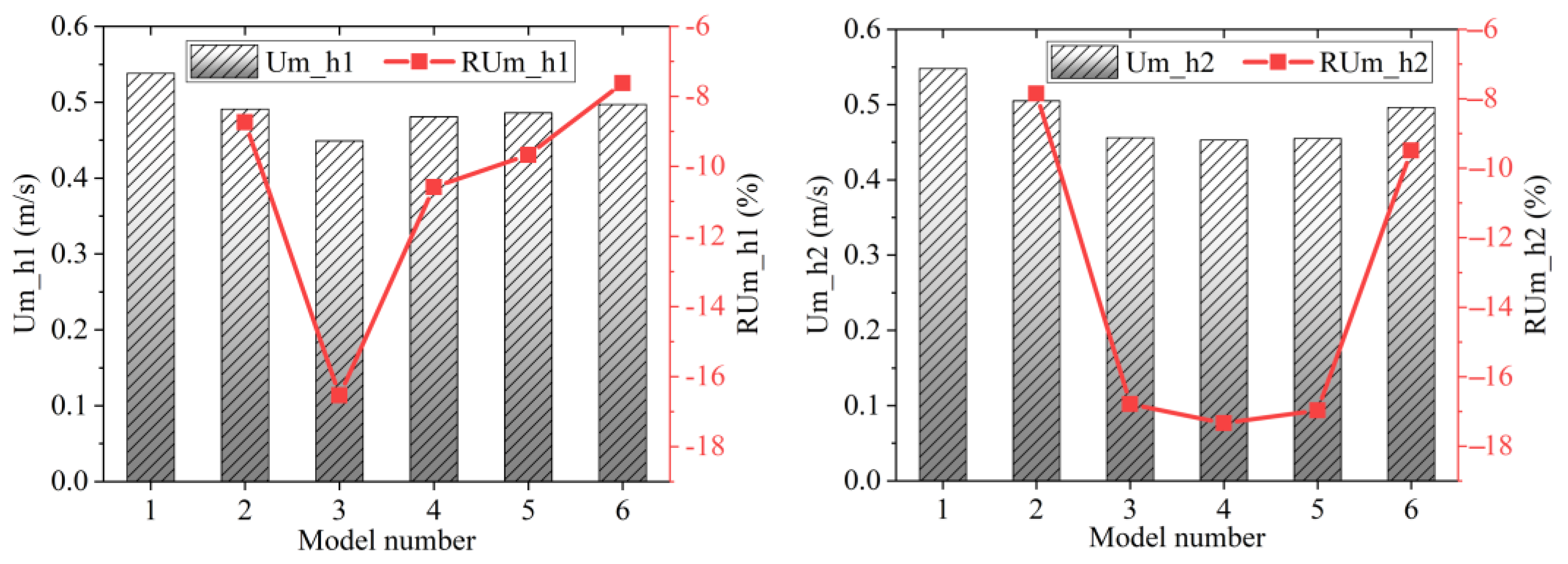
The upper layer’s maximum flow velocity was higher than that of the lower layer, while the average velocity was similar. The arrangement of the island significantly suppresses the maximum flow velocity of different water layers (d = 1.5b having a better effect). However, this inhibitory effect weakens as the island distance increases; for the average flow velocity, the effect of the island leads to a slight increase, and as the island distance increases, the overall effect tends to intensify.

(3)

The distribution of TKE values in the upper layer was significantly higher than that in the lower layer. When d was taken as 0 or 1.5b, it had an excellent inhibitory effect on TKE, with a maximum weakening TKE value of up to 30%. Overall, TKE values showed an increasing trend with increasing d values, with a maximum increase of approximately 40% (d = 6b; h2). The average turbulent kinetic energy in the pool chamber was relatively small, and the maximum turbulent kinetic energy in the pool chamber was less than 0.01s²/m².

(4)

The water level showed a stepped distribution as a whole. The results show that its changes were not significant under different models, and there was only a certain effect of raising the water level when d = 0 and 1.5b. However, further increasing the d value might even lead to a slight decrease in the water level. Combined with the above flow rate and TKE analysis, it could be considered appropriate to take a value near 1.5b for d.

References

1. Katopodis, C.; Cai, L.; Johnson, D. Sturgeon survival: The role of swimming performance and fish passage research. Fish. Res. 2019, 212, 162–171. [Google Scholar] [CrossRef]
2. Huang, Z.; Wang, L. Yangtze dams increasingly threaten the survival of the Chinese sturgeon. Curr. Biol. 2018, 28, 3640–3647.e3618. [Google Scholar] [CrossRef]
3. Mallen-Cooper, M.; Brand, D. Non-salmonids in a salmonid fishway: What do 50 years of data tell us about past and future fish passage. Fish. Manag. Ecol. 2007, 14, 319–332. [Google Scholar] [CrossRef]
4. Williams, J.G.; Armstrong, G.; Katopodis, C.; Larinier, M.; Travade, F. Thinking like a fish: A key ingredient for development of effective fish passage facilities at river obstructions. River Res. Appl. 2012, 28, 407–417. [Google Scholar] [CrossRef] [Green Version]
5. Mao, X. Review of fishway research in China. Ecol. Eng. 2018, 115, 91–95. [Google Scholar] [CrossRef]
6. Kasischke, K.; Oertel, M. Discharge Coefficients of a Specific Vertical Slot Fishway Geometry—New Fitting Parameters. Water 2023, 15, 1193. [Google Scholar] [CrossRef]
7. Qie, Z.; Guo, L.; Wu, X.; Ran, Y. Experimental study and numerical simulation of hydraulic characteristics of Tai Chi fishway. Trans. Chin. Soc. Agric. Eng. 2018, 34, 182–188. [Google Scholar]
8. Baharvand, S.; Lashkar-Ara, B. Hydraulic design criteria of the modified meander C-type fishway using the combined experimental and CFD models. Ecol. Eng. 2021, 164, 106207. [Google Scholar] [CrossRef]
9. Masumoto, T.; Nakai, M.; Asaeda, T.; Rahman, M. Effectiveness of New Rock-Ramp Fishway at Miyanaka Intake Dam Compared with Existing Large and Small Stair-Type Fishways. Water 2022, 14, 1991. [Google Scholar] [CrossRef]
10. Dong, Z.; Tong, J.; Huang, Z. Turbulence characteristics in a weir-orifice-slot combined fishway with an identical layout. J. Turbul. 2022, 23, 327–351. [Google Scholar] [CrossRef]
11. Thompson, S.M.; Paudel, B.; Jamal, T.; Walters, D. Numerical investigation of multistaged tesla valves. J. Fluids Eng. 2014, 136, 081102. [Google Scholar] [CrossRef]
12. Qian, J.-Y.; Wu, J.-Y.; Gao, Z.-X.; Wu, A.; Jin, Z.-J. Hydrogen decompression analysis by multi-stage Tesla valves for hydrogen fuel cell. Int. J. Hydrogen Energy 2019, 44, 13666–13674. [Google Scholar] [CrossRef]
13. Zhang, S.; Winoto, S.; Low, H. Performance simulations of Tesla microfluidic valves. In Proceedings of the International Conference on Integration and Commercialization of Micro and Nanosystems, Sanya, China, 10–13 January 2007; pp. 15–19. [Google Scholar]
14. Keizer, K. Determination Whether a Large Scale Tesla Valve Could Be Applicable as a Fish Passage. Additional Thesis, Delft University of Technology, Delft, The Netherlands, 2016. [Google Scholar]
15. Hoek, S.; Jin, R.; van der Schaar, E.; Shanitbayeva, S.; de Visser, M.; Wallace, N.; Lavooij, H. The Return of Fish Migration to the Dutch River Delta. 2021. Available online: https://www.delta21.nl/wp-content/uploads/2022/02/ACT-Vismigratierivier.pdf (accessed on 13 July 2023).
16. Zeng, G.; Xu, M.; Mou, J.; Hua, C.; Fan, C. Application of Tesla Valve’s Obstruction Characteristics to Reverse Fluid in Fish Migration. Water 2022, 15, 40. [Google Scholar] [CrossRef]
17. Błotnicki, J.; Gruszczyński, M. Modelling of Tesla Valvular Concuit as an Energy Dissipation System in Fish Pass Pools. In Proceedings of the 2nd International Scientific Conference on Ecological and Environmental Engineering COEE21, Wrocław, Poland, 30 June–1 July 2021; p. 6. [Google Scholar]
18. Webb, P.W.; Kostecki, P.T.; Don Stevens, E. The Effect of Size and Swimming Speed on Locomotor Kinematics of Rainbow Trout. J. Exp. Biol. 1984, 109, 77–95. [Google Scholar] [CrossRef]
19. Sullivan, C.J.; Weber, M.J.; Pierce, C.L.; Camacho, C.A. A Comparison of Grass Carp Population Characteristics Upstream and Downstream of Lock and Dam 19 of the Upper Mississippi River. J. Fish Wildl. Manag. 2020, 11, 99–111. [Google Scholar] [CrossRef] [Green Version]
20. Masser, M.P. Using Grass Carp in Aquaculture and Private Impoundments; SRAC: Mississippi, MS, USA, 2002. [Google Scholar]
21. Mu, X.; Zhen, W.; Li, X.; Cao, P.; Gong, L.; Xu, F. A Study of the Impact of Different Flow Velocities and Light Colors at the Entrance of a Fish Collection System on the Upstream Swimming Behavior of Juvenile Grass Carp. Water 2019, 11, 322. [Google Scholar] [CrossRef] [Green Version]
22. Xu, M.; Ji, B.; Zou, J.; Long, X. Experimental investigation on the transport of different fish species in a jet fish pump. Aquac. Eng. 2017, 79, 42–48. [Google Scholar] [CrossRef]
23. General Institute of Water Resources and Hydropower Planning and Design. Guidelines for Fishway Design of Water Conservancy and Hydropower Projects; SL 609-2013; China Water & Power Press: Beijing, China, 2013. [Google Scholar]
24. Keming, A. Basic Points and Engineering Examples of Hydraulic Design for Fishways. Water Conserv. Sci. Technol. Econ. 2012, 18, 82–85. [Google Scholar]
25. Yagci, O. Hydraulic aspects of pool-weir fishways as ecologically friendly water structure. Ecol. Eng. 2010, 36, 36–46. [Google Scholar] [CrossRef]
26. Tan, J.; Liu, Z.; Wang, Y.; Wang, Y.; Ke, S.; Shi, X. Analysis of Movements and Behavior of Bighead Carps (Hypophthalmichthys nobilis) Considering Fish Passage Energetics in an Experimental Vertical Slot Fishway. Animals 2022, 12, 1725. [Google Scholar] [CrossRef] [PubMed]
27. Shi, K.; Li, G.; Liu, S.; Sun, S. Experimental study on the passage behavior of juvenile Schizothorax prenanti by configuring local colors in the vertical slot fishways. Sci. Total Environ. 2022, 843, 156989. [Google Scholar] [CrossRef]
28. Cea, L.; Pena, L.; Puertas, J.; Vázquez-Cendón, M.; Peña, E. Application of several depth-averaged turbulence models to simulate flow in vertical slot fishways. J. Hydraul. Eng. 2007, 133, 160–172. [Google Scholar] [CrossRef]
29. Tan, J.; Gao, Z.; Dai, H.; Yang, Z.; Shi, X. Effects of turbulence and velocity on the movement behaviour of bighead carp (Hypophthalmichthys nobilis) in an experimental vertical slot fishway. Ecol. Eng. 2019, 127, 363–374. [Google Scholar] [CrossRef]
30. Barton, A.F.; Keller, R.J. 3D free surface model for a vertical slot fishway. In Proceedings of the XXX IAHR Congress, AUTh, Thessaloniki, Greece, 24 August 2003; pp. 409–416. [Google Scholar]
31. Zhong, Z.; Ruan, T.; Hu, Y.; Liu, J.; Liu, B.; Xu, W. Experimental and numerical assessment of hydraulic characteristic of a new semi-frustum weir in the pool-weir fishway. Ecol. Eng. 2021, 170, 106362. [Google Scholar] [CrossRef]
32. Xu, M.; Zeng, G.; Wu, D.; Mou, J.; Zhao, J.; Zheng, S.; Huang, B.; Ren, Y. Structural Optimization of Jet Fish Pump Design Based on a Multi-Objective Genetic Algorithm. Energies 2022, 15, 4104. [Google Scholar] [CrossRef]
33. Moriasi, D.N.; Arnold, J.G.; Van Liew, M.W.; Bingner, R.L.; Harmel, R.D.; Veith, T.L. Model evaluation guidelines for systematic quantification of accuracy in watershed simulations. Trans. ASABE 2007, 50, 885–900. [Google Scholar] [CrossRef]
34. Jiang, Y.; Alexander, D.; Jenkins, H.; Arthur, R.; Chen, Q. Natural ventilation in buildings: Measurement in a wind tunnel and numerical simulation with large-eddy simulation. J. Wind. Eng. Ind. Aerodyn. 2003, 91, 331–353. [Google Scholar] [CrossRef]
35. Qie, Z.; Liu, H.; Wu, M.; Ran, Y. Establishment of swirling-flow fishway and analysis of its hydraulic characteristics. Trans. Chin. Soc. Agric. Eng. 2020, 36, 126–131. [Google Scholar]
36. Li, H.; Wang, X.; Zheng, F. Analysis of three-dimensional characteristics of water flow in trapezoidal fishways. J. Hohai Univ. (Nat. Sci.) 2022, 51, 1–7. [Google Scholar]
37. Yang, Q.; Hu, P.; Yang, Z.; Chu, L.; Yang, J. Suitable Flow Rate and Adaptive Threshold for Grass Carp (Ctenopharyngodon idellus) Migration. J. Hydroecol. 2019, 40, 93–100. [Google Scholar]
38. Lu, B.; Liu, W.; Liang, Y.; Chen, Q.; Huang, Y.; Pan, L.; Liu, D.; Shi, X. The burst-coast swimming behavior of grass carp (Ctenopharyngodon idellus) during fast-start. J. Fish. China 2014, 38, 6. [Google Scholar]
39. O’Connor, J.; Hale, R.; Mallen-Cooper, M.; Cooke, S.J.; Stuart, I. Developing performance standards in fish passage: Integrating ecology, engineering and socio-economics. Ecol. Eng. 2022, 182, 106732. [Google Scholar] [CrossRef]
40. Hou, Y.; Yang, Z.; An, R.; Cai, L.; Chen, X.; Zhao, X.; Zou, X. Water flow and substrate preferences of Schizothorax wangchiachii (Fang, 1936). Ecol. Eng. 2019, 138, 1–7. [Google Scholar] [CrossRef]
41. Chen, B.; Yuan, H.; He, X.; Sun, Q.; Xu, G. Research on the Influence of Tank Chamber Structure on the Hydraulic Characteristics of Vertical Fishway. J. Yangtze River Sci. Res. Inst. 2022, 1–8. [Google Scholar]
42. Gao, L.; Gao, B.; Xu, D.; Peng, W.; Lu, J. Multiple assessments of trace metals in sediments and their response to the water level fluctuation in the Three Gorges Reservoir, China. Sci. Total Environ. 2019, 648, 197–205. [Google Scholar] [CrossRef] [PubMed]
43. Wu, S.; Rajaratnam, N.; Katopodis, C. Structure of flow in vertical slot fishway. J. Hydraul. Eng. 1999, 125, 351–360. [Google Scholar] [CrossRef]
44. Enders, E.C.; Boisclair, D.; Roy, A.G. The effect of turbulence on the cost of swimming for juvenile Atlantic salmon (Salmo salar). Can. J. Fish. Aquat. Sci. 2003, 60, 1149–1160. [Google Scholar] [CrossRef]
45. Quaranta, E.; Katopodis, C.; Revelli, R.; Comoglio, C. Turbulent flow field comparison and related suitability for fish passage of a standard and a simplified low-gradient vertical slot fishway. River Res. Appl. 2017, 33, 1295–1305. [Google Scholar] [CrossRef]
Figure 1. Experimental system diagram: plan schematic diagram of island fishway and pool chamber structure.
Water 15 02592 g001
Figure 2. Arrangement diagram of flow velocity measurement points in the pool chamber.
Water 15 02592 g002
Figure 3. Grid division diagram of island fishway experimental model.
Water 15 02592 g003
Figure 4. Stepped flow patterns exhibited in experimental testing of island fishway models.
Water 15 02592 g004
Figure 5. Water level map of measuring points along the experimental model (data example: Wline1_1 represents the left water level line under condition 1; Wline1_2 represents the right under condition 1; the red range represents the research pool section).
Water 15 02592 g005
Figure 6. Thermal diagram of measuring point flow velocity.
Water 15 02592 g006
Figure 7. Thermal diagram of flow velocity at measuring points in island fishway (Mark Island).
Water 15 02592 g007
Figure 8. Comparison of the results of water level measurement points on the left (a) and right (b) sides of the island and island-free experimental models.
Water 15 02592 g008
Figure 9. Cloud maps of the flow field in the fishway pool chamber under different models.
Water 15 02592 g009
Figure 10. Maximum velocity and rate of change compared to the control group (Um: maximum velocity; RUm: maximum velocity change rate compared to the control model), including the situation of two water layers, h1 and h2.
Water 15 02592 g010
Figure 11. Average velocity and rate of change compared to the control group (Ua: average velocity; RUa: average velocity change rate compared to the control model), including the situation of two water layers, h1 and h2.
Water 15 02592 g011
Figure 12. The proportion of high- and low-velocity areas in different models.
Water 15 02592 g012
Figure 13. Cloud maps of pool chamber TKE changes for different models.
Water 15 02592 g013
Figure 14. Maximum TKE and rate of change compared to the control group.
Water 15 02592 g014
Figure 15. Average TKE and rate of change compared to the control group.
Water 15 02592 g015
Figure 16. Changes in water flow along the route (the sequence is left, right, middle, and local amplification).
Water 15 02592 g016
Figure 17. The water levels of different lines and the rate of change compared to the control model: (a) the average water level under different paths along the route; (b) the average water level error under different paths relative to the control model.
Water 15 02592 g017