Verification of Hydraulic Parameters of Nature-like Fish Pass

Abstract

Nature-like fish passes are commonly designed as a preferred way to overcome barriers in rivers. However, meeting the recommended hydraulic parameters for these passes can be challenging. As a result, boulders or sills are often incorporated to supplement their structure. From a hydraulic standpoint, the crucial parameters under investigation are the depths and velocities (or the corresponding velocity field). In this study, a comprehensive analysis was conducted on a full-width rock-ramp fish pass constructed in a river, specifically targeting the barbel zone. The achieved parameters were assessed through direct field measurements, complemented by mathematical modeling using 1D and 2D HEC-RAS models (version 6.3.1). For the assessment of model accuracy, the error indices root mean square error (RMSE) and mean absolute error (MAE) were used. Based on their evaluation, the 1D model provides more precise results in the assessed profiles (the RMSE for depths (m) was 0.0663 (for velocities (m∙s⁻¹) 0.293) compared to the 2D model, where the RMSE for depths (m) was 0.070 (for velocities (m∙s⁻¹) 0.398), the MAE for the 1D model for depths (m) was 0.0350 (for velocities (m∙s⁻¹) 0.185) compared to the 2D model, where the MAE for depths (m) was 0.0375 (for velocities (m∙s⁻¹) 0.274)). The findings highlight the differences in the problem-solving approaches between the models as well as the potential for simplifications in practical applications.

1. Introduction

A fish facility, known in general as a fishway, fish ladder, or fish pass, is essentially a water passage around or through an obstruction, designed to dissipate the energy in the water in such a manner as to enable fish to ascend without undue stress [1]. In the context of the Water Framework Directive, the continuity of rivers must be restored by removing barriers. Because it is not possible to remove all barrier structures (e.g., dams, weirs, culverts, sills, etc.), fish passes can help to improve the passability of these barriers and restore the interrupted continuity of streams. [2]. In general, fish passes can be divided into two main groups—technical and nature-like, respectively. The technical fish passes have been examined in the past in detail by many authors [1,3,4,5,6], and detailed methodologies for their design have been created in some countries [7,8]. To achieve the required design parameters for the technical fish passes (pool [9,10], vertical slot [11], or brush-furnished passes [12]) is less demanding than for nature-like ones.

Nowadays, close to natural structures are preferred in many areas of hydraulic design. Nature-like fish passes are often the solution for ecologically oriented river engineering, considering ecology and stream hydraulics [13,14,15]. A nature-like fish pass is a construction that is designed to imitate the environment of the stream and thus provide a natural condition for the ichthyofauna to swim upstream and downstream, respectively. In such a fish pass, the flow is directed through natural-looking elements such as boulders and rocks that help reduce velocities and increase water depths. These components are designed to create flow shadows and pools that provide resting and refuge areas for fish during their migration through the fish pass. The classification of these structures depends on the boulder arrangement inside the fish pass (rock ramp, pool–weir-type, etc.).

Rock-ramp fish passes were developed as a simple and relatively low-cost design compared to more-formally engineered fish passes, particularly for overcoming low barriers and river bed erosion-control structures [16]. These can be conducted as full or partial-width rock-ramp fish passes (e.g., Rock-Ramp Fishway, Cape Fear River Dam, USA). Both types of fish passes are particularly suited for providing fish passage on low weirs, drop structures (approximately up to a height of 2 m) [17], or fixed sills for diversion small hydropower plants. This type of fish pass is characterized by a fast but continuous barrier-free flow that imitates the stream or river. It is shallower, longer, and has a less voluminous water environment compared to other types of fish passes, so it needs a higher flow supply, which depends on the stream hydrology. The fishes in it have to expend an increased amount of energy to overcome the barrier, which many of them cannot do on long routes without creating resting flow shadows, which are formed due to solitary boulders protruding above the river bed bottom [17]. The advantage of these constructions is their aesthetic integration within the landscape. In addition, they have lower implementation and maintenance costs compared to other possible solutions [16], but the cost effectiveness of rock-ramp fish passes differs on many factors, e.g., the block placement, block size, slope, etc. [18]. The positive aspect of the design is the smooth flow of water and the location. On the other hand, the disadvantages include the risk of insufficient flow in dry hydrologic periods and, conversely, the instability of the structure during floods [19]. Flow in ramps is characterized by the continuous damping of flow energy associated with turbulence and aeration because of boulders implemented in the body of the structure. Ramps require a direct route, and a change in direction is only possible in resting pools that are inserted between sections that the fish can overcome in one run. For the bed of the fish pass, a higher roughness is required, usually created by a grid of stones with a medium grain size of at least 0.25 m [20].

Due to the complex structure and the multiformity of the boulder arrangements, there is currently no perfect design criterion for nature-like fishways [21]. To assess the roughness of the used bed material is another complex problem in the design of these structures. The Manning’s roughness coefficient, representing the energy loss, is one of the most important parameters in hydraulic calculations in open channels. Roughness has an important effect on the accuracy of the flow simulations, but its correct determination is rather difficult. In general, the determination of the bed’s roughness is very subjective in practice [22]. The value of the Manning’s roughness coefficient increases with increasing turbulence and higher resistance of the bed against the flow. In sections of water courses, where there is a uniform slope, and where the roughness of the bed and banks is approximately the same, a constant value of the Manning coefficient can be used. In natural river beds, roughness varies with the water depth. The value of the coefficient decreases according to submerging of different elements in the bed (stones, wood, etc.) below the water level. The coefficient, therefore, has a different value at the same location according to the actual water level. For lower flow rates, its value is higher than for higher flow rates. This trend can be reversed in river beds that have a smooth bed, but the banks are densely overgrown with vegetation [23,24].

This paper focuses on the comparison of the parameters of full-width rock-ramp, nature-like fish passes built in barbel fish zones using in-field measurements and 1D and 2D mathematical models. The investigated variables are the Manning’s roughness coefficients, velocities, depths, and widths in the water levels. A verification of the parameters resulting from mathematical modeling can provide recommendations to improve the variable limits given for the fish-pass design.

2. Materials and Methods

In general, rock ramps as a fish-pass structure have prescribed slope of 1:20 or less (1:20 to 1:30) [7,16] or unstructured block ramps as fish-friendly structures have a prescribed slope of 1–3% [25], which is not easy to achieve when designing the structure to not exceed the maximum flow velocity of v_max = 1.6–2.0 m∙s⁻¹. To deal with this problem, boulder elements are embedded into the bed of the ramp. Prescribed parameters depend on national methodologies and zonation of the streams. In the Slovak Republic, according to the valid decree no. 383/2018 [26] (on technical conditions of fish-pass design and monitoring of migration passability of fish passes), limits for full-width rock-ramp, nature-like fish passes are much stricter.

2.1. Parameters and Assessment of Investigated Fish Pass

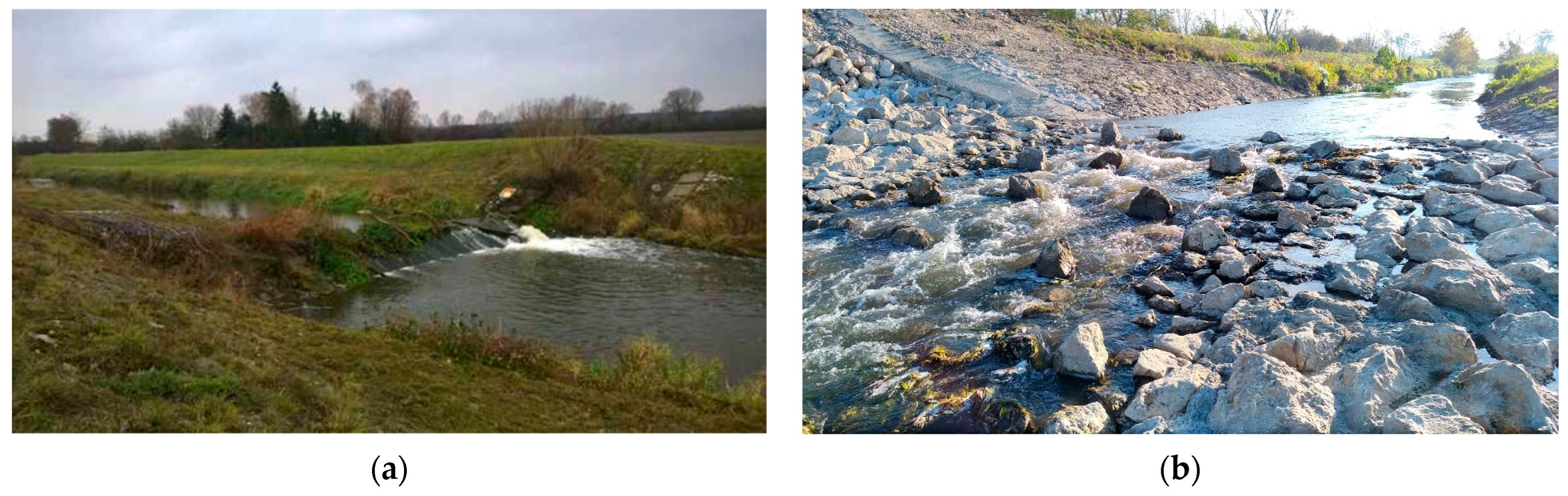
The investigated fish pass, in the form of a ramp (Figure 1), was built on the Myjava River to replace the fixed erosion-control weir in the barbel fish zone. River has the long-term average discharge of Q_a = 2.11 m³∙s⁻¹. For these conditions, the following limits have to be fulfilled for the fish pass [26]:

-

Maximum flow velocity: v_max = 1.2 m∙s⁻¹.

-

Recommended longitudinal slope: i_o,max = 1:100 (1%).

-

Depth in streamline: y_min = 40 cm (by low flow streams 25 cm).

-

Recommended width in water level: B_min = 2 m.

The primary advantage of a full-width rock-ramp, nature-like fish pass lies in its high effectiveness, as it successfully attracts 100% of migrating ichthyofauna to attempt to overcome the barrier. The disadvantage of this type of fish pass is the dependence on stream flows, which closely related to hydrological conditions and seasonal variations. Therefore, the design included a triangular shape for the central part of the ramp, enabling the concentration of even small flows to achieve the recommended parameters of depths and velocities when incorporating boulder elements.

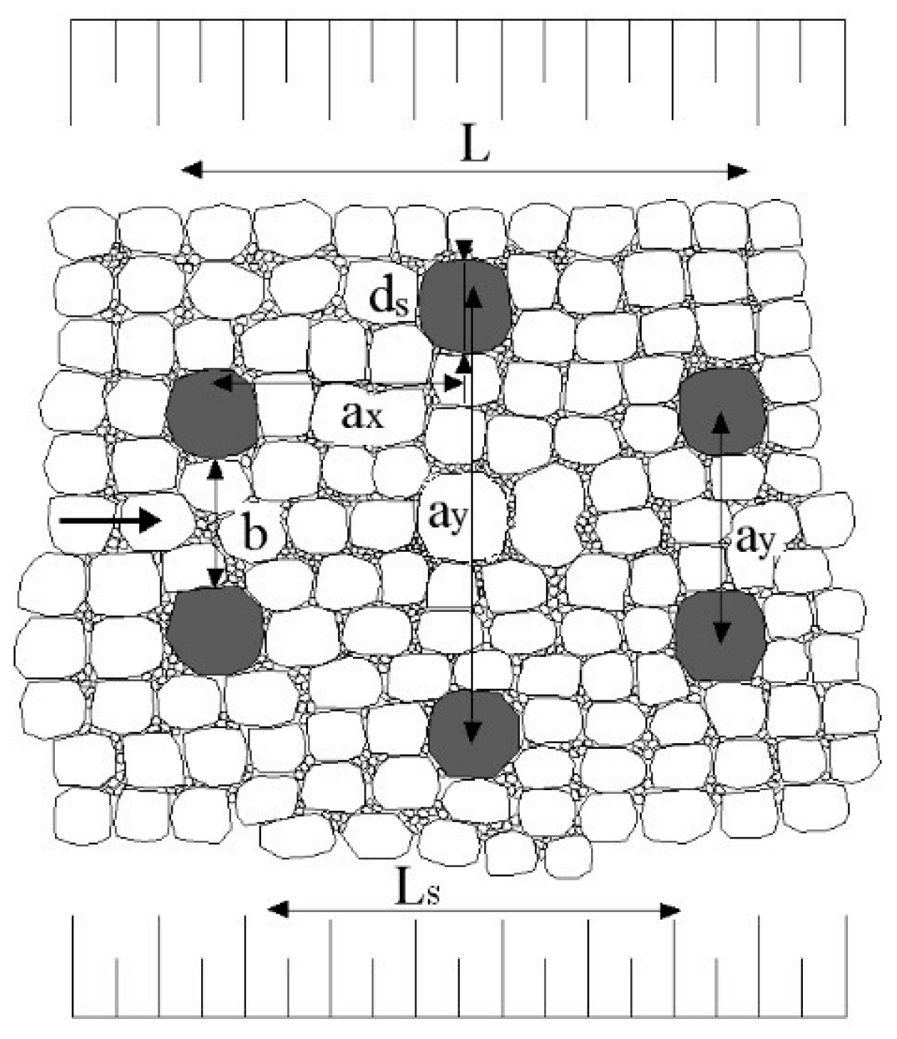
The total length of the investigated fish pass is 19.4 m and it overcomes a head of 0.81 m, which results in a longitudinal slope of i_o = 4.18% or 1:24. The width of the ramp in central triangular-shaped part is 5.8 m; the slope of the banks is 1:7.25. The configuration and placement of boulders is as follows:

-

In 17 profiles, there are 2 boulders chessboard arranged (Figure 2).

-

The dimensions of a single boulder are width x height: 0.3~0.4 m × 0.4 m (mean boulder diameter is d_s = d₅₀ = 0.4 m).

-

In the transverse direction (a_y), the distance a_y = 1.86 m is for the first and the third row of single boulders (from left to right) and a_y = 3.72 m for the second (middle) row of boulders.

-

In the longitudinal direction (a_x), the distance between neighboring profiles with boulders is 1 m.

-

Total number of boulders on ramp is 34.

-

The river bed is created from quarry stones of 20~30 cm placed in concrete and completed by gravel.

Assessment of the boulders according to the different approaches is as follows (parameters are identical to the designation in Figure 2) [17,20]:

a_x = a_y = (1.5 to 3.0, or 5.0)∙d_s

(1)

b = a_y − d_s > 0.3 m

(2)

L = 2∙a_x

(3)

L_s = L − d_s

(4)

Based on the previously described guidelines for boulder arrangements, it can be determined that the longitudinal and transverse distances should fall within the range of a_x = a_y = 0.6–1.2 m (or 2 m) (Equation (1)). However, the arrangement of boulders on the rock ramp is not sufficiently dense. The minimum width distance between boulders, denoted as “b,” is correctly implemented, resulting in an axial distance between boulders, L = 2∙1 = 2 m (Equation (3)). However, the longitudinal clear distances between boulders, denoted as L_s = 2–0.4 = 1.6 m (Equation (4)), fall below the limit specified in

Table 1. Minimum recommended parameters for rock ramps and specific fish species [20].

Fish Species	River Bed		Distances between Boulders
	Depth (m)	Width (m)	Ls (m)	b (m)
Barbel, Zander, Pike, Salmon, and Danubian Salmon	0.5	2.0	3.0	0.4

. According to this evaluation, the number of boulders and their arrangement appear to be inconvenient in terms of limits.

2.2. Roughness Coefficient Determination

The river bed substrate with single boulders creates roughness of the structure, which is substance for the Manning’s roughness coefficient, denoted as “n”, as the basic parameter for the hydraulic calculations. Several methods can be employed to determine the roughness coefficient, including referencing tables that provide descriptions of river bed characteristics, utilizing empirical equations proposed by different authors under specific conditions, employing Cowan’s method, using photographic catalogues, or conducting direct measurements in water courses [27].

Using the mentioned methods for determining the roughness coefficient, a considerable range of values of the roughness coefficient can be obtained. According to the description of the channel for small, natural watercourses (width in water level during floods < 30 m) [23], a mountain-stream-type river bed composed of coarse gravel and large boulders has Manning’s roughness coefficient values of n = 0.040–0.070. The use of, e.g., the empirical Strickler equation [27] (Equation (5)), leads to the following calculation, where “a” is a constant (a = 21.1 for homogeneous sand roughness, a = 24.4 for d = d₅₀) and “d” is a characteristic grain (d = d₅₀ = d_s):

$$n=\frac{1}{\mathrm{a}}{{\mathrm{d}}_{50}}^{1/6}=\frac{1}{24.4}{0.4}^{1/6}=0.035$$

(5)

Cowan’s method expresses the procedure for determining the roughness according to the subjective verbal description of the six characteristic parameters of the river bed (Equation (6)). This method is suitable for small up to medium streams with a hydraulic radius less than 5 m [27]:

$$\begin{gathered} n=\left(n_0+n_1+n_2+n_3+n_4\right){·m}_5=\left(0.030+0.02+0.010+0.02+0.00\right)·1 \\ n=0.080 \end{gathered}$$

(6)

where

• n₀—the influence of the grain size of the substrate (n₀ = 0.028 for coarse gravel; n₀ = 0.030–0.050 for stones);
• n₁—the influence of surface irregularity (n₁ = 0.005 small irregularities (weakly eroded or deepened); n₁ = 0.020 large (eroded banks and rocky asperity));
• n₂—the effect of the variability of the cross section causing turbulence (n₂ = 0.005 occasional changes; n₂ = 0.010–0.015 frequent changes);
• n₃—the influence of obstacles such as trees, boulders, and roots (n₃ = 0.020–0.030 substantial (connection of obstacles that occupy 15–50% of the area); n₃ = 0.040–0.060 strong (obstacles that cover > 50% of the area or cause turbulence on most of the area));
• n₄—the influence of vegetation (n₄ = 0.000 none, or without effect);
• m₅—degree of channel curvature (m₅ = 1.00 small (curvature of 1.0–1.2)).

Based on several provided examples of Manning’s roughness coefficient determination or calculation, it is evident that the coefficient value for the evaluated fish pass ranges from 0.035 to 0.080 (but these values are subjective and the variability of the results can be even higher). The roughness coefficient holds significant importance as a fundamental parameter for subsequent hydraulic calculations in the initial design of nature-like fish passes.

2.3. Field Measurements

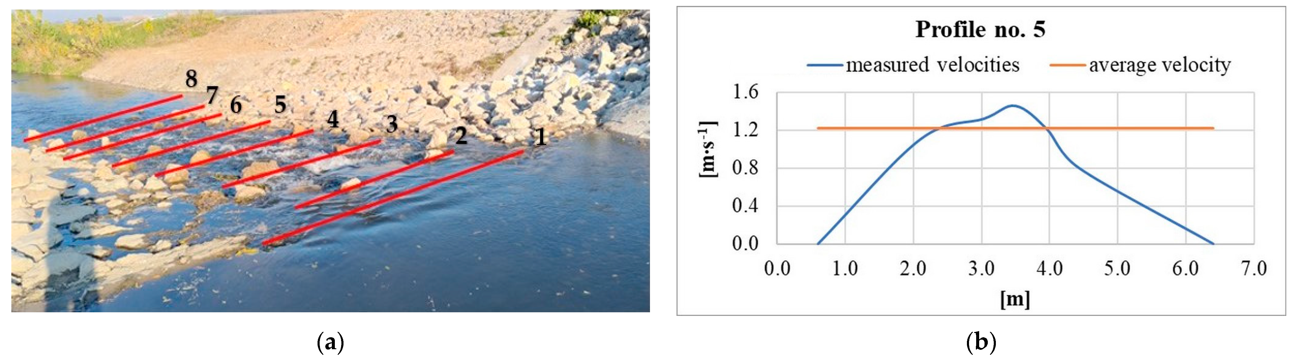
The Water Research Institute conducted field measurements on this fish pass in order to gain real flow velocities for calibration of mathematical models. The velocities were measured in 5 verticals, in 8 profiles (Figure 3), at a low water stage of Q = 0.451 m³∙s⁻¹ (approximately equal to Q₃₃₀). The measurements were conducted during low flow period to verify the passability of the fish pass for low water levels in the stream. Calibrated Universal Current Meter consisting of hydrometric propellers of HYM-type (made by Water Research Institute in Bratislava) was used for the measurements, with a pitch of 0.100 m (according to the standards of fy. A.OTT, type 6). Propellers that were 30 mm in diameter were used. The propellers were combined with a DENTOSAN-type counter with direct evaluation of the measured velocities. HYDRO 11 (Hydrometrics Ltd., Nehvizdy, Czech Republic) was used as the evaluation software.

2.4. Assessment via Numerical models

Based on the previous assumptions, this fish pass was modeled in HEC-RAS 6.3.1 software, both in 1D and 2D environments [28], to verify the fish-pass parameters according to valid national legislation. A 1D model appears to be simpler but has limited results; a 2D model, especially when used to create the geometry, can be quite problematic, but the results are more complex.

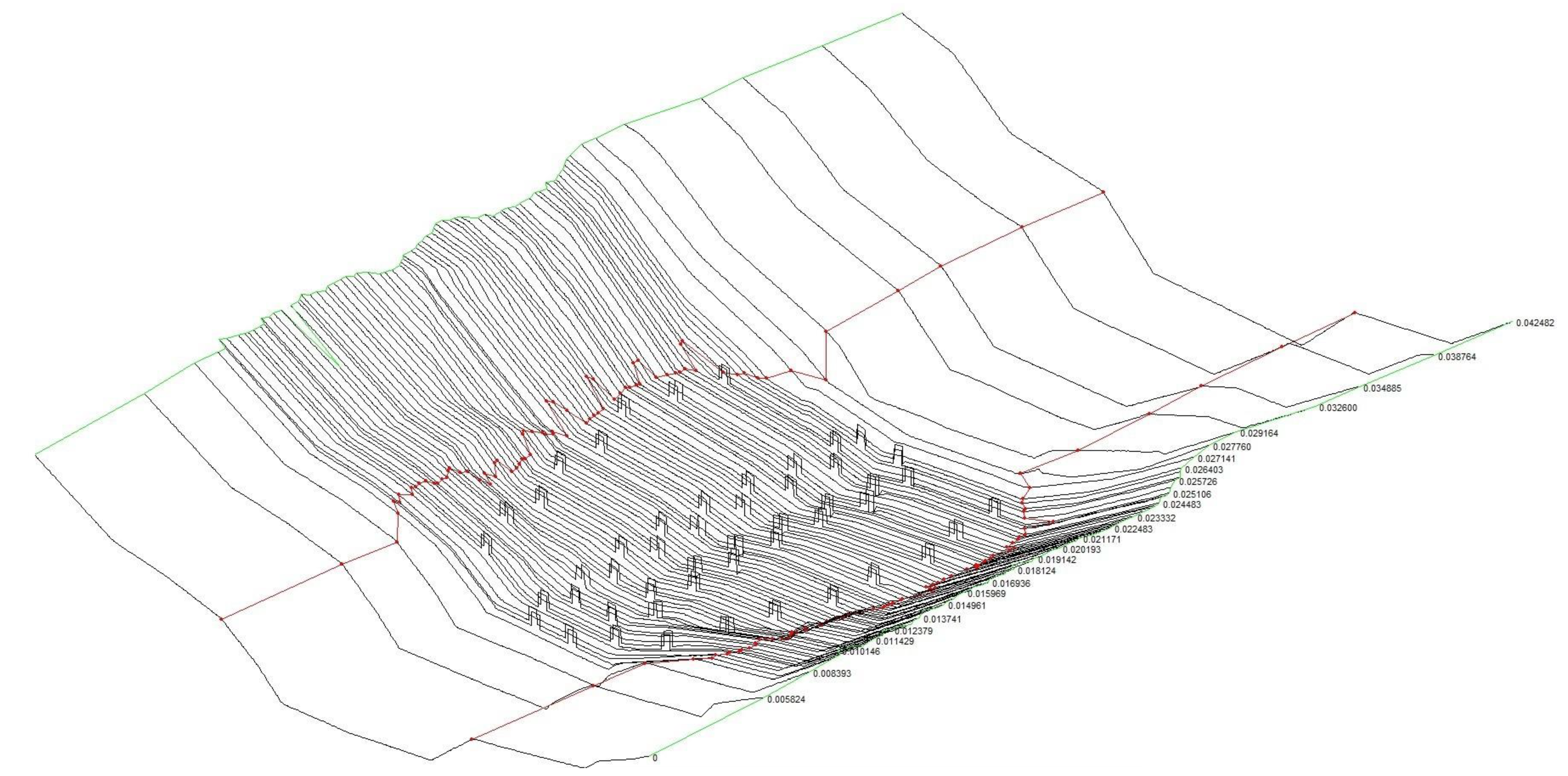
In this case, the geometry for the 1D model was schematized with the help of cross-sections even in the locations of isolated boulders (78 cross-sections were entered on a length of 42.5 m), which meant a large number of profiles were used in order to truly describe each change in geometry along the length of the fish pass (Figure 4).

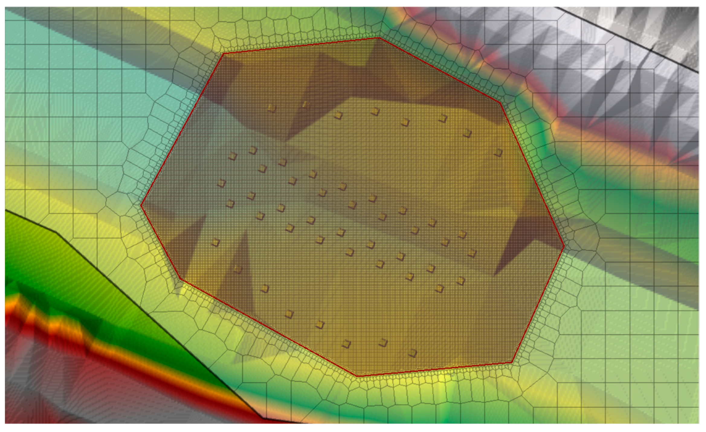
In the case of the 2D model, the decisive criterion was the detail of the computational mesh at the location of the boulders (Figure 5), while keeping the Courant criterion. The limit for the Courant´s number (Equations (7)–(9)) affects both the cell size of the computational mesh as well as the selected computational equation (SWE-ELM (Shallow Water Equations, Eulerian–Lagrangian Method), SWE-EM (Shallow Water Equations, Eulerian Method), or DWE (Diffusion Wave Equations)) [28]:

$$\mathrm{f}\mathrm{o}\mathrm{r} \mathrm{S}\mathrm{W}\mathrm{E}-\mathrm{E}\mathrm{L}\mathrm{M}\mathrm{C}=\frac{\mathrm{v}·\Delta \mathrm{T}}{\Delta \mathrm{x}}\le 1.0 (\mathrm{w}\mathrm{i}\mathrm{t}\mathrm{h} \mathrm{a} \mathrm{m}\mathrm{a}\mathrm{x}.\mathrm{C}=3.0)$$

(7)

$$\mathrm{f}\mathrm{o}\mathrm{r} \mathrm{S}\mathrm{W}\mathrm{E}-\mathrm{E}\mathrm{M}\mathrm{C}=\frac{\mathrm{v}·\Delta \mathrm{T}}{\Delta \mathrm{x}}\le 1.0 (\mathrm{w}\mathrm{i}\mathrm{t}\mathrm{h} \mathrm{a} \mathrm{m}\mathrm{a}\mathrm{x}.\mathrm{C}=1.0)$$

(8)

$$\mathrm{f}\mathrm{o}\mathrm{r} \mathrm{D}\mathrm{W}\mathrm{E}\mathrm{C}=\frac{\mathrm{v}·\Delta \mathrm{T}}{\Delta \mathrm{x}}\le 1.0 (\mathrm{w}\mathrm{i}\mathrm{t}\mathrm{h} \mathrm{a} \mathrm{m}\mathrm{a}\mathrm{x}.\mathrm{C}=5.0)$$

(9)

where

• C—courant number;
• v—velocity (wave celerity) (m∙s⁻¹);
• ΔT—computational time step (s) (minimum ΔT = 0.1 s);
• Δx—average cell size (m).

The equation of motion, the so-called DWE, is used in larger models that do not require a detailed solution of the flow around certain obstacles. It finds its application, for example, in the modeling of open river beds and in the design of flood protection measures. The diffusion wave is practically a simplified dynamic wave, where the approximation consists of neglecting the non-linear term of the inertial force, because it assumes a small change in the flow with increasing time. The dynamic wave is also known as the de Saint-Venant equation, which is used to describe unsteady flow in open models. The basis for the derivation of the Saint-Venant equations was the system of Navier–Stokes equations. The HEC-RAS 2D model uses them in an approximate form, so-called SWE, because negligible vertical velocity components are assumed in 2D flow and that the flowing liquid is incompressible and of constant density. In HEC-RAS, there are two methods for solving the SWE—the Eulerian–Lagrangian Method (the advantage of this approach is that it is stable for large time steps, but it can create excessive numerical diffusion of momentum, leading to inaccurate results in lab-scale simulations where strict conservation of momentum is important) and the Eulerian Method (which is an alternative approach utilizes the momentum-conservative discretization of the acceleration terms) [28,29].

For the simulation of the full-width rock-ramp, nature-like fish pass, the SWE-ELM solver with turbulence was used. The chosen detailed mesh in the area of the fish pass and single boulders had a cell size of 0.1 m, and the river bed above and below the rock ramp had a computational mesh that was less detailed, with cells that were 1.5 m in size. During the measurement of vertical velocities, the maximum velocity of 1.9 m∙s⁻¹ was measured, so it was assumed that the velocity of 2.0 m∙s⁻¹ would not be exceeded during mathematical modeling at low flows. Assuming the selection of the smallest calculation time step ΔT = 0.1 s, the Courant number is C = 2 for a cell with a size of 0.1 m and C = 0.13 for a cell with a size of 1.5 m, thus the condition for the Courant criterion (Equation (7)) is fulfilled.

3. Results

In mathematical modeling, calibration is one of the most important phases, which serves to verify the accuracy of the hydraulic calculations. In this process, a suitable combination of boundary conditions and hydraulic parameters of the model is sought by trial and error.

The only parameter that was changed in the model to achieve values equal or nearly equal to the measured ones was Manning’s roughness coefficient. The process of calibration is the same for both models, 1D and 2D, respectively, but the outputs, which are compared, are the average velocities for the 1D model and the vertical velocities for the 2D model. Different values of Manning´s roughness coefficient from the range n = 0.035~0.080 were used to obtain a calibrated model. Simulation discharge was set at Q = 0.451 m³∙s⁻¹, which is the same value as obtained during measurements.

3.1. Results Obtained via the 1D Model

The 1D model seems to be easier for practical utilization, but for fish-pass modeling, it does not meet the conditions of the flow pattern and velocity field; however, the model can help with the first assessment of the designed structure. The boulders can be incorporated in the model geometry in various forms: as a cross-section geometry (as was modeled in this case), as obstructions in cross-sections, or as fixed weirs with gates. Anyway, each approach requires a very detailed description of each boulder to capture the cross-sectional changes in profiles.

The calibration process was not completely successful due to the previously computed range of Manning´s roughness coefficient. The entire range of n = 0.035~0.080 was used.

Table 2. Comparison of simulated (1-D model) and measured parameters in the solved fish pass.

Profile No.	Measurement		HEC-RAS 1D
	Depth (m)	Velocity (m∙s−1)	Depth (m)	Velocity (m∙s−1)
1	0.28	0.49	0.27	0.52
2	0.22	0.69	0.31	0.61
3	0.22	0.99	0.28	0.77
4	0.23	1.18	0.29	0.72
5	0.30	1.22	0.30	0.69
6	0.30	1.07	0.29	0.75
7	0.32	0.76	0.31	0.65
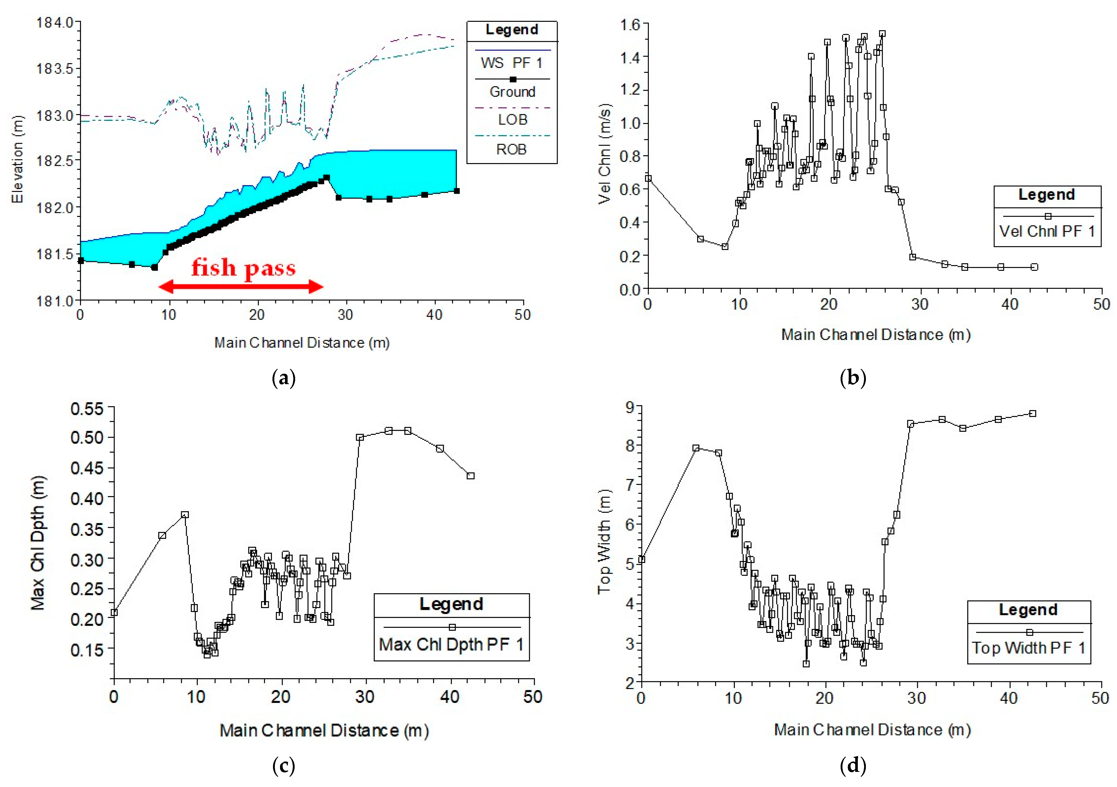
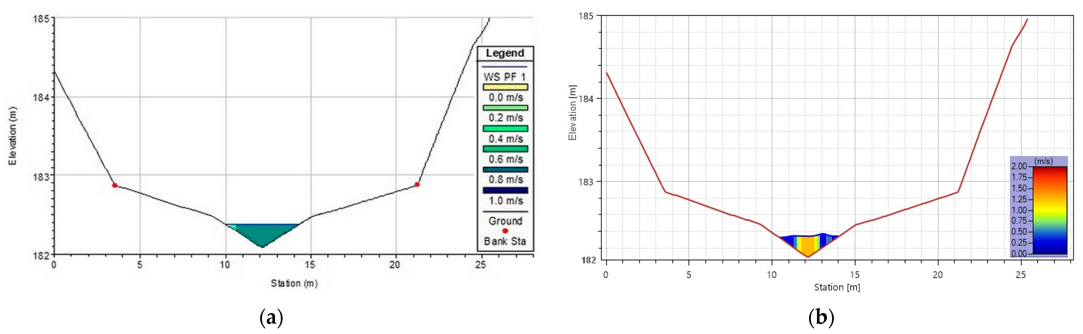
8	0.40	0.48	0.26	0.63

shows the comparison between the measured and modeled values of depths and velocities. It is obvious that the upper section (profiles 1 and 2) of the model shows good compliance with measured velocities, and the rest of the profiles comply only in depth, but the modeled velocities were lower than the measured ones (Table 2, Figure 6a). The achieved values of simulated velocities are in the range of 0.25–1.54 m∙s⁻¹ (the average velocity along the fish pass is 0.88 m∙s⁻¹) (Figure 6b); for depths, they are in the range of 0.14–0.37 m (the average depth is 0.24 m) (Figure 6c), the width at water levels varies between 2.5 m and 7.8 m (the average width is 4 m) (Figure 6d). From the point of view of prescribed limits in the fish pass, the velocities are below the limit (1.2 m∙s⁻¹), the depths are in the limit for lower flows in streams (minimum recommended depth is 25 cm), and the width in the water surface limit is fulfilled in the whole fish-pass environment (the minimum is 2 m).

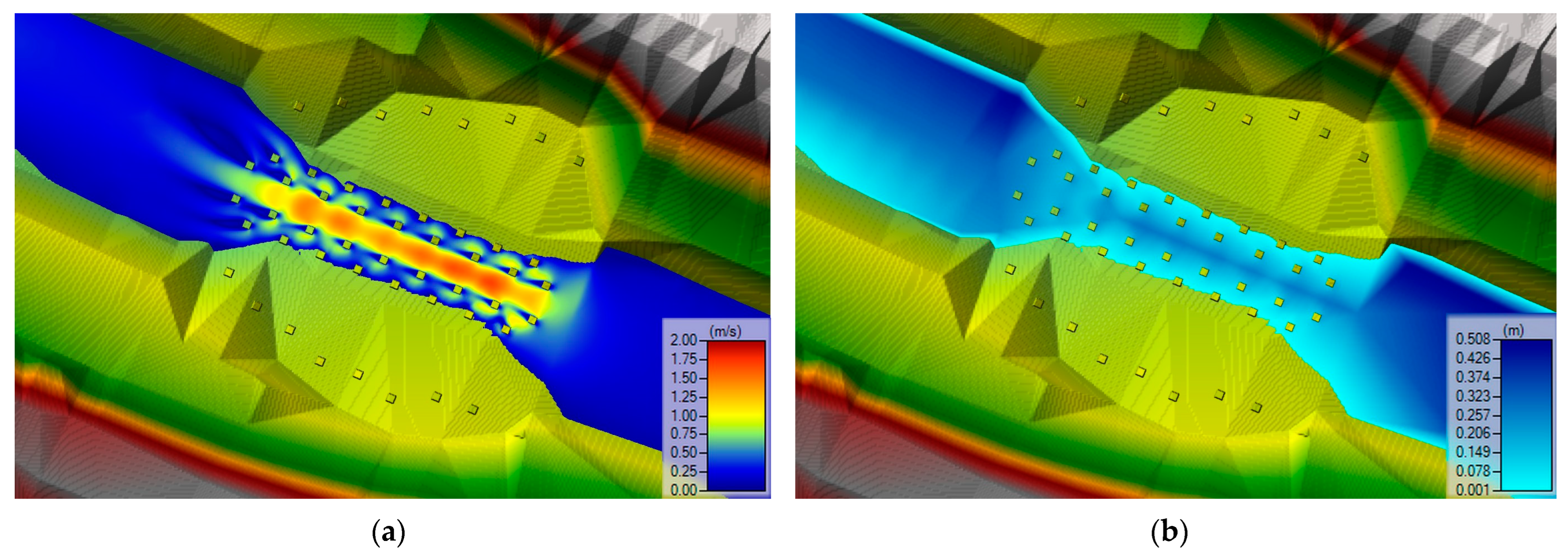
3.2. Results Obtained via the 2D Model

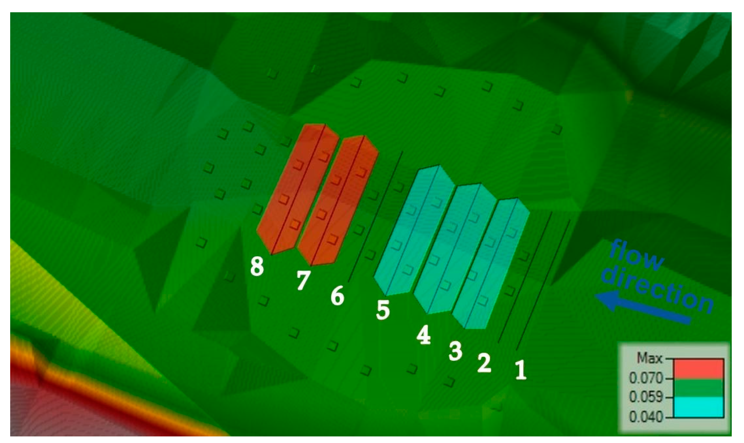
After several simulations with different Manning’s roughness coefficients, the final calibrated model was achieved, where this parameter varied between 0.040 and 0.070 (Figure 7). The calibration was completed, especially in terms of measured vertical velocities in eight cross-sections (Figure 8).

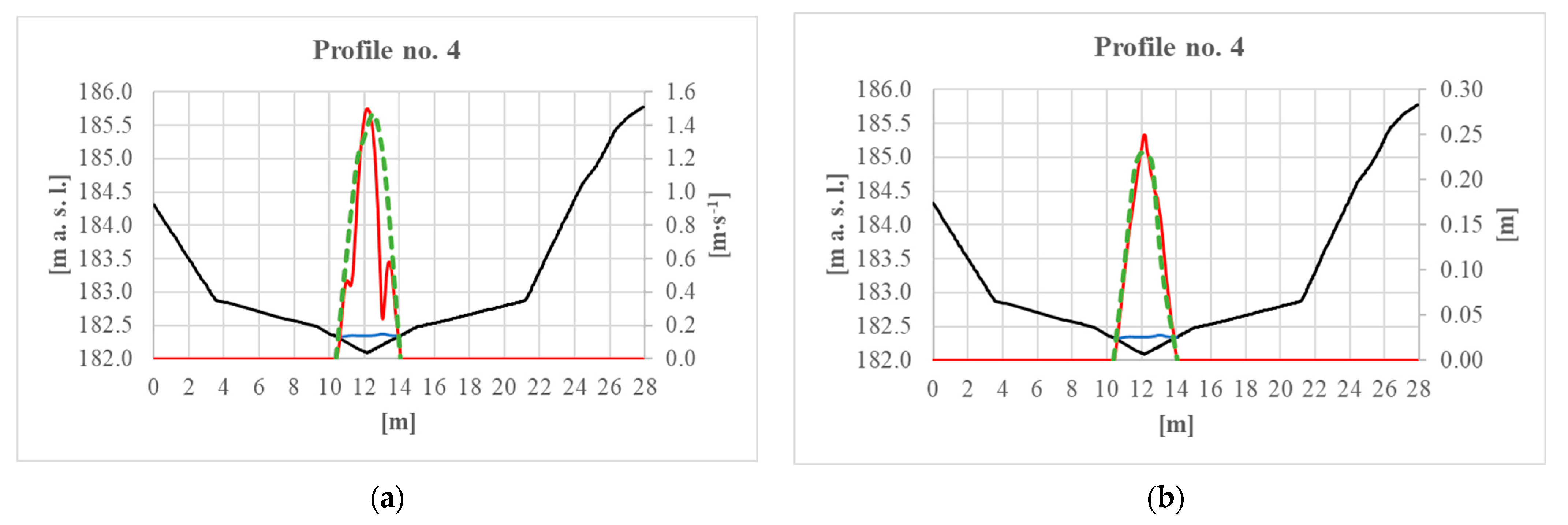
The obtained results from this model show that the fish pass is also passable at low flows in the river (Q = 0.451 m³∙s⁻¹), but the limit for the maximum acceptable flow velocity in the barbel zone is exceeded. The prescribed limit is 1.2 m∙s⁻¹, and the simulated maximum velocity was 1.69 m∙s⁻¹ (Figure 9a). The width of the water level varied from 3.3 m up to 4.1 m, whereas the limit is min. 2 m, so a bigger water environment was created. The depths in the middle part (streamline) of the fish pass were around 0.20~0.29 m (Figure 9b), while the minimum recommended depth was 25 cm by low stages. It can be assumed that such a small discharge in the stream occurs during the summer session, when there is no spawning or significant migration period for the target fish species.

3.3. Comparison of 1D and 2D Model Results

Both models simulated a nature-like fish pass with single boulders. The 1D model gives a rough overview of the depths and velocities, whereas the 2D model describes the velocity field, occurring eddies, and shadows behind the boulders. The ranges of Manning’s roughness coefficients differ. For the 1D model, the whole range (0.035–0.080) of the calculated coefficients was used; for the 2D model, values of 0.040–0.070 were used. Profiles close to measured profile no. 1 in the 1D model have n = 0.070; profiles around measured profiles no. 2, 3, and 4 have n = 0.035; profiles near measured profiles no. 5 and 6 have n = 0.040; profiles close to measured profile no. 7 have n = 0.070; profile no. 8 has n = 0.080, respectively. For the 2D model, the areas with Manning’s roughness coefficient are as follows: area close to the measured profiles no. 1 and 2: n = 0.059; profiles no. 3, 4, and 5: n = 0.040; profile no. 6: n = 0.059; and the area near the measured profiles no. 7 and 8: n = 0.070 (

Table 3. Comparison of Manning’s roughness coefficient used in mathematical models.

Profile No.	Manning’s Roughness Coefficient
	1D Model	2D Model
1	0.070	0.059
2	0.035	0.059
3	0.035	0.040
4	0.035	0.040
5	0.040	0.040
6	0.040	0.059
7	0.070	0.070
8	0.080	0.070

). Manning’s roughness coefficient´s values used in the 2D model seem to be more realistic because n = 0.035 looks too small for such an environment full of large boulders, but n = 0.080 is a value mostly used for inundations or banks heavily overgrown by vegetation.

Velocities in the 1D model were smaller than the measured ones (the maximum velocity was 1.54 m∙s⁻¹); the 2D model (the maximum velocity was 1.69 m∙s⁻¹) better complied with the measured velocities in the profiles, but bigger values also occurred that were measured (Figure 10,

Table 4. Comparison of simulated (2-D model) and measured parameters in the solved fish pass.

Profile No.	Measurement		HEC-RAS 2D
	Depth (m)	Velocity (m∙s−1)	Depth (m)	Velocity (m∙s−1)
1	0.28	0.49	0.27	0.70
2	0.22	0.69	0.29	0.95
3	0.22	0.99	0.27	1.27
4	0.23	1.18	0.25	1.50
5	0.30	1.22	0.26	1.45
6	0.30	1.07	0.27	1.34
7	0.32	0.76	0.28	1.21
8	0.40	0.48	0.23	1.28

).

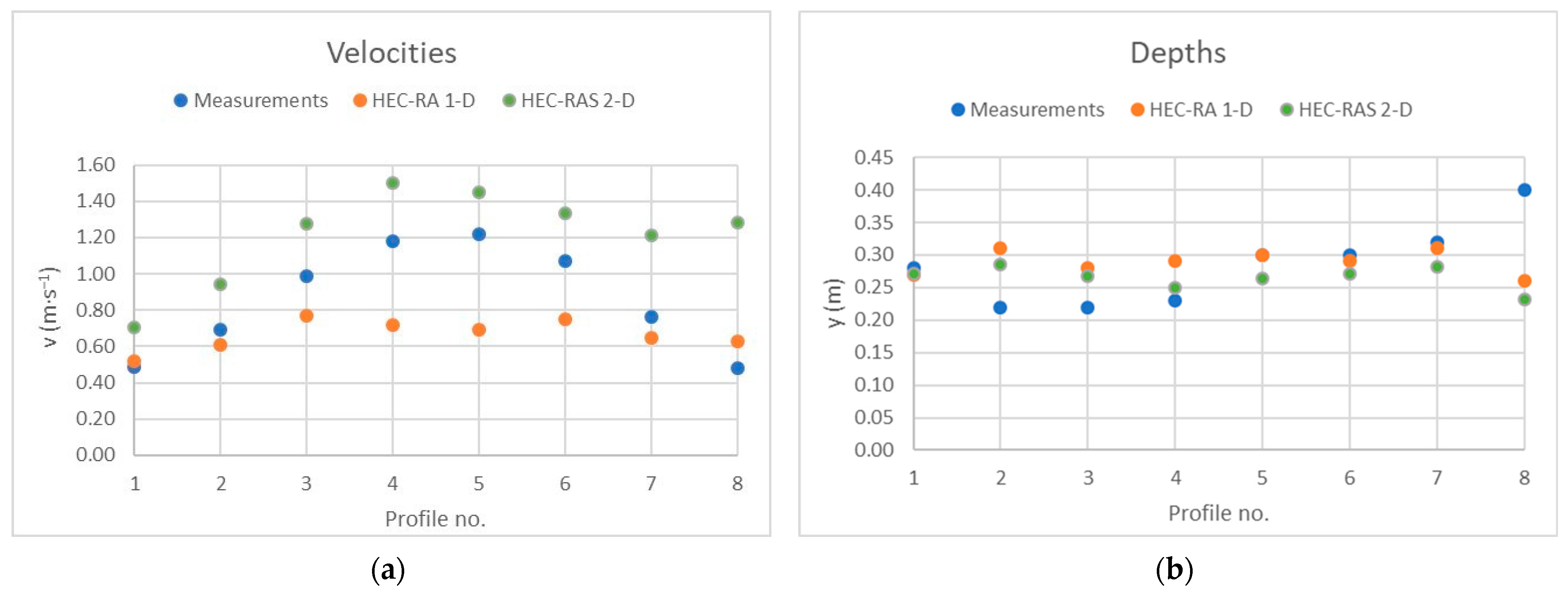
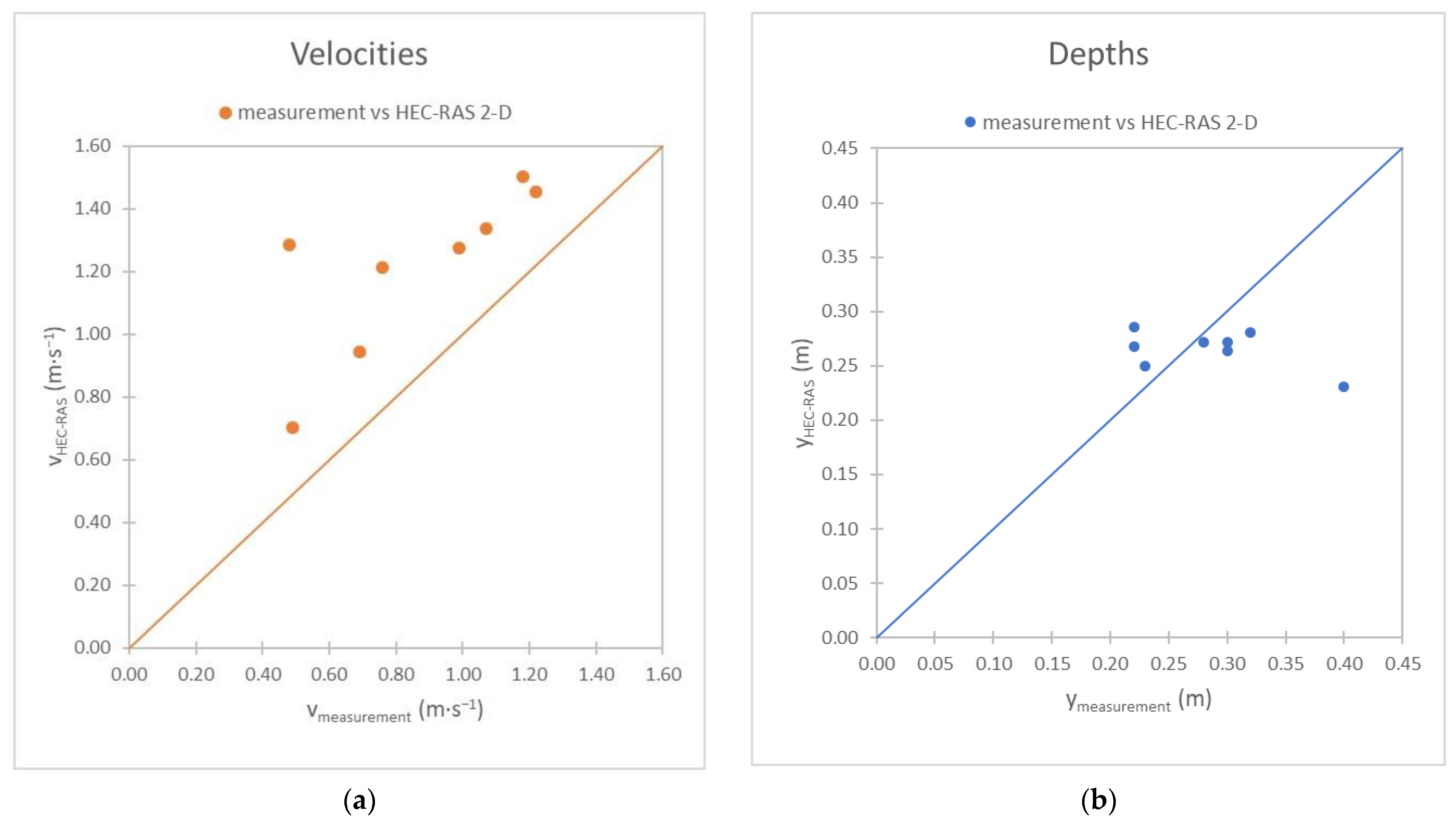
Regarding the achieved depths (range for the 1D model 0.14–0-37 m and the 2D model 0.20–0.28 m, respectively), the results are very similar for both of the models and are very close to the measured values. For a visualization of results (velocities and depths) compared to the measured data, the following graphs (Figure 11) were created, where in profiles with measurements that were also corresponding data from both models were plotted (based on Table 2 and Table 4). Compared to the measured velocity values, the 2D model exceeded the velocities, while the 1D model did not achieve them. Simulated depths from both models are in fairly good compliance when half of the monitored profiles also match the measured depths.

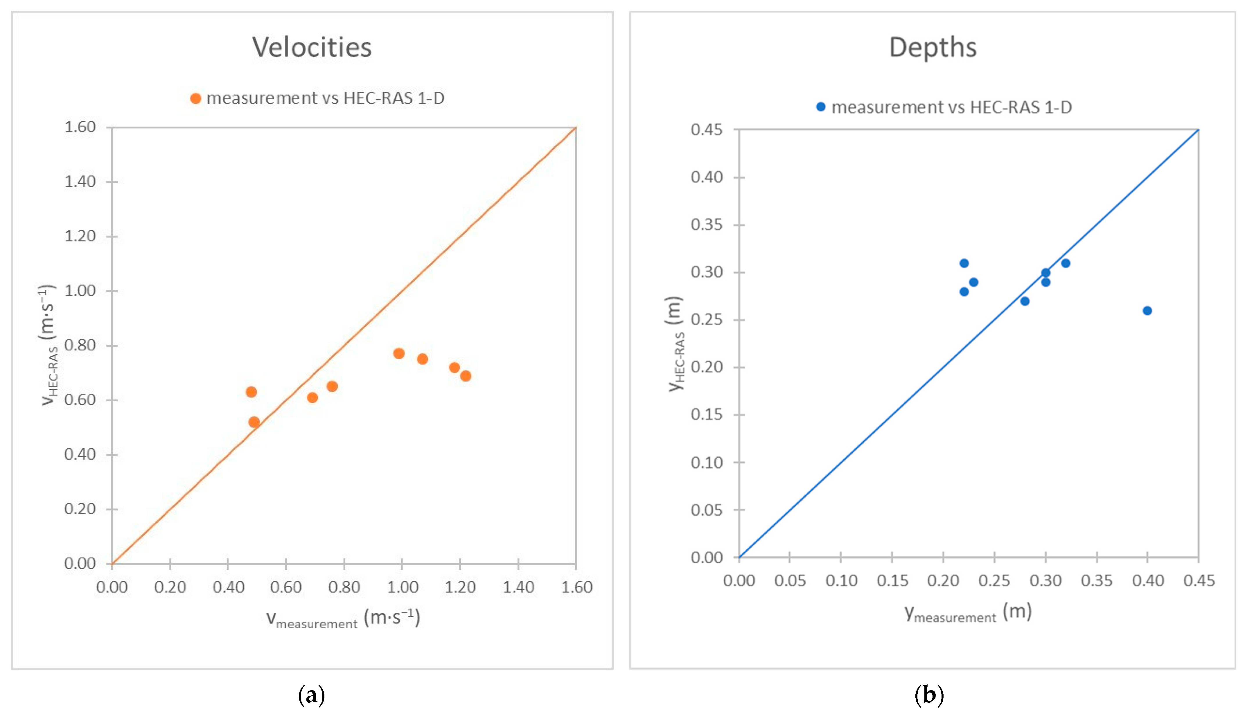
In our study, we conducted an assessment of the HEC RAS 1D model and 2D models by comparing their results to field measurements of the depth and velocity (Figure 12 and Figure 13). We utilized the root mean squared error (RMSE) and mean absolute error (MAE) as metrics to evaluate the accuracy of the models.

For the depth (m) assessment of the 1D model, the RMSE value was 0.0663 and the MAE value was 0.035. These values indicate the average difference between the predicted depth values from the model and the observed field measurements. A smaller RMSE and MAE indicate a better compliance between the model predictions and the actual measurements. In this case, the 1D model demonstrated relatively low errors, suggesting a good accuracy in predicting depth.

Regarding the velocity (m∙s⁻¹) assessment of the 1D model, the RMSE was 0.293 and the MAE was 0.185. Similar to the depth assessment, a smaller RMSE and MAE indicate better accuracy. These values suggest that the 1D model performed reasonably well in predicting velocity, but with slightly higher errors compared to the depth assessment.

Moving on to the 2D models, for the depth (m) assessment, the RMSE was 0.07 and the MAE was 0.0375. These values indicate a slightly higher error compared to the 1D model, suggesting that the 2D models had a slightly lower accuracy in predicting depth.

For the velocity (m∙s⁻¹) assessment in the 2D models, the RMSE was 0.398 and the MAE was 0.274. These values indicate higher errors compared to both the 1D model and the depth assessment in the 2D models, suggesting a less accurate prediction of velocity.

Overall, based on the RMSE and MAE values (

Table 5. Comparison of Error Indices obtained from 1-D and 2-D model results in the solved fish pass.

Error Indices	HEC-RAS 1D		HEC-RAS 2D
	Depth (m)	Velocity (m∙s−1)	Depth (m)	Velocity (m∙s−1)
RMSE	0.0663	0.293	0.070	0.398
MAE	0.0350	0.185	0.0375	0.274

), the 1D model exhibited better performance in predicting both the depth and velocity compared to the 2D models. However, it is important to interpret these values in the context of the specific application and the acceptable level of error. Further analysis and refinement of the models may be required to improve their accuracy and reliability for future assessments.

4. Discussion

The assessed rock-ramp fish pass belongs to the barbel fish zone, which is characterized by a wider range of species than the upper part of the river, a river bed slope of 0.3–0.025%, a water temperature of 12°–18 °C, less oxygenated water, and fine gravel on the river bed. Typical representatives are the common barbel (Barbus barbus), the gudgeon (Gobio gobio), the bleak (Alburnus alburnus), the silver bream (Blicca bjoerkna), and the common nase (Chondrostoma nasus), as well as predatory fish like the northern pike (Esox lucius) and the perch (Perca fluviatilis) [18]. In Slovakia, the middle parts of most of our streams belong to this fish/barbel zone, limited by altitudes of 150–360 m a.s.l. [17].

A comprehensive assessment of the passability of the investigated fish pass requires consideration not only of hydraulic parameters but also of the data derived from an ichthyological survey. Currently in Slovakia, there is no requirement for an ichthyological survey in relation to fish passes that replace removed barriers across the entire width of the stream. The assumption is that 100% of the ichthyofauna will migrate successfully using such fish passes, as there are no alternative routes available [17,18]. However, whether the fish are capable of migrating upstream or if their movement is restricted to downstream migration only remains the crucial question. Consequently, stricter limits are prescribed to ensure close to nature conditions for the migration of species, in this case, from the barbel zone.

Based on the general parameters prescribed for this type of fish pass in Slovakia and abroad in the barbel zone, it can be suggested that migration via fish passes will be successful during the majority of the year, in the migration period (spring and autumn). An assessment of the hydraulic parameters for rock-ramp fish passes is conducted for the range of discharges Q₉₀–Q₃₃₀, where the lower limit represents the Slovakian conditions and autumn migration period (Q₂₇₀–Q₃₃₀) [17]. Therefore, the investigated calibrated model is suitable for simulating the required stages for the prescribed range of discharges.

For the simulated discharge of Q = 0.451 m³∙s⁻¹ ≈ Q₃₃₀ (lower limit of the autumn migration period), assessed parameters are within the required limits, except for the ramp´s slope, which does not need to be achieved when the depths and velocities are suitable (

Table 6. Limits [7,17,18] and achieved parameters in the whole simulated environment of the fish pass.

Parameters	Limits		Results
	Slovakia	Abroad	1D	2D
Longitudinal slope	1:100	1:30~1:20	1:24	1:24
io (-)	(1%)	(3.33~5%)	(4.18%)	(4.18%)
Maximum flow velocity
vmax (m∙s−1)	1.20	1.40	1.54	1.69
Minimum flow depth
ymin (m)	0.40 (0.25) *	0.30~0.40	0.14~0.37	0.2~0.29
Minimum width in water level
Bmin (m)	2	-	2.5~7.8	3.3~4.1

Note: * Limit for low flow period.

).

Despite the statistical evaluation of both models, where the 1D model demonstrates better results than the 2D model, it is important to note that the 1D model significantly simplifies the geometry and neglects the spatial flow patterns around the single boulders. On the other hand, simulations conducted by the 2D model push the boundaries of software capabilities, in terms of computational grid detail and require detailed time step resolution.

5. Conclusions

Making barriers passable is a highly relevant issue that is being addressed by all EU member states because fish migration does not know borders. The theoretical knowledge summarized in methodologies and decrees must be supplemented by continuous field measurements, especially several years after the construction. Of course, it is necessary to correlate the hydraulic parameters with the research of ichthyologists in order to be able to make any adjustments to ensure the highest possible passability of the barriers on the streams.

As shown in this article, the practical procedure of evaluating an existing fish pass according to theoretical recommendations is a long-term process, requiring a large amount of data and the cooperation of several experts from different fields. In the future, on the basis of their evaluation, it will be possible to propose several changes in the design limits of the fish pass so that it meets the prescribed requirements; respectively, it will be the subject of physical model research of complex hydraulic phenomena that occur during the flow of water in the nature-like fish-pass river bed.