
Low-Quality Irrigation Water Treated Using Waste Biofilters

 , ,
, ,  ,
, 
Abstract
1. Introduction
2. Materials and Methods
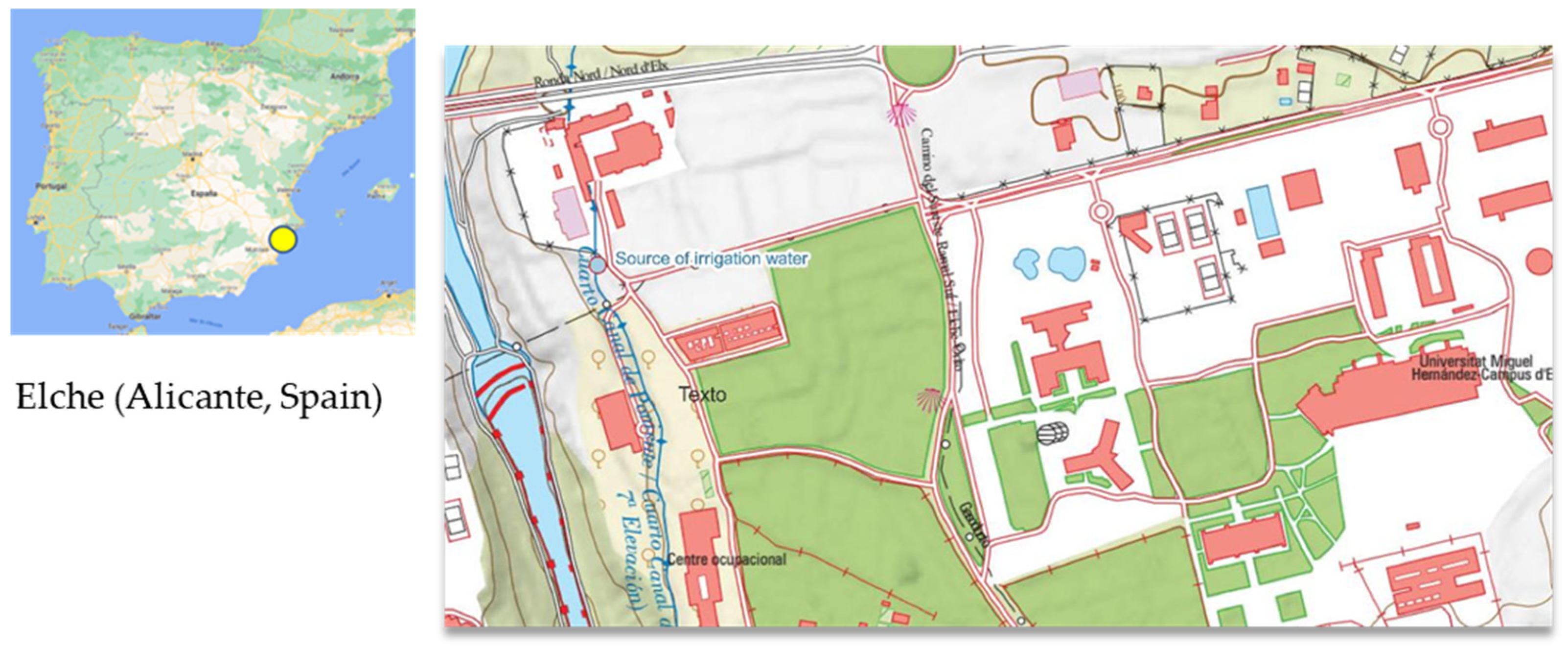
2.1. Irrigation Water Source
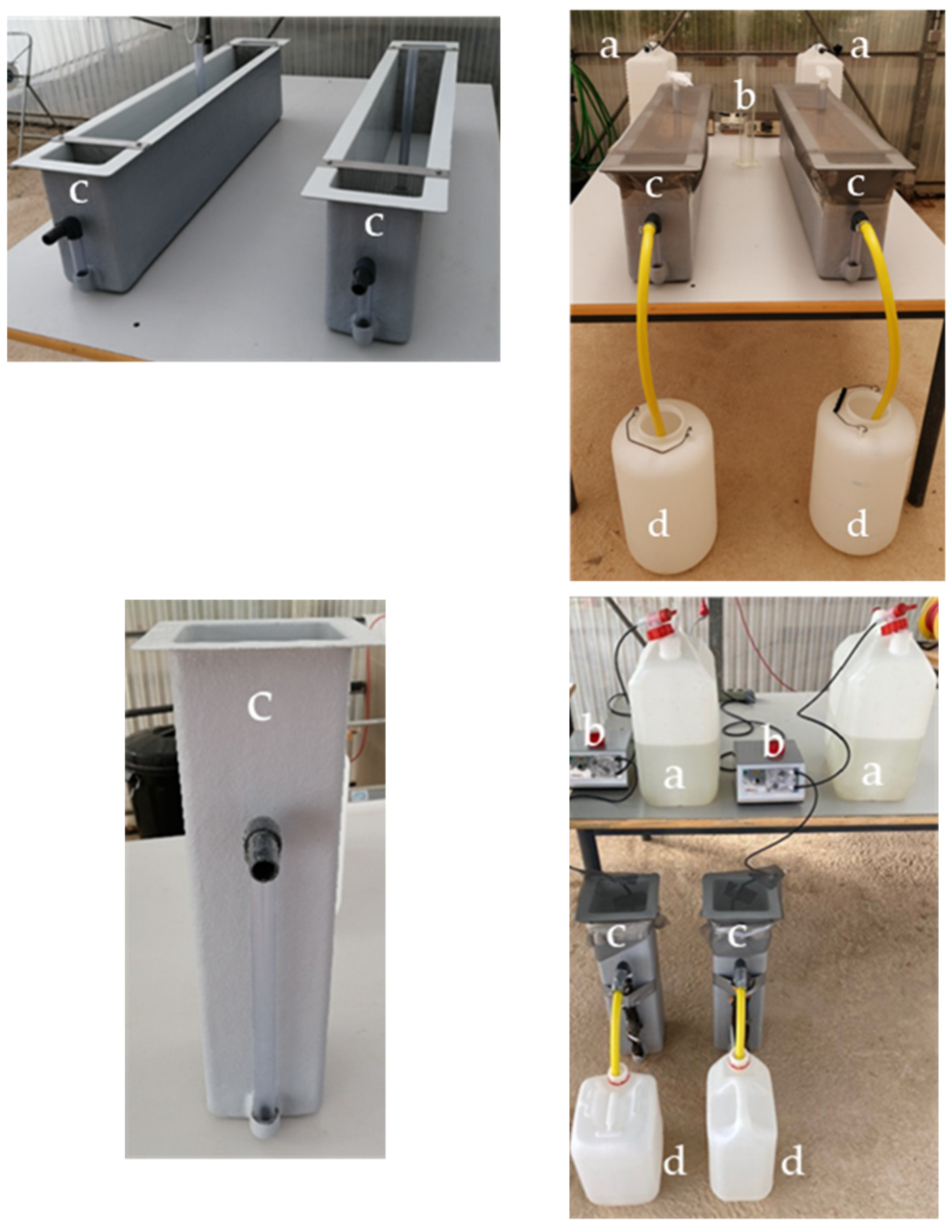
2.2. Bioreactor Designs
- -
- Horizontal water flow with filter of G (HG).
- -
- Horizontal water flow with filter of G and A (HA).
- -
- Vertical water flow with filter of G (VG).
- -
- Vertical water flow with filter of G and A (VA).
2.3. Water Characterization Methods
2.4. Statistical Analysis
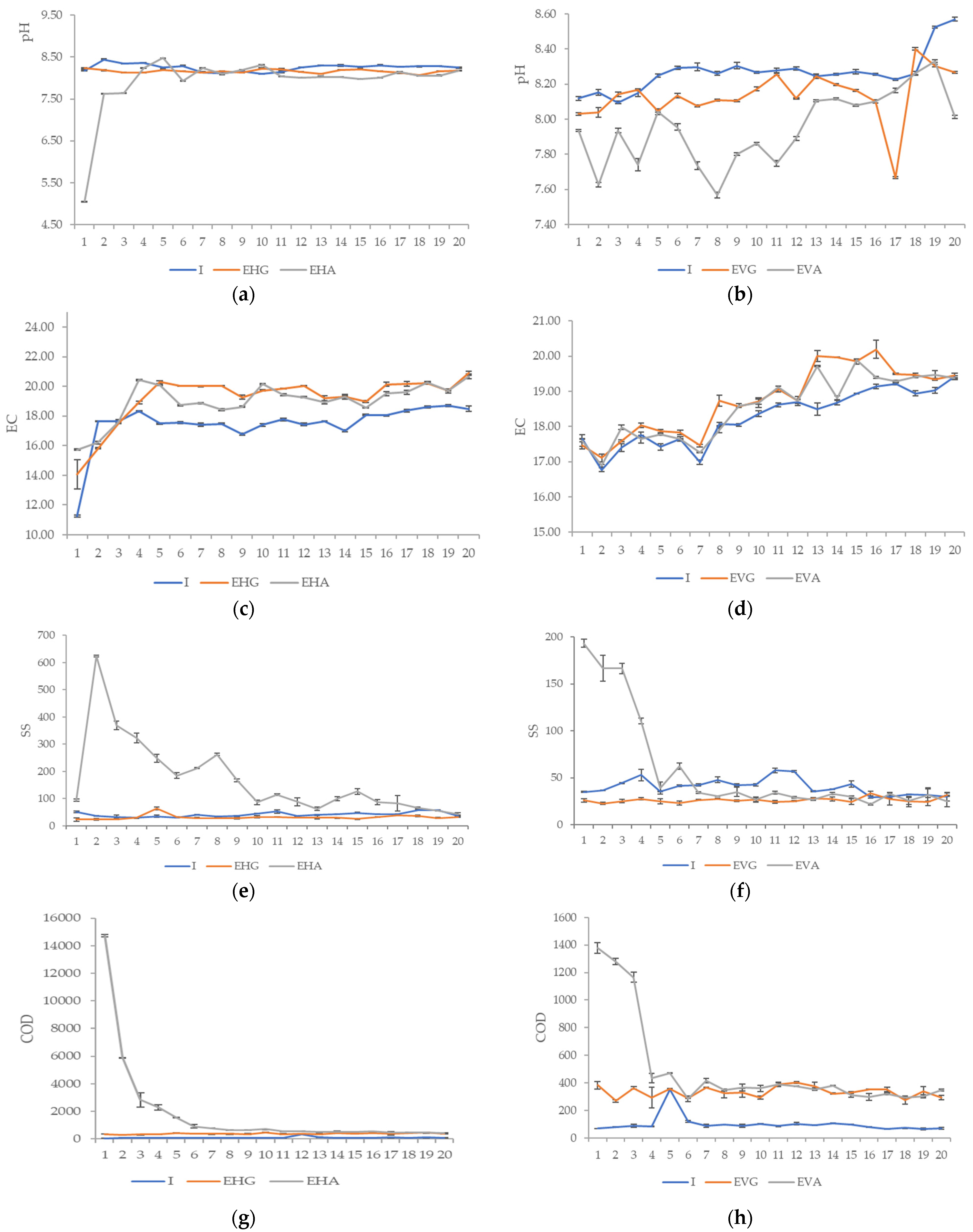
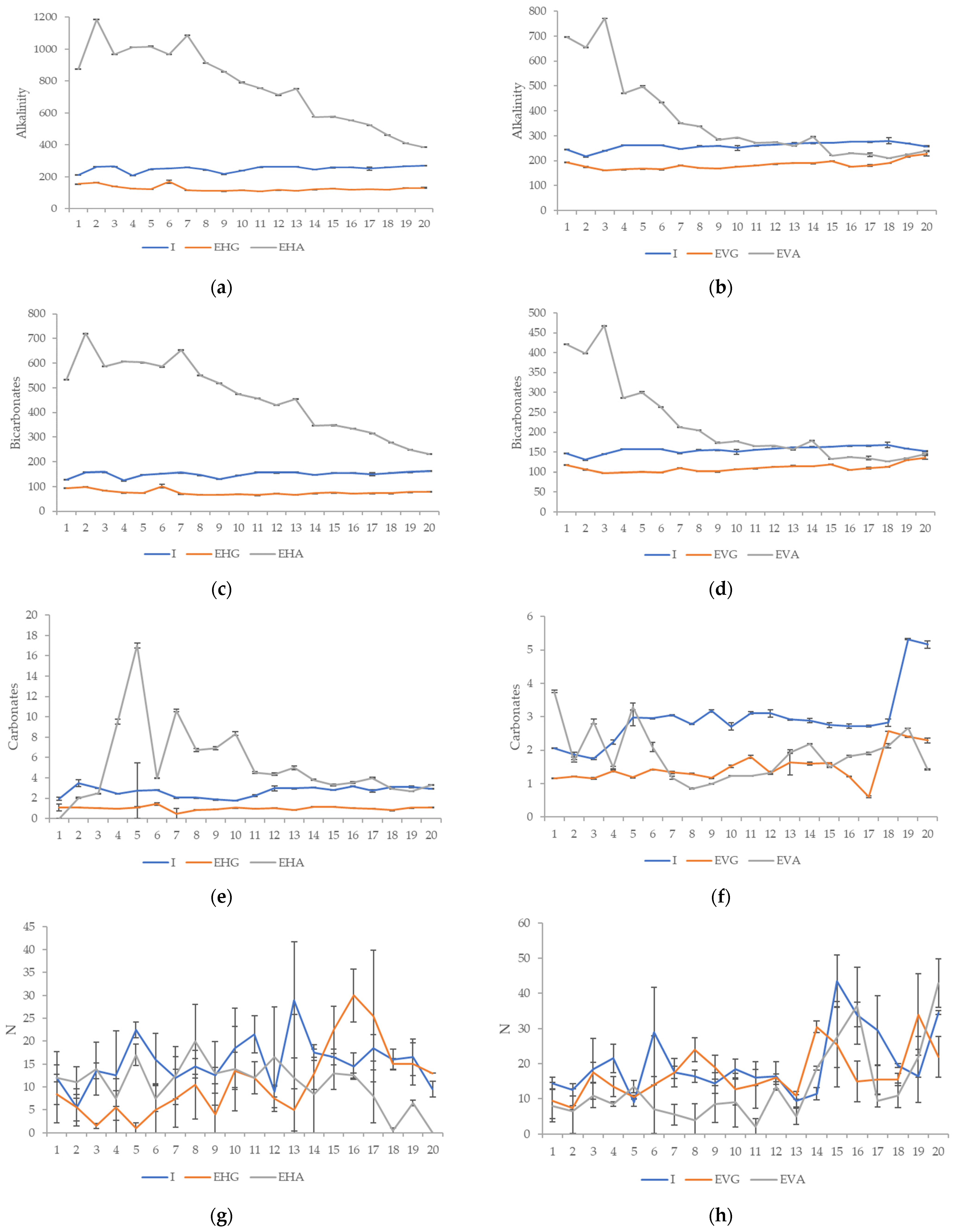
3. Results and Discussion
3.1. Irrigation Water Characterization
3.2. Effluent Characterization
4. Conclusions
Author Contributions
Funding
Data Availability Statement
Acknowledgments
Conflicts of Interest
Appendix A

| Horizontal | Week 1 | Week 2 | Week 3 | Week 4 | Week 5 | Week 6 | Week 7 | Week 8 | Week 9 | Week 10 | ||||||||||
|---|---|---|---|---|---|---|---|---|---|---|---|---|---|---|---|---|---|---|---|---|
| M | SD | M | SD | M | SD | M | SD | M | SD | M | SD | M | SD | M | SD | M | SD | M | SD | |
| I | 8.18 | 0.012 | 8.44 | 0.012 | 8.35 | 0.006 | 8.36 | 0.006 | 8.25 | 0.006 | 8.29 | 0.017 | 8.13 a | 0.012 | 8.12 a | 0.010 | 8.15 | 0.015 | 8.10 | 0.006 |
| EHG | 8.23 | 0.012 | 8.19 | 0.013 | 8.13 | 0.008 | 8.13 | 0.006 | 8.19 | 0.008 | 8.17 | 0.006 | 8.13 a | 0.013 | 8.16 | 0.019 | 8.13 | 0.006 | 8.23 | 0.0010 |
| EHA | 5.06 | 0.006 | 7.62 | 0.008 | 7.64 | 0.008 | 8.24 | 0.006 | 8.48 | 0.006 | 7.93 | 0.006 | 8.24 | 0.006 | 8.09 a | 0.013 | 8.19 | 0.017 | 8.31 | 0.013 |
| F | 1 × 10⁶ *** | 5906 *** | 9400 *** | 1588 *** | 2057 *** | 1100 *** | 133 *** | 19.3 *** | 19.4 *** | 2820 *** | ||||||||||
| Week 11 | Week 12 | Week 13 | Week 14 | Week 15 | Week 16 | Week 17 | Week 18 | Week 19 | Week 20 | |||||||||||
| I | 8.15 | 0.021 | 8.25 | 0.010 | 8.29 | 0.010 | 8.30 | 0.021 | 8.26 | 0.012 | 8.31 | 0.017 | 8.27 | 0.006 | 8.28 | 0.013 | 8.29 | 0.0010 | 8.25 | 0.013 |
| EHG | 8.21 | 0.019 | 8.15 | 0.006 | 8.11 | 0.006 | 8.19 | 0.005 | 8.21 | 0.005 | 8.17 | 0.006 | 8.12 a | 0.021 | 8.08 | 0.006 | 8.16 | 0.006 | 8.18 a | 0.005 |
| EHA | 8.04 | 0.006 | 8.01 | 0.008 | 8.03 | 0.017 | 8.03 | 0.005 | 7.98 | 0.006 | 8.01 | 0.008 | 8.14 a | 0.008 | 8.05 | 0.008 | 8.06 | 0.008 | 8.18 a | 0.008 |
| F | 119 *** | 888 *** | 532 *** | 466 *** | 1440 *** | 653 *** | 138 *** | 723 *** | 817 *** | 63.0 *** | ||||||||||
| Vertical | Week 1 | Week 2 | Week 3 | Week 4 | Week 5 | Week 6 | Week 7 | Week 8 | Week 9 | Week 10 | ||||||||||
| M | SD | M | SD | M | SD | M | SD | M | SD | M | SD | M | SD | M | SD | M | SD | M | SD | |
| I | 8.12 | 0.010 | 8.15 | 0.015 | 8.10 | 0.006 | 8.15 a | 0.021 | 8.25 | 0.010 | 8.29 | 0.010 | 8.30 | 0.021 | 8.26 | 0.012 | 8.31 | 0.017 | 8.27 | 0.006 |
| EVG | 8.03 | 0.008 | 8.04 | 0.029 | 8.14 | 0.013 | 8.17 a | 0.005 | 8.05 a | 0.006 | 8.14 | 0.013 | 8.08 | 0.006 | 8.11 | 0.005 | 8.11 | 0.006 | 8.17 | 0.010 |
| EVA | 7.94 | 0.006 | 7.63 | 0.013 | 7.94 | 0.013 | 7.74 | 0.036 | 8.04 a | 0.017 | 7.96 | 0.017 | 7.74 | 0.021 | 7.57 | 0.017 | 7.80 | 0.008 | 7.86 | 0.008 |
| F | 522 *** | 759 *** | 396 *** | 407 *** | 399 *** | 613 *** | 1080 *** | 3531 *** | 1940 *** | 2820 *** | ||||||||||
| Week 11 | Week 12 | Week 13 | Week 14 | Week 15 | Week 16 | Week 17 | Week 18 | Week 19 | Week 20 | |||||||||||
| I | 8.28 a | 0.013 | 8.29 | 0.010 | 8.25 a | 0.013 | 8.26 | 0.006 | 8.27 | 0.012 | 8.26 | 0.006 | 8.23 | 0.006 | 8.26 a | 0.010 | 8.53 | 0.006 | 8.57 | 0.012 |
| EVG | 8.26 a | 0.006 | 8.12 | 0.005 | 8.25 a | 0.006 | 8.20 | 0.006 | 8.16 | 0.005 | 8.10 a | 0.008 | 7.67 | 0.006 | 8.40 | 0.006 | 8.31 | 0.006 | 8.27 | 0.006 |
| EVA | 7.75 | 0.017 | 7.89 | 0.012 | 8.11 | 0.006 | 8.12 | 0.006 | 8.08 | 0.005 | 8.10 a | 0.008 | 8.17 | 0.013 | 8.26 a | 0.008 | 8.33 | 0.008 | 8.01 | 0.010 |
| F | 2230 *** | 1909 *** | 336 *** | 592 *** | 609 *** | 577 *** | 4862 *** | 264 *** | 1309 *** | 3620 *** |
| Horizontal | Week 1 | Week 2 | Week 3 | Week 4 | Week 5 | Week 6 | Week 7 | Week 8 | Week 9 | Week 10 | ||||||||||
|---|---|---|---|---|---|---|---|---|---|---|---|---|---|---|---|---|---|---|---|---|
| M | SD | M | SD | M | SD | M | SD | M | SD | M | SD | M | SD | M | SD | M | SD | M | SD | |
| I | 11.27 | 0.059 | 17.65 | 0.008 | 17.64 | 0.099 | 18.32 | 0.046 | 17.50 | 0.039 | 17.54 | 0.072 | 17.42 | 0.101 | 17.48 | 0.064 | 16.77 | 0.061 | 17.4 | 0.102 |
| EHG | 14.07 | 0.993 | 15.82 | 0.045 | 17.53 | 0.021 | 18.91 | 0.078 | 20.29 | 0.085 | 20.04 | 0.008 | 20.02 | 0.055 | 20.01 | 0.025 | 19.27 | 0.148 | 19.73 | 0.041 |
| EHA | 15.73 | 0.047 | 16.20 | 0.084 | 17.58 | 0.015 | 20.44 | 0.048 | 20.08 | 0.029 | 18.73 | 0.051 | 18.88 | 0.050 | 18.42 | 0.070 | 18.63 | 0.057 | 20.15 | 0.058 |
| F | 5455 *** | 1219 *** | 3.80 ns | 1357 *** | 3018 *** | 2397 *** | 1303 *** | 1518 *** | 702 *** | 1703 *** | ||||||||||
| Week 11 | Week 12 | Week 13 | Week 14 | Week 15 | Week 16 | Week 17 | Week 18 | Week 19 | Week 20 | |||||||||||
| I | 17.76 | 0.078 | 17.42 | 0.095 | 17.64 | 0.024 | 16.99 | 0.070 | 18.07 | 0.043 | 18.05 | 0.034 | 18.37 | 0.086 | 18.62 | 0.056 | 18.71 | 0.053 | 18.49 | 0.176 |
| EHG | 19.84 | 0.028 | 20.03 | 0.019 | 19.20 | 0.177 | 19.30 a | 0.061 | 18.99 | 0.081 | 20.14 | 0.140 | 20.16 | 0.158 | 20.23 a | 0.096 | 19.70 a | 0.141 | 20.90 a | 0.141 |
| EHA | 19.43 | 0.083 | 19.26 | 0.049 | 18.93 | 0.119 | 19.28 a | 0.161 | 18.57 | 0.010 | 19.53 | 0.140 | 19.60 | 0.148 | 20.28 a | 0.050 | 19.73 a | 0.054 | 20.68 a | 0.150 |
| F | 1059 *** | 1280 *** | 180 *** | 620 *** | 300 *** | 345 *** | 206 *** | 725 *** | 161 *** | 289 *** | ||||||||||
| Vertical | Week 1 | Week 2 | Week 3 | Week 4 | Week 5 | Week 6 | Week 7 | Week 8 | Week 9 | Week 10 | ||||||||||
| M | SD | M | SD | M | SD | M | SD | M | SD | M | SD | M | SD | M | SD | M | SD | M | SD | |
| I | 17.65 | 0.008 | 16.77 a | 0.061 | 17.40 | 0.102 | 17.76 a | 0.078 | 17.42 | 0.095 | 17.64 a | 0.024 | 16.99 | 0.070 | 18.07 a | 0.043 | 18.05 | 0.034 | 18.37 | 0.086 |
| EVG | 17.47 | 0.108 | 17.11 | 0.107 | 17.60 | 0.021 | 18.04 | 0.067 | 17.87 a | 0.041 | 17.84 | 0.070 | 17.46 | 0.031 | 18.73 | 0.154 | 18.56 a | 0.015 | 18.71 a | 0.069 |
| EVA | 17.60 | 0.166 | 16.89 a | 0.033 | 17.98 | 0.067 | 17.64 a | 0.109 | 17.77 a | 0.010 | 17.65 a | 0.057 | 17.27 | 0.013 | 17.90 a | 0.087 | 18.59 a | 0.054 | 18.67 a | 0.139 |
| F | 1.45 ns | 21.2 *** | 68.0 *** | 22.4 *** | 61.7 *** | 16.8 *** | 112 *** | 69.5 *** | 259 *** | 13.1 ** | ||||||||||
| Week 11 | Week 12 | Week 13 | Week 14 | Week 15 | Week 16 | Week 17 | Week 18 | Week 19 | Week 20 | |||||||||||
| I | 18.62 | 0.056 | 18.71 | 0.053 | 18.49 | 0.176 | 18.69 | 0.062 | 18.94 | 0.017 | 19.14 a | 0.065 | 19.21 | 0.026 | 18.95 | 0.070 | 19.03 | 0.083 | 19.41 | 0.039 |
| EVG | 19.06 a | 0.080 | 18.73 | 0.125 | 20.00 | 0.164 | 19.96 | 0.008 | 19.85 a | 0.071 | 20.19 a | 0.257 | 19.50 | 0.025 | 19.47 a | 0.048 | 19.34 a | 0.031 | 19.45 | 0.062 |
| EVA | 19.12 a | 0.042 | 18.73 | 0.053 | 19.72 | 0.021 | 18.82 | 0.050 | 19.90 a | 0.019 | 19.40 | 0.031 | 19.29 | 0.026 | 19.42 a | 0.026 | 19.48 a | 0.124 | 19.39 | 0.057 |
| F | 79.6 *** | 0.16 ns | 133 *** | 923 *** | 611 *** | 50.7 *** | 134 *** | 124 *** | 27.4 *** | 1.36 ns |
| Horizontal | Week 1 | Week 2 | Week 3 | Week 4 | Week 5 | Week 6 | Week 7 | Week 8 | Week 9 | Week 10 | ||||||||||
|---|---|---|---|---|---|---|---|---|---|---|---|---|---|---|---|---|---|---|---|---|
| M | SD | M | SD | M | SD | M | SD | M | SD | M | SD | M | SD | M | SD | M | SD | M | SD | |
| I | 51.96 | 3.18 | 35.64 | 1.14 | 31.31 a | 8.29 | 29.49 a | 2.69 | 35.13 | 4.47 | 30.78 a | 2.55 | 41.08 | 0.88 | 34.98 | 0.84 | 36.7 | 0.07 | 44.55 | 0.58 |
| EHG | 23.50 | 6.18 | 24.39 | 3.22 | 24.43 a | 2.36 | 29.43 a | 0.05 | 63.24 | 5.17 | 31.66 a | 0.40 | 28.52 | 1.92 | 28.31 | 2.18 | 28.63 | 2.74 | 33.26 | 4.44 |
| EHA | 94.08 | 3.57 | 624.00 | 2.31 | 369.56 | 15.90 | 322.65 | 18.07 | 248.39 | 14.47 | 184.44 | 10.90 | 212.05 | 1.88 | 262.69 | 4.60 | 166.78 | 4.63 | 86.24 | 8.68 |
| F | 248 *** | 82,946 *** | 1431 *** | 1030 *** | 629 *** | 748 *** | 15,774 *** | 8098 *** | 2491 *** | 98.0 *** | ||||||||||
| Week 11 | Week 12 | Week 13 | Week 14 | Week 15 | Week 16 | Week 17 | Week 18 | Week 19 | Week 20 | |||||||||||
| I | 53.12 | 6.22 | 35.60 a | 0.79 | 41.64 | 0.73 | 42.39 | 1.13 | 47.99 | 2.93 | 42.42 a | 1.05 | 42.55 a | 1.01 | 57.98 | 2.55 | 56.73 a | 1.03 | 35.67 a | 0.55 |
| EHG | 32.09 | 1.07 | 30.25 a | 0.84 | 30.65 | 6.28 | 29.27 | 0.11 | 25.35 | 1.59 | 32.68 a | 0.18 | 39.29 a | 0.34 | 37.05 | 2.80 | 28.70 | 2.44 | 32.91 a | 0.29 |
| EHA | 113.90 | 2.62 | 88.28 | 14.10 | 62.22 | 6.80 | 99.30 | 6.81 | 126.11 | 10.89 | 86.68 | 9.87 | 82.39 | 27.97 | 66.58 | 2.12 | 55.75 a | 0.58 | 43.58 | 4.95 |
| F | 464 *** | 61.7 *** | 35.8 *** | 349 *** | 258 *** | 101 *** | 8.82 ** | 147 *** | 412 *** | 14.8 *** | ||||||||||
| Vertical | Week 1 | Week 2 | Week 3 | Week 4 | Week 5 | Week 6 | Week 7 | Week 8 | Week 9 | Week 10 | ||||||||||
| M | SD | M | SD | M | SD | M | SD | M | SD | M | SD | M | SD | M | SD | M | SD | M | SD | |
| I | 34.98 | 0.69 | 36.70 a | 0.07 | 44.55 | 0.58 | 53.12 | 6.22 | 35.60 a | 0.79 | 41.64 | 0.73 | 42.39 | 1.13 | 47.99 | 2.93 | 42.42 | 1.05 | 42.55 | 1.01 |
| EVG | 25.97 | 1.69 | 22.82 a | 1.06 | 25.18 | 1.88 | 27.67 | 1.30 | 25.06 | 2.66 | 23.04 | 2.27 | 26.34 | 0.67 | 27.60 a | 0.58 | 25.51 | 1.07 | 26.90 a | 2.67 |
| EVA | 193.26 | 4.25 | 205.36 | 13.72 | 166.57 | 5.44 | 110.58 | 2.95 | 39.31 a | 6.50 | 62.54 | 3.45 | 34.39 | 0.84 | 30.62 a | 0.50 | 35.01 | 4.82 | 26.93 a | 1.99 |
| F | 4967 *** | 655 *** | 2109 *** | 441 *** | 13.1 ** | 266 *** | 318 *** | 158 *** | 33.9 *** | 80.7 *** | ||||||||||
| Week 11 | Week 12 | Week 13 | Week 14 | Week 15 | Week 16 | Week 17 | Week 18 | Week 19 | Week 20 | |||||||||||
| I | 57.98 | 2.55 | 56.73 | 1.03 | 35.67 | 0.55 | 37.93 | 0.20 | 43.64 | 3.34 | 29.37 | 1.18 | 30.02 a | 1.42 | 32.43 | 0.28 | 31.92 a | 7.47 | 29.89 a | 4.43 |
| EVG | 24.25 | 1.63 | 25.22 | 0.51 | 27.86 a | 1.32 | 27.68 | 2.11 | 24.41 | 3.08 | 33.29 | 2.36 | 27.53 a | 6.24 | 24.72 a | 5.45 | 24.54 a | 4.28 | 31.88 a | 1.92 |
| EVA | 34.15 | 1.47 | 29.19 | 0.94 | 27.08 a | 0.87 | 33.25 | 1.44 | 29.82 | 1.29 | 22.07 | 0.91 | 32.95 a | 1.61 | 25.34 a | 3.64 | 31.83 a | 6.36 | 25.18 a | 5.98 |
| F | 318 *** | 1598 *** | 96.9 *** | 48.1 *** | 52.8 *** | 50.1 *** | 2.03 ns | 5.11 * | 1.88 ns | 2.4 ns |
| Horizontal | Week 1 | Week 2 | Week 3 | Week 4 | Week 5 | Week 6 | Week 7 | Week 8 | Week 9 | Week 10 | ||||||||||
|---|---|---|---|---|---|---|---|---|---|---|---|---|---|---|---|---|---|---|---|---|
| M | SD | M | SD | M | SD | M | SD | M | SD | M | SD | M | SD | M | SD | M | SD | M | SD | |
| I | 43 | 5.20 | 80 | 3.77 | 67 a | 10.11 | 72 | 6.35 | 70 | 2.31 | 80 | 0.00 | 75 | 1.73 | 69 | 0.01 | 81 | 1.73 | 89 | 10.97 |
| EHG | 338 | 0.02 | 306 | 0.01 | 335 a | 0.82 | 342 | 15.84 | 426 | 22.00 | 381 | 15.01 | 365 | 10.81 | 369 | 36.37 | 358 | 24.54 | 461 | 30.60 |
| EHA | 14,731 | 94.37 | 5901 | 16.52 | 2841 | 515.40 | 2280 | 208.01 | 1556 | 35.22 | 919 | 121.25 | 783 | 0.01 | 653 | 12.73 | 636 | 4.04 | 718 | 2.50 |
| F | 94,705 *** | 4.5 × 10⁶ *** | 106 *** | 400 *** | 4173 *** | 145 *** | 12,693 *** | 689 *** | 1487 *** | 1132 *** | ||||||||||
| Week 11 | Week 12 | Week 13 | Week 14 | Week 15 | Week 16 | Week 17 | Week 18 | Week 19 | Week 20 | |||||||||||
| M | SD | M | SD | M | SD | M | SD | M | SD | M | SD | M | SD | M | SD | M | SD | M | SD | |
| I | 85 | 2.31 | 351 a | 7.53 | 120 | 8.66 | 87 | 10.39 | 97 | 0.02 | 88 | 13.00 | 104 | 0.58 | 87 | 5.20 | 103 | 8.66 | 94 | 1.73 |
| EHG | 354 | 26.56 | 359 a | 8.10 | 349 | 10.11 | 427 | 17.90 | 391 | 3.56 | 440 | 11.84 | 381 | 92.68 | 429 | 33.20 | 456 a | 25.40 | 396 | 26.29 |
| EHA | 548 | 10.53 | 535 | 22.52 | 495 | 9.24 | 523 | 42.15 | 509 | 8.66 | 534 | 9.81 | 488 | 25.12 | 472 | 0.82 | 445 a | 10.98 | 434 | 2.63 |
| F | 790 *** | 206 *** | 1638 *** | 285 *** | 6150 *** | 1636 *** | 51.2 *** | 474 *** | 576 *** | 597 *** | ||||||||||
| Vertical | Week 1 | Week 2 | Week 3 | Week 4 | Week 5 | Week 6 | Week 7 | Week 8 | Week 9 | Week 10 | ||||||||||
| M | SD | M | SD | M | SD | M | SD | M | SD | M | SD | M | SD | M | SD | M | SD | M | SD | |
| I | 69 | 0.01 | 81 | 1.73 | 89 | 10.97 | 85 | 2.31 | 351 a | 7.53 | 120 | 8.66 | 87 | 10.39 | 97 | 0.02 | 88 | 13.00 | 104 | 0.58 |
| EVG | 383 | 27.43 | 268 | 9.54 | 363 | 10.69 | 294 | 75.93 | 357 a | 0.50 | 289 a | 2.31 | 367 | 0.50 | 323 a | 32.33 | 328 a | 31.48 | 293 | 11.55 |
| EVA | 1378 | 37.53 | 1280 | 20.80 | 1166 | 36.69 | 434 | 35.22 | 472 | 0.96 | 284 a | 19.63 | 414 | 15.88 | 349 a | 6.93 | 365 a | 24.45 | 359 | 22.81 |
| F | 2592 *** | 9486 *** | 2378 *** | 52.1 *** | 959 *** | 240 *** | 1042 *** | 211 *** | 154 *** | 323 *** | ||||||||||
| Week 11 | Week 12 | Week 13 | Week 14 | Week 15 | Week 16 | Week 17 | Week 18 | Week 19 | Week 20 | |||||||||||
| M | SD | M | SD | M | SD | M | SD | M | SD | M | SD | M | SD | M | SD | M | SD | M | SD | |
| I | 87 | 5.20 | 103 | 8.66 | 94 | 1.73 | 106 | 1.15 | 97 | 1.73 | 78 | 1.41 | 65 | 1.29 | 74 | 0.58 | 66 | 5.20 | 71 | 7.51 |
| EVG | 390 a | 11.30 | 403 | 6.40 | 377 a | 28.58 | 322 | 3.20 | 331 | 7.23 | 352 | 4.08 | 351 | 15.64 | 276 a | 28.87 | 338 a | 36.11 | 293 | 17.63 |
| EVA | 390 a | 16.79 | 374 | 1.5 | 355 a | 8.66 | 380 | 1.15 | 312 | 15.02 | 298 | 25.12 | 320 | 8.54 | 293 a | 4.62 | 302 a | 13.57 | 347 | 6.08 |
| F | 843 *** | 2789 *** | 333 *** | 19,382 *** | 722 *** | 389 *** | 930 *** | 209 *** | 174 *** | 637 *** |
| Horizontal | Week 1 | Week 2 | Week 3 | Week 4 | Week 5 | Week 6 | Week 7 | Week 8 | Week 9 | Week 10 | ||||||||||
|---|---|---|---|---|---|---|---|---|---|---|---|---|---|---|---|---|---|---|---|---|
| M | SD | M | SD | M | SD | M | SD | M | SD | M | SD | M | SD | M | SD | M | SD | M | SD | |
| I | 213.11 | 1.17 | 264.47 | 0.17 | 265.40 | 0.90 | 208.32 | 0.15 | 248.33 | 0.15 | 253.55 | 1.21 | 261.01 | 0.10 | 244.50 | 0.58 | 217.00 | 2.66 | 240.00 | 1.13 |
| EHG | 156.10 | 0.64 | 164.27 | 0.80 | 140.22 | 0.34 | 125.99 | 0.30 | 123.66 | 2.37 | 169.26 | 11.18 | 115.97 | 0.59 | 111.40 | 1.62 | 111.67 | 0.77 | 115.99 | 1.86 |
| EHA | 874.33 | 1.95 | 1185.71 | 0.58 | 967.23 | 0.60 | 1011.05 | 1.21 | 1016.84 | 1.82 | 967.56 | 0.62 | 1087.99 | 0.65 | 914.37 | 1.24 | 860.11 | 0.62 | 790.81 | 2.48 |
| F | 3.4 × 10⁵ *** | 3.9 × 10⁶ *** | 1.9 × 10⁶ *** | 1.8 × 10⁶ *** | 3.1 × 10⁵ *** | 18,195 *** | 4.2 × 10⁶ *** | 5 × 10⁵ *** | 2.4 × 10⁵ *** | 1.4 × 10⁵ *** | ||||||||||
| Week 11 | Week 12 | Week 13 | Week 14 | Week 15 | Week 16 | Week 17 | Week 18 | Week 19 | Week 20 | |||||||||||
| M | SD | M | SD | M | SD | M | SD | M | SD | M | SD | M | SD | M | SD | M | SD | M | SD | |
| I | 261.43 | 0.65 | 262.68 | 0.32 | 262.03 | 1.68 | 246.50 | 1.73 | 257.91 | 2.21 | 259.70 | 0.34 | 251.17 | 9.51 | 260.85 | 0.32 | 265.47 | 1.13 | 270.33 | 1.54 |
| EHG | 109.36 | 0.41 | 118.25 | 0.81 | 112.50 | 0.06 | 121.26 | 0.86 | 125.93 | 0.82 | 120.00 | 1.15 | 121.47 | 0.00 | 120.74 | 0.29 | 129.65 | 0.40 | 131.27 | 2.26 |
| EHA | 755.85 | 0.63 | 712.91 | 0.62 | 753.20 | 1.24 | 575.08 | 0.00 | 576.11 | 3.57 | 552.95 | 1.73 | 525.10 | 0.60 | 461.77 | 2.32 | 411.00 | 1.15 | 384.98 | 1.13 |
| F | 1.4 × 10⁶ *** | 1 × 10⁶ *** | 3.1 × 10⁵ *** | 1.8 × 10⁵ *** | 35.122 *** | 1.3 × 10⁵ *** | 5616 *** | 63,407 *** | 85,661 *** | 22,125 *** | ||||||||||
| Vertical | Week 1 | Week 2 | Week 3 | Week 4 | Week 5 | Week 6 | Week 7 | Week 8 | Week 9 | Week 10 | ||||||||||
| M | SD | M | SD | M | SD | M | SD | M | SD | M | SD | M | SD | M | SD | M | SD | M | SD | |
| I | 244.50 | 0.58 | 217.00 | 2.66 | 240.00 | 1.13 | 261.43 | 0.65 | 262.68 | 0.32 | 262.03 | 1.68 | 246.50 | 1.73 | 257.91 | 2.21 | 259.70 | 0.34 | 251.17 | 9.51 |
| EVG | 194.05 | 0.20 | 175.39 | 2.31 | 162.19 | 0.22 | 165.47 | 0.40 | 167.48 | 0.60 | 165.50 | 0.58 | 181.61 | 0.45 | 170.00 | 0.00 | 168.74 | 0.29 | 176.70 | 0.80 |
| EVA | 696.33 | 1.17 | 654.82 | 1.68 | 771.88 | 0.00 | 470.96 | 1.17 | 497.76 | 3.43 | 434.28 | 0.34 | 349.95 | 1.12 | 337.73 | 0.55 | 285.04 | 2.29 | 293.00 | 0.10 |
| F | 5.3 × 10⁵ *** | 55,542 ** | 9.9 × 10⁵ *** | 1.5 × 10⁵ *** | 28,388 *** | 67,609 *** | 19,423 *** | 16,304 *** | 8262 *** | 458 *** | ||||||||||
| Week 11 | Week 12 | Week 13 | Week 14 | Week 15 | Week 16 | Week 17 | Week 18 | Week 19 | Week 20 | |||||||||||
| M | SD | M | SD | M | SD | M | SD | M | SD | M | SD | M | SD | M | SD | M | SD | M | SD | |
| I | 260.85 | 0.32 | 265.47 | 1.13 | 270.33 | 1.54 | 270.72 | 2.22 | 272.64 | 0.00 | 276.00 | 0.00 | 276.24 | 2.26 | 280.16 | 11.31 | 269.00 | 1.15 | 258.00 | 2.31 |
| EVG | 182.10 | 0.12 | 187.16 | 1.06 | 191.00 | 1.15 | 190.06 | 0.02 | 198.13 | 0.00 | 175.35 | 1.13 | 181.00 | 3.46 | 190.00 | 0.00 | 217.47 | 2.26 | 227.00 | 8.08 |
| EVA | 271.92 | 0.25 | 274.42 | 0.16 | 259.59 | 1.13 | 297.39 | 1.20 | 220.60 | 0.00 | 229.00 | 1.15 | 224.00 | 6.93 | 211.40 | 1.18 | 225.39 | 0.00 | 240.00 | 0.00 |
| F | 1.6 × 10⁵ *** | 11,356 *** | 4472 *** | 5885 *** | 4.3 × 10³ *** | 11,649 *** | 419 *** | 206 *** | 1432 *** | 41.1 *** |
| Horizontal | Week 1 | Week 2 | Week 3 | Week 4 | Week 5 | Week 6 | Week 7 | Week 8 | Week 9 | Week 10 | ||||||||||
|---|---|---|---|---|---|---|---|---|---|---|---|---|---|---|---|---|---|---|---|---|
| M | SD | M | SD | M | SD | M | SD | M | SD | M | SD | M | SD | M | SD | M | SD | M | SD | |
| I | 127.97 | 0.57 | 157.73 | 0.22 | 158.78 | 0.54 | 124.50 | 0.09 | 148.63 | 0.31 | 151.76 | 0.80 | 157.08 | 0.06 | 147.01 | 0.35 | 130.43 | 1.55 | 144.59 | 0.66 |
| EHG | 94.06 | 0.76 | 99.04 | 0.50 | 84.44 | 0.19 | 75.81 | 0.15 | 74.25 | 1.39 | 101.74 | 6.70 | 70.26 | 0.19 | 67.03 | 0.99 | 67.15 | 0.45 | 69.62 | 1.15 |
| EHA | 533.34 | 1.19 | 721.22 | 0.30 | 587.47 | 0.36 | 607.00 | 0.98 | 602.86 | 0.86 | 586.15 | 0.32 | 652.83 | 0.53 | 550.90 | 0.93 | 517.59 | 0.56 | 473.85 | 1.71 |
| F | 3.1 × 10⁵ *** | 3.6 × 10⁶ *** | 1.9 × 10⁶ *** | 1.0 × 10⁶ *** | 3.6 × 10⁵ *** | 18,642 *** | 3.7 × 10⁶ *** | 4.1 × 10⁵ *** | 2.4 × 10⁵ *** | 1.2 × 10⁵ *** | ||||||||||
| Week 11 | Week 12 | Week 13 | Week 14 | Week 15 | Week 16 | Week 17 | Week 18 | Week 19 | Week 20 | |||||||||||
| M | SD | M | SD | M | SD | M | SD | M | SD | M | SD | M | SD | M | SD | M | SD | M | SD | |
| I | 157.14 | 0.33 | 157.15 | 0.05 | 156.77 | 1.01 | 147.20 | 1.03 | 154.44 | 1.32 | 155.12 | 0.25 | 150.40 | 5.69 | 155.88 | 0.23 | 158.72 | 0.80 | 161.87 | 0.92 |
| EHG | 65.66 | 0.22 | 71.02 | 0.50 | 67.71 | 0.05 | 72.77 | 0.50 | 75.57 | 0.48 | 72.09 | 0.68 | 73.07 | 0.01 | 72.78 | 0.18 | 77.97 | 0.23 | 78.93 | 1.39 |
| EHA | 456.44 | 0.50 | 430.40 | 0.49 | 454.34 | 0.95 | 346.89 | 0.05 | 348.05 | 2.25 | 333.66 | 0.95 | 316.21 | 0.30 | 278.67 | 1.36 | 247.97 | 0.73 | 231.46 | 0.72 |
| F | 1.2 × 10⁶ *** | 8.5 × 10⁵ *** | 2.6 × 10⁵ *** | 1.8 × 10⁵ *** | 33,592 *** | 1.5 × 10⁵ *** | 5694 *** | 66,589 *** | 70,420 *** | 21,167 *** | ||||||||||
| Vertical | Week 1 | Week 2 | Week 3 | Week 4 | Week 5 | Week 6 | Week 7 | Week 8 | Week 9 | Week 10 | ||||||||||
| M | SD | M | SD | M | SD | M | SD | M | SD | M | SD | M | SD | M | SD | M | SD | M | SD | |
| I | 147.01 | 0.35 | 130.43 | 1.55 | 144.59 | 0.66 | 157.14 | 0.33 | 157.15 | 0.05 | 156.77 | 1.01 | 147.20 | 1.03 | 154.44 | 1.32 | 155.12 | 0.25 | 150.40 | 5.69 |
| EVG | 117.16 | 0.12 | 105.71 | 1.41 | 97.71 | 0.17 | 99.49 | 0.22 | 100.91 | 0.35 | 99.46 | 0.35 | 109.39 | 0.23 | 102.35 | 0.02 | 101.71 | 0.16 | 106.19 | 0.52 |
| EVA | 420.91 | 0.76 | 397.72 | 1.07 | 467.92 | 0.08 | 285.76 | 0.75 | 300.24 | 2.20 | 262.75 | 0.35 | 212.26 | 0.73 | 205.14 | 0.36 | 172.84 | 1.40 | 177.46 | 0.08 |
| F | 4.8 × 10⁵ *** | 56,969 *** | 1.0 × 10⁶ *** | 1.5 × 10⁵ *** | 24,450 *** | 65,361 *** | 19,651 *** | 16,878 *** | 834 *** | 475 *** | ||||||||||
| Week 11 | Week 12 | Week 13 | Week 14 | Week 15 | Week 16 | Week 17 | Week 18 | Week 19 | Week 20 | |||||||||||
| M | SD | M | SD | M | SD | M | SD | M | SD | M | SD | M | SD | M | SD | M | SD | M | SD | |
| I | 155.88 | 0.23 | 158.72 | 0.80 | 161.87 | 0.92 | 162.14 | 1.29 | 163.46 | 0.07 | 165.54 | 0.07 | 165.69 | 1.36 | 167.97 | 6.78 | 158.57 | 0.68 | 152.02 | 1.29 |
| EVG | 109.20 | 0.12 | 112.78 | 0.62 | 114.80 | 1.09 | 114.26 | 0.06 | 119.18 | 0.02 | 105.69 | 0.70 | 109.77 | 2.08 | 113.22 | 0.10 | 130.15 | 1.35 | 136.09 | 4.85 |
| EVA | 165.00 | 0.13 | 166.03 | 0.04 | 156.35 | 0.71 | 179.15 | 0.73 | 133.01 | 0.02 | 137.80 | 0.67 | 134.77 | 4.19 | 126.73 | 0.65 | 134.71 | 0.07 | 144.92 | 0.02 |
| F | 1.3 × 10⁵ *** | 9676 *** | 3126 *** | 6195 *** | 9.5 × 10⁵ *** | 11,418 *** | 396 *** | 210 *** | 1213 *** | 30.4 *** |
| Horizontal | Week 1 | Week 2 | Week 3 | Week 4 | Week 5 | Week 6 | Week 7 | Week 8 | Week 9 | Week 10 | ||||||||||
|---|---|---|---|---|---|---|---|---|---|---|---|---|---|---|---|---|---|---|---|---|
| M | SD | M | SD | M | SD | M | SD | M | SD | M | SD | M | SD | M | SD | M | SD | M | SD | |
| I | 1.94 | 0.1377 | 3.47 | 0.3173 | 3.00 | 0.0102 | 2.46 | 0.0018 | 2.75 | 2.7481 | 2.80 | 0.0596 | 2.05 | 0.0008 | 2.06 | 0.0049 | 1.87 | 0.0718 | 1.74 | 0.0311 |
| EHG | 1.10 | 0.3475 | 1.11 | 0.0092 | 1.04 | 0.0162 | 0.99 | 0.0283 | 1.11 | 0.0505 | 1.44 | 0.1141 | 0.45 | 0.5160 | 0.87 | 0.0012 | 0.91 | 0.0182 | 1.07 | 0.0108 |
| EHA | 0.01 | 0.0001 | 2.01 | 0.0544 | 2.48 | 0.0015 | 9.53 | 0.2380 | 17.03 | 0.2505 | 3.97 | 0.0550 | 10.61 | 0.1324 | 6.72 | 0.1672 | 6.92 | 0.1765 | 8.35 | 0.1918 |
| F | 81.2 *** | 163 *** | 33,501 *** | 4358 *** | 8307 *** | 983 *** | 1262 *** | 4098 *** | 3416 *** | 5128 *** | ||||||||||
| Week 11 | Week 12 | Week 13 | Week 14 | Week 15 | Week 16 | Week 17 | Week 18 | Week 19 | Week 20 | |||||||||||
| M | SD | M | SD | M | SD | M | SD | M | SD | M | SD | M | SD | M | SD | M | SD | M | SD | |
| I | 2.25 | 0.0646 | 2.97 | 0.2359 | 2.96 | 0.0190 | 3.05 | 0.0214 | 2.78 | 0.0239 | 3.17 | 0.0371 | 2.71 | 0.1027 | 3.12 | 0.0368 | 3.10 | 0.1080 | 2.92 | 0.0166 |
| EHG | 0.98 | 0.0295 | 1.05 | 0.0065 | 0.85 | 0.0107 | 1.13 | 0.0228 | 1.17 | 0.0230 | 1.04 | 0.0237 | 0.97 | 0.0127 | 0.83 | 0.0020 | 1.05 | 0.0171 | 1.08 | 0.0097 |
| EHA | 4.52 | 0.1152 | 4.36 | 0.1110 | 5.00 | 0.1887 | 3.81 | 0.0501 | 3.29 | 0.0663 | 3.54 | 0.1042 | 3.99 | 0.0569 | 2.92 | 0.0531 | 2.66 | 0.0275 | 3.28 | 0.0333 |
| F | 2105 *** | 488 *** | 1426 *** | 6567 *** | 2676 *** | 1705 *** | 1985 *** | 4625 *** | 1097 *** | 11,286 *** | ||||||||||
| Vertical | Week 1 | Week 2 | Week 3 | Week 4 | Week 5 | Week 6 | Week 7 | Week 8 | Week 9 | Week 10 | ||||||||||
| M | SD | M | SD | M | SD | M | SD | M | SD | M | SD | M | SD | M | SD | M | SD | M | SD | |
| I | 2.06 | 0.0050 | 1.87 | 0.0718 | 1.74 | 0.0311 | 2.25 | 0.0646 | 2.97 | 0.2359 | 2.96 | 0.0190 | 3.05 | 0.0214 | 2.78 | 0.0239 | 3.17 | 0.0371 | 2.71 | 0.1027 |
| EVG | 1.16 | 0.0010 | 1.22 | 0.0001 | 1.16 | 0.0290 | 1.38 | 0.0214 | 1.19 | 0.0199 | 1.42 | 0.0050 | 1.33 | 0.0383 | 1.29 | 0.0169 | 1.17 | 0.0174 | 1.52 | 0.0329 |
| EVA | 3.76 | 0.0432 | 1.68 | 0.0402 | 2.86 | 0.0755 | 1.49 | 0.0356 | 3.30 | 0.1074 | 2.10 | 0.1363 | 1.17 | 0.0426 | 0.85 | 0.0211 | 1.00 | 0.0052 | 1.23 | 0.0158 |
| F | 11,045 *** | 200 *** | 1186 *** | 462 *** | 230 *** | 375 *** | 3466 *** | 9507 *** | 10,292 *** | 622 *** | ||||||||||
| Week 11 | Week 12 | Week 13 | Week 14 | Week 15 | Week 16 | Week 17 | Week 18 | Week 19 | Week 20 | |||||||||||
| M | SD | M | SD | M | SD | M | SD | M | SD | M | SD | M | SD | M | SD | M | SD | M | SD | |
| I | 3.12 | 0.0368 | 3.10 | 0.1088 | 2.92 | 0.0166 | 2.89 | 0.0614 | 2.75 | 0.0719 | 2.72 | 0.0712 | 2.72 | 0.0223 | 2.83 | 0.1141 | 5.32 | 0.0229 | 5.16 | 0.1125 |
| EVG | 1.80 | 0.0458 | 1.33 a | 0.0250 | 1.64 a | 0.3716 | 1.60 | 0.0417 | 1.61 | 0.0211 | 1.22 | 0.0081 | 0.61 | 0.0279 | 2.57 | 0.0000 | 2.40 | 0.0250 | 2.29 | 0.0816 |
| EVA | 1.23 | 0.0158 | 1.32 a | 0.0531 | 1.93 a | 0.0169 | 2.18 | 0.0088 | 1.50 | 0.0197 | 1.82 | 0.0331 | 1.91 | 0.0340 | 2.13 | 0.0676 | 2.66 | 0.0000 | 1.42 | 0.0187 |
| F | 3040 *** | 836 *** | 39.0 *** | 897 *** | 963 *** | 1108 *** | 5597 *** | 83.7 *** | 27,339 *** | 2342 *** |
| Horizontal | Week 1 | Week 2 | Week 3 | Week 4 | Week 5 | Week 6 | Week 7 | Week 8 | Week 9 | Week 10 | ||||||||||
|---|---|---|---|---|---|---|---|---|---|---|---|---|---|---|---|---|---|---|---|---|
| M | SD | M | SD | M | SD | M | SD | M | SD | M | SD | M | SD | M | SD | M | SD | M | SD | |
| I | 12 | 0.82 | 5.5 | 2.89 | 13.5 a | 1.73 | 12.5 | 9.81 | 22.5 a | 1.73 | 16 a | 5.77 | 12 | 4.62 | 14.5 | 1.73 | 12.5 | 1.73 | 18.5 | 8.66 |
| EHG | 8.5 | 6.35 | 5.5 | 4.04 | 1.5 | 0.58 | 5.5 | 6.35 | 1 b | 1.15 | 5 b | 5.77 | 7.5 | 6.35 | 10.5 | 7.51 | 4 | 4.62 | 13.5 | 4.04 |
| EHA | 12 | 5.77 | 11 | 3.46 | 14 a | 5.77 | 7.5 | 1.73 | 17 c | 2.31 | 7.5 ab | 2.89 | 12.5 | 6.35 | 20 | 8.08 | 13 | 6.93 | 14 | 9.24 |
| F | 0.66 ns | 3.3 ns | 16.4 *** | 1.12 ns | 155 *** | 5.32 * | 0.89 ns | 2.19 ns | 4.24 ns | 3.59 ns | ||||||||||
| Week 11 | Week 12 | Week 13 | Week 14 | Week 15 | Week 16 | Week 17 | Week 18 | Week 19 | Week 20 | |||||||||||
| M | SD | M | SD | M | SD | M | SD | M | SD | M | SD | M | SD | M | SD | M | SD | M | SD | |
| I | 21.5 | 4.04 | 9 | 1.15 | 29 a | 12.70 | 17.5 | 1.73 | 16.5 ab | 1.73 | 14.5 a | 2.89 | 18.5 | 2.89 | 16 a | 2.31 | 16.5 a | 4.04 | 9.5 a | 1.73 |
| EHG | 12 a | 3.46 | 7.5 | 2.89 | 5 b | 4.62 | 13 | 3.46 | 22.5 a | 5.20 | 30 | 5.77 | 25.5 | 14.43 | 15 a | 1.15 | 15 a | 4.62 | 13 b | 0.00 |
| EHA | 12 a | 3.46 | 16.5 | 10.97 | 12 ab | 13.86 | 8.5 | 9.81 | 13 b | 3.46 | 12.5 a | 0.58 | 8 | 5.77 | 0.5 | 0.58 | 6.5 | 0.58 | 0.00 c | 0.00 |
| F | 8.95 ** | 2.15 ns | 4.89 * | 2.18 ns | 6.60 * | 26.2 *** | 3.72 ns | 129 *** | 9.18 ** | 181 *** | ||||||||||
| Vertical | Week 1 | Week 2 | Week 3 | Week 4 | Week 5 | Week 6 | Week 7 | Week 8 | Week 9 | Week 10 | ||||||||||
| M | SD | M | SD | M | SD | M | SD | M | SD | M | SD | M | SD | M | SD | M | SD | M | SD | |
| I | 14.5 | 1.73 | 12.5 | 1.73 | 18.5 | 8.66 | 21.5 | 4.04 | 9 a | 1.15 | 29 | 12.70 | 17.5 a | 1.73 | 16.5 a | 1.73 | 14.5 ab | 2.89 | 18.5 | 2.89 |
| EVG | 9.5 | 5.20 | 7.5 | 0.58 | 17.5 | 2.89 | 13.5 a | 2.89 | 10.5 a | 0.58 | 14 | 13.86 | 17.5 a | 4.04 | 24 b | 3.46 | 19 a | 3.37 | 12.75 | 4.50 |
| EVA | 8 | 4.62 | 6.5 | 6.35 | 11 | 3.46 | 8.5 a | 0.58 | 13.5 | 1.73 | 7 | 6.93 | 5.5 | 2.89 | 4 c | 4.62 | 8.5 b | 5.20 | 9 | 6.93 |
| F | 2.71 ns | 2.84 ns | 2.09 ns | 20.6 *** | 13.5 *** | 3.78 ns | 20.8 *** | 33.7 *** | 7.14 * | 3.59 ns | ||||||||||
| Week 11 | Week 12 | Week 13 | Week 14 | Week 15 | Week 16 | Week 17 | Week 18 | Week 19 | Week 20 | |||||||||||
| M | SD | M | SD | M | SD | M | SD | M | SD | M | SD | M | SD | M | SD | M | SD | M | SD | |
| I | 16 a | 2.31 | 16.5 | 4.04 | 9.5 a | 1.73 | 11.5 a | 1.73 | 43.5 | 7.51 | 34 a | 3.46 | 29.5 | 9.81 | 19.5 a | 0.58 | 16.5 a | 7.51 | 34.5 a | 0.58 |
| EVG | 14 a | 6.63 | 16 | 1.15 | 11 a | 1.15 | 30.5 b | 1.73 | 25.5 | 12.12 | 15 | 5.77 | 15.5 a | 4.04 | 15.5 a | 1.73 | 34 b | 11.55 | 22 | 5.77 |
| EVA | 2 | 2.31 | 13.5 | 0.58 | 5 | 2.31 | 18.75 c | 0.50 | 27.5 | 8.66 | 36.5 a | 10.97 | 9.5 a | 1.73 | 11 | 3.46 | 22 ab | 5.77 | 43 a | 6.93 |
| F | 12.6 *** | 1.72 ns | 12.1 ** | 177 *** | 4.19 ns | 10.0 ** | 10.9 ** | 14.1 ** | 4.31 ns | 16.4 *** |
References
- Population Reference Bureau (PRB). World Population Data Sheet; Population Reference Bureau: Washington, DC, USA, 2020; ISBN 978-0-917136-14-6. [Google Scholar]
- Rodríguez-Espinosa, T.; Navarro-Pedreño, J.; Gómez Lucas, I.; Almendro-Candel, M.B. Land Recycling, Food Security and Technosols. J. Geogr. Res. 2021, 4, 3. [Google Scholar] [CrossRef]
- Food and Agriculture Organization of the United Nations (FAO). Water for Sustainable Food and Agriculture; A Report Produced for the G20 Presidency of Germany; FAO: Rome, Italy, 2017. [Google Scholar]
- UNESCO; UNESCO i-WSSM. Water Reuse within a Circular Economy Context (Series II). Global Water Security Issues (GWSI) Series 2; UNESCO Publishing: Paris, France, 2020. [Google Scholar]
- Altés, V.; Bellvert, J.; Pascual, M.; Villar, J.M. Understanding Drainage Dynamics and Irrigation Management in a Semi-Arid Mediterranean Basin. Water 2023, 15, 16. [Google Scholar] [CrossRef]
- Qadir, M.; Sharma, B.R.; Bruggeman, A.; Choukr-Allah, R.; Karajeh, F. Non-conventional water resources and opportunities for water augmentation to achieve food security in water scarce countries. Agric. Water Manag. 2007, 87, 2–22. [Google Scholar] [CrossRef]
- Elbehiry, F.; Alshaal, T.; Elhawat, N.; Elbasiouny, H. Reuse of agriculture drainage water–Case studies: Central valley of California and the Nile Delta in Egypt. In Cost-Efficient Wastewater Treatment Technologies: Natural Systems; Nasr, M., Negm, A.M., Barceló, D., Kostianoy, A.G., Eds.; Springer Nature: Cham, Switzerland, 2020. [Google Scholar]
- Food and Agriculture organization of the United Nations (FAO). Water Pollution from Agriculture; A Global Review; The Food and Agriculture Organization of the Unites Nations and the International Water Management Institute on behalf of the Water Land and Ecosystems Research Program: Rome, Italy, 2017. [Google Scholar]
- De Vries, W.; Römkens, P.F.A.M.; Kros, J.; Voogd, J.C.; Schulte-Uebbing, L.F. Impacts of Nutrients and Heavy Metals in European Agriculture. Current and Critical Inputs in Relation to Air, Soil and Water Quality; Umweltbundesamt GmbH (UBA) and Environmental Agency (EAA): Austria, Vienna, 2022; ETC-DI; 72p. [Google Scholar]
- European Environment Agency (EEA). European Status of Surface Waters in Europe. 2023. Available online: https://www.eea.europa.eu/ims/ecological-status-of-surface-waters (accessed on 16 January 2023).
- United Nations (UN). Water Work Programme 2022–2023; UN: Geneva, Switzerland, 2022. [Google Scholar]
- EC. Environment. Water Scarcity and Droughts; European Commission: Brussels, Belgium, 2023; Available online: https://environment.ec.europa.eu/topics/water/water-scarcity-and-droughts_en (accessed on 7 February 2023).
- Elsayed, S.; Huseein, H.; Moghanm, F.S.; Khedher, K.M.; Eid, E.M.; Gad, M. Application of irrigation water quality indices and multivariate statistical techniques for surface water quality assessments in the Northern Nile Delta, Egypt. Water 2020, 12, 3300. [Google Scholar] [CrossRef]
- Licciardello, F.; Mahjoub, O.; Ventura, D.; Kallali, H.; Mohammed, A.; Barbagallo, S.; Cirelli, G.L. Nature-Based Treatment Systems for Reclaimed Water Use in Agriculture in Mediterranean Countries. In Cost-Efficient Wastewater Treatment Technologies: Natural Systems; Nasr, M., Negm, A.M., Barceló, D., Kostianoy, A.G., Eds.; Springer Nature: Cham, Switzerland, 2020. [Google Scholar]
- Kirhensteine, I.; Cherrier, V.; Jarritt, N.; Farmer, A.; de Paoli, G.; Delacamara, G.; Psomas, A. EU-Level Instruments on Water Reuse. Final Report to Support the Commission’s Impact Assessment; Publications Office of the European Union: Luxembourg, 2016; Available online: https://op.europa.eu/en/publication-detail/-/publication/b4b562f5-9ad0-11e6-868c-01aa75ed71a1 (accessed on 7 February 2023).
- TYPSA. Updated Report on Wastewater Reuse in the Euorpean Union. Service Contract for the Support to the Follow-Up of the Communication on Water Scarcity and Droughts. 2013. Available online: https://environment.ec.europa.eu/topics/water/water-reuse_en (accessed on 16 January 2023).
- EC. Report from the Commission to the Council and the European Parliament on the Implementation of Council Directive 91/676/EEC Concerning the Protection of Waters against Pollution Caused by Nitrates from Agricultural Sources Based on Member State Reports for the Period 2016–2019; 11.10.2021 COM (2021) 1000 Final; European Commission: Brussels, Belgium, 2021. [Google Scholar]
- Ayers, R.S.; Westcot, D.W. Water Quality for Agriculture; FAO Irrigation and Drainage Paper 29 Rev 1; Food and Agriculture Organization of the United Nations: Rome, Italy, 1985; p. 174. [Google Scholar]
- Guerra, F.; Trevizam, A.R.; Muraoka, T.; Chaves Marcante, N.; Canniatti-Brazaca, S.G. Heavy metals in vegetables and potential risk for human health. Sci. Agric. 2012, 69, 54–60. [Google Scholar] [CrossRef]
- Pugliese, L.; Heckrath, G.J.; Iversen, B.V.; Straface, S. Treatment Systems for Agricultural Drainage Water and Farmyard Runoff in Denmark: Case Studies. In Cost-Efficient Wastewater Treatment Technologies: Natural Systems; Nasr, M., Negm, A.M., Barceló, D., Kostianoy, A.G., Eds.; Springer Nature: Cham, Switzerland, 2020. [Google Scholar]
- EC. Communication from the Commission to the European Parliament to the Council, the European Economic and Social Committee and the Committee of the Regions Commission of the European Communities. The European Green Deal; European Commission: Brussels, Belgium, 2019; Available online: https://eur-lex.europa.eu/legal-content/EN/TXT/?uri=CELEX%3A52019DC0640 (accessed on 7 February 2023).
- EC. Communication from the Commission to the European Parliament, the Council, the European Economic and Social Committee and the Committee of the Regions a New Circular Economy Action Plan New Circular Economy Action Plan for a Cleaner and More Competitive Eu; European Commission: Brussels, Belgium, 2021; Available online: https://eur-lex.europa.eu/legal-content/EN/TXT/?uri=CELEX%3A52020DC0098 (accessed on 7 February 2023).
- The World Bank. Circular Construction Waste Management in Croatia: From Raw Material to Waste and Back. Available online: https://www.worldbank.org/en/news/press-release/2022/11/16/circular-construction-waste-management-in-croatia-from-raw-material-to-waste-and-back (accessed on 13 February 2023).
- Chatziparaskeva, G.; Papamichael, I.; Voukkali, I.; Loizia, P.; Sourkouni, G.; Argirusis, C.; Zorpas, A.A. End-of-Life of Composite Materials in the Framework of the Circular Economy. Microplastics 2022, 1, 377–392. [Google Scholar] [CrossRef]
- EP. Directive 2000/60/EC of the European Parliament an of the Council of 23 October 2000 Establishing a Framework for Community Action in the Field of Water Policy. Available online: https://eur-lex.europa.eu/eli/dir/2000/60/oj (accessed on 13 February 2023).
- Comín, F.A.; Forés, E.; Menéndez, M. Nitrogen and phosphorus removal from agricultural sewage by wetlands under contrasting hydrologic regimes. Ecol. Aquat. 1998, 11, 11–22. [Google Scholar]
- Romero, J.A.; Comín, F.A.; García, C. Restored wetlands as filters to remove nitrogen. Chemosphere 1999, 39, 323–332. [Google Scholar] [CrossRef]
- Martín, M.; Oliver, N.; Hernández-Crespo, C.; Gargallo, S.; Regidor, M.C. The use of free water surface constructed wetland to treat the eutrophicated waters of lake L’Albufera de Valencia (Spain). Ecol. Eng. 2013, 50, 52–61. [Google Scholar] [CrossRef]
- Nasr, M.; Negm, A.M. Introduction to “Cost-efficient Wastewater Treatment Technologies: Natural Systems”. In Cost-Efficient Wastewater Treatment Technologies: Natural Systems; Nasr, M., Negm, A.M., Barceló, D., Kostianoy, A.G., Eds.; Springer Nature: Cham, Switzerland, 2020. [Google Scholar]
- Jain, M.; Majumder, A.; Gupta, A.K.; Ghosal, P.S. Application of a new baffled horizontal flow constructed wetland-filter unit (BHFCW-FU) for treatment and reuse of petrochemical industry wastewater. J. Environ. Manag. 2023, 325, 116443. [Google Scholar] [CrossRef]
- Bhatnagar, A.; Sillanpää, M. A review of emerging adsorbents for nitrate removal from water. Chem. Eng. J. 2011, 168, 493–504. [Google Scholar] [CrossRef]
- Chaudhary, D.S.; Vigneswaran, S.; Ngo, H.; Shim, W.G.; Moon, H. Biofilter in Water and Wastewater Treatment. Korean J. Chem. Eng. 2003, 20, 1054–1065. [Google Scholar] [CrossRef]
- Alizadeh, O.; Hamidi, D. Cost-Effective Adsorbents for Reduction of Conventional and Emerging Pollutants in Modified Natural Wastewater Treatment. In Cost-Efficient Wastewater Treatment Technologies: Natural Systems; Nasr, M., Negm, A.M., Barceló, D., Kostianoy, A.G., Eds.; Springer Nature: Cham, Switzerland, 2020. [Google Scholar]
- Cucarella, V.; Renman, G. Phosphorus Sorption Capacity of Filter Materials Used for On-site Wastewater Treatment Determined in Batch Experiments–A Comparative Study. Environ. Qual. 2009, 38, 381–392. [Google Scholar] [CrossRef] [PubMed]
- Rokia, S.; Séré, G.; Schwartz, C.; Deeb, M.; Fournier, F.; Nehls, T.; Damas, O.; Vidal-Beaudet, L. Modelling agronomic properties of Technosols constructed with urban wastes. Waste Manag. 2014, 34, 2155–2216. [Google Scholar] [CrossRef]
- Fourvel, G.J.; Vidal-Beaudet, L.; Le Bocq, A.; Thery, F.; Brochier, V.; Cannavo, P. Fertility of Technosols constructed with dam sediments for urban greening and land reclamation. J. Soils Sediments 2019, 19, 3178–3192. [Google Scholar] [CrossRef]
- Rees, F.; Dagois, R.; Derrien, D.; Fiorelli, J.; Watteau, F.; Morel, J.L.; Schwartz, C.; Simonnot, M.; Séré, G. Storage of carbon in constructed technosols: In situ monitoring over a decade. Geoderma 2019, 337, 641–648. [Google Scholar] [CrossRef]
- Barredo, O.; Vilela, J.; Gabisu, C.; Besga, G.; Alkorta, I.; Epelde, L. Technosols made from urban and industrial wastes are a good option for the reclamation of abandoned city plots. Geoderma 2020, 377, 114563. [Google Scholar] [CrossRef]
- Deeb, M.; Groffman, P.M.; Blouin, M.; Egendorf, S.P.; Vergnes, A.; Vasenev, V.; Cao, D.L.; Walsh, D.; Morin, T.; Seré, G. Using constructed soils for greeninfrastructure—Challenges and limitations. Soil 2020, 6, 413–4344. [Google Scholar] [CrossRef]
- González-Méndez, B.; Chávez-García, E. Re-think-ing the Technosol design for greenery systems: Challengesfor the provision of ecosystem services in semiarid and aridcities. J. Arid Environ. 2020, 179, 104191. [Google Scholar] [CrossRef]
- Ugolini, F.; Baronti, S.; Lanini, G.M.; Maienza, A.; Ungaro, F.; Calzolari, C. Assessing the influence of topsoil and technosol characteristics on plant on plant growth for the green regeneration of urban built sites. J. Environ. Manag. 2020, 273, 111168. [Google Scholar] [CrossRef]
- Rodríguez-Espinosa, T.; Navarro-Pedreño, J.; Gómez, I.; Jordán-Vidal, M.M.; Bech-Borras, J.; Zorpas, A.A. Urban areas, human health and Technosols for the Green Deal. Environ. Geochem. Health 2021, 43, 5065–5086. [Google Scholar] [CrossRef] [PubMed]
- Bolaños-Guerrón, D.; Macías, F. Using Technosols for the treatment of eutrophication in water bodies. In International Perspective for Water and Environment IPWE; ASCE American Society of Civil Engineers and EWRI Environmental and Water Resources Institute: Reston, VA, USA, 2014. [Google Scholar] [CrossRef]
- Bolaños-Guerrón, D.; Verde-Vilanova, R.; Macías-García, F.; Macías, F. Diseño y Empleo de Tecnosoles "A la Carta" Para la Recuperación de la Calidad del Agua; Laboratorio de Tecnología Ambiental, Universidad de Santiago de Compostela: Santiago, Spain, 2014. [Google Scholar]
- Deeb, M.; Groffman, P.; Joyner, J.L.; Lozefski, G.; Paltseva, A.; Lin, B.; Mania, K.; Cao, D.L.; McLaughlin, J.; Muth, T.; et al. Soil and microbial properties of green infrastructure stormwater management system. Ecol. Eng. 2018, 125, 68–75. [Google Scholar] [CrossRef]
- Feng, W.; Liu, Y.; Gao, L. Stormwater treatment for reuse: Current practice and future development—A review. J. Environ. Manag. 2022, 301, 113830. [Google Scholar] [CrossRef] [PubMed]
- Loh, Z.Z.; Zaidi, N.S.; Yong, E.L.; Syafiuddin, A.; Boopathy, R.; Kadier, A. Current Status and Future Research Trends of Biofiltration in Wastewater Treatment: A Bibliometric Review. Curr. Pollut. Rep. 2022, 8, 234–248. [Google Scholar] [CrossRef]
- Rodríguez-Espinosa, T.; Navarro-Pedreño, J.; Gomez Lucas, I.; Almendro Candel, M.B.; Pérez Gimeno, A.; Jordán Vidal, M.; Papamichael, I.; Zorpas, A.A. Environmental Risk from Organic Residues. Sustainability 2023, 15, 192. [Google Scholar] [CrossRef]
- Rodríguez-Espinosa, T.; Navarro-Pedreño, J.; Gómez Lucas, I.; Almendro Candel, M.B.; Pérez Gimeno, A.; Zorpas, A.A. Soluble Elements Released from Organic Wastes to Increase Available Nutrients for Soil and Crops. Appl. Sci. 2023, 13, 1151. [Google Scholar] [CrossRef]
- APHA; AWWA; WEF. Standard Methods for the Examination of Water and Wastewater, 22nd ed.; American Public Health Association: Washington, DC, USA, 2012. [Google Scholar]
- Namaldi, O.; Azgin, S.T. Evaluation of the treatment performance and reuse potential in agriculture of organized industrial zone (OIZ) wastewater through an innovative vermifiltration approach. J. Environ. Manag. 2023, 327, 116865. [Google Scholar] [CrossRef]
- Montoneri, E.; Boffa, V.; Savarino, P.; Perrone, D.; Ghezzo, M.; Montoneri, C.; Mendichi, R. Acid soluble bio-organic substances isolated from urban bio-waste. Chemical composition and properties of products. Waste Manag. 2011, 31, 10–17. [Google Scholar] [CrossRef]
- Zeng, R.J.; Lemaire, R.; Yuan, Z.; Keller, J. Simultaneous Nitrification, Denitrification, and Phosphorus Removal in a Lab-Scale Sequencing Batch Reactor. Biotechnol. Bioeng. 2003, 84, 170–178. [Google Scholar] [CrossRef] [PubMed]
- Yamashita, T.; Yamamoto-Ikemoto, R. Nitrogen and Phosphorus Removal from Wastewater Treatment Plant Effluent via Bacterial Sulfate Reduction in an Anoxic Bioreactor Packed with Wood and Iron. Int. J. Environ. Res. Public Health 2014, 11, 9835–9853. [Google Scholar] [CrossRef]
- Audet, J.; Jéglot, A.; Elsgaard, L.; Maagaard, A.L.; Sørensen, S.R.; Zak, D.; Hoffmann, C.C. Nitrogen removal and nitrous oxide emissions from woodchip bioreactors treating agricultural drainage waters. Ecol. Eng. 2021, 169, 106328. [Google Scholar] [CrossRef]
- Wu, T.; Yang, S.; Zhong, L.; Pang, J.; Zhang, L.; Xia, X.; Yang, F.; Xie, G.; Liu, B.; Ren, N.; et al. Simultaneous nitrification, denitrification and phosphorus removal: What have we done so far and how do we need to do in the future? Sci. Total Environ. 2023, 856, 158977. [Google Scholar] [CrossRef] [PubMed]
- Feng, L.; Chen, K.; Han, D.; Zhao, J.; Lu, Y.; Yang, G.; Mu, J.; Zhao, X. Comparison of nitrogen removal and microbial properties in solid-phase denitrification systems for water purification with various pretreated lignocellulosic carriers. Bioresour. Technol. 2017, 224, 236–245. [Google Scholar] [CrossRef] [PubMed]
- Rodríguez-Espinosa, T.; Papamichael, I.; Voukkali, I.; Pérez Gimeno, A.; Almendro Candel, M.B.; Navarro-Pedreño, J.; Zorpas, A.A.; Gómez Lucas, I. Nitrogen management in farming systems under the use of agricultural wastes and circular economy. Sci. Total Environ. 2023, 876, 162666. [Google Scholar] [CrossRef] [PubMed]


| Residue | OM (%) | pH (units) | EC (µS cm−1) | ρb (g cm−3) | ||||
|---|---|---|---|---|---|---|---|---|
| M | SD | M | SD | M | SD | M | SD | |
| G | 0 | 0 | 9.90 | 0.03 | 107.85 | 17.62 | 1.55 | 0.05 |
| A | 93.2 | 0.6 | 4.66 | 0.007 | 665 | 0.80 | 0.36 | 0.006 |
| Parameter | Units | Horizontal | Vertical | ||
|---|---|---|---|---|---|
| M | SD | M | SD | ||
| pH | (units) | 8.25 | 0.09 | 8.27 | 0.11 |
| EC | (mS cm−1) | 17.45 | 1.55 | 18.26 | 0.78 |
| SS | (mg L−1) | 41.38 | 8.50 | 40.37 | 8.60 |
| COD | (mg L−1 O2) | 96.84 | 61.99 | 100.29 | 60.79 |
| Alkalinity | (mg CaCO3 L−1) | 250.69 | 18.16 | 260.12 | 14.85 |
| Bicarbonates | (mg HCO3- L−1) | 150.15 | 10.76 | 155.60 | 8.78 |
| Carbonates | (mg CO3−2 L−1) | 2.66 | 0.50 | 2.96 | 0.88 |
| Nitrogen | (mg N L−1) | 15.40 | 5.22 | 20.15 | 9.22 |
| pH | 1 | 2 | 3 | 4 | 5 | 6 | 7 | 8 | 9 | 10 | 11 | 12 | 13 | 14 | 15 | 16 | 17 | 18 | 19 | 20 |
| EHG | −0.6 | 3 | 2.6 | 2.8 | 0.7 | 1.4 | 0 | −0.5 | 0.3 | −1.6 | −0.8 | 1.2 | 2.3 | 1.3 | 0.6 | 1.7 | 1.7 | 2.4 | 1.6 | 0.8 |
| EHA | 38.2 | 9.7 | 8.4 | 1.4 | −2.8 | 4.3 | −1.3 | 0.3 | −0.4 | −2.6 | 1.4 | 2.9 | 3.2 | 3.3 | 3.5 | 3.6 | 1.5 | 2.7 | 2.7 | 0.8 |
| EVG | 1.1 | 1.4 | −0.6 | −0.2 | 2.5 | 1.9 | 2.7 | 1.8 | 2.4 | 1.1 | 0.3 | 2.1 | 0 | 0.7 | 1.3 | 1.9 | 6.8 | −1.7 | 2.6 | 3.6 |
| EVA | 2.2 | 6.5 | 2 | 5 | 2.5 | 4.1 | 6.8 | 8.4 | 6.1 | 4.9 | 6.4 | 4.8 | 1.7 | 1.7 | 2.3 | 1.9 | 0.7 | 0 | 2.3 | 6.5 |
| EC | 1 | 2 | 3 | 4 | 5 | 6 | 7 | 8 | 9 | 10 | 11 | 12 | 13 | 14 | 15 | 16 | 17 | 18 | 19 | 20 |
| EHG | −24.8 | 10.4 | 0.7 | −3.2 | −16 | −14.3 | −14.9 | −14.5 | −14.9 | −13.4 | −11.7 | −15 | −8.8 | −13.6 | −5.1 | −11.6 | −9.8 | −8.6 | −5.3 | −13.0 |
| EHA | −39.6 | 8.2 | 0.4 | −11.5 | −14.8 | −6.8 | −8.4 | −5.3 | −11.1 | −15.8 | −9.4 | −10.5 | −7.3 | −13.5 | −2.8 | −8.2 | −6.7 | −8.9 | −5.5 | −11.8 |
| EVG | 1.0 | −2 | −1.1 | −1.6 | −2.6 | −1.1 | −2.8 | −3.7 | −2.9 | −1.8 | −2.4 | −0.1 | −8.2 | −6.8 | −4.8 | −5.5 | −1.5 | −2.7 | −1.7 | −0.2 |
| EVA | 0.3 | −0.7 | −3.3 | 0.7 | −2 | 0 | −1.6 | 0.9 | −3.0 | −1.6 | −2.7 | −0.1 | −6.6 | −0.7 | −5.1 | −1.3 | −0.4 | −2.5 | −2.4 | 0.1 |
| SS | 1 | 2 | 3 | 4 | 5 | 6 | 7 | 8 | 9 | 10 | 11 | 12 | 13 | 14 | 15 | 16 | 17 | 18 | 19 | 20 |
| EHG | 54.8 | 31.6 | 22 | 0.2 | −80 | −2.8 | 30.6 | 19.1 | 22.0 | 25.3 | 39.6 | 15.0 | 26.4 | 31 | 47.2 | 23 | 7.7 | 36.1 | 49.4 | 7.7 |
| EHA | −81.1 | −1650.8 | −1080.3 | −994.1 | −607.2 | −499.2 | −416.3 | −651.1 | −354.4 | −93.6 | −114.4 | −148.0 | −49.4 | −134.2 | −162.8 | −104.3 | −93.6 | −14.8 | 1.7 | −22.2 |
| EVG | 25.8 | 37.8 | 43.5 | 47.9 | 29.6 | 44.7 | 37.9 | 42.5 | 39.9 | 36.8 | 58.2 | 55.5 | 21.9 | 27.0 | 44.1 | −13.3 | 8.3 | 23.8 | 23.1 | −6.6 |
| EVA | −452.6 | −354.4 | −273.9 | −108.2 | −10.4 | −50.2 | 18.9 | 36.2 | 17.5 | 36.7 | 41.1 | 48.6 | 24.1 | 12.3 | 31.7 | 24.9 | −9.7 | 21.9 | 0.3 | 15.8 |
| COD | 1 | 2 | 3 | 4 | 5 | 6 | 7 | 8 | 9 | 10 | 11 | 12 | 13 | 14 | 15 | 16 | 17 | 18 | 19 | 20 |
| EHG | −695.3 | −281.3 | −401.9 | −378 | −508.6 | −376.3 | −390.3 | −434.1 | −344.4 | −420.3 | −315.9 | −2.1 | −192.3 | −390.2 | −303.1 | −401.7 | −268.4 | −395.7 | −344.9 | −323.8 |
| EHA | −34,561.8 | −7253.6 | −4156.6 | −3088.8 | −2122.1 | −1048.8 | −951.0 | −846.4 | −689.4 | −711.6 | −545 | −52.3 | −314.2 | −501.1 | −424.2 | −508 | −371.3 | −445.7 | −344.1 | −364.4 |
| EVG | −454.7 | −233.2 | −310.5 | −246.2 | −1.8 | −141.8 | −322.1 | −233 | −273.5 | −183.1 | −350.6 | −292.9 | −303.5 | −204.0 | −242.7 | −351.3 | −444.2 | −275.5 | −415.6 | −316 |
| EVA | −1896.4 | −1490.1 | −1217.2 | −410.6 | −34.4 | −137.7 | −376.1 | −259.8 | −315.7 | −247.1 | −350.9 | −265.1 | −279.1 | −258.5 | −222.8 | −281.7 | −396.5 | −298.6 | −361.5 | −391.8 |
| Alkal | 1 | 2 | 3 | 4 | 5 | 6 | 7 | 8 | 9 | 10 | 11 | 12 | 13 | 14 | 15 | 16 | 17 | 18 | 19 | 20 |
| EHG | 26.8 | 37.9 | 47.2 | 39.5 | 50.2 | 33.2 | 55.6 | 54.4 | 48.5 | 51.7 | 58.2 | 55 | 57.1 | 50.8 | 51.2 | 53.8 | 51.6 | 53.7 | 51.2 | 51.4 |
| EHA | −310.3 | −348.3 | −264.4 | −385.3 | −309.5 | −281.6 | −316.8 | −274 | −296.4 | −229.5 | −189.1 | −171.4 | −187.4 | −133.3 | −123.3 | −112.9 | −109.1 | −77.0 | −54.8 | −42.4 |
| EVG | 20.6 | 19.2 | 32.4 | 36.7 | 36.2 | 36.8 | 26.3 | 34.1 | 35 | 29.7 | 30.2 | 29.5 | 29.3 | 29.8 | 27.3 | 36.5 | 34.5 | 32.2 | 19.2 | 12 |
| EVA | −184.8 | −201.8 | −221.6 | −80.1 | −89.5 | −65.7 | −42 | −30.9 | −9.8 | −16.7 | −4.2 | −3.4 | 4 | −9.9 | 19.1 | 17 | 18.9 | 24.5 | 16.2 | 7 |
| Bicarb. | 1 | 2 | 3 | 4 | 5 | 6 | 7 | 8 | 9 | 10 | 11 | 12 | 13 | 14 | 15 | 16 | 17 | 18 | 19 | 20 |
| EHG | 26.5 | 37.1 | 46.8 | 39.1 | 50 | 33 | 55.3 | 54.4 | 48.5 | 51.9 | 58.2 | 54.8 | 56.8 | 50.6 | 51.1 | 53.5 | 51.4 | 53.3 | 50.9 | 51.2 |
| EHA | −316.8 | −357.8 | −270 | −387.5 | −305.6 | −286.2 | −315.6 | −274.7 | −296.8 | −227.7 | 190.5 | −173.9 | −189.8 | −135.7 | −125.4 | −115.1 | −110.2 | −78.8 | −56.2 | −43 |
| EVG | 20.3 | 18.9 | 32.4 | 36.7 | 35.8 | 36.6 | 25.7 | 33.7 | 34.4 | 29.4 | 29.9 | 28.9 | 29.1 | 29.5 | 27.1 | 36.2 | 33.7 | 32.6 | 17.9 | 10.5 |
| EVA | −186.3 | −204.9 | −223.6 | −81.8 | −91.1 | −67.6 | −44.2 | −32.8 | −11.4 | −18 | −5.9 | −4.6 | 3.4 | −10.5 | 18.6 | 16.8 | 18.7 | 24.6 | 15 | 4.7 |
| Carbo. | 1 | 2 | 3 | 4 | 5 | 6 | 7 | 8 | 9 | 10 | 11 | 12 | 13 | 14 | 15 | 16 | 17 | 18 | 19 | 20 |
| EHG | 43.5 | 67.9 | 65.3 | 59.8 | 59.5 | 48.5 | 78.2 | 57.9 | 51.4 | 38.7 | 56.2 | 64.6 | 71.1 | 62.9 | 57.9 | 67.1 | 64.4 | 73.4 | 66 | 63 |
| EHA | 99.7 | 41.9 | 17.2 | −287.3 | −519.7 | −41.8 | −417.2 | −226.5 | −270.3 | −379.2 | −100.9 | −46.8 | −68.8 | −25.1 | −18.3 | −11.6 | −47.2 | 6.2 | 14.2 | −12.3 |
| EVG | 43.6 | 34.9 | 33.2 | 38.8 | 60 | 51.9 | 56.2 | 53.2 | 63.1 | 43.9 | 42.4 | 57.2 | 43.9 | 44.7 | 41.4 | 55.3 | 77.5 | 9.1 | 54.9 | 55.7 |
| EVA | −82.8 | 10 | −64.1 | 34 | −11 | 29.2 | 61.6 | 69.6 | 68.6 | 54.6 | 60.5 | 57.4 | 33.9 | 24.4 | 45.6 | 33.1 | 30 | 24.5 | 50 | 72.5 |
| N | 1 | 2 | 3 | 4 | 5 | 6 | 7 | 8 | 9 | 10 | 11 | 12 | 13 | 14 | 15 | 16 | 17 | 18 | 19 | 20 |
| EHG | 29.2 | 0 | 88.9 | 56 | 95.6 | 68.8 | 37.5 | 27.6 | 68 | 27 | 44.2 | 16.7 | 82.8 | 25.7 | −36.4 | −106.9 | −37.8 | 6.3 | 9.1 | −36.8 |
| EHA | 0 | −100 | −3.7 | 40 | 24.4 | 53.1 | −4.2 | −37.9 | −4 | 24.3 | 44.2 | −83.3 | 58.6 | 51.4 | 21.2 | 13.8 | 56.8 | 96.9 | 60.6 | 100 |
| EVG | 34.5 | 40 | 5.4 | 37.2 | −16.7 | 51.7 | 0 | −45.5 | −31 | 31.1 | 12.5 | 3 | −15.8 | −165.2 | 41.4 | 55.9 | 47.5 | 20.5 | −106.1 | 36.2 |
| EVA | 44.8 | 48 | 40.5 | 60.5 | −50 | 75.9 | 68.6 | 75.8 | 41.4 | 51.4 | 87.5 | 18.2 | 47.4 | −63 | 36.8 | −7.4 | 67.8 | 43.6 | −33.3 | −24.6 |
Disclaimer/Publisher’s Note: The statements, opinions and data contained in all publications are solely those of the individual author(s) and contributor(s) and not of MDPI and/or the editor(s). MDPI and/or the editor(s) disclaim responsibility for any injury to people or property resulting from any ideas, methods, instructions or products referred to in the content. |
© 2023 by the authors. Licensee MDPI, Basel, Switzerland. This article is an open access article distributed under the terms and conditions of the Creative Commons Attribution (CC BY) license (https://creativecommons.org/licenses/by/4.0/).
Share and Cite
Rodríguez-Espinosa, T.; Pérez Gimeno, A.; Almendro Candel, M.B.; Gómez Lucas, I.; Navarro-Pedreño, J. Low-Quality Irrigation Water Treated Using Waste Biofilters. Water 2023, 15, 2464. https://doi.org/10.3390/w15132464
Rodríguez-Espinosa T, Pérez Gimeno A, Almendro Candel MB, Gómez Lucas I, Navarro-Pedreño J. Low-Quality Irrigation Water Treated Using Waste Biofilters. Water. 2023; 15(13):2464. https://doi.org/10.3390/w15132464
Chicago/Turabian StyleRodríguez-Espinosa, Teresa, Ana Pérez Gimeno, María Belén Almendro Candel, Ignacio Gómez Lucas, and Jose Navarro-Pedreño. 2023. "Low-Quality Irrigation Water Treated Using Waste Biofilters" Water 15, no. 13: 2464. https://doi.org/10.3390/w15132464
APA StyleRodríguez-Espinosa, T., Pérez Gimeno, A., Almendro Candel, M. B., Gómez Lucas, I., & Navarro-Pedreño, J. (2023). Low-Quality Irrigation Water Treated Using Waste Biofilters. Water, 15(13), 2464. https://doi.org/10.3390/w15132464