Optimization Design of Centrifugal Pump Auxiliary Blades Based on Orthogonal Experiment and Grey Correlation Analysis

Abstract

In order to improve the hydraulic performance of multistage centrifugal pumps through the utilization of auxiliary blades, this paper presents an optimization of these blades using orthogonal experiments and grey relational analysis. The optimization scheme for auxiliary blade structure resulted as follows: Z = 2, R = 46.9 mm, and W = 2.5. In the vicinity of the optimal operating point, the optimized scheme showed a 6% increase in head compared to the original scheme. The increase in head was not significant at low flow rates, but at high flow rates, the optimized scheme exhibited a substantial increase in head, approximately 23% higher than the original scheme. Using the L₉(3⁴) orthogonal array, the quantity (Z), inner diameter (R), and width (W) of the auxiliary blades were selected as factors, each with three levels, to design nine different impeller structures. An entire flow field numerical simulation of a five-stage centrifugal pump was conducted for the nine designs, obtaining the pump head under rated working conditions. Based on the range analysis method of orthogonal experiment, the optimal design scheme for pump head performance was derived, and the primary and secondary factors affecting the pump head were found to be the inner diameter (R), width (W), and quantity (Z) of the auxiliary blades. The accuracy of the orthogonal experimental results may have been influenced by the different factor level dimensions, and a grey relational analysis was conducted to verify the accuracy of the results, on top of the range analysis of the orthogonal experiment. A prototype was created according to the optimal solution, which under optimal conditions presented a total pump efficiency of 32.6% and a pump head of 41.39 m, significantly higher than the original design without auxiliary blades. This combination of numerical simulation with orthogonal experiments and grey relational analysis is suitable for the optimization design of auxiliary blades in multistage centrifugal pumps. This approach can accurately infer the effect of the primary and secondary factors of the geometric parameters of auxiliary blades on pump performance and their corresponding optimal solutions.

1. Introduction

The design methods of orthogonal experiments and grey relational analysis are efficient, rapid, and economical. When the number of experiments required is too large, some representative levels can be selected, to reduce the workload of the experiments [1]. In recent years, scholars have improved the development efficiency by carrying out experimental analysis in the field of pumps, based on orthogonal experiments and grey relational analysis methods. Chang Hao et al. [2] used orthogonal design methods to study jet self-priming centrifugal pumps, designed nine different nozzle structures, conducted self-priming experiments, and obtained the influence of nozzle geometric parameters on self-priming performance through grey relational analysis. By adjusting the geometric parameters of the nozzle, the self-priming performance was significantly improved. YangYang et al. [3] optimized the structure of the drainage trough of a typical low-specific-speed centrifugal pump based on a combination of orthogonal experiments and numerical simulations. They determined the priority of various geometric factors of the drainage trough for pump performance and obtained the best impeller drainage trough scheme. Hui Quan et al. [4] used orthogonal experiments combining experimental testing and numerical calculations to optimize the design structure of a vortex pump impeller, to study the impact of different types of impellers on the performance of the vortex pump, and they derived the primary and secondary influences on the performance of the vortex pump. The optimal combination scheme was 36% higher than the design value under the rated flow head, and the efficiency was 18.75% higher than the design value, making the high-efficiency area of the vortex pump wider. Wang Yuqin et al. [5] optimized the structural parameters of a low-specific-speed centrifugal pump based on orthogonal experiments, to eliminate the hump phenomenon. They obtained the influence weights of the selected factors on the experimental results, and selected the best scheme, according to the weights. By optimizing the structural parameters of the pump, the hydraulic loss of its jet wave was reduced, and the hump phenomenon of the head curve was effectively eliminated. The performance indicators of the optimized pump were higher than those of the prototype pump, verifying the accuracy and reliability of the orthogonal experiment. Pei Ji et al. [6] studied the optimization of pump cavitation performance based on orthogonal experiments and selected the impeller inlet diameter, inlet attack angle, and blade wrap angle as factors; and their experimental verification showed that the selection of impeller inlet diameter had the greatest impact on the pump cavitation performance, while the optimized impeller provided better flow conditions. Wang Chuan [7] combined orthogonal experiments and grey relational analysis methods to study the self-priming performance of low-specific-speed centrifugal pumps; selected the blade outlet width, radial gap between the impeller and guide vane, return hole area, and the number of stages of the multistage centrifugal pumps as experimental factors; conducted an orthogonal experimental analysis of the self-priming performance of multistage centrifugal pumps; obtained the optimal solution; and utilized grey relational analysis methods to derive the primary and secondary factors affecting pump self-priming performance. Other scholars have also conducted research in related fields with pumps using orthogonal experiments and grey relational analysis methods [8,9,10,11].

The above literature mainly focused on the structural optimization and pump performance improvement based on orthogonal experiments and grey relational analysis methods, and it did not involve how to change the geometric parameters of auxiliary blades of multistage centrifugal pump impellers to improve the pump head. This article takes a five-stage centrifugal pump as the research object, based on orthogonal experiments and grey relational analysis methods, selects auxiliary blades with different structural parameters for analysis, aims to improve the pump head, and obtains the optimal auxiliary blade impeller structure and the primary and secondary factors affecting the head.

2. Impeller Design and Numerical Simulation

2.1. Impeller Design and Modeling

The multistage centrifugal pump studied in this paper is shown in Figure 1. The pump’s flow rate is Q = 3.5 m³/h, head H = 38 m, rated speed n = 2800 r/min, rated power P = 1350 W, the main shaft diameter at the impeller D_z = 14 mm, impeller inlet diameter D_j = 33.5 mm, impeller outer diameter D₂ = 103 mm, outlet blade width b₂ = 3 mm, guide vane base circle diameter D₄ = 104 mm, and the number of impeller stages is five. The front cover plate of the impeller of this model of pump does not have auxiliary blades.

When auxiliary blades are added to the front cover plate of the impeller, the performance of the pump will change. Figure 2 shows an impeller without and with auxiliary blades on the front cover plate. The number of auxiliary blades is Z, the inner diameter size is R, the width is W (which means W times the width of the impeller blade), the blade thickness is T, and the outer diameter of the auxiliary blade is equal to the outer diameter of the impeller. CATIA P3 V56R2018 software was used for three-dimensional modeling, with the number of auxiliary blades selected as Z = 2, inner diameter R = 46.9 mm, blade width W = 2.5 times the width of the impeller blades, and blade thickness T = 1.3 mm. According to the new impeller optimization scheme, water body modeling was performed. To ensure the stability of water flow at the inlet and outlet, extension sections were added to the water bodies at the inlet and outlet sections [12]. The multistage centrifugal pump and water body model are shown in Figure 3.

2.2. Mesh Generation

The assembled water body model was saved in the *.stp file format. Subsequently, each individual water body was imported into ICEM for mesh generation. To achieve a high-quality mesh, refinement was applied to small faces and sharp corners. After the mesh generation process, a thorough mesh quality check and grid independence verification were conducted [13,14,15,16]. Structured hexahedral grids were employed for the vane gaps, stage gaps, and inlet/outlet extension sections, while non-structured grids were used for other water domains. The mesh is shown in Figure 4. A mesh independence study was performed using GCI, and results were good [17].

2.3. Boundary Conditions and Model Selection

The internal medium of the multistage centrifugal pump was water at a temperature of 25 °C. The governing equations for the numerical simulation included the continuity equation and the Reynolds-averaged Navier–Stokes equations, as shown in Equations (1) and (2), respectively [18,19,20,21,22,23,24,25,26,27,28]. The standard k-ε turbulence model was combined with the numerical calculation of the fluid region. The SIMPLEC algorithm was utilized to achieve a coupled solution for pressure and velocity. A convergence criterion of 1 × 10⁻⁴ was set during the computational process. Numerical simulations were conducted to analyze the multistage centrifugal pump.

$$\frac{\partial (u_{\mathrm{i}})}{\partial x_{\mathrm{i}}}=0$$

(1)

$$\rho \frac{\partial (u_i)}{\partial t}+\rho u_j\frac{\partial (u_i)}{\partial x_j}=\rho F_i-\frac{\partial p}{\partial x_i}+\mu \frac{{\partial }^2{u}_i}{\partial x_i\partial x_j}$$

(2)

where “u_i” represents the instantaneous value of velocity in the i-direction, “x_i” represents the coordinate, “ρ” represents the density of the fluid, “p” represents the fluid pressure, “F_i” represents the mass force, and “μ” represents the dynamic viscosity.

2.4. Analysis of Computational Results

Figure 5 shows a comparison of the hydraulic performance of a multi-stage centrifugal pump with and without auxiliary blades. It includes simulated head data for the pump with auxiliary blades, with the following auxiliary blade parameters: Z = 2, R = 46.9 mm, W = 2.5. The other curves represent data for the original structure, i.e., the simulated head, experimental head, and pump overall efficiency without auxiliary blades. We subtracted the reference result from the calculated result, then divided by the value of the reference result to calculate the deviation. From this figure, it can be observed that the simulated head for the original structure pump had a deviation of 0.65% from the experimental results near the optimal operating point, indicating the accuracy of the simulation method. A comparison of the numerical simulation results between the original structure and the pump with additional auxiliary blades revealed that the head of the multi-stage centrifugal pump increased with the addition of auxiliary blades. The increase in head was not significant at low flow rates but became more pronounced at high flow rates. The optimized solution exhibited a 6% increase in head compared to the original solution near the optimal operating point. Furthermore, at high flow rates, the optimized solution produced a substantial increase in head, approximately 23% higher than the original solution. The optimization solution reduced the leakage at the impeller exit. The optimized solution reduced the leakage at the impeller exit near the optimal operating point, by 0.15 kg/s compared to the original solution.

Figure 6 shows a streamline diagram of the fluid in the front chamber of the impeller for two different pump configurations. From the figure, it can be observed that, when the impeller rotates, the fluid in the front chamber has a circular motion along the pump’s axis, due to the frictional force on the wall surface. The fluid is divided at the clearance between the outer circle of the impeller and the guide vane, with the main portion of the fluid flowing out of the impeller and entering the guide vane, and then flowing into the next stage of the impeller. In the magnified view of the original configuration, it can be clearly seen that a small portion of the fluid flows into the impeller front chamber, then flows out along the throat ring, resulting in a certain amount of volute leakage and backflow. The auxiliary blades of the optimized pump configuration can induce the rotational motion of the fluid in the front chamber. Under the centrifugal force, the fluid will move outward and collide with the leakage source, altering the flow direction of the leaking fluid and reducing its velocity. This in turn reduces the leakage of the volute and decreases the volumetric losses of the pump.

Figure 7 presents a comparison of the throat ring velocity vectors between the original and optimized designs. Due to the rotational motion of the impeller, the fluid in the throat ring moves in the circumferential direction. Simultaneously, the fluid within the throat ring is subject to the head difference at both ends, resulting in a velocity component along the axial direction of the throat ring and, consequently, throat ring leakage. As can be observed from the color representation, the flow velocity color of the impeller in the optimized design is closer to red, indicating a faster flow velocity compared to the original design, and leading to a larger throat ring leakage volume per unit of time. It is evident that the optimized design results in lower volumetric losses in comparison to the original pump design.

3. Orthogonal Experimental Design

Orthogonal design is a method for designing and analyzing experiments with multiple factors. It explores the effects of different factors on experimental results by systematically selecting and arranging factors at different levels. The principle of orthogonal design is based on mathematical statistical principles and methods. Its core idea is to use orthogonal arrays to combine different levels of factors, so that the main effects and interaction effects of each factor can be accurately estimated in an experiment. The design of orthogonal arrays takes into account the interactions between factors, allowing the experimental results to accurately reflect the independent and combined effects of each factor on the results. Orthogonal design has many advantages, including efficient utilization of resources, providing reliable results, reducing errors and variances, and being able to detect and differentiate the effects of different factors on experimental results.

3.1. Experiment Objectives

• Investigate the influence of the geometrical parameters of auxiliary impellers in multistage centrifugal pumps on the head at the rated operating point;
• Propose an optimal auxiliary impeller design scheme for a 5-stage centrifugal pump with a flow rate of Q = 3.5 m³/h and a head of H = 38 m, to maximize the head.

3.2. Experimental Factors and Schemes

After selecting impellers and guide vanes for the multistage centrifugal pump, the quality of the auxiliary impeller blades is a major factor affecting pump performance. The factors influencing auxiliary impeller performance mainly include the number of blades Z, radial dimension R, width W, and thickness T. Three factors were selected, and each factor had three levels. By using a L₉ (3⁴) orthogonal array, nine different combinations of experimental conditions could be evaluated, with each level of each factor being considered in the experiment.

Auxiliary blades were added to the original impeller structure, with a thickness T = 3.3 mm. The working surface and back surface of the auxiliary blades were the same as the impeller blades’ working surface and back surface. The outer diameter of the auxiliary blades was equal to the impeller’s outer diameter. The factors Z, R, and W were selected for experimentation, with the factor levels shown in

Table 1. Orthogonal experimental factors and levels.

	Factor
	A	B	C	D
Levels	Z	R	W	Null
1	2	44.4	1	1
2	4	46.9	2.5	2
3	6	49.4	4	3

. An L₉(3⁴) orthogonal array was chosen, and the experimental schemes were determined as shown in

Table 2. Test scheme.

No.	Code				Corresponding Parameters
	A	B	C	D	Z	R	W	Null
1	A1	B1	C1	D1	2	44.4	1	1
2	A1	B2	C2	D2	2	46.9	2.5	2
3	A1	B3	C3	D3	2	49.4	4	3
4	A2	B1	C2	D3	4	44.4	2.5	3
5	A2	B2	C3	D1	4	46.9	4	1
6	A2	B3	C1	D2	4	49.4	1	2
7	A3	B1	C3	D2	6	44.4	4	2
8	A3	B2	C1	D3	6	46.9	1	3
9	A3	B3	C2	D1	6	49.4	2.5	1

. According to the orthogonal experimental design model, the number of blades Z, inner diameter R, and width W of the auxiliary impeller had corresponding variations, while the other structures of the impeller remained unchanged. Based on nine sets of impeller parameters, nine impeller designs were created, and the shapes of the nine impellers are shown in Figure 8. To obtain more accurate results, a five-stage full flow field numerical simulation was conducted.

4. Orthogonal Experimental Results and Analysis

4.1. Calculation Results

Based on a CFX numerical simulation, the evaluation criterion for the orthogonal experiment was the pump head (H) at a flow rate of Q = 3.5 m³/h. Numerical simulations were conducted for the nine impeller designs, and the results of the orthogonal experiments are presented in

Table 3. Numerical simulation results.

No.	Z	R	W	H
1	2	44.4	1	40.95
2	2	46.9	2.5	40.64
3	2	49.4	4	40.35
4	4	44.4	2.5	40.82
5	4	46.9	4	40.56
6	4	49.4	1	40.70
7	6	44.4	4	40.93
8	6	46.9	1	40.97
9	6	49.4	2.5	40.82

. The parameter H represents the pump head and was measured in meters.

4.2. Range Analysis

To evaluate the impact of the three factors on pump performance, a range analysis was conducted for the orthogonal experiment, to identify the primary and secondary factors influencing pump performance and determine the optimal solution. The range calculation formula is given by Equation (3) [2]:

$$D\mathrm{j}=\max \left\{\frac{Ij}{kj},\frac{IIj}{kj},\Lambda \Lambda \right\}-\min \left\{\frac{Ij}{kj},\frac{IIj}{kj},\Lambda \Lambda \right\}$$

(3)

where D_j represents the range of the j-th column, I_j/k_j represents the average value of the experimental indicator corresponding to the “1” level of the j-th column, II_j/k_j represents the average value of the experimental indicator corresponding to the “2” level of the j-th column, and ΛΛ represents the average value of the experimental indicator corresponding to additional levels of the j-th column.

The range calculation results are shown in

Table 4. Range analysis.

		Factors
		A	B	C	C
Performance Metrics		Z	R/mm	W/mm	Null
H/m	K1	121.939	122.696	122.620	122.334
	K2	122.080	122.165	122.281	122.272
	K3	122.719	121.878	121.838	122.134
	k1	40.646	40.899	40.873	40.778
	k2	40.693	40.722	40.760	40.757
	k3	40.906	40.626	40.613	40.711
	R	0.260	0.273	0.261	0.067
Significance Level		BCA
Optimal Solution		A3B1C1

. In general, the ranges R of each column were not equal, indicating that the changes in levels of each factor had different effects on the experimental results. A larger range indicates that variations in the values of that factor within the experimental range resulted in a greater numerical change in the experimental indicator. Therefore, the column with the largest range corresponds to the primary factor [29]. Based on the range analysis, the primary and secondary factors affecting the pump head were determined to be B, C, and A, respectively. The optimal solution for the pump head is A₃B₁C₁. When the pump is equipped with auxiliary blades of size A₃B₁C₁, the pump head will reach the optimal level.

A trend chart of pump head (average head, k) with respect to the factor levels (A, B, C) is plotted in Figure 9. It provides a visual representation of how the average pump head varies with different factor levels. It can be observed that as the number of blades (Z) increases, the pump head also increases, indicating a positive correlation between the number of blades and the pump head. When the radial dimension (R) of the auxiliary blades increases, i.e., the size of the auxiliary blades decreases, the corresponding pump head decreases, indicating a negative correlation with the pump head. Similarly, when the width (W) of the auxiliary blades increases, i.e., the size of the auxiliary blades increases, and the corresponding pump head decreases, showing a negative correlation with the pump head. Considering individual factors, the order of influence on the pump head for the number of auxiliary blades (Z, Factor A) is A₃, A₂, and A₁; for the radius dimension (R, Factor B) is B₁, B₂, and B₃; and for the width (W, Factor C) is C₁, C₂, and C₃.

5. Grey Relational Analysis

Orthogonal experimental range analysis mainly focuses on the interaction between factors and optimization design, providing a comprehensive analysis of the factor effects. The grey correlation analysis method, on the other hand, emphasizes the correlation between experimental results, validating the accuracy and reliability of the experimental results. They complement each other and provide a more comprehensive experimental analysis.

5.1. Calculation Formula for Grey Relational Degree

• Determination of the Comparative Sequence and Reference Sequence [2]

The comparative sequence be denoted as below:

$$X_j=\left\{\begin{array}{l}{X}_j\left(i\right)|i=1,2,\dots ,N;\\ j=1,2,\dots ,M\end{array}\right\}$$

(4)

The reference sequence be denoted as follows:

$$Y=\left\{Y\left(\mathrm{i}\right)|i=1,2,\dots ,N\right\}$$

(5)

where M and N represent the number of sequences in the comparison sequence and reference sequence, respectively.

2.

Perform dimensionless processing on the reference sequence and comparison sequence. Let Y_ij be the value of the j-th comparison sequence in the i-th reference sequence; then Z_ij is the dimensionless value. J_k (k = 1, 2, 3) are the subscript sets for the benefit type, cost type, and interval type, respectively. In relation to the benefit type and cost type, we have [2]

$$\begin{array}{l}{Z}_{ij}=\left(Y_{ij}-\min Y_{ij}\right)/\left(\underset{i}{\max }{Y}_{ij}-\underset{i}{\min }{Y}_{ij}\right)\\ ,j\in J_1\end{array}$$

(6)

$$Z_{ij}=\frac{\underset{i}{\max }{Y}_{ij}-Y_{ij}}{\underset{i}{\max }{Y}_{ij}-\underset{i}{\min }{Y}_{ij}},j\in J_2$$

(7)

For the interval type, we have the following equation:

$$\begin{array}{l}{Z}_{ij}=\left\{\begin{array}{c}\begin{array}{l}1-\frac{\underset{i}{\max }\left\{q_1^j-Y_{ij},Y_{ij}-q_2^j\right\}}{\max \left\{q_1^j-\underset{i}{\min }{Y}_{ij},\underset{i}{\max }{Y}_{ij}-q_2^j\right\}}\\ ,Y_{ij}\notin \left[q_1^j,q_2^j\right]\end{array}\\ 1,Y_{ij}\notin \left[q_1^j,q_2^j\right]\end{array}\right\}\\ ,j\in J_3\end{array}$$

(8)

3.

The correlation coefficient between the reference sequence Y_(i) and the comparison sequence X_j(i) is calculated as follows [2]:

Let ${\Delta }_j(i)=\left|Y(i)-X_j(i)\left|\right.\right.$, then the grey correlation coefficient is

$${\zeta }_j(i)=\frac{\underset{j}{\min }\underset{i}{\min }{\Delta }_j(i)+k\underset{j}{\max }\underset{i}{\max }{\Delta }_j(i)}{{\Delta }_j(i)+k\underset{j}{\max }\underset{i}{\max }{\Delta }_j(i)}$$

(9)

where ζ_j(i) is the grey correlation coefficient, k represents the resolution coefficient, where a smaller value of k indicates a higher resolution. The typical range for k is (0, 1), and the specific value can be determined based on the specific circumstances. When the k value is less than 0.5463, the resolution is optimal, and a value of 0.5 is commonly chosen.

4.

The correlation degree formula is as follows [2]:

$$r_j=\frac{1}{N}{\displaystyle \sum _{i=1}^N{\zeta }_j(i),i=1,2,\dots ,N}$$

(10)

where r_j is the grey correlation degree.

5.

Correlation Degree Ranking

Sort the correlation degrees by magnitude. If $r_1>r_2$, then the reference sequence Y is more related to the comparison sequence X₁.

5.2. Calculation of Grey Correlation Degree

For determination of reference series and comparative series based on Table 1 and Table 3, the reference series and comparative series can be identified as shown in

Table 5. Reference and Comparative Series.

No.	A	B	C	H
1	2	44.4	1	40.95
2	2	46.9	2.5	40.64
3	2	49.4	4	40.35
4	4	44.4	2.5	40.82
5	4	46.9	4	40.56
6	4	49.4	1	40.70
7	6	44.4	4	40.93
8	6	46.9	1	40.97
9	6	49.4	2.5	40.82

. In this table, the column “H” represents the reference series for the head, while the columns “Z-A”, “R-B”, and “W-C” represent the comparative series for the number of blades, radial length, and blade width, respectively.

From Figure 9, it can be observed that the relationship between H and A follows a benefit-type function, while the relationships between H and B, and H and C follow cost-type functions. Considering that a higher head capacity is desirable for the same pump, H itself represents a benefit-type function. Therefore, non-dimensionalization is performed, using the following formulas for each case:

For the sequence A, we apply Formula (6), $\min Y=2,\max Y=6$, to obtain the non-dimensionalized values.

$$Z_{11}=Z_{21}=Z_{31}=\left(2-2\right)/\left(6-2\right)=0$$

$$Z_{41}=Z_{51}=Z_{61}=\left(4-2\right)/\left(6-2\right)=0.5$$

$$Z_{71}=Z_{81}=Z_{91}=\left(6-2\right)/\left(6-2\right)=1$$

For the sequence B, we apply Formula (7), min Y = 44.4, max Y = 49.9, to obtain the non-dimensionalized values.

$$\begin{array}{l}{Z}_{12}=Z_{42}=Z_{72}=\\ (49.4-44.4)/(49.4-44.4)=1\end{array}$$

$$\begin{array}{l}{Z}_{22}=Z_{52}=Z_{82}=\\ (49.4-46.9)/(49.4-44.4)=0.5\end{array}$$

$$\begin{array}{l}{Z}_{32}=Z_{62}=Z_{92}=\\ (49.4-49.4)/(49.4-44.4)=0\end{array}$$

For the sequence C, we apply Formula (7), min Y = 1, max Y = 4, to obtain the non-dimensionalized values.

$$Z_{13}=Z_{63}=Z_{83}=(4-1)/(4-1)=1$$

$$Z_{23}=Z_{43}=Z_{93}=(4-2.5)/(4-1)=0.5$$

$$Z_{33}=Z_{53}=Z_{73}=(4-4)/(4-1)=0$$

For the sequence H, we apply Formula (6), min Y = 40.35, max Y = 40.97, to obtain the non-dimensionalized values.

$$Z_{14}=(40.95-40.35)/(40.97-40.35)=0.968$$

Similarly,

$$\begin{array}{l}{Z}_{24}=0.467;Z_{34}=0;Z_{44}=0.753;\\ Z_{54}=0.338;Z_{64}=0.570;Z_{74}=0.933;\\ Z_{84}=0.994;Z_{94}=0.765\end{array}$$

Based on the calculations above, the non-dimensionalized sequences were obtained, as shown in

Table 6. Non-dimensionalized Sequences.

No.	A	B	C	H
1	0	1	1	0.968
2	0	0.5	0.5	0.467
3	0	0	0	0.000
4	0.5	1	0.5	0.753
5	0.5	0.5	0	0.338
6	0.5	0	1	0.570
7	1	1	0	0.933
8	1	0.5	1	0.994
9	1	0	0.5	0.765

.

6. Calculation of the Grey Correlation Coefficient

The grey correlation coefficient is calculated using Equation (9). First, ${\Delta }_j(i)=\left|Y(i)-X_j(i)\left|\right.\right.$, the difference sequence is determined.

Sequence A:

$${\Delta }_1(1)=\left|Y(1)-X_1(1)\left|=\right.\right.\left|0.968-0\left|=0.968\right.\right.$$

$${\Delta }_1(2)=\left|Y(2)-X_1(2)\left|=\right.\right.\left|0.467-0\left|=0.467\right.\right.$$

$${\Delta }_1(3)=\left|Y(3)-X_1(3)\left|=\right.\right.\left|0-0\left|=0\right.\right.$$

$${\Delta }_1(4)=\left|Y(4)-X_1(4)\left|=\right.\right.\left|0.753-0.5\left|=0\right.\right..253$$

$${\Delta }_1(5)=\left|Y(5)-X_1(5)\left|=\right.\right.\left|0.338-0.5\left|=0\right.\right..162$$

$${\Delta }_1(6)=\left|Y(6)-X_1(6)\left|=\right.\right.\left|0.57-0.5\left|=0\right.\right..07$$

$${\Delta }_1(7)=\left|Y(7)-X_1(7)\left|=\right.\right.\left|0.933-1\left|=0\right.\right..067$$

$${\Delta }_1(8)=\left|Y(8)-X_1(8)\left|=\right.\right.\left|0.994-1\left|=0\right.\right..006$$

$${\Delta }_1(9)=\left|Y(9)-X_1(9)\left|=\right.\right.\left|0.765-1\left|=0\right.\right..235$$

Similarly, the difference sequences can be calculated for Sequence B and Sequence C. The results are shown in

Table 7. Sequence of Differences.

No.	A	B	C
1	0.968	0.032	0.032
2	0.467	0.033	0.033
3	0.000	0.000	0.000
4	0.253	0.247	0.253
5	0.162	0.162	0.338
6	0.070	0.570	0.430
7	0.067	0.067	0.933
8	0.006	0.494	0.006
9	0.235	0.765	0.265

.

The calculation of the grey correlation coefficients using the values from Table 7 and Equation (9) yields the following results. Based on Table 7,

$$\underset{j}{\min }\underset{i}{\min }{\Delta }_j(i)=0; \underset{j}{\max }\underset{i}{\max }{\Delta }_j(i)=1$$

For sequence A:

$${\zeta }_1(1)=\frac{0+0.5\times 1}{0.968+0.5\times 1}=0.341$$

$${\zeta }_1(2)=\frac{0+0.5\times 1}{0.467+0.5\times 1}=0.517$$

$${\zeta }_1(3)=\frac{0+0.5\times 1}{0+0.5\times 1}=1$$

$${\zeta }_1(4)=\frac{0+0.5\times 1}{0.253+0.5\times 1}=0.664$$

$${\zeta }_1(5)=\frac{0+0.5\times 1}{0.162+0.5\times 1}=0.755$$

$${\zeta }_1(6)=\frac{0+0.5\times 1}{0.070+0.5\times 1}=0.877$$

$${\zeta }_1(7)=\frac{0+0.5\times 1}{0.067+0.5\times 1}=0.882$$

$${\zeta }_1(8)=\frac{0+0.5\times 1}{0.006+0.5\times 1}=0.989$$

$${\zeta }_1(9)=\frac{0+0.5\times 1}{0.235+0.5\times 1}=0.680$$

Similarly, the grey correlation coefficients for sequences B and C can be obtained using the same approach. The results are shown in

Table 8. Grey correlation coefficients.

No.	A	B	C
1	0.341	0.939	0.939
2	0.517	0.937	0.937
3	1.000	1.000	1.000
4	0.664	0.670	0.664
5	0.755	0.755	0.597
6	0.877	0.467	0.538
7	0.882	0.882	0.349
8	0.989	0.503	0.989
9	0.680	0.395	0.654

.

7. Calculation and Ranking of Grey Correlation Degree

Using Table 8 and Equation (10), the grey correlation degree for each comparative sequence can be calculated.

For sequence A:

$$r_1=\frac{1}{N}{\displaystyle \sum _{i=1}^N{\zeta }_j(i)=\frac{0.341+\dots +0.680}{9}}=0.745$$

For sequence B:

$$r_2=\frac{1}{N}{\displaystyle \sum _{i=1}^N{\zeta }_j(i)=\frac{0.939+\dots +0.395}{9}}=0.728$$

For sequence C:

$$r_3=\frac{1}{N}{\displaystyle \sum _{i=1}^N{\zeta }_j(i)=\frac{0.939+\dots +0.654}{9}}=0.741$$

Based on the above calculations, the order of the degree grey correlation between the comparative sequences and reference sequence is as follows:

$$r_1<r_3<r_2$$

Therefore, the influence factors on the head of the multistage centrifugal pump can be ranked as follows: auxiliary blade inner diameter (R) > auxiliary blade width (W) > auxiliary blade quantity (Z).

The obtained results align with the analysis from the orthogonal experiment, indicating the accuracy of the orthogonal experiment analysis.

8. Optimal Solution and Optimized Scheme Simulation Analysis

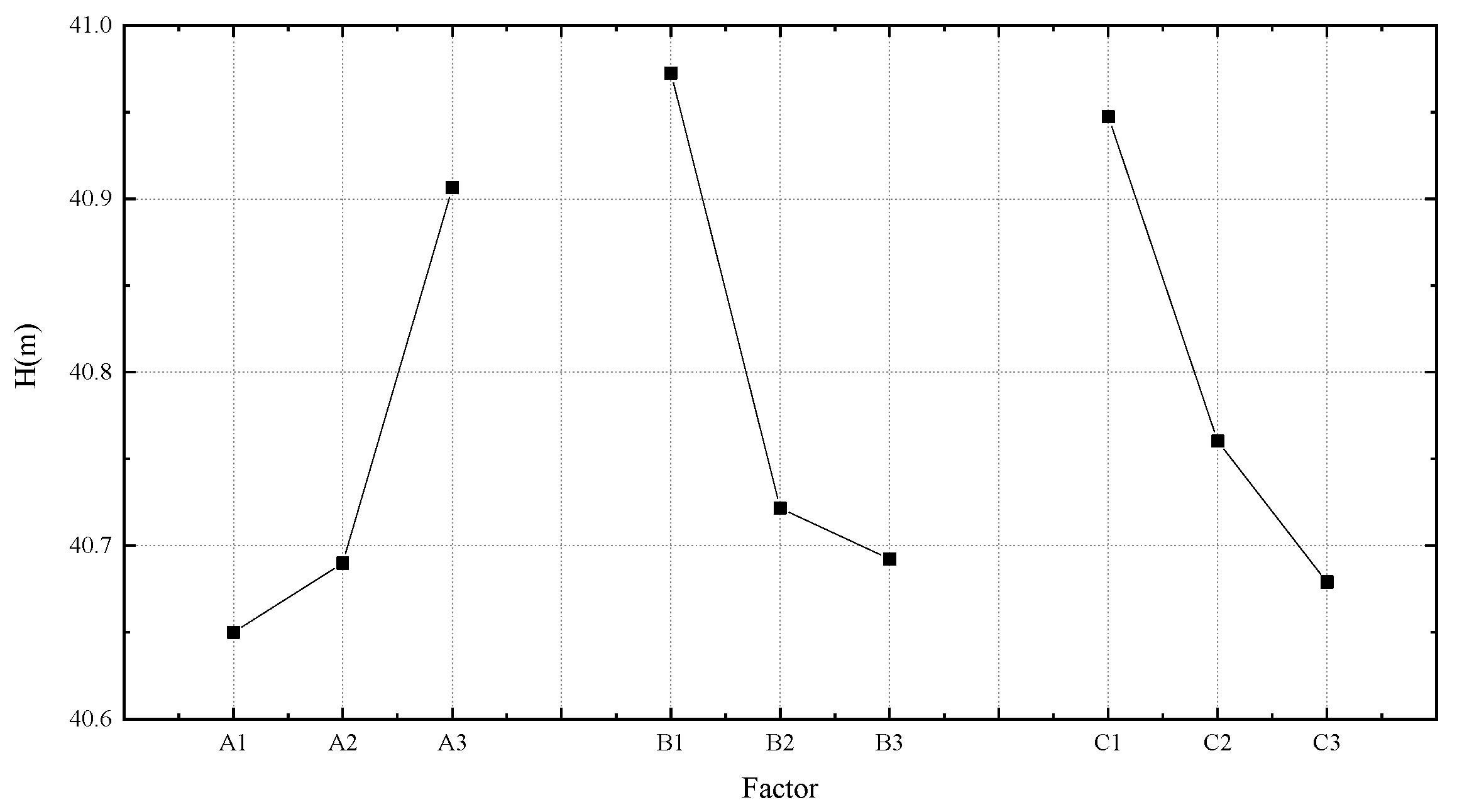
Based on the above analysis, the optimal solution for the pump head is A₃B₁C₁, with the following parameters: auxiliary blade quantity (Z) = 6, auxiliary blade inner diameter (R) = 44.4 mm, and auxiliary blade width (W) = 1. To simulate and calculate this data, a similar method to as mentioned previously was used for grid partitioning and computational modeling. After the calculations, under the operating condition of flow rate Q = 3.5 m³/h, the pump head was determined to be 41.39 m, the hydraulic efficiency was 37.98%, and the pump’s gland leakage rate was 1.36 kg/s.

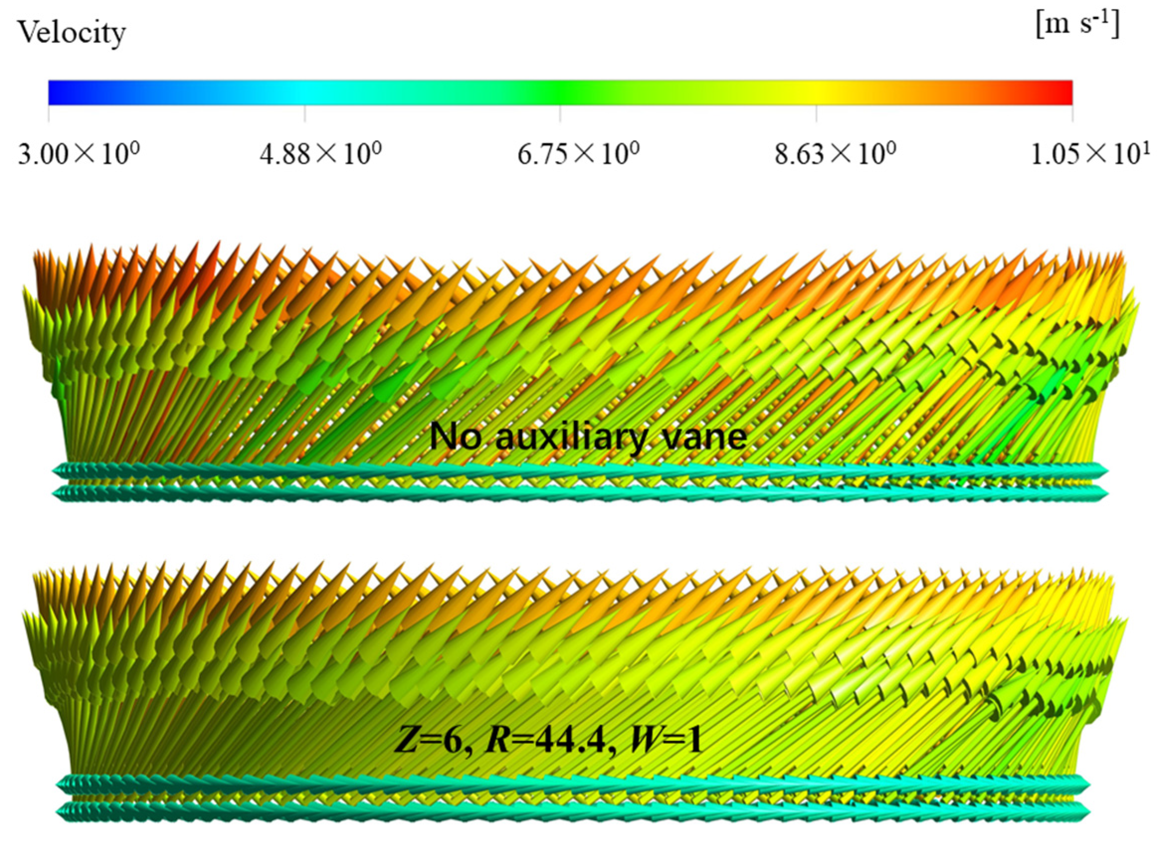
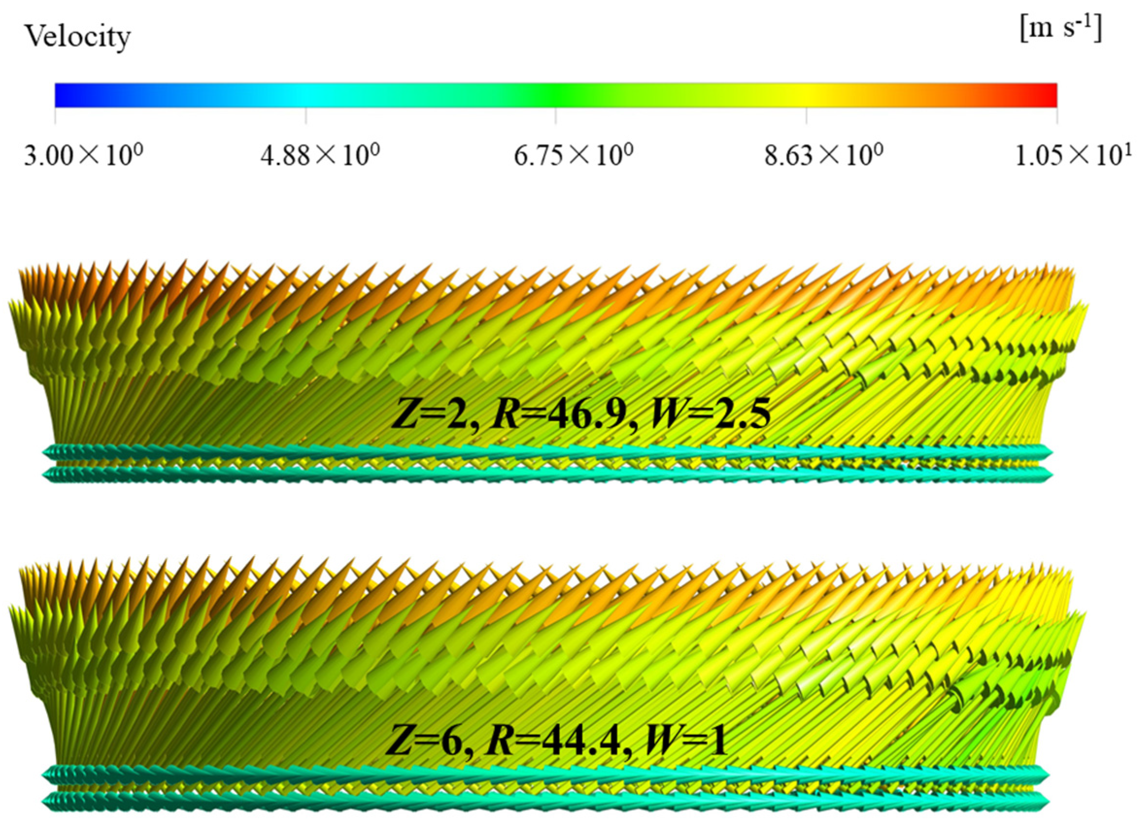
Figure 10 presents a comparative analysis of the flow field in the impeller front chamber for both the optimized and optimal solution schemes. Near the auxiliary blades, the fluid moves outward due to centrifugal force. Since the optimized solution has fewer and smaller auxiliary blades, there are significant areas without auxiliary blades. In these regions, the fluid velocity changes due to the guiding effect of the volute casing, and some of the fluid flows towards the center of the impeller. Subsequently, leakage flow occurs along the throat region, resulting in relatively significant volumetric losses. The optimal solution has six auxiliary blades, with larger radial and circumferential dimensions compared to the optimized solution. This allows it to generate centrifugal force on a larger volume of fluid. On the other hand, the optimized solution only has two auxiliary blades, and their radial dimensions are relatively smaller, resulting in a lower ability to prevent backflow compared to the optimal solution. The optimal solution exhibits lower leakage flow and relatively smaller volumetric losses, resulting in higher head for the same flow rate.

Figure 11 shows a comparison of the throat ring flow velocity vectors between the optimized scheme and the optimal solution scheme. It can be seen that the flow velocity color of the impeller in the optimized scheme is close to red, which is higher than the flow velocity of the impeller in the optimal solution scheme, resulting in a larger annular leakage volume per unit time. Intuitively, the impeller of the optimal solution scheme has a lower volumetric loss compared to the impeller of the optimized scheme. This is because, in the region between the volute casing and the impeller, where the leakage occurs, the optimal solution has a larger number of auxiliary blades, creating more high-pressure areas. This effectively reduces leakage at that location, resulting in lower velocities at the throat region.

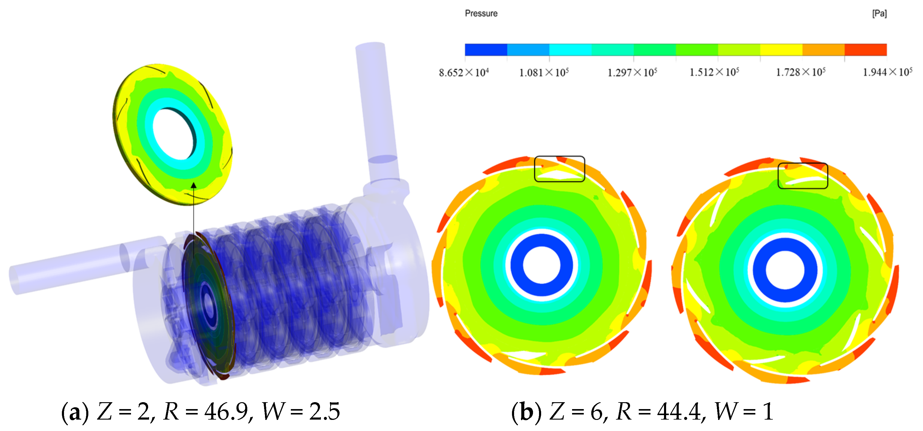
Figure 12 depicts a comparison of the pressure contour plots in the front chamber region between the optimized solution and the optimal solution. From the figure, it is evident that the presence of the auxiliary blades creates a high-pressure zone in the working surface. Therefore, in the vicinity of the high-pressure zone, the flow velocity decreases, which serves as a source of volute leakage. Consequently, the volumetric leakage rate per unit time decreases, resulting in a higher pump head. The optimized solution exhibits fewer high-pressure zones compared to the optimal solution, leading to a relatively higher volumetric leakage rate in the optimized solution. Additionally, the optimal solution features auxiliary blades with larger radial and circumferential dimensions, creating more high-pressure zones. This further emphasizes that the optimal solution can achieve smaller volumetric losses. Under the influence of the auxiliary blades, the water in the front chamber is subjected to centrifugal forces, causing it to flow outward and reducing the pressure in the front chamber. A low-pressure zone is formed near the center of the impeller, exhibiting a symmetrical distribution along the circumference. From the comparison plot, it can be observed that the low-pressure zone area in the optimal solution is larger than that in the optimized solution. The axial force in the rotor system primarily originates from the pressure difference between the front and rear sides of the impeller. Typically, the pressure on the outer side of the back cover plate is higher than that on the outer side of the front cover plate. Therefore, as the pressure on the outer side of the front cover plate decreases, the corresponding axial force increases. This indicates that the optimal solution generates a greater axial force when the impeller is in operation. Through calculations, it was determined that the pump bearings could withstand the increased axial force associated with the optimal solution.

The leakage through the throat ring is an important component of volumetric losses. The calculation formula for volumetric losses at the throat ring is given by Equation (11) [30].

$$Q_S=\mu A_{cl}\sqrt{2g\Delta H_{cl}}$$

(11)

where Qs is the leakage rate of the throat ring, A_cl represents the cross-sectional area of the throat ring, ΔH_cl is the difference in head on both sides of the throat ring, μ is the leakage coefficient, and g is gravitational acceleration.

Figure 13 presents a comparison of the total pressure on both sides of the throat ring between the optimized design and the optimal solution for the first-stage impeller. From the figure, it can be observed that the pressure difference across the throat ring is smaller for the optimal solution compared to the optimized design. According to Equation (11), when the difference in head between the two sides of the throat region is small, this corresponds to a lower leakage rate at the throat. This is because in the optimal solution, the difference in head between the two sides of the throat region is relatively small. It can be inferred that the leakage rate at the throat ring is lower for the optimal solution, resulting in relatively smaller volumetric losses. Under unchanged conditions, at the same flow rate, the optimal solution pump achieves a higher head.

Figure 14 shows a comparison of the turbulence kinetic energy contour maps of the water section in the pre-cavity of the impeller between the optimized scheme and the optimal solution scheme. As can be seen from the figure, the turbulence kinetic energy values in the inner region of the water body in the pre-cavity of the impeller of the optimized scheme are relatively low, with the values gradually increasing from the inside to the outside. From the lowest blue area outward, the turbulence kinetic energy exhibits irregularly alternating high and low changes. The turbulence kinetic energy is significantly increased on the inner side of the auxiliary blades, resulting in higher energy losses. Similarly, the inner side of the water body in the pre-cavity of the optimal solution scheme also has lower turbulence kinetic energy values, with the values gradually increasing from the inside to the outside. Near the auxiliary blades, the turbulence kinetic energy changes are relatively stable, resulting in less energy being lost. In the outermost region of the pre-cavity water body, the area where the dynamic water body of the auxiliary blades interacts with the static water body of the guide vanes causes a significant increase in turbulence kinetic energy, resulting in higher turbulent energy losses. By comparing the two schemes, it can be seen that the turbulence kinetic energy of the pre-cavity water body in the optimized scheme is significantly higher than that of the optimal solution scheme, indicating that the turbulent energy loss in the pre-cavity water body of the optimal solution is lower.

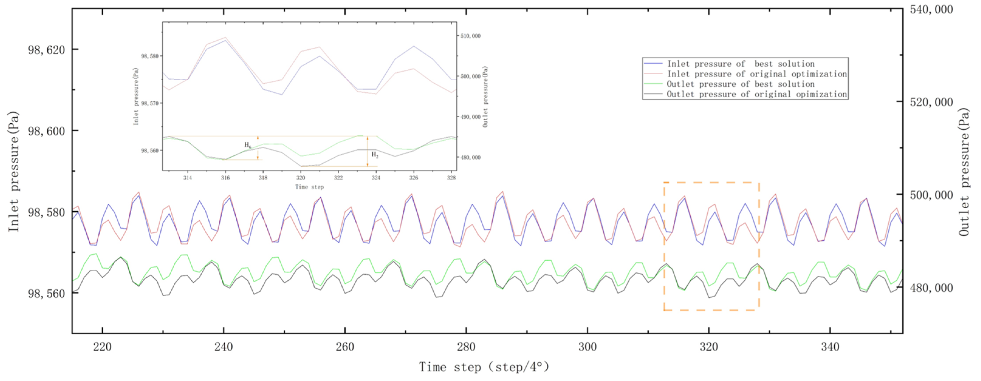
Based on the above simulation analysis, transient simulations were performed for both the optimized scheme and the optimal solution scheme. Pressure measurements were taken at the center of the pump inlet and outlet, with every 4° rotation of the impeller as a time step. The pressure fluctuations at each monitoring point were calculated at different rotation angles of the impeller. Figure 15 shows the trends of the pressure changes at the pump inlet and outlet pressure measurement points with the impeller rotation angle. Since the outlet pressure of the optimized scheme is lower than the outlet pressure of the optimal solution scheme, to facilitate comparison of the outlet pressure stability between the two schemes, the outlet pressure of the optimized scheme was increased by 10,000 Pa at each time step. Afterward, the pressure curves of the pump outlet for both schemes tended to be equal, allowing for a clearer comparison of the range of outlet pressure fluctuations.

As the total pressure inlet was used as the input, the pressures at the pump inlet can be seen to be similar in magnitude in the figure. At the pump outlet, the optimal solution had a relatively higher pressure value, corresponding to a higher head under the same flow conditions. The optimal solution scheme had a smaller range of outlet pressure fluctuations compared to the optimized scheme, with H₆ representing the pressure difference of the optimal solution and H₂ representing the pressure difference of the optimized scheme. This is because the optimal solution has six auxiliary blades, while the optimized solution only has two auxiliary blades. Additionally, each of the six blades in the optimal solution correspond to nine regular guide vanes, whereas the optimized solution only has two regular guide vanes. As a result, each blade in the optimal solution spends one-third of the time passing through the regular guide vanes, compared to in the optimized solution. This shorter duration of pressure change leads to a more stable pressure profile in the optimal solution. This indicates that the pump operation of the optimal solution scheme is more stable, with lower energy losses due to pressure fluctuations.

Table 9. Contour of Pressure in the Front Chamber at Different Rotating Angles of the Impeller.

Angle	20°	60°	100°	140°
Optimized scheme
Optimal solution scheme

shows the pressure contour maps of the pre-cavity water body at different impeller rotation angles. As can be seen from the figure, the high-pressure area on the working surface of the auxiliary blades in the optimized scheme is relatively smaller, and the outer circle of the pre-cavity water body is mostly a low-pressure area. When the dynamic water body in the low-pressure area rotates past the static water body of each guide vane, it comes into contact with the relatively higher pressure area of the guide vane water body. Near the contact area, there are significant pressure fluctuations. In the optimal solution scheme, the high-pressure area on the blade working surface in the outer circle of the pre-cavity water body is relatively larger, and the low-pressure area is relatively smaller. During rotation, the pressure difference between the low-pressure area and the high-pressure area of the guide vanes is relatively smaller, resulting in more stable pressure changes at the connected parts and smaller pressure impacts. The low-pressure area in the optimized scheme has two directions, while the low-pressure area in the optimal solution has six directions. During the impeller rotation process, the vibration frequency of the optimal solution is higher than that of the optimized scheme. By comparing the impeller at different rotation angles, the low-pressure area in the central region of the optimal solution is always larger than that of the optimized scheme, leading to a larger axial force in the optimal solution scheme. The area of the red high-pressure region inside the guide vanes of the optimal solution scheme is significantly larger than that of the optimized scheme. Both model pumps have the same flow velocity during the calculation process. Therefore, the scheme with higher pressure corresponded to a higher head, verifying the accuracy of the orthogonal test conclusion.

In summary, based on the analysis of flow velocity, pressure, total pressure, and turbulent kinetic energy, the head of the optimal solution scheme is higher than that of the optimized scheme. Figure 16 shows a comparison of the pump flow-head curves for the optimized scheme and the optimal solution scheme. As can be seen from the figure, the head of the optimal solution scheme is significantly higher than that of the optimized scheme. The head decreases as the flow rate increases. Within the entire flow range, the difference in head tended to be equal. Near the low flow rate, due to the relatively lower accuracy of the simulation, a larger difference was generated. From this figure, it can be inferred that the optimal solution better improved the head of the pump.

9. Optimal Solution Scheme Experimental Verification and Analysis

9.1. Test Preparation

Based on the above analysis, sample preparation was carried out and experimental verification was performed. As shown in Figure 17, a 1:1 print of the impeller front cover plate with auxiliary blades on A4 paper was made. The auxiliary blade portion was cut out and used as a template. The prepared template was attached to the outer side of the impeller front cover plate sample. The opening position of the auxiliary blades on the template was marked in black. After removing the template, the accurate position of the auxiliary blades was marked on the impeller front cover plate. Auxiliary blades made of 3D-printed PLA material were then attached to the corresponding black shadow positions using AB glue, creating an impeller with accurately positioned auxiliary blades. The impeller with auxiliary blades was assembled onto the multi-stage centrifugal pump in the correct order, and a pump performance test was conducted.

Figure 18 displays an image of the performance test for a multistage centrifugal pump. During the experimental process, pressure, flow rate, and rotational speed data were collected and input into the program for the calculation of the head and overall efficiency of the pump.

9.2. Experimental Results and Analysis

The experimental results showed that after adding auxiliary blades, the multi-stage centrifugal pump could operate normally, and the axial bearing capacity of the pump bearing met the usage requirements.

Figure 19 shows a comparison of the simulated calculation and experimental curves of the head and the efficiency for the optimal solution scheme pump. As can be seen from the figure, near the optimal operating point, the head deviation of the pump was 0.02%, proving the high accuracy of the simulation calculation. Near the high flow and low flow regions, the head deviation increased and the simulation accuracy gradually decreased. The efficiency shown in the figure is the hydraulic efficiency, which does not consider the energy loss in the process of the motor transferring energy to the pump, so the deviation from the experiment is relatively large. However, the simulated hydraulic efficiency and the experimental efficiency of the pump show the same trend and have the same optimal operating point. Comparing the experimental data of pumps with and without auxiliary blades, the head and efficiency of the pump were improved after adding auxiliary blades. As a further explanation, the combination of orthogonal experimental design and grey relational analysis methods could be more accurately used for multi-stage centrifugal pump impeller structure optimization. By using these methods together, it was possible to efficiently evaluate the performance of various design alternatives and identify the optimal impeller structure for multi-stage centrifugal pumps.

10. Conclusions

The structure of auxiliary blades has different impacts on pump performance. In this study, a combination of orthogonal experimental design and grey relational analysis methods was applied. Through the analysis of flow velocity, pressure, total pressure, and turbulent kinetic energy, the following conclusions were drawn:

• Increasing the number of auxiliary blades could improve the pump’s head. In the optimized solution, the auxiliary blade structure was defined as Z = 2, R = 46.9 mm, and W = 2.5. Near the optimal operating point, the optimized solution achieved a 6% increase in head compared to the original solution. This increase was more pronounced at high flow rates, where the pump’s head was elevated by approximately 23%. However, the increase in head was not significant at low flow rates.
• Based on the factors of the blade number Z, radial dimension R, and width W, the method combining simulation calculation and orthogonal experiment was feasible for the design optimization of auxiliary blades for multi-stage centrifugal pumps. This method could accurately infer the optimal solution of the head corresponding to various parameters of the multi-stage centrifugal pump auxiliary blades.
• The combination of orthogonal experiment and grey relational analysis methods was used to perform dimensionless processing on the reference series and comparison series, and to more accurately infer the primary and secondary factors affecting the head. The head of the multi-stage centrifugal pump was improved by adjusting the primary and secondary factors, to better meet the usage requirements. The primary and secondary factors affecting the head of the multi-stage centrifugal pump were the radial length R, width W, and number Z of the auxiliary blades.
• Comparing the optimal solution scheme with the optimized scheme, it was found that, under the same flow rate conditions, the optimal solution scheme had a smaller outlet pressure fluctuation range, more stable operation, and lower energy loss due to pressure fluctuation than the optimized scheme.

References

1. Chen, Q.R.; Shu, T.; Liu, M.; Cui, M.Y. Armature optimization design based on orthogonal test. J. Phys. Conf. Ser. 2019, 1284, 012018. [Google Scholar] [CrossRef] [Green Version]
2. Chang, H.; Shi, W.; Li, W.; Wang, C.; Zhou, L.; Liu, J.; Yang, Y.; Ramesh, K.A. Experimental Optimization of Jet Self-Priming Centrifugal Based on Orthogonal Design and Grey-Correlational Method. J. Therm. Sci. 2020, 29, 241–250. [Google Scholar] [CrossRef]
3. Yang, Y.; Zhou, L.; Zhou, H.; Lv, W.; Wang, J.; Shi, W.; He, Z. Optimal Design of Slit Impeller for Low Specific Speed Centrifugal Pump Based on Orthogonal Test. J. Mar. Sci. Eng. 2021, 9, 121. [Google Scholar] [CrossRef]
4. Quan, H.; Guo, Y.; Li, R.; Su, Q.; Chai, Y. Optimization design and experimental study of vortex pump based on orthogonal test. Sci. Prog. 2020, 103, 003685041988188. [Google Scholar] [CrossRef] [PubMed] [Green Version]
5. Wang, Y.; Ding, Z. Optimization design of hump phenomenon of low specific speed centrifugal pump based on CFD and orthogonal test. Sci. Rep. 2022, 12, 12121. [Google Scholar]
6. Pei, J.; Yin, T.; Yuan, S.; Wang, W.; Wang, J. Cavitation Optimization for a Centrifugal Pump Impeller by Using Orthogonal Design of Experiment. Chin. J. Mech. Eng. 2017, 30, 109. [Google Scholar] [CrossRef]
7. Wang, C. Research on Energy Loss and Self-Priming Mechanism of Low-Specific-Speed Multi-Stage Self-Priming Sprinkler Pump; Jiangsu University: Zhenjiang, China, 2016. [Google Scholar]
8. Zhang, Y.; Xu, Y.; Zheng, Y.; Fernandez-Rodriguez, E.; Sun, A.; Yang, C.; Wangm, J. Multiobjective Optimization Design and Experimental Investigation on the Axial Flow Pump with Orthogonal Test Approach. Complexity 2019, 2019, 1467565. [Google Scholar] [CrossRef] [Green Version]
9. Yun, L.; Rongsheng, Z.; Wang, D.-Z.; Junlian, Y.; Tianbin, L. Numerical and experimental investigation on the diffuser optimization of a reactor coolant pump with orthogonal test approach. J. Mech. Sci. Technol. 2016, 30, 4941–4948. [Google Scholar] [CrossRef]
10. Liu, M.; Tan, L.; Cao, S. Design Method of Controllable Blade Angle and Orthogonal Optimization of Pressure Rise for a Multiphase Pump. Energies 2018, 11, 1048. [Google Scholar] [CrossRef] [Green Version]
11. Shi, G.; Li, H.; Liu, X.; Liu, Z.; Wang, B. Transport Performance Improvement of a Multiphase Pump for Gas–Liquid Mixture Based on the Orthogonal Test Method. Processes 2021, 9, 1402. [Google Scholar] [CrossRef]
12. Sun, Z.; Wang, X.; Shi, L.; Tang, F. Hydraulic performance and flow patterns of axial-flow pumps with axial stacking of different airfoil series. J. Drain. Irrig. Mach. Eng. 2022, 40, 217–222. [Google Scholar]
13. Liu, H.; Du, X.; Wu, X.; Tan, M. Numerical simulation on gas-phase characteristics of gas-liquid two-phase flow in pump. J. Drain. Irrig. Mach. Eng. 2022, 40, 238–243. [Google Scholar]
14. Khaled, A.; Bashar Ar Mosab, A.; Ahmed, M. Evaluation of the Erosion Characteristics for a Marine Pump Using 3D RANS Simulations. Appl. Sci. 2021, 11, 7364. [Google Scholar]
15. Kong, D.; Pan, Z.; Yang, B. Characteristics of gas-liquid two-phase flow in self-priming pump. J. Drain. Irrig. Mach. Eng. 2022, 40, 15–21. [Google Scholar]
16. Stel, H.; Ofuchi, E.M.; Chiva, S.; Morales, R.E.M. Numerical simulation of gas-liquid flows in a centrifugal rotor. Chem. Eng. Sci. 2020, 221, 115692. [Google Scholar] [CrossRef]
17. Ikhlaq, M.; Al-Abdeli, Y.M.; Khiadani, M. Nozzle exit conditions and the heat transfer in non-swirling and weakly swirling turbulent impinging jets. Heat Mass Transf. 2020, 56, 269–290. [Google Scholar] [CrossRef]
18. Huang, J.; Zheng, Y.; Kan, K.; Xu, Z.; Huang, C.; Zhou, G.; Du, Y. Hydraulic characteristics of reverse power generation of axial-flow pump. J. Drain. Irrig. Mach. Eng. 2022, 40, 230–237. [Google Scholar]
19. Li, W.; Li, E.; Ji, L.; Zhou, L.; Shi, W.; Zhu, Y. Mechanism and propagation characteristics of rotating stall in a mixed-flow pump. Renew. Energy 2020, 153, 74–92. [Google Scholar] [CrossRef]
20. Li, W.; Ji, L.; Li, E.; Shi, W.; Agarwal, R.; Zhou, L. Numerical investigation of energy loss mechanism of mixed-flow pump under stall condition. Renew. Energy 2021, 167, 740–760. [Google Scholar] [CrossRef]
21. Li, W.; Ji, L.; Li, E.; Zhou, L.; Agarwal, R.K. Effect of tip clearance on rotating stall in a mixed-flow pump. ASME J. Turbomach. 2021, 143, 091013. [Google Scholar] [CrossRef]
22. Wei, L.; Huang, Y.; Ji, L.; Ma, L.; Agarwal, R.K.; Awais, M. Prediction model for energy conversion characteristics during transient processes in a mixed-flow pump. Energy 2023, 271, 127082. [Google Scholar]
23. Ji, L.; Li, W.; Shi, W.; Chang, H.; Yang, Z. Energy Characteristics of Mixed-Flow Pump under Different Tip Clearances Based on Entropy Production Analysis. Energy 2020, 199, 117447. [Google Scholar] [CrossRef]
24. Ji, L.; Li, W.; Shi, W.; Tian, F.; Agarwal, R. Effect of Blade Thickness on Rotating Stall of Mixed-Flow Pump Using Entropy Generation Analysis. Energy 2021, 236, 121381. [Google Scholar] [CrossRef]
25. Ji, L.; Li, W.; Shi, W.; Tian, F.; Agarwal, R. Diagnosis of internal energy characteristics of mixed-flow pump within stall region based on entropy production analysis model. Int. Commun. Heat Mass Transf. 2020, 117, 104784. [Google Scholar] [CrossRef]
26. Ji, L.; He, S.; Li, W.; Shi, W.; Li, S.; Li, H.; Agarwal, R. Exploration of Blade Thickness in Suppressing Rotating Stall of Mixed Flow Pump. Arab. J. Sci. Eng. 2023, 48, 8227–8251. [Google Scholar] [CrossRef]
27. Ji, L.; He, S.; Li, Y.; Wei, L.; Shi, W.; Li, S.; Yang, Y.; Yang, Y.; Gao, Y.; Agarwal, R.K. Investigation of energy loss mechanism of shroud region in A mixed-flow pump under stall conditions. Proc. Inst. Mech. Eng. Part A J. Power Energy 2023. [Google Scholar] [CrossRef]
28. Li, W.; Liu, M.; Ji, L.; Li, S.; Song, R.; Wang, C.; Cao, W.; Agarwal, R.K. Study on the trajectory of tip leakage vortex and energy characteristics of mixed-flow pump under cavitation conditions. Ocean Eng. 2023, 267, 113225. [Google Scholar] [CrossRef]
29. Zhou, L.; Shi, W.; Lu, W.; Xu, R.; Wang, C. Orthogonal test and optimization design of submersible pump guide vanes. J. Drain. Irrig. Mach. Eng. 2011, 29, 312–315. [Google Scholar]
30. Fu, J.; Li, H.; Fan, D.; Shen, W.; Liu, X. Modeling and Efficiency Prediction of Aeroengine Centrifugal Pump Integrated Loss Model Based on One-Dimensional Flow. J. Northwestern Polytech. Univ. 2018, 36, 807–815. [Google Scholar] [CrossRef]
Figure 1. Multi-stage centrifugal pump. 1. Inlet cover 2. Guide vane 3. Impeller 4. Runner guide vane 5. Discharge chamber 6. Cylinder body.
Water 15 02465 g001
Figure 2. Impeller with auxiliary blade. (a) Without blade; (b) With blade, Z = 2, R = 46.98, W = 2.5.
Water 15 02465 g002
Figure 3. Five stage centrifugal pump and water model.
Water 15 02465 g003
Figure 4. Water body mesh.
Water 15 02465 g004
Figure 5. Comparison diagram of the simulation and test.
Water 15 02465 g005
Figure 6. Velocity vector diagrams for schemes with and without auxiliary blades.
Water 15 02465 g006
Figure 7. Comparison of throat ring velocity vector diagrams for the schemes with and without auxiliary blades.
Water 15 02465 g007
Figure 8. Impeller structure illustration.
Water 15 02465 g008
Figure 9. Trend chart of head-factors.
Water 15 02465 g009
Figure 10. Comparison of impeller front chamber flow vector between the optimized and optimal solution schemes.
Water 15 02465 g010
Figure 11. Comparison of the throat ring flow vector between the optimized and optimal solution schemes.
Water 15 02465 g011
Figure 12. Comparison of the front chamber pressure contour between the optimized and optimal solution scheme.
Water 15 02465 g012
Figure 13. Comparison of the total pressure contour between the optimized and optimal solution schemes.
Water 15 02465 g013
Figure 14. Comparison of the turbulence kinetic energy contours between the optimized and optimal solution schemes.
Water 15 02465 g014
Figure 15. Comparison of the inlet and outlet pressure between the optimized and optimal solution schemes.
Water 15 02465 g015
Figure 16. Simulated heads between the optimized and optimal solution schemes.
Water 15 02465 g016
Figure 17. Prototype of the impeller.
Water 15 02465 g017
Figure 18. Performance test.
Water 15 02465 g018
Figure 19. Comparison between the simulation and experiment of the optimal solution scheme.
Water 15 02465 g019