Runoff Prediction Based on Dynamic Spatiotemporal Graph Neural Network

Abstract

Runoff prediction plays an important role in the construction of intelligent hydraulic engineering. Most of the existing deep learning runoff prediction models use recurrent neural networks for single-step prediction of a single time series, which mainly model the temporal features and ignore the river convergence process within a watershed. In order to improve the accuracy of runoff prediction, a dynamic spatiotemporal graph neural network model (DSTGNN) is proposed considering the interaction of hydrological stations. The sequences are first input to the spatiotemporal block to extract spatiotemporal features. The temporal features are captured by the long short-term memory network (LSTM) with the self-attention mechanism. Then, the upstream and downstream distance matrices are constructed based on the river network topology in the basin, the dynamic matrix is constructed based on the runoff sequence, and the spatial dependence is captured by combining the above two matrices through the diffusion process. After that, the residual sequences are input to the next layer by the decoupling block, and, finally, the prediction results are output after multi-layer stacking. Experiments are conducted on the historical runoff dataset in the Upper Delaware River Basin, and the MAE, MSE, MAPE, and NSE were the best compared with the baseline model for forecasting periods of 3 h, 6 h, and 9 h. The experimental results show that DSTGNN can better capture the spatiotemporal characteristics and has higher prediction accuracy.

1. Introduction

Accurate and reliable prediction of river basin inner diameter flow is of great significance for water resource management, flood control and disaster reduction, and hydropower generation [1]. Runoff is influenced by natural and human factors and has nonlinear, nonstationary, and complex time-varying characteristics [2]. Accurate prediction of it is currently a hot research topic. At present, the means of collecting water conservancy information are changing rapidly, and various advanced observation equipment has been put into use. Water conservancy information has reached the level of big data. Analyzing and applying relevant water conservancy information based on the latest achievements in the field of information is a major goal of the development of intelligent hydraulic engineering. Deep learning can directly establish end-to-end connections and better capture implicit relationships between inputs and outputs [3]. Deep learning technology is widely used in the field of water resources due to its nonlinear mapping ability and high robustness [4]. It can directly extract implicit information from historical hydrological data for prediction.

In order to improve the prediction performance of hydrological time series deep learning models, researchers mainly focus on the following three aspects:

• Using new technologies, models, and methods emerging from deep learning. Lv et al. [5] extracted hydrological features such as rainfall, reservoir water level, and flow, and used LSTM to model the rainfall runoff process. The results showed that LSTM was capable of long-term and short-term hydrological forecasting. Tao et al. [6] proposed a multi-scale LSTM model with the self-attention mechanism (MLSTM-AM) for predicting monthly precipitation at stations in the Yangtze River Basin. Wang et al. [7] used attention mechanisms for hydrological sequence features for runoff prediction, and experimental results showed that the attention module improved learning and generalization capabilities. Xie et al. [8] used an integrated learning model of 1D CNN and 2D CNN to improve the daily runoff prediction accuracy.
• Using different optimization algorithms to improve the performance of existing models. The hyperparameter has a significant impact on the performance of the depth model. Through the optimization algorithm, the correct combination of hyperparameter values can be found, and the maximum performance can be achieved in a reasonable time, which can improve the prediction accuracy and robustness of the model. Zhao et al. [9] designed a hybrid model IGWO-GRU which combed GRU and improved grey wolf optimizer to predict the monthly runoff at the Fenhe reservoir station. Khadr et al. [10] constructed an optimization simulation framework based on implicit stochastic optimization, genetic algorithm, and recurrent neural network to predict reservoir inflow and water use, and guide reservoir scheduling. Qiu et al. [11] used the particle swarm optimization algorithm and back propagation neural network to predict river water temperature using input variables such as temperature, flow, and date.
• Using signal decomposition or denoising techniques to preprocess data. Data preprocessing mainly involves using various signal decomposition and denoising techniques to stabilize the runoff series, decompose it into simpler or meaningful components, and then model them separately. Bai et al. [12] proposed the MDFL method for predicting the daily inflow of reservoirs. The method uses the empirical mode decomposition and Fourier transform to extract trend, periodic, and random features, and then trains them with three deep belief networks. Finally, the prediction results are reconstructed. Li et al. [13] developed a hybrid model of adaptive variational mode decomposition and bidirectional long short-term memory (Bi-LSTM) based on energy entropy to predict daily inflow. Huang et al. [14] presented a prediction model combining the ensemble empirical mode decomposition and LSTM to predict the runoff of the irrigated paddy areas in Southern China.

The above models mainly focus on the runoff sequence of a single hydrological station as the research object, limited to the temporal characteristics of the station, and insufficient mining of spatiotemporal features within the basin, ignoring rich geographic information, mainly the spatial distribution relationship of the station and the convergence process of water flow.

Graph neural networks [15] can extract information from graph structures in non-Euclidean spaces and are widely used in social networks [16], recommender systems [17], protein and drug action [18], anomaly detection [19], etc., and have shown good performance. Graph neural networks are applied to extract spatial features in runoff prediction. Sun et al. [20] proposed a multi-stage, physically driven graph neural network method, which trains GNN models with performance similar to high-resolution moderate river network models, for river network learning and flow prediction at watershed scale. Liu et al. [21] considered the spatial connectivity of different stations in actual watersheds and constructed a watershed network based on graph data structure. At the same time, they combined variational reasoning with edge condition convolutional networks and proposed the variational Bayesian edge condition graph convolutional model (VBEGC) for daily flow prediction. Xiang et al. [22] proposed a fully distributed rainfall runoff deep learning model based on physical processes, which applied the LSTM time series model to calculate the runoff yield on each grid unit. The GNN then aggregated the output of each grid unit to calculate the final runoff at the outlet of the watershed.

In summary, the existing runoff prediction model based on graph neural networks only uses the features of covariates extracted by graph neural networks to predict runoff sequences at a single station, not directly modeling the runoff sequences at all stations and not sufficiently mining the spatial and temporal features of the whole watershed. To solve this problem, this article proposes a dynamic spatiotemporal graph neural network model (DSTGNN) for runoff prediction based on its temporal and spatial characteristics. The model abstracts hydrological stations as nodes, natural river connections between stations as edges, and hydrological station runoff within the region as graph signal data. The main work of this article is as follows:

(1)

A runoff prediction model has been proposed, which decomposes runoff formation into the runoff production process and river network convergence process, integrating physical processes on the basis of data-driven models;

(2)

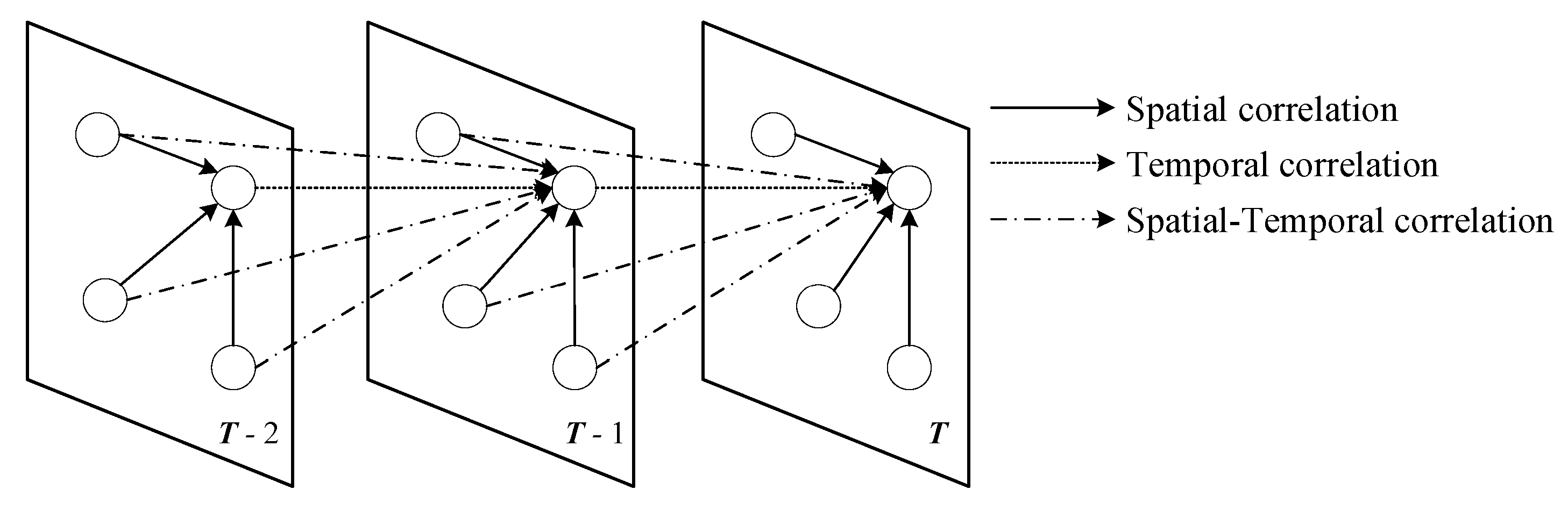
Under the above framework, the LSTM model with the self-attention mechanism is used to enhance the ability to capture the time-series characteristics of runoff. Construct a directed graph of upstream stations pointing towards downstream stations based on the geographic spatial structure of a tree-like river network, and capture the spatial relationships of stations within the watershed through a graph neural network;

(3)

This model is applicable to the entire watershed, mining the runoff characteristics of the entire watershed, and providing multi-step runoff prediction for all stations within the watershed in advance.

The rest of the paper is organized as follows. Section 2 provides a formal definition of multisite prediction. Section 3 describes the model proposed in this paper. Section 4 contains experimental details and an analysis of the results. Section 5 describes the conclusion and outlook of our work.

2. Multiple Stations Runoff Prediction

The goal of this article is to predict the future runoff of multiple stations based on historical data by constructing topological relationships on the river network. Represent the site network as a weighted directed graph G = (V, E, W), where V is the set of stations, |V| = N; E is the edge of the graph, representing the upstream and downstream relationships; $\mathit{W}\in R^{N\times N}$ is the distance adjacency matrix. Represent the observed runoff data on graph G as features $\mathit{X}\in R^{N\times P}$, where P is the number of features. X(t) represents the observed node characteristics at time t. The prediction problem aims to learn a function h (·) to predict the runoff of all stations in the future time slot based on historical observation data:

$$[{\mathit{X}}^{(t-H+1)},\cdot \cdot \cdot ,{\mathit{X}}^{(t)};G]\stackrel{h(·)}{\to }[{\mathit{X}}^{(t+1)},\cdot \cdot \cdot ,{\mathit{X}}^{(t+F)}].$$

(1)

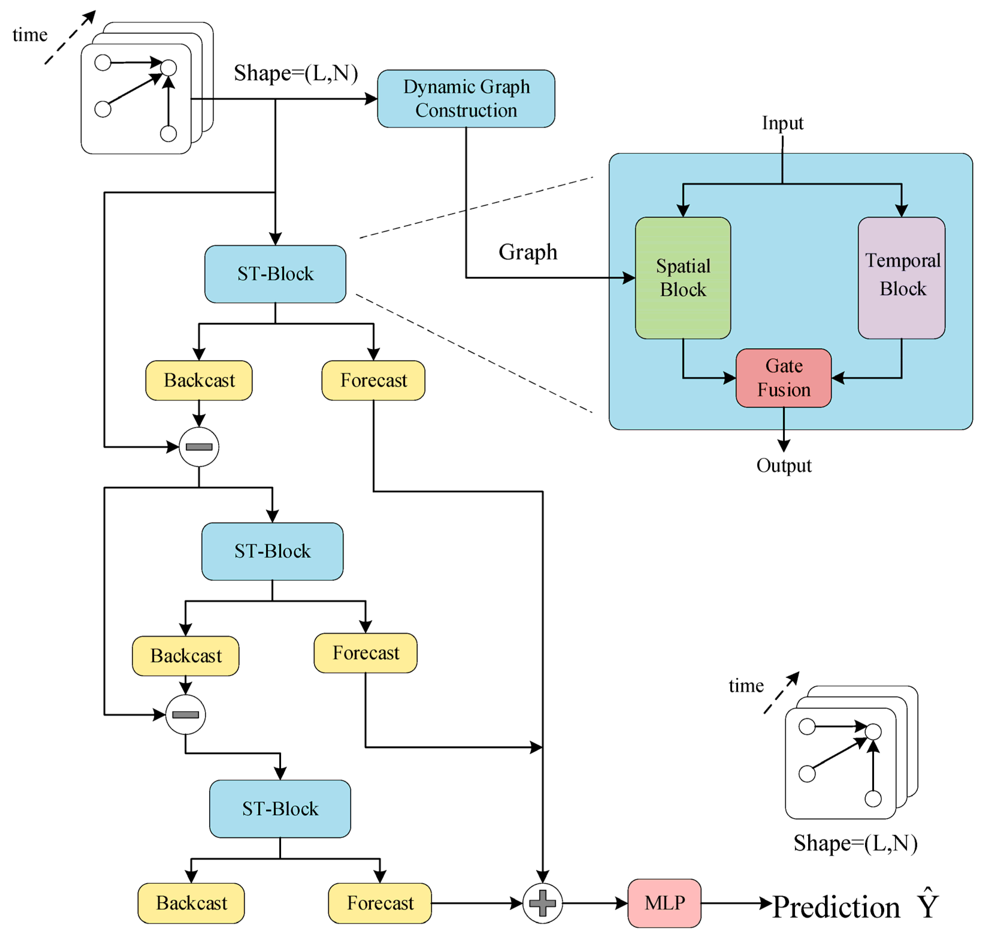
3. Dynamic Graph Neural Network Prediction Model

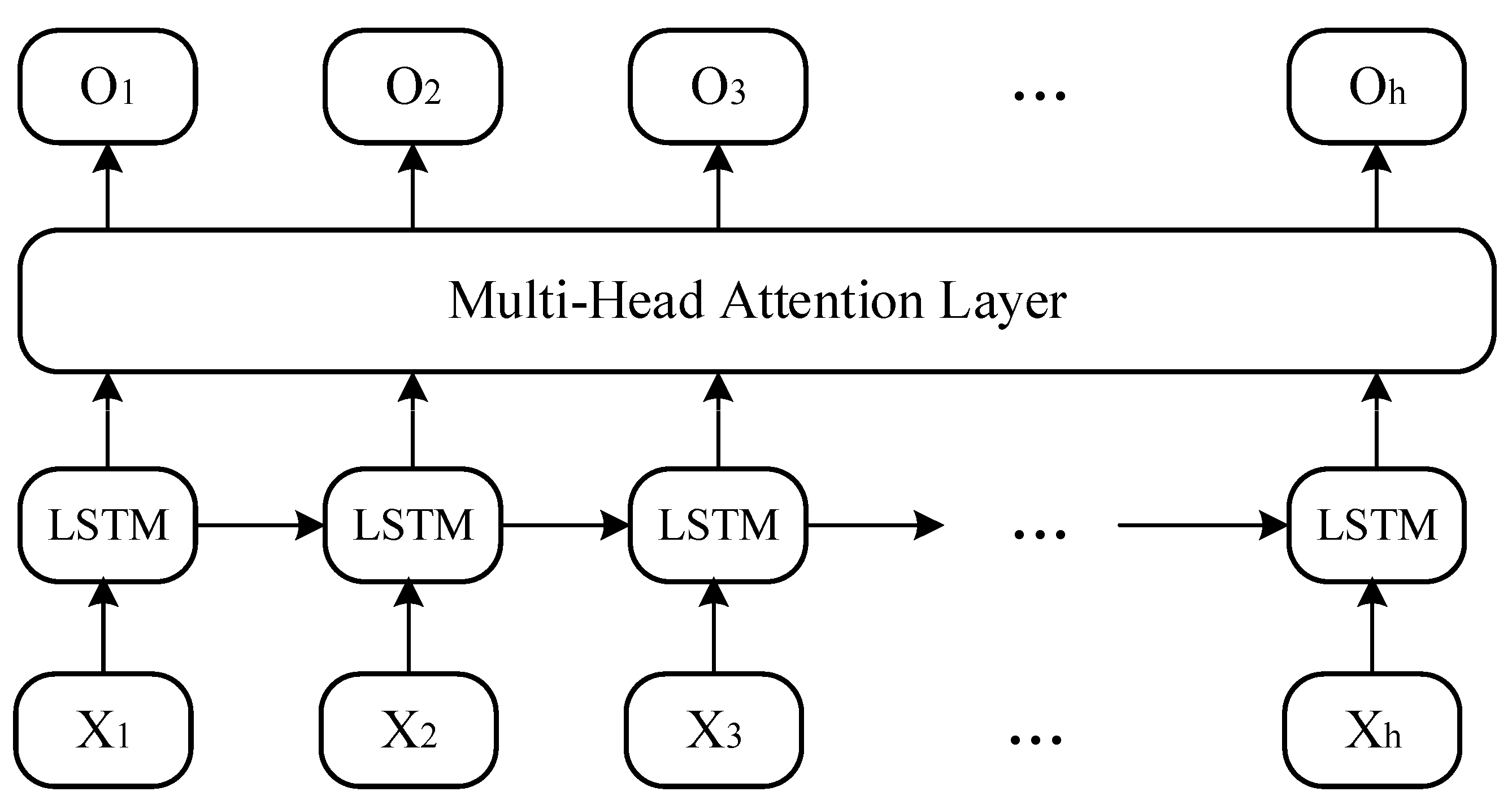
As shown in Figure 1, multi-site runoff prediction is a complex spatiotemporal prediction problem, where the current runoff at the site is both related to historical runoff and influenced by surrounding sites. Therefore, this article proposes a dynamic spatiotemporal graph neural network model (DSTGNN) for runoff prediction based on its characteristics.

The model as Figure 2, is divided into a spatiotemporal feature extraction block, a residual block, and a prediction output block. Firstly, the runoff sequence $\mathit{X}\in R^{L\times N\times 1}$ is mapped to high-dimensional through a linear layer, and then inputted into the spatiotemporal block extract spatiotemporal features. Then, the predicted hidden state and the residual value input to the next layer are obtained through the prediction block and residual decomposition, respectively. Finally, based on the hidden states obtained from each layer, the predicted values are output through two fully connected layers.

3.1. Temporal Block

The temporal block as Figure 3 is used to capture the time dependence of a single site runoff sequence, focusing on events in nearby control watersheds. This module captures the overall situation of the watershed by capturing the changes in flow at each station over time and synthesizing them all together.

The LSTM [23] model can learn close-range dependency information and alleviate the long-term dependency problem by introducing gating mechanisms and adding unit states. However, as the distance increases, the model’s ability to capture long-range dependencies gradually decreases. The self-attention [24] mechanism, on the other hand, is better at handling long-term dependencies [25], and can capture important combinations from input features, highlighting key local information. Therefore, this article utilizes LSTM and multi-head self-attention to capture time dependence and learn important features in the input.

LSTM is a special form of recurrent neural network model proposed to solve the problem of gradient vanishing and exploding during long sequence training. The LSTM unit consists of three gate structures: the forgetting gate ${\mathit{f}}_t$, the input gate ${\mathit{i}}_t$, and the output gate ${\mathit{o}}_t$. Given the current input ${\mathit{x}}_t$, previous output ${\mathit{h}}_{t-1}$, and unit state ${\mathit{C}}_{t-1}$, each gate is calculated as follows:

$${\mathit{f}}_t=\sigma ({\mathit{W}}_f\cdot [{\mathit{h}}_{t-1},{\mathit{x}}_t]+{\mathit{b}}_f)$$

(2)

$${\mathit{i}}_t=\sigma ({\mathit{W}}_i\cdot [{\mathit{h}}_{t-1},{\mathit{x}}_t]+{\mathit{b}}_i)$$

(3)

$${\hat{\mathit{C}}}_t=\phi ({\mathit{W}}_c\cdot [{\mathit{h}}_{t-1},{\mathit{x}}_t]+{\mathit{b}}_c)$$

(4)

$${\mathit{C}}_t={\mathit{f}}_t\cdot {\mathit{C}}_{t-1}+{\mathit{i}}_t\cdot {\hat{\mathit{C}}}_t$$

(5)

$${\mathit{o}}_t=\sigma ({\mathit{W}}_o\cdot [{\mathit{h}}_{t-1},{\mathit{x}}_t]+{\mathit{b}}_o)$$

(6)

$${\mathit{h}}_t={\mathit{o}}_t\cdot \phi ({\mathit{C}}_t)$$

(7)

where ${\mathit{W}}_f,{\mathit{W}}_i,{\mathit{W}}_c,{\mathit{W}}_o$ are, respectively, the weight matrix of each gate, ${\mathit{b}}_f,{\mathit{b}}_i,{\mathit{b}}_c,{\mathit{b}}_o$ represent the corresponding offset term, $\sigma$ and $\phi$ represent sigmoid and tanh activation functions, and ${\hat{\mathit{C}}}_t$ represents the status of candidate units. Through multi-step iteration of LSTM, the relevant information is sequentially transmitted backward, capturing short-term dependencies of temporal relationships. Long-term dependence is captured through the multi-head self-attention mechanism.

The original time series is processed through the LSTM layer to obtain the output $\mathit{\chi }\in R^{T_h\times N\times d}$, which is then linearly transformed to obtain the query, key, and value:

$$\mathit{Q}=\mathit{\chi }{\mathit{W}}^q,\mathit{K}=\mathit{\chi }{\mathit{W}}^k,\mathit{V}=\mathit{\chi }{\mathit{W}}^v$$

(8)

where ${\mathit{W}}^q,{\mathit{W}}^k,{\mathit{W}}^v\in R^{NC\times d}$; then, calculate the similarity between Q and each K, normalize it to obtain the self-attention coefficient, and dot product it with the corresponding key-value V to obtain the final attention value:

$$Atten(\mathit{Q},\mathit{K},\mathit{V})=\mathrm{softmax}(\frac{\mathit{Q}{\mathit{K}}^{\mathrm{T}}}{\sqrt{d}})\mathit{V}.$$

(9)

Multi-head attention refers to the pooling of attention by querying through parallel sets of independent linear projection transformations, keys, and values. Finally, concatenate each output together to produce the final output. The expression is as follows:

$${\mathit{h}}_i=Attention(\mathit{Q}{\mathit{W}}_i^q,\mathit{K}{\mathit{W}}_i^k,\mathit{V}{\mathit{W}}_i^v)$$

(10)

$$\mathit{O}=MultiH(\mathit{Q},\mathit{K},\mathit{V})=Concat({\mathit{h}}_1,\cdots ,{\mathit{h}}_n){\mathit{W}}_O$$

(11)

where O is the multi-head attention output matrix, n is the number of attention heads, and h_i represents the result of each attention operation.

The time feature ${\mathit{H}}_k^{\mathrm{tem}}$ obtained from the k-th input sequence through the temporal block is output to subsequent modules.

3.2. Spatial Block

The temporal block focuses on the temporal connections of the same node, whereas the spatial block focuses on capturing spatial dependencies between different nodes. From a spatial perspective, consider the flow of water from upstream stations to the next station, and integrate the water exchange between all stations to explore basin characteristics. This module constructs a corresponding matrix to express spatiotemporal dependence based on the unidirectional fluidity of water flow, where the flow value of downstream nodes depends on upstream nodes.

3.2.1. Distance Weight Matrix

This article abstracts the upstream and downstream relationships of hydrological stations into a directed graph G = (V, E), where G represents the topological structure of the spatial distribution of stations; V represents each node; E represents the length of the river $d_{i,j}$ between two stations. The weighted adjacency matrix $\mathit{A}\in R^{N\times N}$ is defined as follows:

$$\mathit{A}=\left[\begin{array}{cccc}0& a_{1,2}& \cdots & a_{1,N}\\ a_{2,1}& 0& \cdots & a_{2,N}\\ ⋮& ⋮& 0& ⋮\\ a_{N,1}& a_{N,2}& \cdots & 0\end{array}\right]$$

(12)

where N represents the number of sites; a_i,j = d_i,j when node j is a direct downstream node of node i, otherwise a_i,j = ∞.

The multiple stations in the Upper Delaware River Basin form a tree structure, whereas the adjacency matrix represents only spatial upstream–downstream relationships, focusing on first-order connectivity and neglecting indirect connections between nodes. According to the first law of geography, it can also be seen from Figure 4 that the closer the stations are to each other, the more similar their flow sequences are. In this paper, the corresponding weight matrix is constructed according to the distance between stations and the unidirectional mobility of water flow according to Algorithm 1. The distance weights are calculated as follows:

$${\mathit{D}}_{ij}=\exp (-\frac{dist{(v_i,v_j)}^2}{{\sigma }^2})$$

(13)

where dist (vi, vj) represents the shortest distance from vi to vj and $\sigma$ is the standard deviation of the distance.

Algorithm 1: Distance weight matrix D.

Input: Adjacency matrix A

Output: Distance weight matrix D

1 Initialize matrix D = A

2 for k = 1 to N do

3  for i = 1 to N do

4    for j = 1 to N do

5      D[i][j] = min(D[i][j], D[i][k] + D[k][j])

// Calculate the shortest distance according to Floyd algorithm

6 end for

7 for i = 1 to N do

8  for j = 1 to N do

9    Calculate D[i][j], as shown in Equation (13)

10 end for

11 Return D

3.2.2. Dynamic Matrix

For the runoff sequences X ∈ Rⁿ and Y ∈ Rⁿ of two stations, use the Pearson correlation coefficient to measure the similarity between the two:

$${\rho }_{X,Y}=\frac{cov(\mathit{X},\mathit{Y})}{{\sigma }_X{\sigma }_Y}=\frac{{\displaystyle \sum (\mathit{X}-\overline{\mathit{X}})(\mathit{Y}-\overline{\mathit{Y}})}}{\sqrt{{\displaystyle \sum _{i=1}^n{({\mathit{X}}_i-\overline{\mathit{X}})}^2}}\sqrt{{\displaystyle \sum _{i=1}^n{({\mathit{Y}}_i-\overline{\mathit{Y}})}^2}}}$$

(14)

where cov (X, Y) represents covariance, σ Represents the standard deviation, $\overline{\mathit{X}}$ and $\overline{Y}$, respectively, represent the mean of X and Y over a period of time.

Figure 4 shows the hotspot map of Pearson correlation coefficients for the runoff series of all stations in the basin. It can be seen that the correlation coefficients of upstream and downstream nodes and neighboring nodes are generally larger, whereas the correlation coefficients of nodes on different tributaries are smaller; moreover, there are reservoirs between some stations, which make the runoff series less similar due to human intervention. The overall partial correlation exists because all stations belong to the same basin with similar underlying surface and climatic conditions. In addition, the connection between stations is dynamic.

After the above analysis, the distance matrix cannot fully express the spatial relationship between sites. Therefore, this paper uses the self-attention mechanism to automatically learn the potential correlation between multiple time series, and dynamically obtain an attention matrix to capture the changes of spatial dependence. Hidden spatial dependencies can be captured without prior knowledge guidance, and invisible graph structures can be automatically discovered from the data.

The input sequence X ∈ $R^{T_h\times N\times d}$ is dimensionally transformed into H ∈ $R^{N\times T_{h}d}$, where N is the number of nodes and F = T_h × D is the number of features per node.

$$\mathit{Q}=\mathit{H}{\mathit{W}}^{\mathrm{Q}},\mathit{K}=\mathit{H}{\mathit{W}}^{\mathrm{K}},{\mathit{P}}_d=\mathrm{Softmax}(\frac{\mathit{Q}{\mathit{K}}^{\mathrm{T}}}{\sqrt{d}})$$

(15)

where Q and K represent queries and keys, which can be calculated through linear projection of learnable parameters ${\mathit{W}}^{\mathrm{Q}}$ and ${\mathit{W}}^{\mathrm{K}}$ in the attention mechanism, respectively; d is the dimension of Q and K, and the output matrix ${\mathit{P}}_{\mathrm{d}}\in R^{N\times N}$. Due to the high time complexity of the self-attention matrix, which is O (N²d), one-time slice $\mathit{\chi }\in R^{T_h\times N\times d}$ corresponds to one attention matrix in this paper.

Given the above matrix, spatiotemporal convolution can be expressed as:

$${\mathit{H}}^{\mathrm{spa}}=({\mathit{P}}_{\mathrm{d}}\cdot \mathit{D})\mathit{X}{\mathit{W}}_k.$$

(16)

The spatial feature ${\mathit{H}}_k^{\mathrm{spa}}$ obtained from the k-th input sequence through the spatial block is output to subsequent modules.

3.3. Spatiotemporal Fusion and Model Prediction

Then, the features extracted from the temporal block and spatial block are fused by a gating mechanism to prevent duplication of spatiotemporal features in order to effectively capture the fused spatiotemporal features.

$$\mathit{z}=\sigma ({\mathit{W}}_k^{\mathrm{spa}}{\mathit{H}}_k^{\mathrm{spa}}+{\mathit{W}}_k^{\mathrm{tem}}{\mathit{H}}_k^{\mathrm{tem}})$$

(17)

$${\mathit{H}}^k=\mathit{z}\cdot {\mathit{H}}_k^{\mathrm{spa}}+(1-\mathit{z})\cdot {\mathit{H}}_k^{\mathrm{tem}}$$

(18)

where ${\mathit{H}}^k$ is the spatiotemporal feature after the fusion of the k-th layer.

After the feature extraction of the spatiotemporal block and the fusion of the gating block, ${\mathit{H}}^k$ passes through two linear layers of the residual block to obtain the predicted future hidden state ${\mathit{H}}_{\mathrm{f}}^k$ and the predicted current hidden state ${\mathit{H}}_{\mathrm{b}}^k$. The input ${\mathit{X}}^k$ of the previous layer subtracts the predicted current hidden state ${\mathit{H}}_{\mathrm{b}}^k$, and the residual value is used as the input ${\mathit{X}}^{k+1}$ of the next layer:

$${\mathit{H}}_{\mathrm{b}}^k=\sigma \left({\mathit{H}}^k{\mathit{W}}_{\mathrm{b}}^k\right)$$

(19)

$${\mathit{H}}_{\mathrm{f}}^k=\sigma \left({\mathit{H}}^k{\mathit{W}}_{\mathrm{f}}^k\right)$$

(20)

$${\mathit{X}}^{k+1}={\mathit{X}}^k-{\mathit{H}}_{\mathrm{b}}^k$$

(21)

where the backtracking branch is crucial for decoupling, as it reconstructs the input signal portion that the current model can approximate well. Subsequently, residual connections can remove signals learned by the model from the input signal and preserve signals that the model did not learn well. After processing in this way, each layer of the model needs to handle residuals that cannot be correctly fitted by the previous layer. The time series is decomposed layer by layer, and each layer predicts a part of the time series [26].

After passing through the spatiotemporal block of layer k, the hidden state ${\mathit{H}}_{\mathrm{f}}^l$ of each layer are simply added, and the prediction results are output through two fully connected layers:

$$\widehat{\mathit{Y}}={\mathit{W}}_2\mathrm{ReLU}({\displaystyle \sum _{l=0}^k{\mathit{W}}_1{\mathit{H}}_{\mathrm{f}}^l+{\mathit{b}}_1})+{\mathit{b}}_2$$

(22)

where ${\mathit{H}}^l$ represents the feature hiding state of each layer; ${\mathit{W}}_1$ and ${\mathit{W}}_2$ are trainable parameter matrices; ${\mathit{b}}_1$ and ${\mathit{b}}_2$ are biases for two fully connected layers; and $\widehat{\mathit{Y}}\in R^{N\times T\times 1}$ is the multi-step runoff prediction value for all sites.

In summary, after providing various blocks, the overall training process of the model is shown in Algorithm 2:

Algorithm 2: Overall training process of DSTGNN.

Input: the historical runoff sequence X, adjacency matrix A, number of layers K

Output: predication $\widehat{\mathit{Y}}$

1 Calculate the distance weight matrix D according to Algorithm 1

2 Calculate the dynamic matrix ${\mathit{P}}_{\mathrm{d}}$, as shown in Equation (15)

3  ${\mathit{X}}^1=\mathit{X}$

4 for k = 1 to K do

5 Calculate temporal feature ${\mathit{H}}_k^{\mathrm{tem}}$ using temporal block

6 Calculate spatial feature ${\mathit{H}}_k^{\mathrm{spa}}$ using spatial block

7 Calculate ${\mathit{H}}^k$, as shown in Equations (17) and (18)

8 Calculate next level of input ${\mathit{X}}^{k+1}$, as shown in Equations (19)–(21)

9 end for

10 Calculate predication $\widehat{\mathit{Y}}$, as shown in Equation (22)

11 Calculate MSE loss, update parameters using back propagation algorithm and Adam optimizer

4. Experiment and Analysis

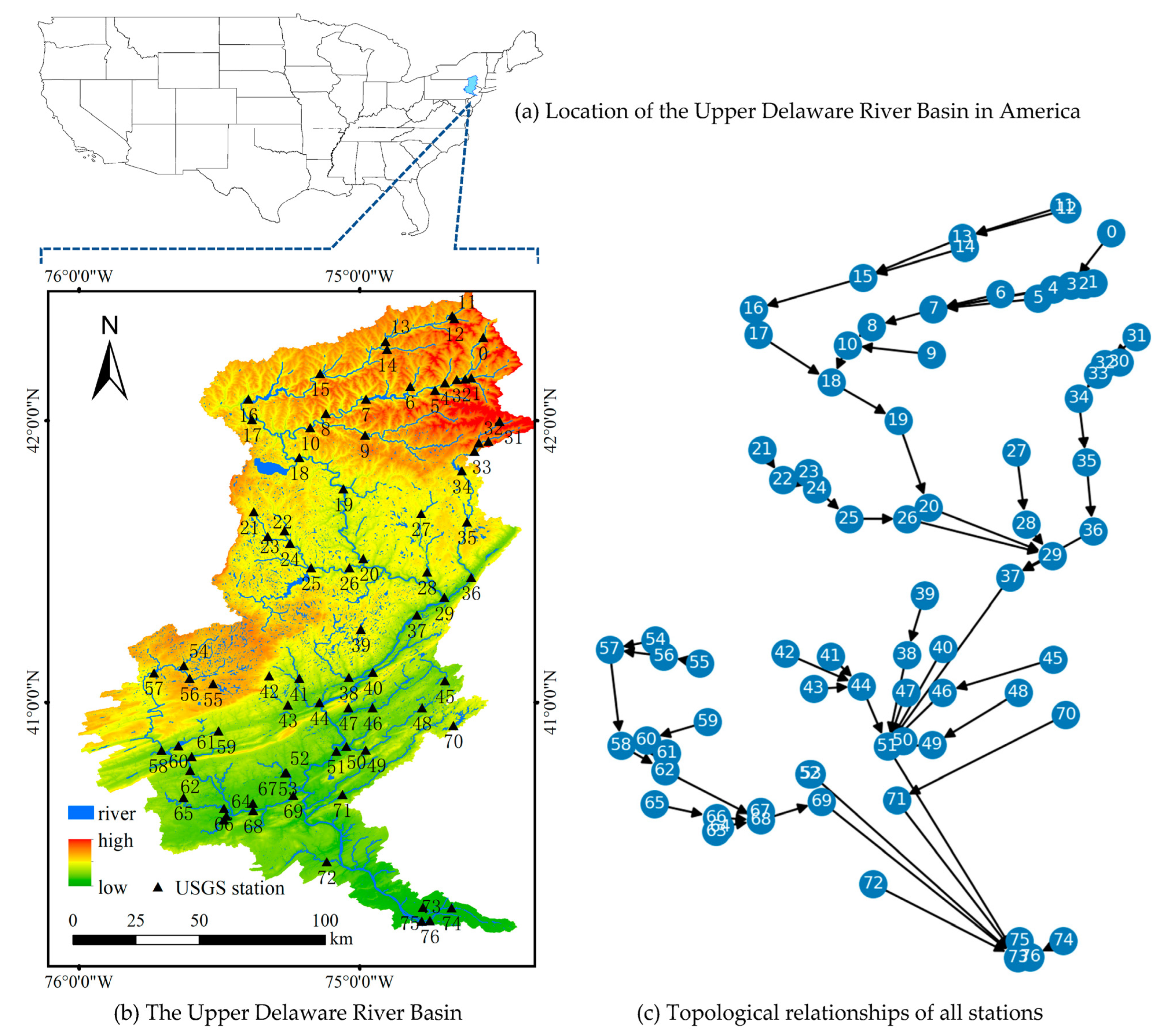
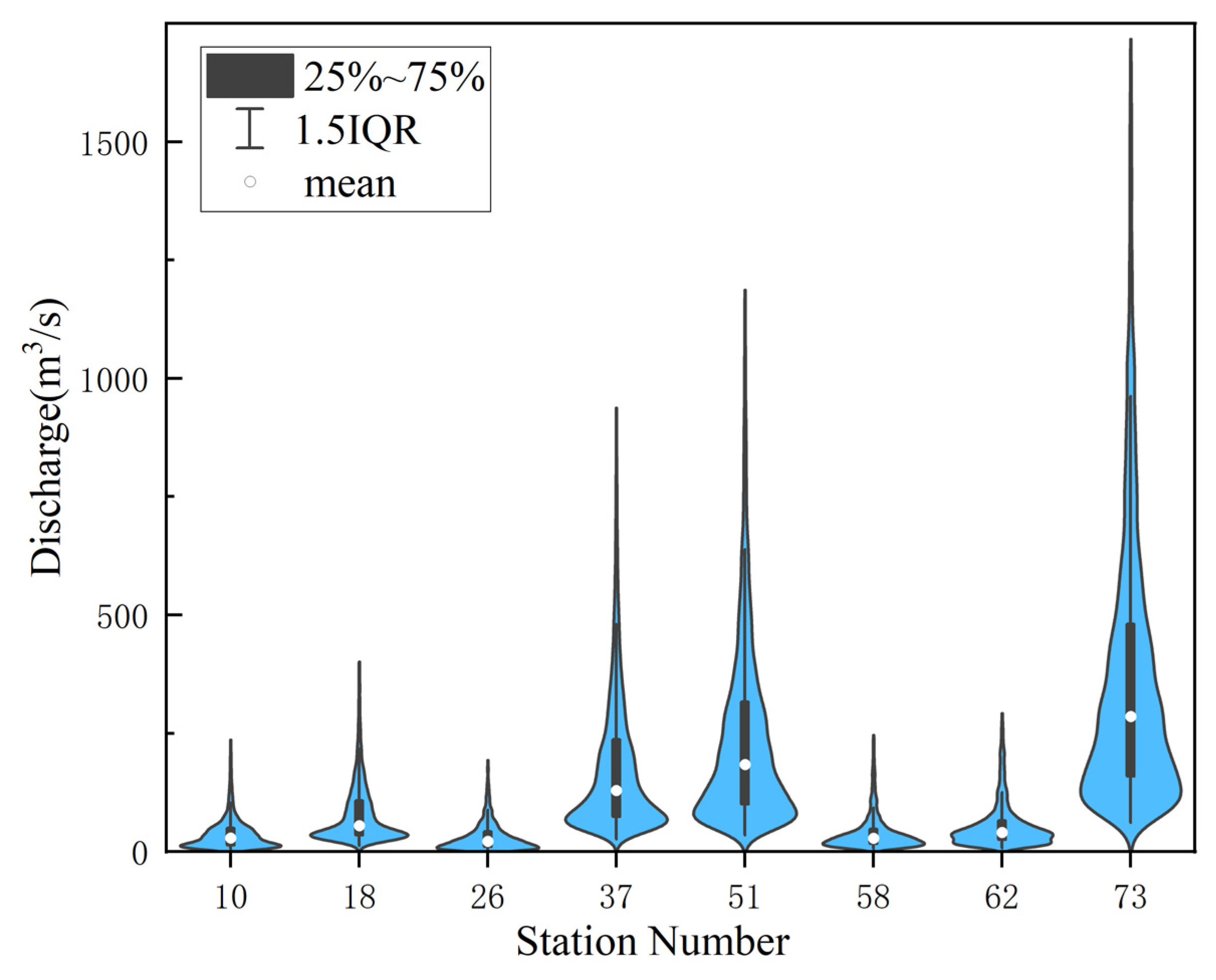
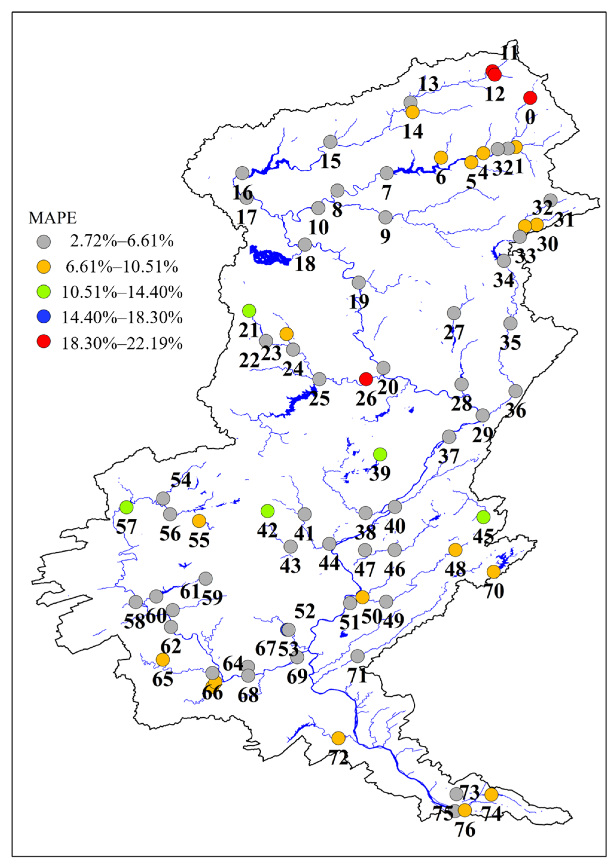
The model in this article is implemented using Pytoch 1.10.0, with a server of Inspur heterogeneous cluster and a graphics card of Tesla V100s with 32G memory. Using the Adam optimization algorithm, set the batch size to 64 and the initial learning rate to 0.002. To prevent overfitting, a dropout [27] rate of 0.1 was used.

4.1. Data Set

To verify the effectiveness of the model presented in this article, 77 hydrological sensors with topological connections were selected from the National Water Information System [28] (NWIS) under the United States Geological Survey (USGS), the Upper Delaware River Basin with HUC code 020401, and their distribution is shown in Figure 5b. Runoff data was collected from 1 January 2016 to 2 January 2021, in a time step of 1 h. Raw runoff data and station data were obtained from NWIS; the watershed data uses the National Hydrology Dataset (NHD) of the United States, and the digital elevation data uses Elevation Products (3DEP). The above datasets are downloaded using the National Map (TNM) service provided by USGS. By importing watershed and site data into ArcGIS, the distance of the river channel is measured. With these stations as the vertices, the adjacency matrix is constructed according to the location relationship between the upstream and downstream of the stations and the river distance. The directed graph of the upstream stations pointing to the downstream stations is shown in Figure 5c, and a complete river network topology is formed from the upstream to the midstream and then to the outlet section of the basin.

The statistical indicators of some stations’ runoff series are shown in Figure 6. The significant differences in runoff at different stations reflect the nonuniformity of spatial distribution, as well as the spatiotemporal distribution heterogeneity caused by the nonuniformity in time distribution, indicating that runoff prediction is a complex spatiotemporal problem.

Use forward padding to fill in missing data for each site runoff sequence. Divide into training, validation, and testing sets at 7:1:2, and use data from the first 24 h to predict future time slices. To accelerate the convergence speed of the model and prevent data leakage, the mean and standard deviation of the training set are used to standardize all data.

4.2. Comparison Model and Evaluation Indicators

In this paper, mean absolute error (MAE), mean squared error (MSE), mean absolute percentage error (MAPE), and Nash–Sutcliffe efficiency coefficient (NSE) are selected to evaluate the performance of the model. The first three indicators are commonly used evaluation indicators for regression tasks, with smaller values indicating smaller errors and better model performance. NSE reflects the goodness of fit between observation and prediction. The range values of NSE is (−∞, 1], and the larger the NSE, the better the model prediction ability.

$$MAE=\frac{1}{m}{\displaystyle \sum _{i=1}^m\left|{\mathit{Y}}_i-{\widehat{\mathit{Y}}}_i\right|}$$

(23)

$$MSE=\frac{1}{m}{\displaystyle \sum _{i=1}^m{\left({\mathit{Y}}_i-{\widehat{\mathit{Y}}}_i\right)}^2}$$

(24)

$$MAPE=\frac{1}{m}{\displaystyle \sum _{i=1}^m\left|\frac{{\mathit{Y}}_i-{\widehat{\mathit{Y}}}_i}{{\mathit{Y}}_i}\right|}$$

(25)

$$NSE=1-\frac{{\displaystyle \sum _{i=1}^m{({\mathit{Y}}_i-{\widehat{\mathit{Y}}}_i)}^2}}{{\displaystyle \sum _{i=1}^m{({\mathit{Y}}_i-\overline{\mathit{Y}})}^2}}$$

(26)

where m represents the time series length, ${\widehat{\mathit{Y}}}_i$ represents the true value, ${\widehat{\mathit{Y}}}_i$ represents the predicted value, and $\overline{\mathit{Y}}$ represents the mean value of the observed values.

The benchmark models are as follows:

(1)

GraphSAGE [29]: It includes sampling and aggregation. First, the neighbors are sampled according to the connection relationship of nodes, and then the information of adjacent nodes is fused together through the aggregate function. Use the fused information to predict node labels.

(2)

GRU: Gated recurrent neural network. The addition of a gating mechanism alleviates the long-term dependency problem of general RNNs.

(3)

DCRNN [30]: In the gating of GRU, graph diffusion convolution is used, which combines temporal and spatial information, and outputs predictive information through the encoder–decoder architecture.

(4)

Graph-WaveNet [31]: Serializing graph convolution and hole convolution to capture spatiotemporal correlation. At the same time, an adaptive adjacency matrix is proposed to capture hidden spatial dependencies.

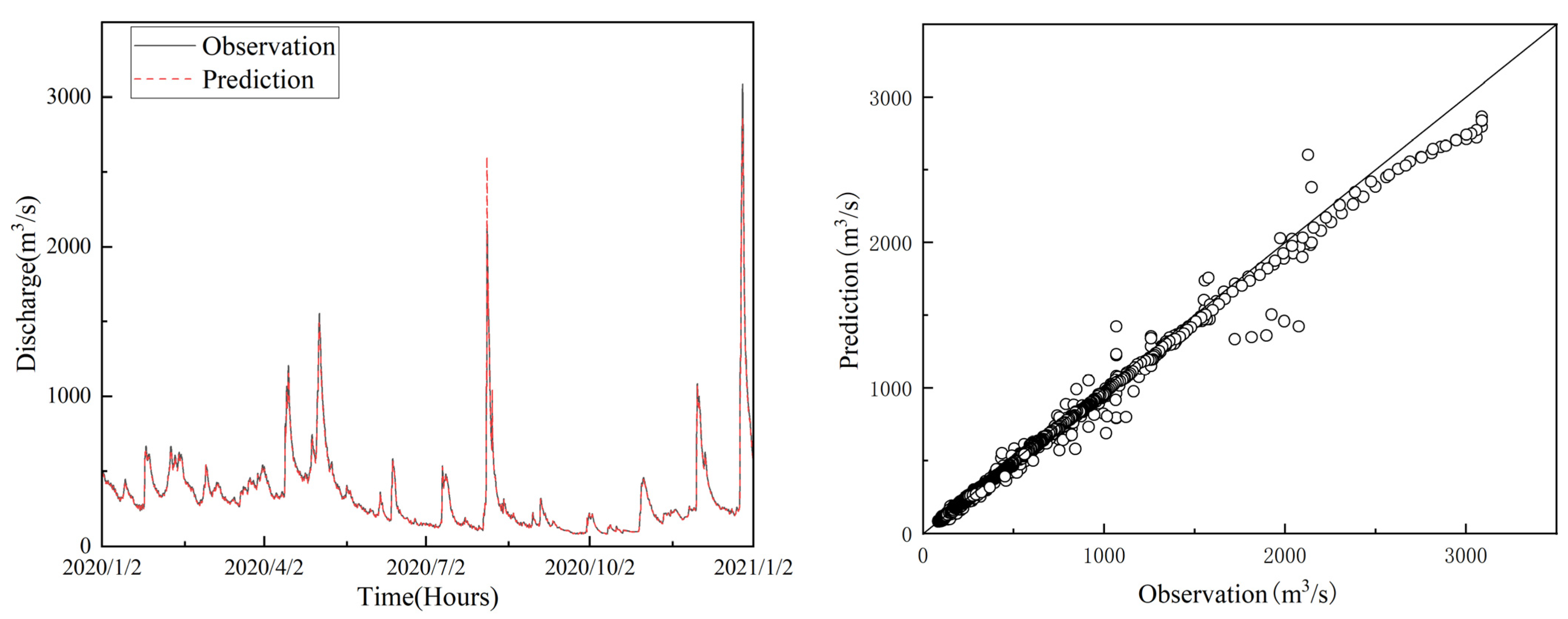
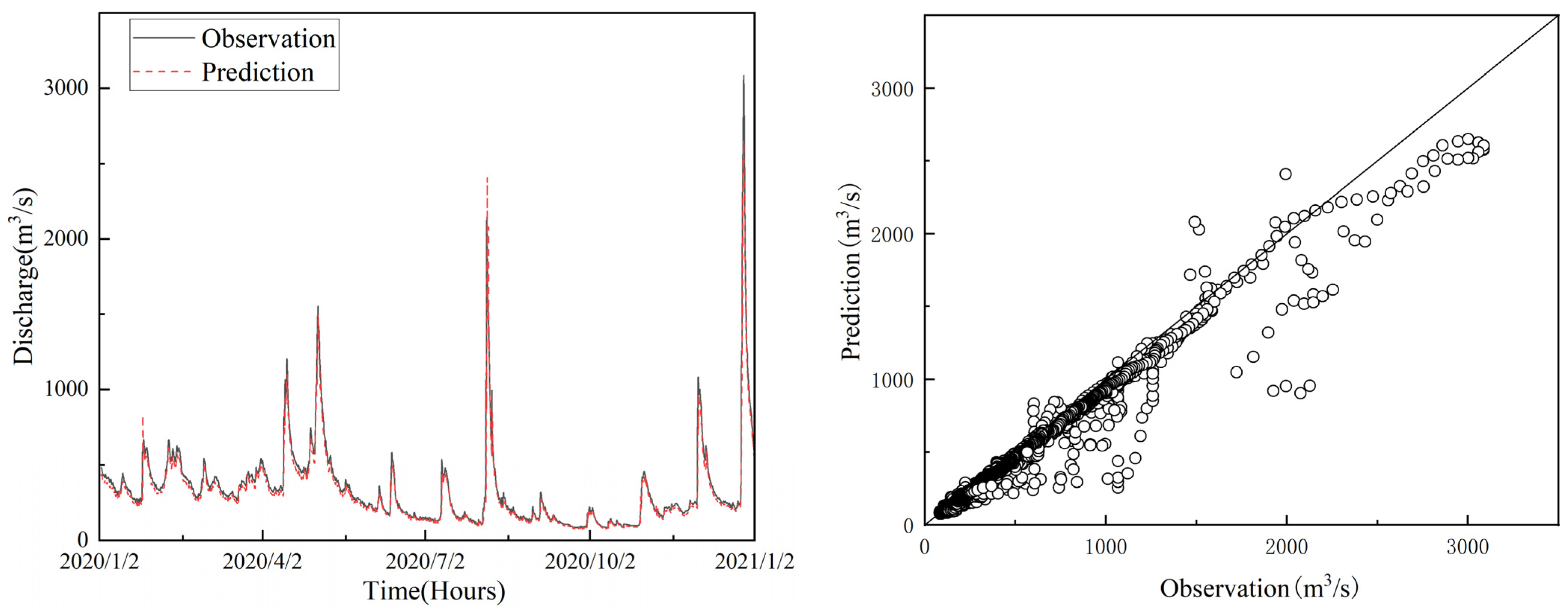
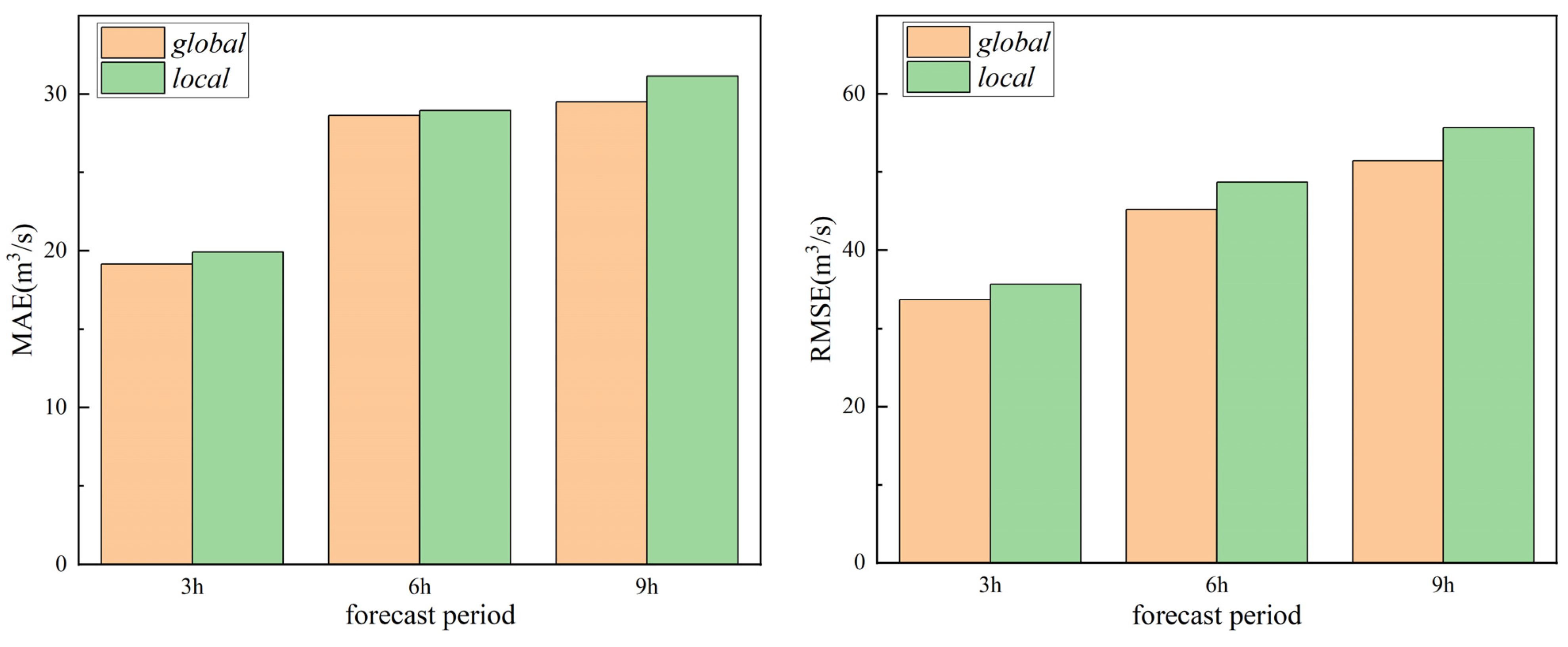
4.3. Result and Analysis

The evaluation index results of the model’s predictive performance are shown in

Table 1. Experiment results.

Methods	3 h				6 h				9 h
	MAE	MSE	MAPE	NSE	MAE	MSE	MAPE	NSE	MAE	MSE	MAPE	NSE
GraphSAGE	1.27	8.76	6.01%	0.83	2.57	15.73	9.87%	0.74	3.09	21.58	11.83%	0.61
GRU	1.22	6.54	5.45%	0.85	2.21	9.24	9.12%	0.76	2.79	12.66	10.51%	0.62
DCRNN	1.10	5.69	5.38%	0.89	2.15	8.61	8.15%	0.79	2.81	11.53	10.34%	0.68
Graph-WaveNet	1.07	5.67	5.21%	0.89	2.07	8.21	7.64%	0.80	2.73	10.33	9.01%	0.67
DSTGNN	1.05	4.92	5.11%	0.90	2.03	7.70	6.97%	0.83	2.71	9.37	8.52%	0.71

. In MAE, MSE, MAP, and NSE, this model improves by 2.03%, 6.21%, 0.67%, and 0.03 over the current state-of-the-art models. This model outperforms the benchmark model in all indicators, confirming its feasibility and effectiveness. The specific analysis is as follows:

(1)

Spatiotemporal fusion has a large improvement on the prediction performance. The performance index of GRU with temporal modeling is better than that of GraphSAGE with spatial modeling, indicating that the sequence model has advantages in temporal prediction. Compared with GRU, which only considers a single time-series dependence, the model in this paper extracts the topological relationship of the basin and exploits the spatial and temporal dependence of the flow at upstream and downstream hydrological stations, so the accuracy is greatly improved.

(2)

The attention mechanism has improved the performance of long-time prediction. The robustness and generalization of all models gradually deteriorate as the prediction step length increases. In this paper, the performance of the long-term prediction model is improved by introducing the attention mechanism to mine the potential patterns of the time series, while incorporating multiple upstream site features and considering the time lag.

In order to visually display the prediction results of this model, Figure 7, Figure 8 and Figure 9 show the visualization results of the watershed outlet station 73 under different foresight periods. From the figure, it can be seen that the model fits the runoff process well. When the foresight period is 3 h, the deviation between the predicted value and the true value is not significant. As the foresight period increases, the performance of the model decreases significantly and the degree of deviation increases. In addition, the simulation accuracy of the model under low runoff conditions is much higher than that under high runoff conditions. The model underestimates the influence of discrete values to achieve better overall performance, which is an area that needs improvement in future work.

Figure 10 shows the spatial distribution of the average MAPE of different sites during the forecasting period, and shows that the error of more than 60% of the stations is located in the interval of 2.72–6.61%, and the MAPE of nearly 90% of the stations is within 10.51%, indicating that the model is accurate in predicting most of the sites. The stations with larger errors are generally located in the upstream area, which is because the runoff in the upstream area is smaller and more disturbed by human and natural factors, making prediction more difficult.

In order to verify the effectiveness of the proposed module, ablation experiments were carried out in this paper. The adjacency matrix was used to replace the distance weight matrix to obtain the control model w/o static, the dynamic matrix was removed to obtain the w/o dynamic, and the spatial block was removed to obtain the w/o spatial. Compared with the original model, the experimental results are shown in

Table 2. Result of ablation experiment.

Model	MAE	MSE	MAPE
w/o static	1.93	9.54	9.50%
w/o dynamic	1.95	9.64	9.55%
w/o spatial	1.97	10.61	10.05%
full	1.91	9.37	8.52%

. The performance of the complete model is better than the control model. The ablation experiment has demonstrated the importance of spatial modeling for multi-station runoff prediction within a basin, as well as the importance of the distance weight matrix and dynamic graph matrix used in this paper for improving model performance.

Considering the different distribution of stations in different watersheds, local stations are used as comparison experiments to verify the robustness of the model proposed in this paper. The control experiment is modeled only with the watershed outlet station 73 and its first-order neighbors 51, 53, 69, 71, 72, and 76. The RMSE results for station 73 with different context information are shown in Figure 11, and the error is reduced by about 6 percentage points with global information. Global modeling is more conducive to mining the watershed characteristics and improving prediction accuracy.

5. Conclusions

In this paper, a graph convolutional network model incorporating spatiotemporal features is proposed for runoff prediction. First, the topology of the river network is abstracted into a graph structure, and the corresponding adjacency matrix is constructed for the unidirectional mobility and time-varying characteristics of the water flow. After that, the spatial and temporal dependencies are captured by graph convolutional network and LSTM with the self-attention mechanism, respectively. Finally, the gating mechanism is used to fuse the features of these two different dimensions, and the representation capability of the model is enhanced after the multi-layer stacking. Experiments are conducted in a realistic basin to verify the validity of the model, which outperforms the comparison model in MAE, MSE, MAPE, and NSE metrics. Finally, the effectiveness of the proposed weighted distance matrix, dynamic matrix, and both spatial and temporal blocks in improving the accuracy of the model is demonstrated by ablation experiments; the spatial block and the two matrices reflect the river network confluence mechanism, whereas the temporal block corresponds to the flow production mechanism.

The model proposed in this paper can effectively predict future runoff flows, but has the following shortcomings that can be used as a direction for subsequent research:

(1)

The simulation accuracy of the model is much higher at low flows than at high flows, and the model underestimates the effect of discrete values to make the overall performance better. If the model can predict the abrupt change point of the flow sequence in advance, it can undoubtedly improve the prediction accuracy under a high flow rate, which is an area that needs to be improved in future work.

(2)

In the subsequent research, this paper needs to consider more physical factors of the water cycle and combine relevant domain knowledge in the model to enhance the accuracy and physical interpretability of the model; secondly, it is necessary to combine the relevant research results of distributed hydrological models and introduce fine subsurface characteristics, such as soil type and surface plant cover, into the model.

References

1. Zhang, X.; Deng, L.; Wu, B.; Gao, S.; Xiao, Y. Low-Impact Optimal Operation of a Cascade Sluice-Reservoir System for Water-Society-Ecology Trade-Offs. Water Resour. Manag. 2022, 36, 6131–6148. [Google Scholar] [CrossRef]
2. Nourani, V.; Baghanam, A.H.; Adamowski, J.; Kisi, O. Applications of hybrid wavelet–Artificial Intelligence models in hydrology: A review. J. Hydrol. 2014, 514, 358–377. [Google Scholar] [CrossRef]
3. LeCun, Y.; Bengio, Y.; Hinton, G. Deep learning. Nature 2015, 521, 436–444. [Google Scholar] [CrossRef]
4. Shen, C. A Transdisciplinary Review of Deep Learning Research and Its Relevance for Water Resources Scientists. Water Resour. Res. 2018, 54, 8558–8593. [Google Scholar] [CrossRef]
5. Lv, N.; Liang, X.; Chen, C.; Zhou, Y.; Li, J.; Wei, H.; Wang, H. A long Short-Term memory cyclic model with mutual information for hydrology forecasting: A Case study in the xixian basin. Adv. Water Resour. 2020, 141, 10. [Google Scholar] [CrossRef]
6. Tao, L.; He, X.; Li, J.; Yang, D. A multiscale long short-term memory model with attention mechanism for improving monthly precipitation prediction. J. Hydrol. 2021, 602, 13. [Google Scholar] [CrossRef]
7. Wang, H.; Qin, H.; Liu, G.; Liu, S.; Qu, Y.; Wang, K.; Zhou, J. A novel feature attention mechanism for improving the accuracy and robustness of runoff forecasting. J. Hydrol. 2023, 618, 129200. [Google Scholar] [CrossRef]
8. Xie, Y.; Sun, W.; Ren, M.; Chen, S.; Huang, Z.; Pan, X. Stacking ensemble learning models for daily runoff prediction using 1D and 2D CNNs. Expert Syst. Appl. 2023, 217, 119469. [Google Scholar] [CrossRef]
9. Zhao, X.; Lv, H.; Wei, Y.; Lv, S.; Zhu, X. Streamflow Forecasting via Two Types of Predictive Structure-Based Gated Recurrent Unit Models. Water 2021, 13, 91. [Google Scholar] [CrossRef]
10. Khadr, M.; Schlenkhoff, A. GA-based implicit stochastic optimization and RNN-based simulation for deriving multi-objective reservoir hedging rules. Environ. Sci. Pollut. Res. 2021, 28, 19107–19120. [Google Scholar] [CrossRef]
11. Qiu, R.; Wang, Y.; Wang, D.; Qiu, W.; Wu, J.; Tao, Y. Water temperature forecasting based on modified artificial neural network methods: Two cases of the Yangtze River. Sci. Total Environ. 2020, 737, 12. [Google Scholar] [CrossRef] [PubMed]
12. Bai, Y.; Chen, Z.; Xie, J.; Li, C. Daily reservoir inflow forecasting using multiscale deep feature learning with hybrid models. J. Hydrol. 2016, 532, 193–206. [Google Scholar] [CrossRef]
13. Li, F.; Ma, G.; Chen, S.; Huang, W. An Ensemble Modeling Approach to Forecast Daily Reservoir Inflow Using Bidirectional Long- and Short-Term Memory (Bi-LSTM), Variational Mode Decomposition (VMD), and Energy Entropy Method. Water Resour. Manag. 2021, 35, 2941–2963. [Google Scholar] [CrossRef]
14. Huang, S.; Yu, L.; Luo, W.; Pan, H.; Li, Y.; Zou, Z.; Wang, W.; Chen, J. Runoff Prediction of Irrigated Paddy Areas in Southern China Based on EEMD-LSTM Model. Water 2023, 15, 1704. [Google Scholar] [CrossRef]
15. Gori, M.; Monfardini, G.; Scarselli, F. A new model for learning in graph domains. In Proceedings of the 2005 IEEE International Joint Conference on Neural Networks, Montreal, QC, Canada, 31 July–4 August 2005; pp. 729–734. [Google Scholar]
16. Wang, Y.; Wang, H.; Jin, H.; Huang, X.; Wang, X. Exploring graph capsual network for graph classification. Inf. Sci. 2021, 581, 932–950. [Google Scholar] [CrossRef]
17. Chang, J.X.; Gao, C.; Zheng, Y.; Hui, Y.Q.; Niu, Y.A.; Song, Y.; Jin, D.P.; Li, Y. Sequential Recommendation with Graph Neural Networks. In Proceedings of the Sigir 21—Proceedings of the 44th International Acm Sigir Conference on Research and Development in Information Retrieval, Virtual, 11–15 July 2021; pp. 378–387. [Google Scholar] [CrossRef]
18. Zhao, T.; Hu, Y.; Valsdottir, L.R.; Zang, T.; Peng, J. Identifying drug–target interactions based on graph convolutional network and deep neural network. Brief. Bioinform. 2021, 22, 2141–2150. [Google Scholar] [CrossRef]
19. Deng, A.L.; Hooi, B. Graph Neural Network-Based Anomaly Detection in Multivariate Time Series. Proc. AAAI Conf. Artif. Intell. 2021, 35, 4027–4035. [Google Scholar] [CrossRef]
20. Sun, A.Y.; Jiang, P.; Yang, Z.-L.; Xie, Y.; Chen, X. A graph neural network (GNN) approach to basin-scale river network learning: The role of physics-based connectivity and data fusion. Hydrol. Earth Syst. Sci. 2022, 26, 5163–5184. [Google Scholar] [CrossRef]
21. Liu, G.; Ouyang, S.; Qin, H.; Liu, S.; Shen, Q.; Qu, Y.; Zheng, Z.; Sun, H.; Zhou, J. Assessing spatial connectivity effects on daily streamflow forecasting using Bayesian-based graph neural network. Sci. Total Environ. 2023, 855, 158968. [Google Scholar] [CrossRef]
22. Xiang, Z.; Demir, I. Fully distributed rainfall-runoff modeling using spatial-temporal graph neural network. EarthArXiv 2022. [Google Scholar] [CrossRef]
23. Hochreiter, S.; Schmidhuber, J. Long short-term memory. Neural Comput. 1997, 9, 1735–1780. [Google Scholar] [CrossRef] [PubMed]
24. Vaswani, A.; Shazeer, N.; Parmar, N.; Uszkoreit, J.; Jones, L.; Gomez, A.N.; Kaiser, L.; Polosukhin, I. Attention Is All You Need. In Proceedings of the Advances in Neural Information Processing Systems 30 (NIPS 2017), Long Beach, CA, USA, 4–9 December 2017. [Google Scholar]
25. Wang, X.; Ma, Y.; Wang, Y.; Jin, W.; Wang, X.; Tang, J.; Jia, C.; Yu, J. Traffic flow prediction via spatial temporal graph neural network. In Proceedings of the Web Conference 2020, Taipei, Taiwan, 20–24 April 2020; pp. 1082–1092. [Google Scholar]
26. Oreshkin, B.N.; Carpov, D.; Chapados, N.; Bengio, Y. N-BEATS: Neural basis expansion analysis for interpretable time series forecasting. arXiv 2019, arXiv:1905.10437. [Google Scholar]
27. Srivastava, N.; Hinton, G.; Krizhevsky, A.; Sutskever, I.; Salakhutdinov, R. Dropout: A simple way to prevent neural networks from overfitting. J. Mach. Learn. Res. 2014, 15, 1929–1958. [Google Scholar]
28. De Cicco, L.; Lorenz, D.; Hirsch, R.; Watkins, W.; Johnson, M. dataRetrieval: R Packages for Discovering and Retrieving Water Data Available from US Federal Hydrologic Web Services; US Geological Survey: Reston, VA, USA, 2022. [CrossRef]
29. Hamilton, W.; Ying, Z.; Leskovec, J. Inductive representation learning on large graphs. In Proceedings of the Advances in Neural Information Processing Systems 30 (NIPS 2017), Long Beach, CA, USA, 4–9 December 2017. [Google Scholar]
30. Li, Y.; Yu, R.; Shahabi, C.; Liu, Y. Diffusion convolutional recurrent neural network: Data-driven traffic forecasting. arXiv 2017, arXiv:1707.01926. [Google Scholar]
31. Wu, Z.H.; Pan, S.R.; Long, G.D.; Jiang, J.; Zhang, C.Q. Graph WaveNet for Deep Spatial-Temporal Graph Modeling. In Proceedings of the 28th International Joint Conference on Artificial Intelligence, Macao, China, 10–16 August 2019; pp. 1907–1913. [Google Scholar]
Figure 1. Spatial-temporal correlation between upstream and downstream stations.
Water 15 02463 g001
Figure 2. DSTGNN model.
Water 15 02463 g002
Figure 3. Temporal block, LSTM with the self-attention mechanism.
Water 15 02463 g003
Figure 4. Pearson correlation coefficient of the runoff sequence of all stations in the basin.
Water 15 02463 g004
Figure 5. Study area. (a) Location of the Upper Delaware River Basin in America; (b) the Upper Delaware River Basin. (c) Topological relationships of all stations.
Water 15 02463 g005
Figure 6. Violin plot of the observed runoff times series.
Water 15 02463 g006
Figure 7. The runoff prediction and goodness-of-fit at 3 h ahead in the testing period.
Water 15 02463 g007
Figure 8. The runoff prediction and goodness-of-fit at 6 h ahead in the testing period.
Water 15 02463 g008
Figure 9. The runoff prediction and goodness-of-fit at 9 h ahead in the testing period.
Water 15 02463 g009
Figure 10. Spatial distribution of MAPE.
Water 15 02463 g010
Figure 11. Impact of different contextual information.
Water 15 02463 g011