Development of a Three-Dimensional Hydrodynamic Model Based on the Discontinuous Galerkin Method

Abstract

Though the discontinuous Galerkin method is attracting more and more applications in many fields due to its local conservation, high-order accuracy, and flexibility for resolving complex geometries, only a few three-dimensional hydrodynamic models based on the discontinuous Galerkin method are present. In this study, a three-dimensional hydrodynamic model with a σ-coordinate system in the vertical direction is developed. This model is discretized in space using the discontinuous Galerkin method and advanced in time with the implicit-explicit Runge–Kutta method. Numerical tests indicate that the developed model is convergent and can obtain better results with a smaller computational time when a higher approximation order is adopted. Other tests with exact solutions also indicate that the developed model can well simulate the vertical circulation under the effect of surface wind stress and the flow under the combined effect of wind stress and Coriolis acceleration terms. The simulation results of tidal flow in part of Bohai Bay, China, indicate that the model can be used for the simulation of tidal wave motion in realistic situations.

1. Introduction

With the assumption of hydrostatic pressure distribution, the three-dimensional shallow water equations (3D SWEs) can be derived from the Reynolds-averaged three-dimensional Navier–Stokes equations. They can predict the vertical distribution of primitive variables and can be used together with advection-diffusion-type equations to simulate the transport and fate of substances, such as temperature, salt, and sediment.

In the last few decades, 3D SWEs have been intensively studied [1], and many hydrodynamic models have been developed and widely used. A brief categorization of these models, based on the numerical methods and the type of grids used in the horizontal direction, is listed in Table 1. For the models at an early stage, the conservative finite difference method on structured grids was usually used. They can be implemented straightforwardly and are computationally efficient, while they approximate the coastlines as staircases and prevent the flexible implementation of variable resolution. Later, unstructured, grid-based hydrodynamic models, such as the finite element and finite volume method, were brought into the main stream, since the coastlines could be accurately represented to give a reasonable simulation at the regional scale [2], and the area of most concern could be simulated using local refinement grids.

In addition to the numerical methods mentioned above, the discontinuous Galerkin (DG) method has received much attention in recent years. It can be viewed as a hybrid between the finite element method and the finite volume method and enjoys most of the strengths of both methods, such as local conservation, compactness, a high order of accuracy, and good application to unstructured meshes. It has been successfully applied in the numerical discretization of two-dimensional shallow water equations [3], two-dimensional non-hydrostatic shallow water equations [4], and Boussinesq-type equations [5].

Table 1. Categorization of the commonly used hydrodynamic model.

Grid Type	Numerical Method
	Finite Difference Method	Finite Volume Method	Finite Element Method
Structured grid	ROMS [6], POM [7], MoM [8], GETM [9], TRIM [10], DELFT3D [11], EFDC [12], ECOMSED [13], COHERENS [14]	MITgcm [15], MOHID [16]
Unstructured grid		FVCOM [17], UnTRIM [18], HydroInfo [19]	FESOM [20], ICOM, SELFE [21], ADCIRC [22], SCHISM [23], TELEMAC [24]

Table 1. Categorization of the commonly used hydrodynamic model.

Grid Type	Numerical Method
	Finite Difference Method	Finite Volume Method	Finite Element Method
Structured grid	ROMS [6], POM [7], MoM [8], GETM [9], TRIM [10], DELFT3D [11], EFDC [12], ECOMSED [13], COHERENS [14]	MITgcm [15], MOHID [16]
Unstructured grid		FVCOM [17], UnTRIM [18], HydroInfo [19]	FESOM [20], ICOM, SELFE [21], ADCIRC [22], SCHISM [23], TELEMAC [24]

In the realm of 3D SWEs with DG solutions, Dawson and Aizinger [25] first developed a three-dimensional barotropic model with a z-coordinate system adopted in the vertical direction and presented the corresponding stability analysis [26]. The vertical eddy viscosity terms in the model are explicitly advanced in time. Due to the stiffness of these terms, the time step must be small enough, which limits the applicability of the model. Later, Aizinger et al. [27] made improvements by introducing the baroclinic terms and treating both the vertical eddy viscosity and the vertical diffusion terms implicitly. This model is called UTBEST3D and has been validated with realistic applications. In the same period, Blaise [28] and Comblen [29] developed the three-dimensional baroclinic model named SLIM and adopted it for the simulation of various baroclinic phenomena. Due to the discontinuous nature of the DG method, the water depth between the adjacent elements is generally not continuous such that the lateral boundaries are mismatched, and the post-process measures are needed to smooth the water depth such that the calculation of numerical flux will not be affected. To circumvent the problem of boundary mismatch between adjacent elements, Gandham [30] mapped the time-varying z-coordinate system to a fixed domain by invoking the σ-coordinate transformation and developed a three-dimensional barotropic model. However, only one layer is adopted in the vertical direction, which may lead to serious numerical errors when the water depth is large. Conroy and Kubatko [31] developed a three-dimensional barotropic model with a σ-coordinate system adopted in the vertical direction and developed a fast and accurate method for the calculation of depth-averaged velocity. An arbitrary number of layers can be used in the vertical direction. However, non-linear advective terms are not included, and the vertical eddy viscosity terms are explicitly advanced in time. To the authors’ knowledge, there is currently no DG method-based three-dimensional hydrodynamic model that includes non-linear advective terms, treats the vertical eddy viscosity terms implicitly, and can use an arbitrary number of vertical layers in the σ-coordinate system simultaneously.

In this paper, a three-dimensional hydrodynamic model that includes nonlinear advective terms and can use an arbitrary number of vertical layers in the σ-coordinate system is developed based on the DG method. The paper is organized as follows. In Section 2, we provide the governing equations of the 3D SWEs in the σ-coordinate system. Then, we present the space discretization and time stepping of the model in Section 3. Numerical experiments are given in Section 4. Finally, conclusions are drawn in Section 5.

2. Governing Equations

Using the notations given in Table 2, the governing equations of the three-dimensional hydrodynamic model in the physical domain are as follows [13]:

$$\frac{\partial u}{\partial x}+\frac{\partial v}{\partial y}+\frac{\partial w}{\partial z}=0,$$

(1)

$$\frac{\partial u}{\partial t}+\frac{\partial \left(uu\right)}{\partial x}+\frac{\partial \left(uv\right)}{\partial y}+\frac{\partial \left(uw\right)}{\partial z}-fv=-g\frac{\partial \eta }{\partial x}+\frac{\partial }{\partial z}\left(K_m\frac{\partial u}{\partial z}\right)+\frac{\partial }{\partial x}\left(K_h\frac{\partial u}{\partial x}\right)+\frac{\partial }{\partial y}\left(K_h\frac{\partial u}{\partial y}\right),$$

(2)

$$\frac{\partial v}{\partial t}+\frac{\partial \left(uv\right)}{\partial x}+\frac{\partial \left(vv\right)}{\partial y}+\frac{\partial \left(vw\right)}{\partial z}+fu=-g\frac{\partial \eta }{\partial y}+\frac{\partial }{\partial z}\left(K_m\frac{\partial v}{\partial z}\right)+\frac{\partial }{\partial x}\left(K_h\frac{\partial v}{\partial x}\right)+\frac{\partial }{\partial y}\left(K_h\frac{\partial v}{\partial y}\right),$$

(3)

Table 2. Notations for the governing equations of the three-dimensional hydrodynamic model.

Variables	Explanation
$u\left(x,y,z,t\right)$	velocity of water in x direction
$v\left(x,y,z,t\right)$	velocity of water in y direction
$w\left(x,y,z,t\right)$	velocity of water in z direction
g	acceleration due to gravity
$\theta$	angle of geographical latitude
$\varpi$	magnitude of the angular velocity of the Earth
$f=2\varpi \sin \theta$	Coriolis parameter
$K_m$	vertical eddy viscosity coefficient
$K_h$	horizontal eddy viscosity coefficient
${\rho }_0$	density
${\tau }_{sx}$	wind stress in x direction
${\tau }_{sy}$	wind stress in y direction
$\eta \left(x,y,t\right)$	the surface elevation
$u_{\eta }\left(x,y,t\right)$	surface velocity of water in x direction
$v_{\eta }\left(x,y,t\right)$	surface velocity of water in y direction
$b\left(x,y\right)$	bottom elevation
$u_b\left(x,y,t\right)$	bottom velocity of water in x direction
$v_b\left(x,y,t\right)$	bottom velocity of water in y direction
$z_0\left(x,y,t\right)$	half height of the bottommost element
$u_c\left(x,y,t\right)$	$\mathrm{velocity} \mathrm{of} \mathrm{water} \mathrm{at} z_0$ in x direction
$v_c\left(x,y,t\right)$	$\mathrm{velocity} \mathrm{of} \mathrm{water} \mathrm{at} z_0$ in y direction
$C_f\left(x,y,t\right)$	drag coefficient
$\kappa$	von Karman constant
$z_0^b\left(x,y\right)$	bottom roughness parameter
$\omega \left(x,y,\sigma ,t\right)$	vertical velocity in the computational domain
$\overline{U}\left(x,y,t\right)$	depth-averaged velocity in x direction
$\overline{V}\left(x,y,t\right)$	depth-averaged velocity in y direction
$D\left(x,y,t\right)=\eta \left(x,y,t\right)-b\left(x,y\right)$	water depth

The surface boundary conditions for $u$, $v$, and $w$ are

$$\left(K_m\frac{\partial u}{\partial z},K_m\frac{\partial v}{\partial z}\right)=\frac{1}{{\rho }_0}\left({\tau }_{sx},{\tau }_{sy}\right),$$

(4)

$$w=\frac{\partial \eta }{\partial t}+u_{\eta }\frac{\partial \eta }{\partial x}+v_{\eta }\frac{\partial \eta }{\partial y}.$$

(5)

Likewise, the bottom boundary conditions for $u$, $v$, and $w$ are

$$w=u_b\frac{\partial b}{\partial x}+v_b\frac{\partial b}{\partial y},$$

(6)

$$\left(K_m\frac{\partial u}{\partial z},K_m\frac{\partial v}{\partial z}\right)=C_f\sqrt{u_c^2+v_c^2}\left(u_c,v_c\right),$$

(7)

where $C_f$ is determined by matching a logarithmic bottom layer to the model at height $z_0$ and calculated as [32]

$$C_f={\left(\frac{\kappa }{\ln \left(\left(z_0+z_0^b\right)/z_0^b\right)}\right)}^2.$$

(8)

To accurately represent the bottom and surface geometry, the $\sigma$ transformation developed by Philips [33] is adapted

$$t^{*}=t,x^{*}=x,y^{*}=y,\sigma =\frac{z-\eta \left(x,y,t\right)}{D\left(x,y,t\right)}.$$

(9)

According to the principle of chain differentiation, partial derivatives of the variable $\zeta =\zeta (x,y,z,t)$ in the physical domain can be written in the following form in the computational domain:

$$\begin{array}{l}\frac{\partial \zeta }{\partial t}=\frac{\partial \zeta }{\partial t^{*}}+\frac{\partial \zeta }{\partial \sigma }\frac{\partial \sigma }{\partial t},\\ \frac{\partial \zeta }{\partial x}=\frac{\partial \zeta }{\partial x^{*}}+\frac{\partial \zeta }{\partial \sigma }\frac{\partial \sigma }{\partial x},\\ \frac{\partial \zeta }{\partial y}=\frac{\partial \zeta }{\partial y^{*}}+\frac{\partial \zeta }{\partial \sigma }\frac{\partial \sigma }{\partial y},\\ \frac{\partial \zeta }{\partial z}=\frac{\partial \zeta }{\partial \sigma }\frac{\partial \sigma }{\partial z}.\end{array}$$

(10)

Substituting Equation (10) back into Equations (1)–(3), and ignoring the superscript “*”, we can obtain the governing equations in the computational domain as

$$\frac{\partial D}{\partial t}+\frac{\partial \left(Du\right)}{\partial x}+\frac{\partial \left(Dv\right)}{\partial y}+\frac{\partial \omega }{\partial \sigma }=0,$$

(11)

$$\frac{\partial U}{\partial t}+\frac{\partial E}{\partial x}+\frac{\partial G}{\partial y}+\frac{\partial H}{\partial \sigma }=S_0+S_f+S_{d,v}+S_{d,h}.$$

(12)

with

$$U=\left[\begin{array}{c}Du\\ Dv\end{array}\right], E=\left[\begin{array}{c}D{u}^2+1/2\left(g\left(D^2-z_b^2\right)\right)\\ Duv\end{array}\right], G=\left[\begin{array}{c}Duv\\ D{v}^2+1/2\left(g\left(D^2-z_b^2\right)\right)\end{array}\right], H=\left[\begin{array}{c}\omega u\\ \omega v\end{array}\right].$$

(13)

$$S_0=\left[\begin{array}{c}-g\eta \partial z_b/\partial x\\ -g\eta \partial z_b/\partial y\end{array}\right], S_f=\left[\begin{array}{c}-fDv\\ fDu\end{array}\right].$$

(14)

$$S_{d,v}=\left[\begin{array}{c}\frac{\partial }{\partial \sigma }\left(\frac{K_m}{D^2}\frac{\partial \left(Du\right)}{\partial \sigma }\right)\\ \frac{\partial }{\partial \sigma }\left(\frac{K_m}{D^2}\frac{\partial \left(Dv\right)}{\partial \sigma }\right)\end{array}\right], S_{d,h}=\left[\begin{array}{c}\frac{\partial }{\partial x}\left(K_{h}D\frac{\partial u}{\partial x}\right)+\frac{\partial }{\partial y}\left(K_{h}D\frac{\partial u}{\partial y}\right)\\ \frac{\partial }{\partial x}\left(K_{h}D\frac{\partial v}{\partial x}\right)+\frac{\partial }{\partial y}\left(K_{h}D\frac{\partial v}{\partial y}\right)\end{array}\right].$$

(15)

where $\omega$ is related to $w$ by

$$\omega =D\frac{d\sigma }{dt}=w-\left(\frac{\partial z_s}{\partial t}+\sigma \frac{\partial D}{\partial t}\right)-u\left(\frac{\partial z_s}{\partial x}+\sigma \frac{\partial D}{\partial x}\right)-v\left(\frac{\partial z_s}{\partial y}+\sigma \frac{\partial D}{\partial y}\right).$$

(16)

The surface boundary condition in the computational domain is given by

$$\begin{array}{l}\omega =0,\\ \left(\frac{K_m}{D^2}\frac{\partial \left(Du\right)}{\partial \sigma },\frac{K_m}{D^2}\frac{\partial \left(Dv\right)}{\partial \sigma }\right)=\frac{1}{{\rho }_0}\left({\tau }_{sx},{\tau }_{sy}\right),\end{array}$$

(17)

and the bottom boundary condition is given by

$$\begin{array}{l}\omega =0,\\ \left(\frac{K_m}{D^2}\frac{\partial \left(Du\right)}{\partial \sigma },\frac{K_m}{D^2}\frac{\partial \left(Dv\right)}{\partial \sigma }\right)=C_f\sqrt{u_b^2+v_b^2}\left(u_b,v_b\right),\end{array}$$

(18)

Integrating Equation (11) from bottom to surface and applying the boundary condition about $\omega$ leads to the primitive continuity equation as

$$\frac{\partial D}{\partial t}+\frac{\partial \left(D\overline{U}\right)}{\partial x}+\frac{\partial \left(D\overline{V}\right)}{\partial y}=0$$

(19)

3. Numerical Implementation

In this section, we will detail the numerical implementation of our model based on the DG method. The domain partition and the discontinuous polynomial space are first described. Then, the numerical discretization of each part is presented, followed by the time-stepping scheme.

3.1. Domain Partition and Polynomial Space

For an arbitrary three-dimensional domain ${\Omega }_{3d}$, its horizontal projection is denoted as ${\Omega }_{2d}$ and is partitioned by $Ele2d$ non-overlapping triangular or quadrilateral elements; i.e., ${\Omega }_{2d,h}=\left\{{\Omega }_e\right\},e\in \left[1,Ele2d\right]$. In the vertical direction, ${\Omega }_{2d,h}$ is extruded by $N_L$ layers to obtain the three-dimensional computational domain ${\Omega }_{3d,h}$, and the computational domain consists of $Ele2d\times N_L$ triangular prisms or quadrangular prisms. In this study, the three-dimensional element obtained by the extrusion of ${\Omega }_e$ is denoted as ${\Omega }_{\left(e,L\right)},L\in \left[1,N_L\right]$, with the bottommost element denoted as ${\Omega }_{\left(e,1\right)}$ and the upmost element denoted as ${\Omega }_{\left(e,N_L\right)}$. Figure 1 gives a schematic view of two columns of three-dimensional computational elements with Figure 1a showing the quadrangular prisms and Figure 1b showing the triangular prisms. To illustrate the discontinuous nature of the DG method, the discontinuities between the adjacent computational elements have been exaggerated, and no gap exists in reality.

Figure 1. Schematic view of a column of three-dimensional computational elements. (a) quadrangular prisms; (b) triangular prisms.

In addition, we introduce the following finite dimensional space of polynomials:

$$V_{h,3d}=\left\{s\in L^2\left(\Omega \right):\forall {\Omega }_{\left(e,L\right)}\in {\Omega }_{3d,h},s\in {\mathcal{P}}_{\left(N_h,N_v\right)}\left({\Omega }_{\left(e,L\right)}\right)\right\},$$

(20)

where $L^2\left(\Omega \right)$ is the space of the square-integrable functions and ${\mathcal{P}}_{\left(N_h,N_v\right)}\left({\Omega }_{\left(e,L\right)}\right)$ is the complete space of polynomials defined over ${\Omega }_{\left(e,L\right)}$, which is of order at most $N_h$ in the horizontal direction and at most $N_v$ in the vertical direction. In this study, $V_{h,3d}$ is spanned by $N_p$ Lagrangian functions, $l_i\left(\mathrm{x}\right),i\in \left[1,N_p\right]$, and the dimension, $N_p$, depends on the approximation order and element type. For triangular prisms,

$$N_p=\frac{\left(N_h+1\right)\left(N_h+2\right)}{2}\times \left(N_v+1\right),$$

(21)

while for quadrilateral prisms,

$$N_p={\left(N_h+1\right)}^2\times \left(N_v+1\right).$$

(22)

For any two adjacent elements ${\Omega }_{e1}$ and ${\Omega }_{e2}$, let $\epsilon =\partial {\Omega }_{e1}\cap \partial {\Omega }_{e2}$ be the unique interior interface between these two elements, and let ${\mathit{n}}^{-}$ and ${\mathit{n}}^{+}$ be the outward unit normal for these two elements on $\epsilon$. For scalar field $c\in V_{h,3d}$, let $c_{\epsilon }^{\pm }$ be the trace of $c$ on interface $\epsilon$ from the interior of ${\Omega }_{e1\left(2\right)}$. We further define the mean value $\left\{c\right\}$ and the jump value $\left[c\right]$ on interface $\epsilon$ as

$$\left\{c\right\}=\left(c_{\epsilon }^{+}+c_{\epsilon }^{-}\right)/2,\left[c\right]=c_{\epsilon }^{+}{\mathit{n}}^{+}+c_{\epsilon }^{-}{\mathit{n}}^{-}.$$

(23)

On the boundary of the computational domain, they are defined as

$$\left\{c\right\}=c,\left[c\right]=c\mathit{n},$$

(24)

where $c$ is the single value and $\mathit{n}$ is the outward unit normal on the boundary edges. We note that the jump of scalar $c$ is a vector, and we further denote its horizontal and vertical components by ${\left[c\right]}_h$ and ${\left[c\right]}_{\sigma }$, respectively.

3.2. Numerical Discretization of Momentum Equations

For Equation (12), both the Coriolis acceleration terms and the vertical eddy viscosity terms are treated implicitly, while the others are treated explicitly.

3.2.1. Convective and Bottom Topography Terms

For the numerical discretization of Equation (12), we consider the following general formulation: find the local approximate solution vector $U_h\in {\left(V_{h,3d}\right)}^2$ such that for all test functions $\varphi \in V_{h,3d}$ and ${\Omega }_{\left(e,L\right)}\in {\Omega }_{3d,h}$ we have

$$\begin{array}{c}{\displaystyle {\int }_{{\Omega }_{ \left(e,L\right)}}\left(\frac{\partial U_h}{\partial t}+\frac{\partial E\left(U_h\right)}{\partial x}+\frac{\partial G\left(U_h\right)}{\partial y}+\frac{\partial H\left(U_h\right)}{\partial \sigma }\right)\varphi d\mathit{x}}={\displaystyle {\oint }_{\partial {\Omega }_{ \left(e,L\right)}}\varphi \mathrm{n}\cdot \left(F\left(U_h^{-}\right)-F^{*}\left(U_h^{-},U_h^{+}\right)\right)d\mathit{x}}\\ +{\displaystyle {\int }_{{\Omega }_{ \left(e,L\right)}}{S}_0}\left(U_h\right)\varphi d\mathit{x}+D_{d,h}\left(D,K_h,U_h,\varphi \right)+D_{d,fv,h}\left(D,K_m,U_h,f,\varphi \right).\end{array}$$

(25)

where $U_h^{-}$ and $U_h^{+}$ are the values of the local approximate solution vector $U_h$ on the interface of two adjacent elements, and $\mathit{n}\cdot F\left(U_h^{-}\right)=n_{x}E\left(U_h^{-}\right)+n_{y}G\left(U_h^{-}\right)+n_{\sigma }H\left(U_h^{-}\right)$ and $\mathit{n}\cdot F^{*}\left(U_h^{-},U_h^{+}\right)$ are the flux term and the numerical flux at the element boundary, respectively. For the three-dimensional computational mesh used in this study, the third component of the unit outward normal is zero, i.e., $n_{\sigma }=0$, at the lateral boundary of the computational elements, the calculation of the numerical flux degenerates to that of the two-dimensional shallow water equations, and the Harten–Lax–van Leer with contact (HLLC) Riemann solver [34] is adopted. As $n_x=n_y=0$ at the top and bottom boundaries of the computational elements, only the vertical convection needs to be considered, and the upwind flux is taken, i.e.,

$$\mathit{n}\cdot F^{*}\left(U_h^{-},U_h^{+}\right)=0.5n_{\sigma }^{-}\left({\omega }^{-}{U}_h^{-}/D\left(1+\mathrm{sgn}({\omega }^{-}{n}_{\sigma }^{-})\right)+{\omega }^{+}{U}_h^{+}/D\left(1+\mathrm{sgn}({\omega }^{+}{n}_{\sigma }^{+})\right)\right),$$

(26)

where sgn is the sign function. At the top boundary of the computational domain $\left(\sigma =0\right)$ and bottom boundary of the computational domain $\left(\sigma =-1\right)$, the numerical flux is set to zero. Operators $D_{d,h}\left(D,K_h,U_h,f,\varphi \right)$ and $D_{d,fv,h}\left(D,K_m,U_h,f,\varphi \right)$ in Equation (25) are the discretization corresponding to the horizontal eddy viscosity terms and the vertical and Coriolis acceleration terms, which will be detailed in the forthcoming parts. The requirement that Equation (25) is valid for all $\varphi \in V_{h,3d}$ and can be imposed by considering Equation (25) for all the basis functions that span the functional space $V_{h,3d}$, i.e., setting $\varphi =l_i\left(\mathit{x}\right), i\in \left[1,N_p\right]$.

For the discretization of both the volume and the surface terms, the quadrature-free manner of Hesthaven and Warburton [35] is adopted. We assume that these terms also lie in the finite dimensional space ${\left(V_{h,3d}\right)}^2$ and can be expressed as

$$\begin{array}{l}\mathbf{E}({\mathbf{U}}_h)\approx {\mathbf{E}}_h={\displaystyle \sum _{i=1}^{N_P}{\mathbf{E}}_i}{l}_i,\mathbf{G}({\mathbf{U}}_h)\approx {\mathbf{G}}_h={\displaystyle \sum _{i=1}^{N_P}{\mathbf{G}}_i}{l}_i,\\ H({\mathbf{U}}_h)\approx H_h={\displaystyle \sum _{i=1}^{N_P}{H}_i}{l}_i, S_0({\mathbf{U}}_h)\approx S_{0,h}={\displaystyle \sum _{i=1}^{N_P}{S}_{0,i}}{l}_i,\\ \mathbf{F}({\mathbf{U}}_h^{-})\cdot \mathit{n}\approx {\mathbf{F}}_h^{-}\cdot n={\displaystyle \sum _{f=1}^{N_{fp}}\left({\mathbf{F}}_{h,f}^{-}\cdot {\mathit{n}}_f\right)}{l}_f,\\ {\mathbf{F}}^{*}\left({\mathbf{U}}_h^{-},{\mathbf{U}}_h^{+}\right)\cdot \mathit{n}\approx {\mathbf{F}}_h^{*}\cdot \mathit{n}={\displaystyle \sum _{f=1}^{N_{fp}}\left({\mathbf{F}}_{h,f}^{*}\cdot {\mathit{n}}_f\right)}{l}_f,\end{array}$$

(27)

where ${\left\{l_f\right\}}_{f=1}^{N_{fp}}$ are the basis functions on the element boundaries and $N_{fp}$ is the total number of basis functions along all the boundaries. According to this approximation, we can obtain the following semi-discrete equation in matrix form:

$$\begin{array}{c}{ℳ}_{\left(e,L\right)}\frac{d{U}_{h,\left(e,L\right)}}{dt}=-{\mathcal{S}}_{x,\left(e,L\right)}{E}_{h,\left(e,L\right)}-{\mathcal{S}}_{y,\left(e,L\right)}{G}_{h,\left(e,L\right)}-{\mathcal{S}}_{\sigma ,\left(e,L\right)}{H}_{h,\left(e,L\right)}\\ +{ℳ}_{\left(e,L\right)}^{\partial f}\left(F_{h,\left(e,L\right)}^{-}-F_{h,\left(e,L\right)}^{*}\right)+{ℳ}_{\left(e,L\right)}{S}_{0,h,\left(e,L\right)},\end{array}$$

(28)

where $U_{h,\left(e,L\right)}={\left[\mathit{D}{\mathit{u}}_{h,\left(e,L\right)},\mathit{D}{\mathit{v}}_{h,\left(e,L\right)}\right]}^T$ are the nodal values of the conservative variables at the $N_p$ interpolation points; $E_{h,\left(e,L\right)}$, $G_{h,\left(e,L\right)}$ and $H_{h,\left(e,L\right)}$ are the non-linear flux terms at the $N_p$ interpolation points; $F_{h,\left(e,L\right)}^{-}=E_{h,\left(e,L\right)}^{-}\cdot {\mathit{n}}_x+G_{h,\left(e,L\right)}^{-}\cdot {\mathit{n}}_y+H_{h,\left(e,L\right)}^{-}\cdot {\mathit{n}}_{\sigma }$ and $F_{h,\left(e,L\right)}^{*}$ are the norm flux term and the numerical flux term at the $N_{fp}$ facial interpolation points, respectively; $S_{0,h,\left(e,L\right)}$ is the bottom topography source term at the $N_p$ interpolation points; and ${ℳ}_{\left(e,L\right)}$, ${\mathcal{S}}_{\left(e,L\right)}=\left[{\mathcal{S}}_{x,\left(e,L\right)},{\mathcal{S}}_{y,\left(e,L\right)},{\mathcal{S}}_{\sigma ,\left(e,L\right)}\right]$, and ${ℳ}_{\left(e,L\right)}^{\partial f}$ are the mass matrix, stiff matrix, and edge-mass matrix, respectively, and can be expressed as

$$\begin{array}{l}{[{ℳ}_{\left(e,L\right)}]}_{i,j}={\displaystyle {\int }_{{\Omega }_{ \left(e,L\right)}}{l}_i{l}_j}d\mathit{x},{[{ℳ}_{\left(e,L\right)}^{\partial f}]}_{i,f}={\displaystyle {\oint }_{\partial {\Omega }_{ \left(e,L\right)}}{l}_i{l}_f}d\mathit{x},\\ {[{\mathcal{S}}_{x,\left(e,L\right)}]}_{i,j}={\displaystyle {\int }_{{\Omega }_{ \left(e,L\right)}}{l}_i\frac{\partial l_j}{\partial x}}d\mathit{x}, {[{\mathcal{S}}_{y,\left(e,L\right)}]}_{i,j}={\displaystyle {\int }_{{\Omega }_{ \left(e,L\right)}}{l}_i\frac{\partial l_j}{\partial y}}d\mathrm{x},\\ {[{\mathcal{S}}_{\sigma ,\left(e,L\right)}]}_{i,j}={\displaystyle {\int }_{{\Omega }_{ \left(e,L\right)}}{l}_i\frac{\partial l_j}{\partial \sigma }}d\mathrm{x}.\end{array}$$

(29)

3.2.2. Horizontal Eddy Viscosity Terms

For the discretization of the horizontal eddy viscosity terms in Equation (12), the local discontinuous Galerkin method by Cockburn and Shu [36] is adopted. To discretize the horizontal eddy viscosity terms in the momentum equation about $Du$, we first express it in the following form:

$$r={\nabla }_{xy}\cdot \left(K_{h}D{\nabla }_{xy}u\right),$$

(30)

where $r$ is an auxiliary function. Following the philosophy of the local discontinuous Galerkin method, we introduce the auxiliary variables and cast Equation (30) into the following form:

$$\begin{array}{l}\hat{\mathit{q}}=\left({\widehat{q}}_x,{\widehat{q}}_y\right)={\nabla }_{xy}u,\\ \mathit{q}={\upsilon }_h\hat{\mathit{q}},\\ r={\nabla }_{xy}\cdot \mathit{q},\end{array}$$

(31)

with ${\upsilon }_h=K_{h}D$ and ${\nabla }_{xy}=\left(\partial /\partial x,\partial /\partial y\right)$. For the numerical discretization of Equation (31), we assume a local approximate vector solution $\left(u_h,{\hat{\mathit{q}}}_h\right)=\left(u_h,{\widehat{q}}_{h,x},{\widehat{q}}_{h,y}\right)\in V_{h,3d}\times {\left(V_{h,3d}\right)}^2$ and ${\mathit{q}}_h=\left(q_{h,x},q_{h,y}\right)\in {\left(V_{h,3d}\right)}^2$ such that for all $\left(\varphi ,\pi \right)\in V_{h,3d}\times {\left(V_{h,3d}\right)}^2$, we have

$$\begin{array}{l}{\displaystyle {\int }_{{\Omega }_{ \left(e,L\right)}}\mathbf{\pi }\cdot \left({\hat{\mathit{q}}}_h-{\nabla }_{xy}{u}_h\right)}d\mathit{x}=-{\displaystyle {\int }_{\partial {\Omega }_{ \left(e,L\right)}}\mathbf{\pi }\cdot {\mathit{n}}_h\left(u_h^{-}-u_h^{*}\right)}d\mathit{x},\\ {\displaystyle {\int }_{{\Omega }_{ \left(e,L\right)}}\mathbf{\pi }\cdot {\mathit{q}}_h}d\mathit{x}={\displaystyle {\int }_{{\Omega }_{ \left(e,L\right)}}{\upsilon }_h{\hat{\mathit{q}}}_h}\cdot \mathbf{\pi }d\mathit{x},\\ {\displaystyle {\int }_{{\Omega }_{ \left(e,L\right)}}\varphi r_{h}d\mathit{x}}={\displaystyle {\int }_{{\Omega }_{ \left(e,L\right)}}\varphi \left({\nabla }_{xy}\cdot {\mathit{q}}_h\right)}d\mathit{x}-{\displaystyle {\int }_{\partial {\Omega }_{ \left(e,L\right)}}\varphi {\mathit{n}}_h\cdot \left({\mathit{q}}_h^{-}-{\mathit{q}}_h^{*}\right)}d\mathit{x},\end{array}$$

(32)

where the terms marked with superscript “*” are the flux terms and are given as

$$\begin{array}{l}{u}_h^{*}=\left\{u_h\right\},\\ {\mathit{q}}_h^{*}=\left\{\left({\upsilon }_h{\nabla }_{xy}{u}_h\right)\right\}-\tau {\left[u_h\right]}_h,\end{array}$$

(33)

where $\tau$ is the penalty parameter defined as

$$\tau =\frac{\left(N+1\right)\left(N+3\right)}{3}\frac{n_0}{2}\frac{A}{V}\max \left({\upsilon }_h^{-},{\upsilon }_h^{+}\right),$$

(34)

where $N=\max \left(N_h,N_v\right)$, $n_0$ is the number of neighbors of the element, i.e., five for triangular prisms and six for quadrilateral prisms, $A$ is the area of the interface, and $V$ is the average volume of the two adjacent elements.

We further suppose $\left({\hat{\mathit{q}}}_h,{\mathit{q}}_h,{\upsilon }_h,r_h,u_h\right)\in {\left(V_{h,3d}\right)}^2\times {\left(V_{h,3d}\right)}^2\times V_{h,3d}\times V_{h,3d}\times V_{h,3d}$ and express these terms as

$$\begin{array}{l}{\hat{\mathit{q}}}_h={\displaystyle \sum _{i=1}^{N_p}{\hat{\mathit{q}}}_{h,\left(e,L\right),i}{l}_i\left(\mathit{x}\right)}, {\mathit{q}}_h={\displaystyle \sum _{i=1}^{N_p}{\mathit{q}}_{h,\left(e,L\right),i}{l}_i\left(\mathit{x}\right)}, {\upsilon }_h={\displaystyle \sum _{i=1}^{N_p}{\upsilon }_{h,\left(e,L\right),i}{l}_i\left(\mathit{x}\right)}, \\ r_h={\displaystyle \sum _{i=1}^{N_p}{r}_{h,\left(e,L\right),i}{l}_i\left(\mathit{x}\right)},u_h={\displaystyle \sum _{i=1}^{N_p}{u}_{h,\left(e,L\right),i}{l}_i\left(\mathit{x}\right)},\end{array}$$

(35)

where ${\hat{\mathit{q}}}_{h,\left(e,L\right),i}=\left({\widehat{q}}_{h,\left(e,L\right),x,i},{\widehat{q}}_{h,\left(e,L\right),y,i}\right)$ and ${\mathit{q}}_{h,i}=\left(q_{h,\left(e,L\right),x,i},q_{h,\left(e,L\right),y,i}\right)$ are the auxiliary variables at the ith interpolation point. Substituting Equation (35) back into Equation (32), we have

$$\begin{array}{l}{ℳ}_{\left(e,L\right)}{\hat{\mathit{q}}}_{h,\left(e,L\right),x}={\mathcal{S}}_{x,\left(e,L\right)}{\mathit{u}}_{h,\left(e,L\right)}-{ℳ}_{\left(e,L\right),f}\left[\left({\mathit{u}}_{h,\left(e,L\right)}^{-}-{\mathit{u}}_{h,\left(e,L\right)}^{*}\right)\cdot {\mathit{n}}_x\right],\\ {ℳ}_{\left(e,L\right)}{\hat{\mathit{q}}}_{h,\left(e,L\right),y}={\mathcal{S}}_{y,\left(e,L\right)}{\mathit{u}}_{h,\left(e,L\right)}-{ℳ}_{\left(e,L\right),f}\left[\left({\mathit{u}}_{h,\left(e,L\right)}^{-}-{\mathit{u}}_{h,\left(e,L\right)}^{*}\right)\cdot {\mathit{n}}_y\right],\end{array}$$

(36)

$${\mathit{q}}_{h,\left(e,L\right),x}={\mathit{\upsilon }}_{h,\left(e,L\right)}\cdot {\hat{\mathit{q}}}_{h,\left(e,L\right),x}, {\mathit{q}}_{h,\left(e,L\right),y}={\mathit{\upsilon }}_{h,\left(e,L\right)}\cdot { \mathit{q} ^}_{h,\left(e,L\right),y},$$

(37)

$${ℳ}_{\left(e,L\right)}{\mathit{r}}_h={\mathcal{S}}_{x,\left(e,L\right)}{\mathit{q}}_{h,\left(e,L\right),x}+{\mathcal{S}}_{y,\left(e,L\right)}{\mathit{q}}_{h,\left(e,L\right),y}-{ℳ}_{\left(e,L\right),f}\left[\left({\mathit{q}}_{h,\left(e,L\right)}^{-}-{\mathit{q}}_{h,\left(e,L\right)}^{*}\right)\cdot { \mathit{n}\prime }_h\right],$$

(38)

where ${ \mathit{n}\prime }_h=\left[{\mathit{n}}_x,{\mathit{n}}_y\right]$ is the vector of the horizontal components of the outward unit normal outward at the facial interpolation points.

The right-hand side of Equation (38) corresponds to the numerical discretization of the second-order term for the horizontal momentum equation about $Du$, and the same procedure applies to that about $Dv$.

3.2.3. Vertical Eddy Viscosity and Coriolis Acceleration Terms

For the discretization of the vertical eddy viscosity and Coriolis acceleration terms in Equation (12), we first express it in the following form:

$$\begin{array}{l}r=\frac{\partial }{\partial \sigma }\left(\frac{K_m}{D^2}\frac{\partial \left(Du\right)}{\partial \sigma }\right)-fDv, in \Omega \\ \frac{K_m}{D^2}\frac{\partial \left(Du\right)}{\partial \sigma }{n}_{\sigma }=g_N^{Du}, on {\Omega }_N\\ Du=g_D^{Du}, on {\Omega }_D\end{array}$$

(39)

where $g_N^{Du}$ is the Neumann boundary condition about $Du$ on ${\Omega }_N$ and is given in Equations (17) and (18); $g_D^{Du}$ is the Dirichlet boundary condition about $Du$ on ${\Omega }_D$. The symmetric interior penalty discontinuous Galerkin (SIPG) method [37] is adopted, and the corresponding primal form is given as

$$\begin{array}{l}{\displaystyle {\int }_{{\Omega }_{ h,3d}}{\upsilon }_v\frac{\partial \varphi }{\partial \sigma }\frac{\partial {\left(Du\right)}_h}{\partial \sigma }d\mathit{x}}-{\displaystyle {\int }_{{\epsilon }_I}{\left[{\left(Du\right)}_h\right]}_{\sigma }\left\{{\upsilon }_v\frac{\partial \varphi }{\partial \sigma }\right\}d\mathit{x}}-\\ {\displaystyle {\int }_{{\epsilon }_I}\left(\left\{{\upsilon }_v\frac{\partial {\left(Du\right)}_h}{\partial \sigma }\right\}-\tau {\left[{\left(Du\right)}_h\right]}_{\sigma }\right){\left[\varphi \right]}_{\sigma }d\mathit{x}}-{\displaystyle {\int }_{\partial {\Omega }_D}\varphi {\upsilon }_v\frac{\partial {\left(Du\right)}_h}{\partial \sigma }{n}_{\sigma }d\mathit{x}}\\ -{\displaystyle {\int }_{\partial {\Omega }_D}{\left(Du\right)}_h{\upsilon }_v\frac{\partial \varphi }{\partial \sigma }{n}_{\sigma }d\mathit{x}}+{\displaystyle {\int }_{\partial {\Omega }_D}\tau \varphi n_{\sigma }^2{\left(Du\right)}_{h}d\mathit{x}}+{\displaystyle {\int }_{{\Omega }_{ h,3d}}\varphi f{\left(Dv\right)}_{h}d\mathit{x}}\\ =-{\displaystyle {\int }_{{\Omega }_{ h,3d}}\varphi rd\mathit{x}}+{\displaystyle {\int }_{\partial {\Omega }_D}\tau \varphi n_{\sigma }^2{g}_D^{Du}d\mathit{x}}-{\displaystyle {\int }_{\partial {\Omega }_D}{g}_D^{Du}{\upsilon }_v\frac{\partial \varphi }{\partial \sigma }{n}_{\sigma }d\mathit{x}}+{\displaystyle {\int }_{\partial {\Omega }_N}\varphi n_{\sigma }^2{g}_N^{Du}d\mathit{x}}.\end{array}$$

(40)

where ${\upsilon }_v=K_m/D^2$ is the vertical eddy viscosity coefficient in the computational domain. The primal form about $Dv$ is similar to that about $Du$. In this study, the Neumann boundary conditions for $Du$ and $Dv$ given in Equation (18) are treated implicitly, and the bottom velocity module $\sqrt{u_c^2+v_c^2}$ is linearized by using the old values to simplify the calculation. As Equation (40) is only solved in the vertical direction, this equation is independent for each column of prisms and can be solved independently.

3.3. Numerical Discretization of the Primitive Continuity Equation

The water depth is calculated according to Equation (19), and the semi-discrete form is given as

$$\begin{array}{c}{ℳ}_e\frac{d{\mathit{D}}_{h,e}}{dt}=-{\mathcal{S}}_{x,e}{\left(\mathit{DU}\right)}_{h,e}-{\mathcal{S}}_{y,e}{\left(\mathit{DV}\right)}_{h,e}+\\ {ℳ}_e^{\partial f}\left(\left({\left(\mathit{DU}\right)}_{h,e}-{\left(\mathit{DU}\right)}_{h,e}^{*}\right)\cdot {\mathit{n}}_{\mathrm{x}}\right)+\\ {ℳ}_e^{\partial f}\left(\left({\left(\mathit{DV}\right)}_{h,e}-{\left(\mathit{DV}\right)}_{h,e}^{*}\right)\cdot {\mathit{n}}_y\right),\end{array}$$

(41)

where ${ℳ}_e$, ${\mathcal{S}}_e=\left[{\mathcal{S}}_{x,e},{\mathcal{S}}_{y,e}\right]$ and ${ℳ}_e^{\partial f}$ are the mass matrix, stiff matrix and edge-mass matrix defined over the two-dimensional computational element ${\Omega }_e$, respectively. Their definitions are analogous to the three-dimensional counterpart defined in Equation (29). ${\mathit{D}}_{h,e}$, ${\left(\mathit{DU}\right)}_{h,e}$, and ${\left(\mathit{DV}\right)}_{h,e}$ are the nodal values of the water depth and the depth-averaged velocities in the $x$ and $y$ directions. ${\left(\mathit{DU}\right)}_{h,e}\cdot {\mathit{n}}_x+{\left(\mathit{DV}\right)}_{h,e}\cdot {\mathit{n}}_y$ and ${\left(\mathit{DU}\right)}_{h,e}^{*}\cdot {\mathit{n}}_x+{\left(\mathit{DV}\right)}_{h,e}^{*}\cdot {\mathit{n}}_y$ are the normal flux term and the numerical flux term defined over the boundary of the two-dimensional computational element ${\Omega }_e$ and are obtained through the depth integration of their three-dimensional counterpart to preserve the local mass conservation properties.

3.4. Calculation of Vertical Velocity

According to Equations (11) and (19), the governing equation for vertical velocity $\omega$ is given as

$$\frac{\partial \omega }{\partial \sigma }=\frac{\partial \left(DU-Du\right)}{\partial x}+\frac{\partial \left(DV-Dv\right)}{\partial y}.$$

(42)

For the space discretization of Equation (42), suppose that for all $\varphi \in V_{h,3d}$ and ${\Omega }_{\left(e,L\right)}\in {\Omega }_{h,3d}$, we have

$$\begin{array}{l}{\displaystyle {\int }_{{\Omega }_{ \left(e,L\right)}}\varphi \frac{\partial {\omega }_h}{\partial \sigma }d\mathit{x}}+{\displaystyle {\int }_{{\Omega }_{ \left(e,L\right)}}\varphi \left(\frac{\partial \left({\left(Du\right)}_h-{\left(DU\right)}_h\right)}{\partial x}+\frac{\partial \left({\left(Dv\right)}_h-{\left(DV\right)}_h\right)}{\partial y}\right)d\mathit{x}}=\\ {\displaystyle {\int }_{\partial {\Omega }_{ \left(e,L\right)}^{Lat}}\varphi n_x\left[\left({\left(Du\right)}_h-{\left(DU\right)}_h\right)-{\left({\left(Du\right)}_h-{\left(DU\right)}_h\right)}^{*}\right]}d\mathit{x}+\\ {\displaystyle {\int }_{\partial {\Omega }_{ \left(e,L\right)}^{Lat}}\varphi n_y\left[\left({\left(Dv\right)}_h-{\left(DV\right)}_h\right)-{\left({\left(Dv\right)}_h-{\left(DV\right)}_h\right)}^{*}\right]}d\mathit{x}+\\ {\displaystyle {\int }_{\partial {\Omega }_{ \left(e,L\right)}^{Top}}\varphi n_{\sigma }\left({\omega }_h-{\omega }_h^{*}\right)}d\mathit{x}+{\displaystyle {\int }_{\partial {\Omega }_{ \left(e,L\right)}^{Bot}}\varphi n_{\sigma }\left({\omega }_h-{\omega }_h^{*}\right)}d\mathit{x},\end{array}$$

(43)

where $a_h$ is the approximate solution to $a$ and belongs to $V_{h,3d}$. In Equation (43), the boundary of ${\Omega }_{\left(e,L\right)}$ is split into three parts, i.e., the lateral boundary $\partial {\Omega }_{\left(e,L\right)}^{Lat}$, the top boundary $\partial {\Omega }_{\left(e,L\right)}^{Top}$, and the bottom boundary $\partial {\Omega }_{\left(e,L\right)}^{Bot}$, and terms marked with an asterisk are the numerical flux terms. Here, the numerical flux $n_x{\left(Du\right)}_h^{*}+n_y{\left(Dv\right)}_h^{*}$ defined on $\partial {\Omega }_{\left(e,L\right)}^{Lat}$ is calculated according to the HLLC Riemann solver, and $n_x{\left(DU\right)}_h^{*}+n_y{\left(DV\right)}_h^{*}$ is the depth-averaged counterpart. At the bottom boundary, $\partial {\Omega }_{\left(e,L\right)}^{Bot}$, ${\omega }_h^{*}$ is taken as follows:

$${\omega }_h^{*}=\left\{\begin{array}{l}{\omega }_{h,\left(e,L-1\right)}^{Top}, L>1,\\ 0, L=1.\end{array}\right.$$

(44)

The numerical flux is taken to be the boundary condition at the bottom in the case of the bottommost element or using the solution from the element below. Thus, the integral defined over $\partial {\Omega }_{\left(e,L\right)}^{Top}$ diminishes. With such a definition of numerical flux about ${\omega }_h^{*}$ given in Equation (44), we can obtain the vertical velocity ${\omega }_h$ layer by layer in each water column starting at the bottom and using the solution from the element below to provide an initial condition.

3.5. Time Stepping

In the discretization presented above, the ordinary differential equations Equation (28) and Equation (41) are obtained for the momentum equations and the primitive continuity equation, and they can be formulated as

$$\frac{d\mathit{y}}{dt}={\mathit{f}}^{\exp l}\left(\mathit{y}(t),t\right)+{\mathit{f}}^{impl}\left(\mathit{y}(t),t\right),$$

(45)

where $\mathit{y}(t)$ denotes the vector of all discrete degrees of freedom of a step and ${\mathit{f}}^{\exp l}\left(\mathit{y}(t),t\right)$ and ${\mathit{f}}^{impl}\left(\mathit{y}(t),t\right)$ denote the terms treated explicitly and implicitly. For the momentum equations, the explicit terms consist of nonlinear advection, horizontal eddy viscosity, and bottom topography source terms, while the implicit terms consist of the vertical eddy viscosity and Coriolis acceleration terms. For the primitive continuity equation, all terms are treated explicitly.

In this study, the implicit-explicit Runge–Kutta method is adapted to integrate system (45) in time. For an s-stage implicit Runge–Kutta method defined by coefficients $a_{i,j}$, $b_i$, and $c_i$ and a ${\sigma }^{\prime }=s+1$ stage explicit Runge–Kutta method defined by coefficients ${\widehat{a}}_{i,j}$, ${\widehat{b}}_i$, and ${\widehat{c}}_i$, this time-stepping method is formulated as

$$\begin{array}{l}{\mathit{y}}_i={\mathit{y}}_n+\Delta t{\displaystyle \sum _{j=1}^i{\hat{a}}_{i+1,j}{\hat{K}}_j}+\Delta t{\displaystyle \sum _{j=1}^s{a}_{i,j}{K}_j}, i\in \left[1,s\right],\\ {\mathit{y}}_{n+1}={\mathit{y}}_n+\Delta t{\displaystyle \sum _{j=1}^{{\sigma }^{\prime }}{\hat{b}}_j{\hat{K}}_j}+\Delta t{\displaystyle \sum _{j=1}^s{b}_j{K}_j},\end{array}$$

(46)

where ${\mathit{y}}_n$ are the known values at time $t_n$, $\Delta t$ is the time step, ${\hat{K}}_1={\mathit{f}}^{expl}\left({\mathit{y}}_n,t_n\right)$, ${\hat{K}}_{i+1}={\mathit{f}}^{expl}\left(t_n+{\hat{c}}_{i+1}\Delta t,{\mathit{y}}_i\right)$, $K_i={\mathit{f}}^{impl}\left({\mathit{y}}_i,t_n+c_i\Delta t\right)$, and ${\mathit{y}}_{n+1}$ are the unknown values at $t_{n+1}=t_n+\Delta t$. The time-stepping method adopted is derived by Ascher [38], and the corresponding coefficients are

$$\left[\begin{array}{cc}{c}_i& a_{i,j}^{}\\ & b_j^{}\end{array}\right]=\left[\begin{array}{ccc}\gamma & \gamma & 0\\ 1& 1-\gamma & \gamma \\ & 1-\gamma & \gamma \end{array}\right],$$

(47)

$$\left[\begin{array}{cc}{\widehat{c}}_i& {\widehat{a}}_{i,j}\\ & {\widehat{b}}_j\end{array}\right]=\left[\begin{array}{cccc}0& 0& 0& 0\\ \gamma & \gamma & 0& 0\\ 1& \delta & 1-\delta & 0\\ & \delta & 1-\delta & 0\end{array}\right],$$

(48)

with $\gamma =\left(2-\sqrt{2}\right)/2$ and $\delta =1-1/\left(2\gamma \right)$. The global time-stepping algorithm from $t_n$ to $t_{n+1}=t_n+\Delta t$ is as follows:

• Calculate the explicit terms $K_1^{expl}$ and $K_{D,1}^{expl}$ for the three-dimensional momentum equations and primitive continuity equation according to the variables at $t_n$.
• Calculate the intermediate water depth as

  $$D_i=D_n+\Delta t{\displaystyle \sum _{j=1}^i{\widehat{a}}_{i+1,j}{K}_{D,j}^{expl}},i\in \left[1,2\right]$$

  (49)
  Likewise, the intermediate conservative variables $U_i$ and $K_i^{impl}$ are

  $$U_i=U_n+\Delta t{\displaystyle \sum _{j=1}^i{\widehat{a}}_{i+1,j}{K}_j^{expl}}+\Delta t{\displaystyle \sum _{j=1}^i{a}_{i,j}{K}_j^{impl}}.i\in \left[1,2\right]$$

  (50)
  With $U_i$ available, the intermediate depth-averaged momenta ${\left(DU\right)}_i$ and ${\left(DV\right)}_i$ are calculated through the depth-integration of $U_i$, followed by the calculation of the intermediate vertical velocity ${\omega }_i$. Later, the explicit terms $K_{i+1}^{expl}$ and $K_{D,i+1}^{expl}$ for the three-dimensional momentum equations and primitive continuity equation, are calculated according to the intermediate variables.
• Calculate the water depth $D_{n+1}$ and the conservative variables $U_{n+1}$ at $t_{n+1}$ as

  $$\begin{array}{l}{U}_{n+1}=U_n+\Delta t{\displaystyle \sum _{j=1}^3{\widehat{b}}_j{K}_j^{expl}}+\Delta t{\displaystyle \sum _{j=1}^2{b}_j{K}_j^{impl}}, \\ D_{n+1}=D_n+\Delta t{\displaystyle \sum _{j=1}^3{\widehat{b}}_j{K}_{D,j}^{expl}}.\end{array}$$

  (51)
• Integrate $U_{n+1}$ along the water depth to obtain the final depth-averaged momenta ${\left(DU\right)}_{n+1}$ and ${\left(DV\right)}_{n+1}$, followed by the calculation of the final vertical velocity ${\omega }_{n+1}$.

4. Numerical Tests

In this section, several numerical experiments are conducted to verify the performance of the developed model. For all the experiments, the acceleration due to gravity, $g$, is set to 9.81 m/s². In addition, all the experiments are run on an Intel Xeon E5-2620 processor with 16 GB of internal memory. Our program is parallelized using OpenMP to run on six cores.

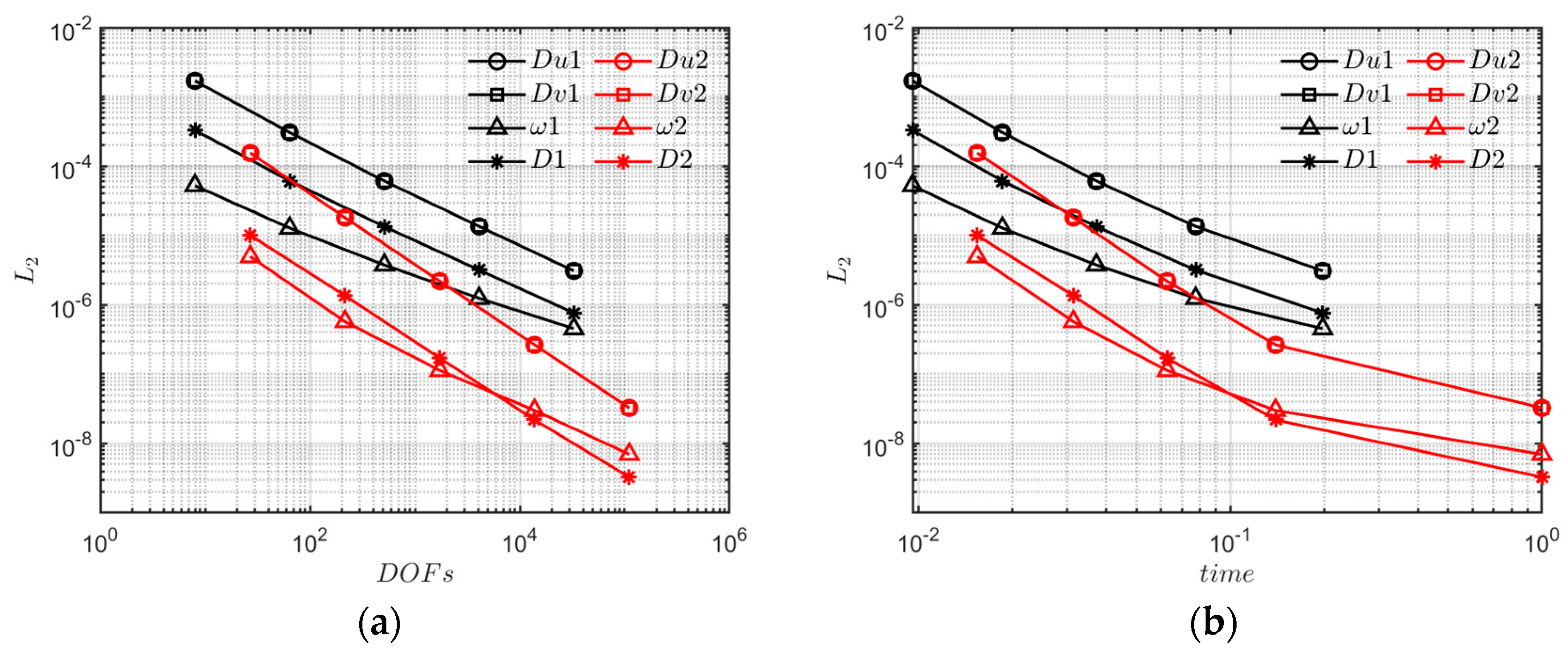
4.1. Manufactured Solution

This test is used to verify the convergence property of the developed model. As the 3D SWEs are a non-linear system, designing a nontrivial function satisfying the equations and the boundary conditions at the same time is not a trivial task. Following the philosophy presented by Salari and Knupp [39], we manually give the solution that satisfies the continuity equation and solve a Dirichlet problem for a modified system that includes a forcing term.

For this test, the Coriolis acceleration terms are not included, the horizontal eddy viscosity coefficient $K_h$ is taken as 0.1 m² s⁻¹, the vertical eddy viscosity coefficient $K_m$ is taken as 0.01 m² s⁻¹, and the analytical solution is given as follows:

$$\begin{array}{l}b\left(x,y,t\right)=-\left(2-0.005\left(x+y\right)\right),\\ \eta \left(x,y,t\right)=0.01\left(\sin \left(0.01\left(x+t\right)\right)+\sin \left(0.01\left(y+t\right)\right)\right),\\ u\left(x,y,\sigma ,t\right)=0.1{\left(D\left(1+\sigma \right)\right)}^3\sin \left(0.01\left(x+t\right)\right),\\ v\left(x,y,\sigma ,t\right)=0.1{\left(D\left(1+\sigma \right)\right)}^3\sin \left(0.01\left(x+t\right)\right).\end{array}$$

(52)

The vertical velocity at an arbitrary location is obtained through the integration of the continuity equation, Equation (11), from the bottom to the studied location. The horizontal projection of the horizontal domain is ${\Omega }_{2d}=\left[0,100\right]\times \left[0,100\right]$, and the whole simulation lasts for 86.4 s.

Tests are run with successively refined meshes. For the coarsest mesh, there is one element in the horizontal direction and one layer in the vertical direction. We refine the mesh up to four times by partitioning each quadrilateral prism into eight and compute the $L_2$ error of the numerical results against the analytical solutions as

$$L_2=\frac{1}{{\displaystyle {\sum }_e{\displaystyle {\int }_{{\Omega }_e}d\mathit{x}}}}{\left({\displaystyle {\sum }_e{\displaystyle {\int }_{{\Omega }_e}{\left(Q_e^S\left(\mathit{x}\right)-Q_e^{exact}\left(\mathit{x}\right)\right)}^{2}d\mathit{x}}}\right)}^{1/2},$$

(53)

where $Q_e^S\left(\mathbf{x}\right)$ is the numerical result and $Q_e^{exact}\left(\mathit{x}\right)$ is the analytical solution. To measure the convergence properties of the model, we further define the convergence rate (CR) as follows

$$CR={\log }_2\left(L_2^m/L_2^{m-1}\right)/{\log }_2\left(L^m/L^{m-1}\right),$$

(54)

where $L_2^m$ and $L_2^{m-1}$ are the numerical errors on two successive refined meshes and $L^m$ and $L^{m-1}$ are the characteristic lengths of the meshes, which are set to be the longest edge length of the quadrilateral prisms. Table 3 and Table 4 give the $L_2$ error for each variable and the corresponding CR for $N_h=N_v=1$ and 2, respectively. $N_e$ denotes the number of elements in the horizontal direction and $N_L$ the number of vertical layers. We note that for water depth $D$, horizontal momenta $Du$ and $Dv$ converge at the optimal rate, i.e., CR = 2 for the former case and 3 for the latter, whereas the vertical velocity $\omega$ converges at the suboptimal rate for both cases. We owe this to the fact that the vertical velocity is computed from the numerical results for $Du$, $Dv$, and their depth-averaged counterparts using the continuity Equation (42), and the CR for vertical velocity would be influenced as the horizontal momenta are not exact, as pointed out by Dawson and Aizinger [25].

Table 3. $N_h=N_v=1$, the L₂ error for each variable, and the corresponding CR.

Ne	NL	Er(D)	CR(D)	Er(Du)	CR(Du)	Er(Dv)	CR(Dv)	Er(ω)	CR(ω)
1	1	0.00033		0.00169		0.00169		$5.224\times 10^{-5}$
4	2	$6.125\times 10^{-5}$	2.42	0.00031	2.47	0.00031	2.47	$1.277\times 10^{-5}$	2.03
16	4	$1.340\times 10^{-5}$	2.19	$6.086\times 10^{-5}$	2.33	$6.086\times 10^{-5}$	2.33	$3.748\times 10^{-6}$	1.77
64	8	$3.170\times 10^{-6}$	2.08	$1.350\times 10^{-5}$	2.17	$1.350\times 10^{-5}$	2.17	$1.239\times 10^{-6}$	1.60
256	16	$7.617\times 10^{-7}$	2.06	$3.083\times 10^{-6}$	2.13	$3.083\times 10^{-6}$	2.13	$4.527\times 10^{-7}$	1.45

Table 4. $N_h=N_v=2$, the L₂ error of each variable, and the corresponding CR.

Ne	NL	Er(D)	CR(D)	Er(Du)	CR(Du)	Er(Dv)	CR(Dv)	Er(ω)	CR(ω)
1	1	$9.997\times 10^{-6}$		0.00015		0.00015		$4.95\times 10^{-6}$
4	2	$1.353\times 10^{-6}$	3.10	$1.804\times 10^{-5}$	3.10	$1.804\times 10^{-5}$	3.10	$5.71\times 10^{-7}$	3.11
16	4	$1.703\times 10^{-7}$	3.04	$2.187\times 10^{-6}$	3.04	$2.187\times 10^{-6}$	3.04	$1.13\times 10^{-7}$	2.33
64	8	$2.196\times 10^{-8}$	3.05	$2.649\times 10^{-7}$	3.05	$2.649\times 10^{-7}$	3.05	$3.00\times 10^{-8}$	1.91
256	16	$3.276\times 10^{-9}$	3.02	$3.264\times 10^{-8}$	3.02	$3.264\times 10^{-8}$	3.02	$6.99\times 10^{-9}$	2.10

Figure 2 shows the relation between the $L_2$ error and DOFs and the normalized CPU time. Figure 2a indicates that the developed model is convergent, as the $L_2$ error for each variable diminishes in both cases as the computational mesh is refined. Figure 2b indicates that we can achieve a given error tolerance with fewer DOFs on a coarser mesh when a higher approximation order is adapted. For example, when the error tolerance about water depth $D$ is taken as $1.0\times {10}^{-6}$, the normalized CPU time is about 0.033 when the approximation order is $N_h=N_v=2$, whereas it is about 0.18 when the approximation order is $N_h=N_v=1$.

Figure 2. L² error versus DOFs and normalized CPU time for water depth D, vertical velocity ω, and horizontal momenta Du and Dv at different approximation orders (N_h = N_v = 1(black), N_h = N_v = 2(red)) on a sequence of meshes. (a) L² error versus DOFs; (b) L² error versus normalized CPU time.

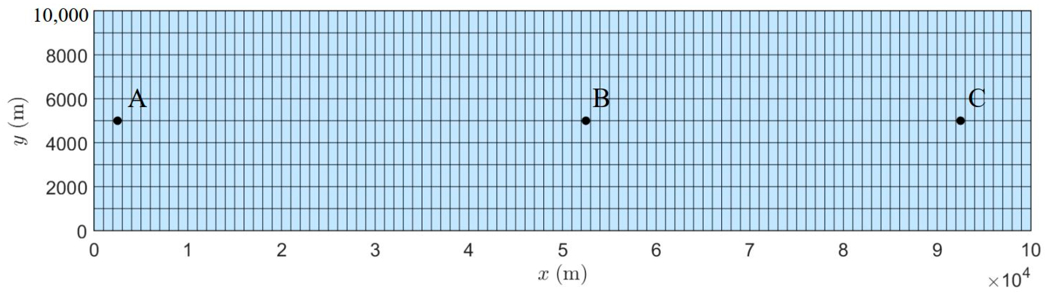
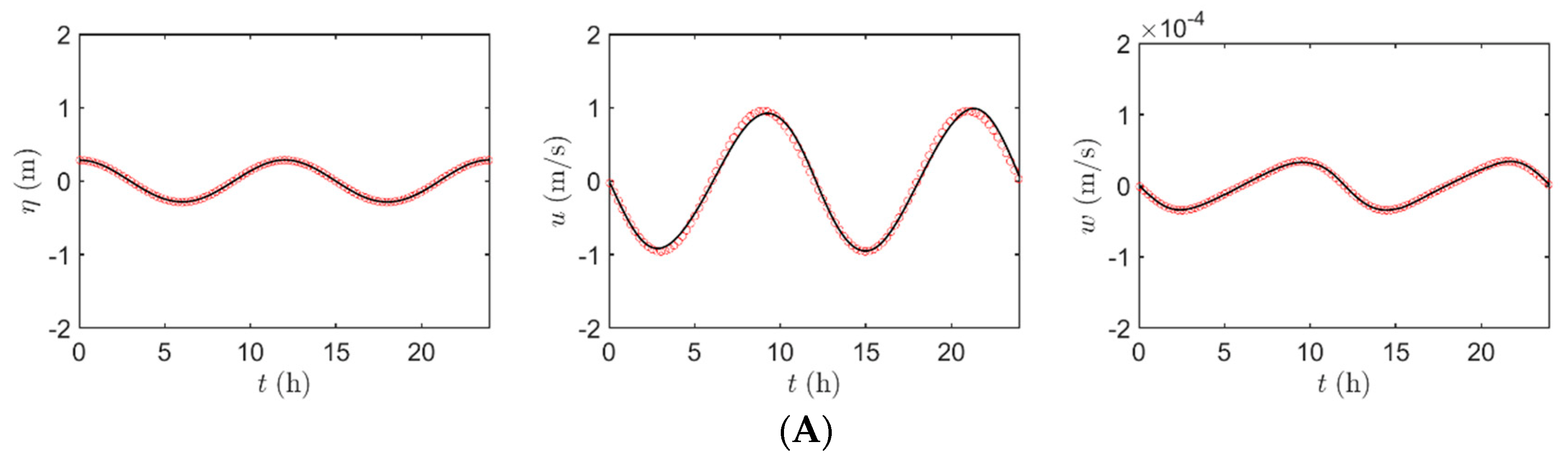
4.2. Tide Wave Propagation in a Semi-Closed Bay

This test is used to indicate the accuracy of the developed model for the simulation of both the horizontal and vertical velocity fields. Figure 3 shows the horizontal locations of Gauge points A (2500, 5000), B (52,500, 5000), and C (92,500, 5000) and a sketch of the horizontal domain. This domain is 100,000 m long and 10,000 m wide and is partitioned by a uniform quadrilateral element with a size of 1000 m in both directions. The still water depth is h = 12 m. A cosine tidal wave with amplitude A = 0.25 m and period T = 12 h is imposed at the left boundary, i.e., x = 0, whereas the other boundaries are all treated as slip walls. Both the eddy viscosity terms and the Coriolis acceleration terms are not included.

Figure 3. Location of the gauge points and sketch of the two-dimensional computational domain.

According to Neuman and Pierson [40], the analytical solution of the surface elevation $\eta$, the horizontal velocities $u$ and $v$, and the vertical velocity $w$ at a point P(x, y, z) at time $t$ are given as

$$\begin{array}{l}\eta \left(x,t\right)=A\left[\cos \left(\frac{{\omega }^{\prime }}{\sqrt{gh}}\left(L-x\right)\right)/\cos \left(\frac{{\omega }^{\prime }}{\sqrt{gh}}L\right)\right]\cos \left({\omega }^{\prime }t\right),\\ u\left(x,t\right)=-\left[\left(A\frac{\sqrt{gh}}{h}\right)/\cos \left(\frac{{\omega }^{\prime }}{\sqrt{gh}}L\right)\right]\sin \left(\frac{{\omega }^{\prime }}{\sqrt{gh}}\left(L-x\right)\right)\sin \left({\omega }^{\prime }t\right),\\ v\left(x,t\right)=0,\\ w\left(z,t\right)=-\frac{h+z}{\eta +h}A{\omega }^{\prime }\sin \left({\omega }^{\prime }t\right)\left[\cos \left(\frac{{\omega }^{\prime }}{\sqrt{gh}}\left(L-x\right)\right)/\cos \left(\frac{{\omega }^{\prime }}{\sqrt{gh}}L\right)\right]\\ -\frac{h+z}{\eta +h}\frac{A^2{\omega }^{\prime }}{h}\frac{1}{{\cos }^2\left({\omega }^{\prime }L/\sqrt{gh}\right)}\cos \left({\omega }^{\prime }t\right)\sin \left({\omega }^{\prime }t\right).\end{array}$$

(55)

where ${\omega }^{\prime }=2\pi /T$ is the frequency. For the initial condition, all the velocity components are set to zero, and the surface elevation is set according to the analytical solution. The number of vertical layers is set to 12, and we run this simulation for 24 h.

Figure 4 gives the comparison between the numerical result and the analytical solution for surface elevation $\eta$, horizontal velocity $u$, and vertical velocity $w$ at Gauges A, B, and C, and the vertical coordinate for the three Gauges is $z$= −2.5 m. It can be seen that the numerical solution is generally in good agreement with the analytical solution, indicating that the three-dimensional model developed in this study has good accuracy in the simulation of water level and velocity.

Figure 4. Comparison between the numerical result (black line) and the analytical solution (red circle) for surface elevation $\eta$, horizontal velocity $u$, and vertical velocity $w$ at Gauges (A–C).

4.3. Wind-Induced Water Circulation

In this test, the wind-driven circulation in a rectangular closed basin is simulated. Following Liu et al. [41], we run this case to test the accuracy of the proposed numerical model in predicting the vertical stratified circulation.

With a homogeneous Dirichlet boundary condition adapted at the bottom boundary, Koutitas et al. [42] derived the analytical solution of the horizontal velocity in the center of the basin as

$$u\left(\sigma \right)=\frac{{\tau }_{sx}\left(\sigma +1\right)h\left(3\sigma +1\right)}{4K_v{\rho }_0}. \sigma \in \left[-1,0\right]$$

(56)

where $h$ is the still water depth of the basin. Likewise, Huang [43] also derived that when the Neumann boundary condition is adapted, the result reads

$$\begin{array}{l}u\left(\sigma \right)=\frac{1}{6K_v}g\frac{\partial \eta }{\partial x}{h}^2\left(3{\sigma }^2-1\right)+\frac{{\tau }_{sx}h}{2{\rho }_0{K}_v}\left(2\sigma +1\right), \sigma \in \left[-1,0\right]\\ \frac{\partial \eta }{\partial x}=\frac{3}{2}\frac{{\tau }_{sx}}{{\rho }_{0}gh}\frac{2K_v+C_f\left|u_c\right|h}{3K_v+C_f\left|u_c\right|h},\end{array}$$

(57)

where $\left|u_c\right|$ is the velocity magnitude at the center of the bottommost element, and $C_f\left|u_c\right|=0.005 m/s$ in this study. In this part, these two situations are simulated.

This case is set as follows: the basin is 2000 m long and 800 m wide, $h=10 \mathrm{m}$, and ${\tau }_{sx}=1.5 Pa$. The Coriolis acceleration and horizontal eddy viscosity terms are ignored, and the vertical eddy viscosity coefficient $K_m$ is set to be 0.001 m² s⁻¹; the whole simulation lasts for 3600 s.

Figure 5a,b shows the comparison between the numerical results and the analytical solution for the vertical distribution of horizontal velocity at the center of the basin. The comparison indicates that the numerical results match well with the analytical solution for both cases.

Figure 5. Comparison between the numerical results and the analytical solution for the vertical distribution of horizontal velocity at the center of the basin. (a) Homogeneous Dirichlet boundary condition; (b) Neumann boundary condition.

We also run the simulations with different numbers of vertical layers ($N_L$). To quantitatively measure the difference between different simulations, we define the root mean square error (RMSE) as

$$\mathrm{RMSE}=\sqrt{\frac{{\displaystyle \sum _{j=1}^{N_T}{\left(u_{a,j}-u_j\right)}^2}}{N_T}},$$

(58)

where $N_T$ is the number of simulated results, $u_j$ is the numerical result at point $j$, and $u_{a,j}$ is the analytical solution at the same point. Table 5 gives the RMSE for different simulations. We find that the more vertical layers there are, the better the result will be for each case.

Table 5. RMSE for simulations with different vertical layers and different boundary conditions.

NL	5	10	15	20
	Homogeneous Dirichlet boundary condition
RMSE	0.0107	0.0051	0.0041	0.0037
	Neumann boundary condition
RMSE	0.0219	0.0138	0.0114	0.0103

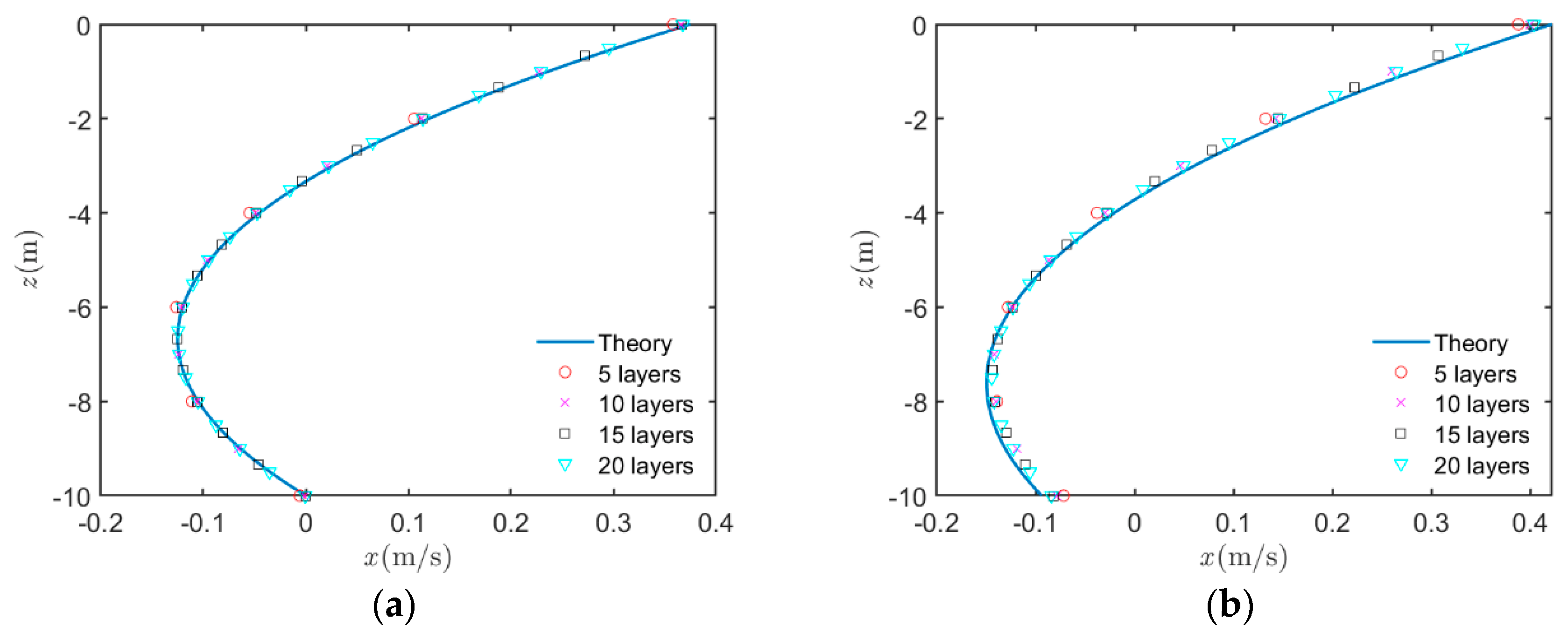
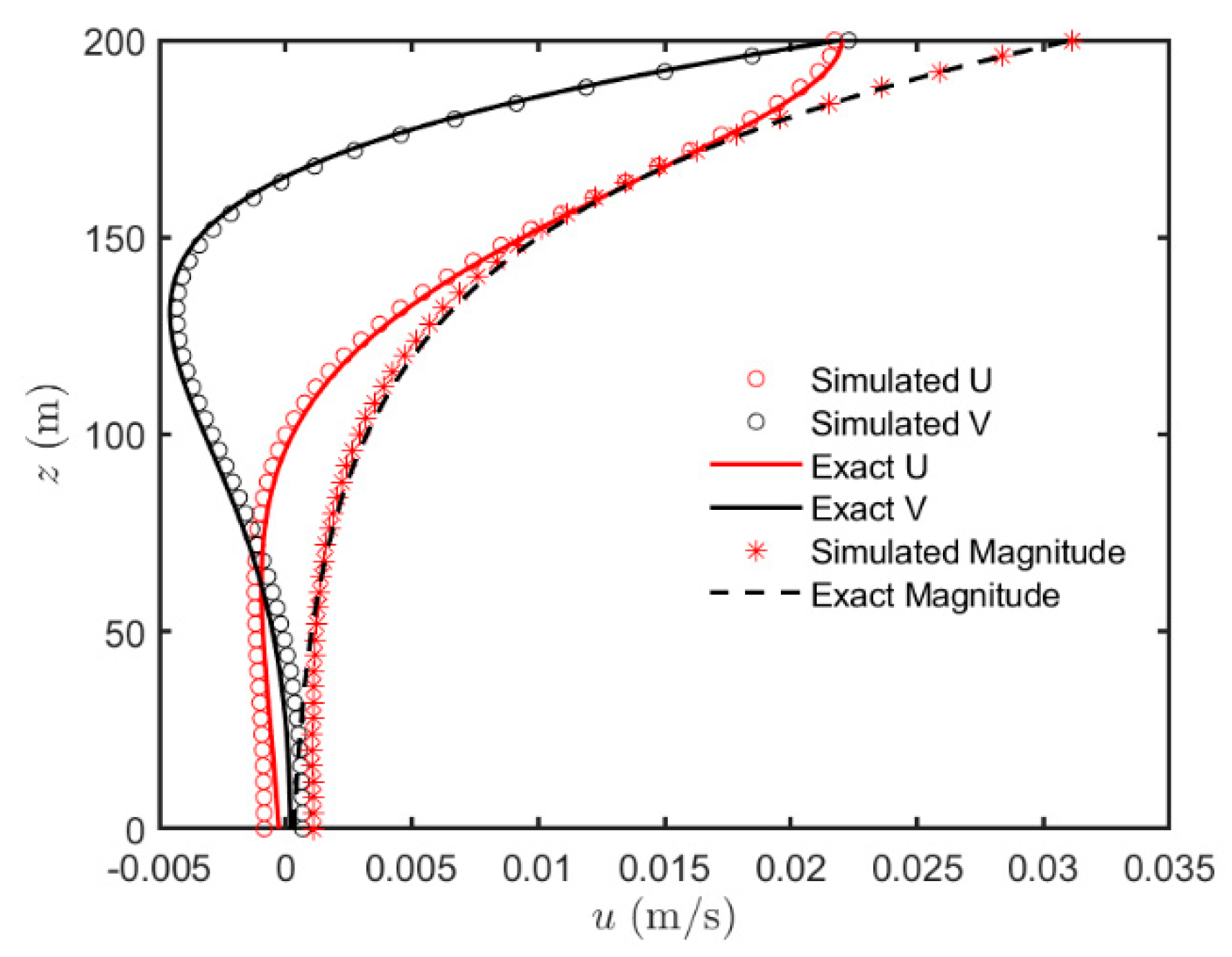
4.4. Generation of the Ekman Profile

Following Trahan et al. [44], we run this test to check whether the developed model can generate the Ekman layer, where the Coriolis acceleration terms, the pressure gradient, and the turbulent drag are in balance. The analytic solution for the Ekman velocity profile was developed by Ekman [45] and is expressed as

$$\begin{array}{l}u=u_0{e}^{\left(-z/D_f\right)}\cos \left(\frac{\pi }{4}-\frac{z}{D_f}\right),\\ v=v_0{e}^{\left(-z/D_f\right)}\sin \left(\frac{\pi }{4}-\frac{z}{D_f}\right),\\ v_0=\frac{{\tau }_{sx}}{\rho {\left(K_{v}f\right)}^{0.5}},\\ D_f={\left(\frac{2K_v}{f}\right)}^{0.5},\\ f=2\varpi \sin \theta .\end{array}$$

(59)

where $D_f$ is the folding depth, $K_v=0.1$ m²/s, ${\tau }_{sx}=0.1$ Pa, and $\theta$ is the geophysical latitude (${45}^{°}$). Theoretically, the flow direction at the surface would rotate counterclockwise 45 degrees to that of the wind stress.

The computational domain is 40,000 km long and 40,000 km wide and is partitioned by a uniform quadrilateral element with a size of 2000 km in both directions. A constant depth of 200 m is set, and 50 vertical layers are used. The bottom drag coefficient $C_f$ is set to 0.0025. We run this simulation for 200 days. Figure 6 gives the comparison of the analytic solution and the computed Ekman profile. The numerical results accurately match the analytic solution and individual velocity components with an average error of less than 0.001 m/s.

Figure 6. Comparison between the numerical results and the analytical solution for individual velocity components and velocity magnitude for the Ekman profile.

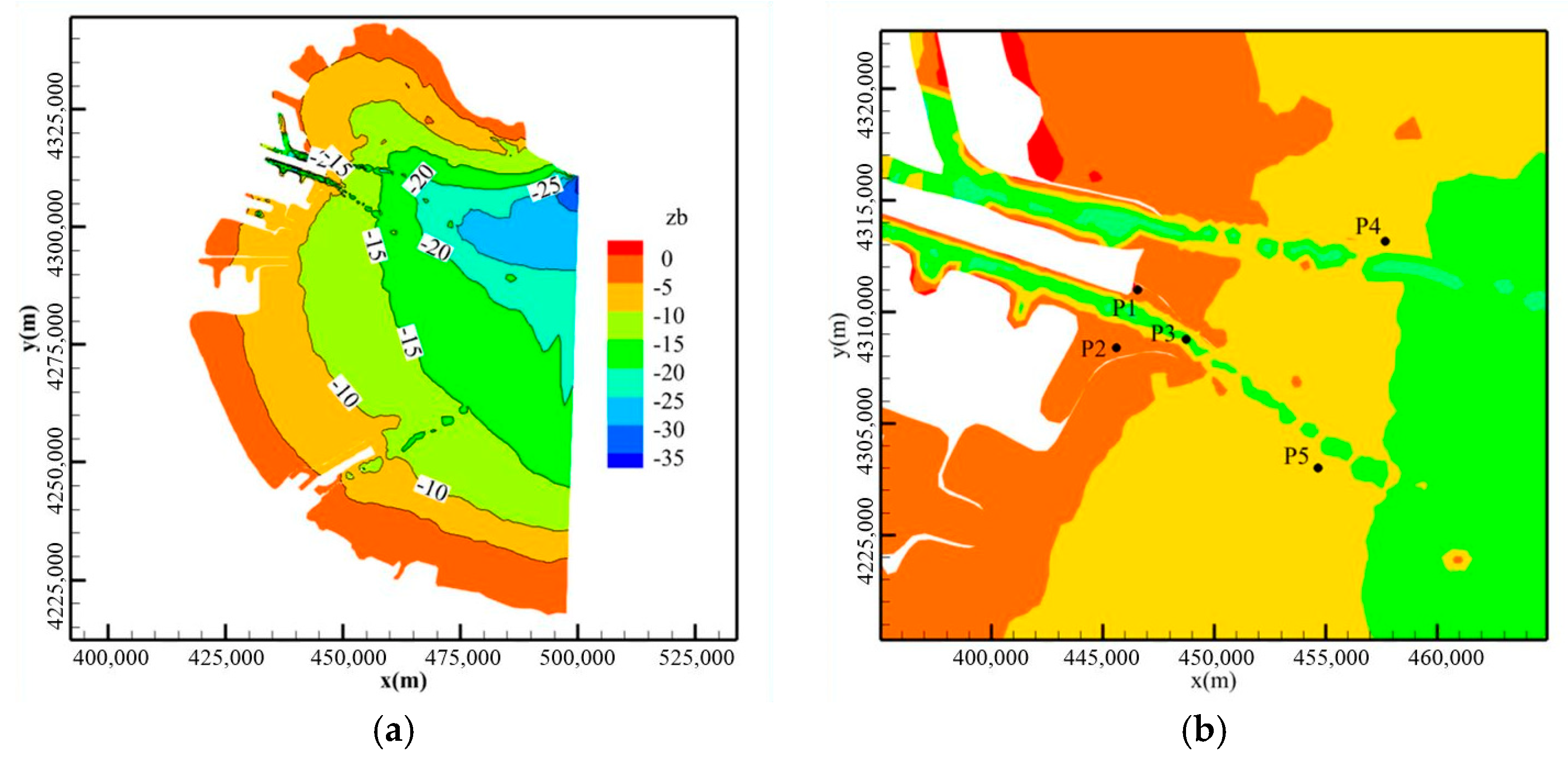
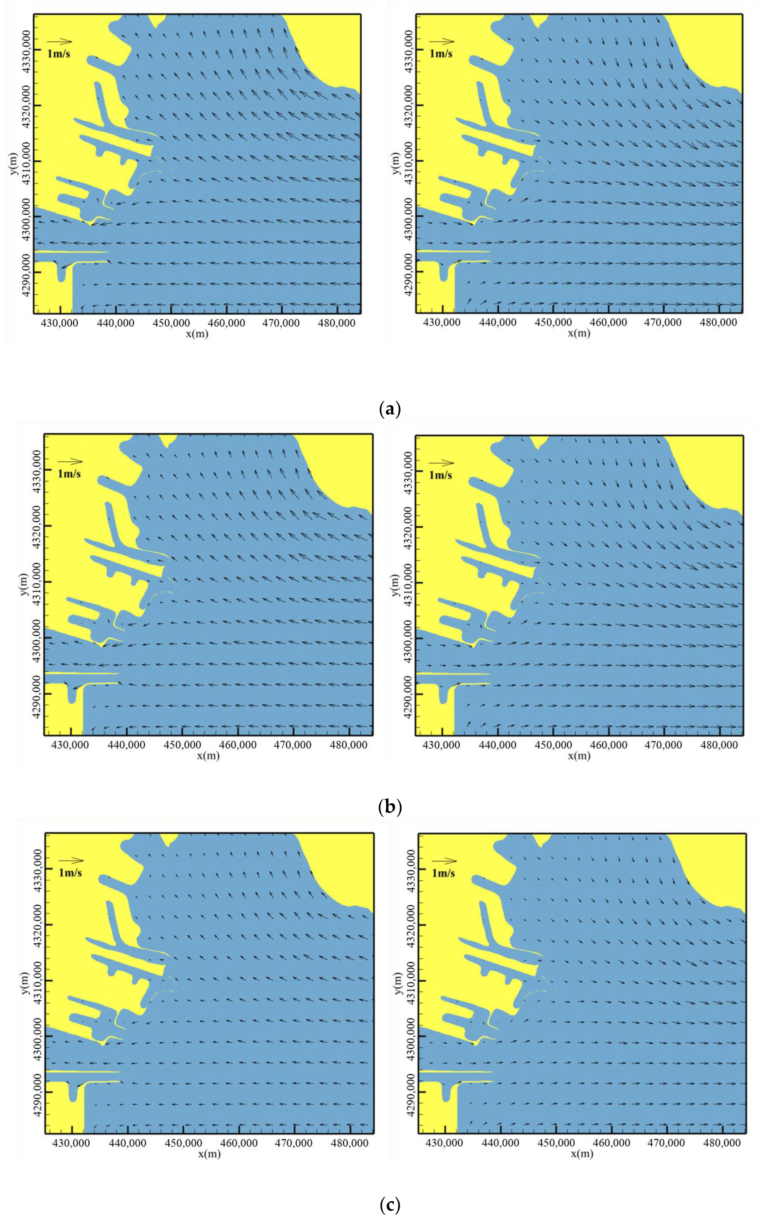
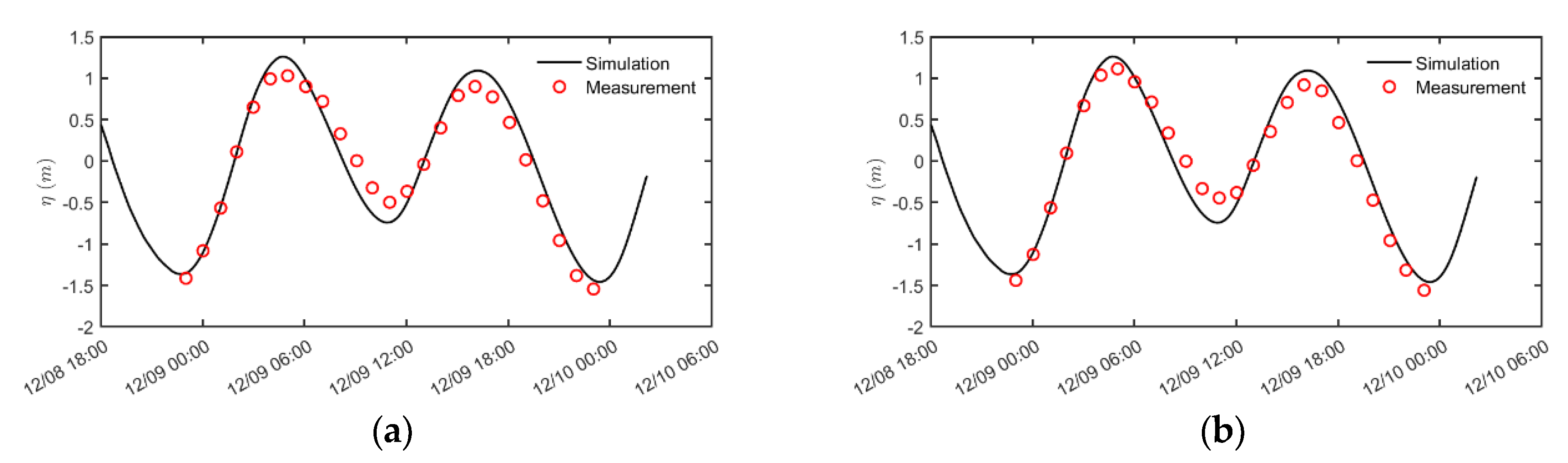
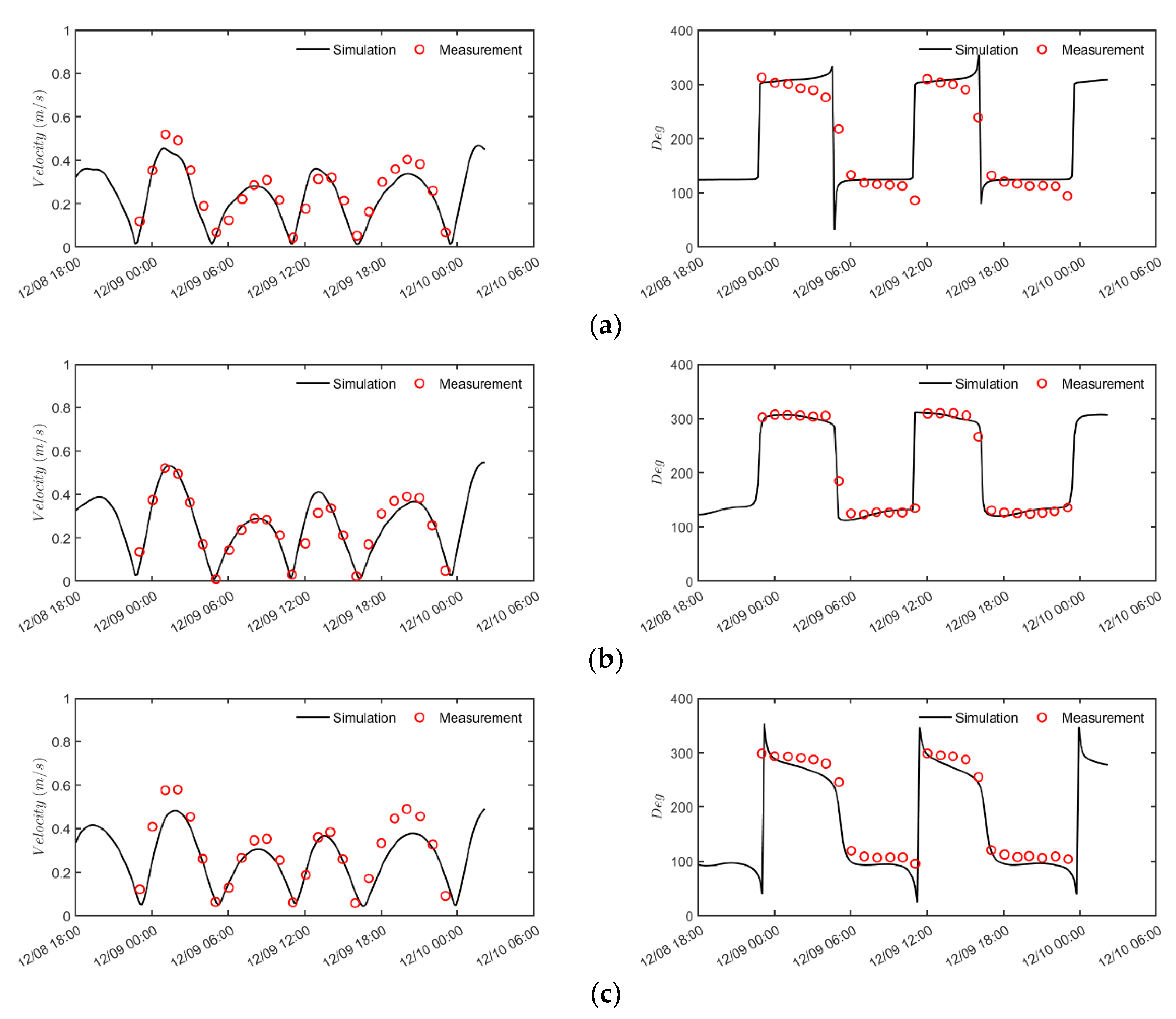
4.5. Tidal Flow in Bohai Bay

For the last case, we simulate tidal flow in the western region of Bohai Bay to test the ability of the developed model for the simulation of actual tidal wave motion problems. The Bohai Bay is one of the three major bays of the Bohai Sea in China. It is located in the west of the Bohai Sea and connected with Hebei and Shandong Province and Tianjin City. It’s a typical semi-closed sea area. The average tidal range in Bohai Bay is 2.5 m, and its tidal current is irregularly semi-diurnal. In recent years, a lot of port and reclamation projects in Bohai Bay have been carried out, which has led to a large number of large-scale engineering structures. The accurate simulation of the tidal current field is of great significance for the convection–diffusion process of temperature, salt, pollutants, etc., as well as the sediment transport in Bohai Bay.

The domain geometry for this case is shown in Figure 7a; the still water depth ranges from 38 m at the east open boundary to 2 m at the coast. There are five measuring gauges in the computational domain, and the distribution of these points is shown in Figure 7b. The computational domain is partitioned by 14,627 triangle grids, and the edge length of the finite element mesh ranges from 2 km to 100 m. Five equidistant layers are used in the vertical direction. Wetting/drying is not accounted in the present study.

Figure 7. Computational domain geometry for tidal flow in the west region of Bohai Bay. (a) Computational domain geometry; (b) Gauge points.

The tidal elevations at the east open boundaries were provided by Chinatide [46], which is a tidal forecast system through nine harmonic constants of Q₁, P₁, O₁, K₁, N₂, M₂, S₂, K₂, and Sa. The Coriolis parameter was taken as $9.1557\times {10}^{-5}{\mathrm{s}}^{-1}$, and the horizontal eddy viscosity coefficient was set to 70 m² s⁻¹. The vertical eddy viscosity coefficient was modelled using the $k-ϵ$ turbulence closures provided by GOTM [47], and the coupling between GOTM and the hydrodynamic model is established following the same philosophy presented by Tuomas et al. [32]. The bottom roughness length is set as 0.1 mm. Field measurements from 12/08/2018 to 12/09/2018 are used to verify the developed model.

Figure 8 shows the flow field at the surface and the middle and bottom layers at the time of flood tide (left) and ebb tide (right), respectively. As we can see, there is little difference between the velocity fields of the surface and the middle layers. Because of the bottom friction, the velocity of the bottom layer is smaller than that of the surface and the middle layers, which is about 60% of the magnitude of the latter two. The results of the three-dimensional velocity field show that the model can reflect the three-dimensional characteristics of tidal flow.

Figure 8. Flow field at different levels at the flood tide (left column) and the ebb tide (right column). (a) surface ($\mathsf{\sigma }=0$); (b) middle ($\mathsf{\sigma }=-0.5$); (c) bottom ($\mathsf{\sigma }=-1.0$).

Figure 9 shows the comparison between the simulated surfaced elevation and the field measurements at Gauges P1 and P2. The simulated data are quantitatively very close to the field measurements, and the tidal phasing is virtually identical. The left column of Figure 10 gives the comparison between the simulated velocity and the field measurements at gauges P3, P4, and P5. Small discrepancies exist between the simulated velocity and the field measurements. This is especially the case for P5, where the maximum simulated velocity is about 15% smaller than that of the field measurements. It can be attributed to that the computational mesh used in this simulation is relatively coarse, and the wetting/drying is not considered. Although differences exist, the simulated data are in phase with the field measurements as the comparison between the simulated flow direction and the field measurements shows in the right column of Figure 10. Generally, the developed hydrodynamic model can be used for the simulation of tidal wave motion in realistic situations.

Figure 9. Comparison between the numerical results and the measured surface elevation at Gauges P1 and P2 for the Bohai Bay case. (a) P1; (b) P2.

Figure 10. Comparison between the simulated results and the measured data for velocity (left column) and flow direction (right column) at Gauges P3, P4, and P5 for the Bohai Bay case. (a) P3; (b) P4; (c) P5.

5. Conclusions

In this study, a three-dimensional hydrodynamic model based on the Discontinuous Galerkin method is developed. The $\sigma$-coordinate system is used in the vertical direction to circumvent the mismatch of lateral faces due to the discontinuous nature of the solution between different elements. Non-linear advective terms are included, and the model is marched in time with the implicit-explicit Runge–Kutta method. The vertical eddy viscosity and the Coriolis acceleration terms are discretized with the symmetric interior penalty discontinuous Galerkin method and are treated implicitly, while others are treated explicitly.

The developed model is validated with a series of numerical tests. The case with the manufactured solution indicates that the model is convergent, and the $L_2$ error about the variables diminishes as we increase the approximation order or refine the computational mesh. Calculating the CR indicates that water depth $D$ and horizontal momenta $Du$ and $Dv$ can all converge at the optimal order, whereas the vertical velocity converges in a suboptimal order. This case also indicates that we can obtain a better numerical result on a computational mesh with fewer DOFs when a higher approximation is adapted. Cases of tide-induced three-dimensional flow in a semi-closed bay, wind-induced water circulation, and the generation of the Ekman profile indicate that the developed model can well simulate the velocity field in both horizontal and vertical directions, can reasonably simulate the vertical stratified circulation, and can simulate water motion under the combined effect of wind stress and Coriolis acceleration terms. For the Bohai Bay case, the simulated surface elevation, velocity, and flow direction match reasonably well with the field measurements, indicating the model can be used for the simulation of tidal wave motion in realistic situations.

More applications of the developed model and development of the wetting/drying treatment and the baroclinic model will be presented in forthcoming work.

References

- Lee, J.; Lee, J.; Yun, S.-L.; Kim, S.-K. Three-Dimensional Unstructured Grid Finite-Volume Model for Coastal and Estuarine Circulation and Its Application. Water 2020, 12, 2752. [Google Scholar] [CrossRef]
- Blaise, S.; Comblen, R.; Legat, V.; Remacle, J.-F.; Deleersnijder, E.; Lambrechts, J. A discontinuous finite element baroclinic marine model on unstructured prismatic meshes. Ocean. Dyn. 2010, 60, 1371–1393. [Google Scholar] [CrossRef]
- Li, L.; Zhang, Q. Development of an efficient wetting and drying treatment for shallow-water modeling using the quadrature-free Runge-Kutta discontinuous Galerkin method. Int. J. Numer. Methods Fluids 2021, 93, 314–338. [Google Scholar] [CrossRef]
- Ran, G.; Zhang, Q.; Li, L. A depth-integrated non-hydrostatic model for nearshore wave modelling based on the discontinuous Galerkin method. Ocean. Eng. 2021, 232, 108661. [Google Scholar] [CrossRef]
- Di Pietro, D.A.; Marche, F. Weighted interior penalty discretization of fully nonlinear and weakly dispersive free surface shallow water flows. J. Comput. Phys. 2018, 355, 285–309. [Google Scholar] [CrossRef]
- Shchepetkin, A.F.; McWilliams, J.C. The regional oceanic modeling system (ROMS): A split-explicit, free-surface, topography-following-coordinate oceanic model. Ocean. Model. 2005, 9, 347–404. [Google Scholar] [CrossRef]
- Mellor, G. Users Guide for a Three-Dimensional, Primitive Equation, Numerical Ocean Model; Princeton University: Princeton, NJ, USA, 2004. [Google Scholar]
- Griffies, S.M. Elements of the Modular Ocean Model (MOM); GFDL Ocean Group Technical Report; NOAA: Princeton, NJ, USA, 2012. [Google Scholar]
- Burchard, H.; Bolding, K. GETM: A General Estuarine Transport Model. Scientific Documentation; European Commission Technical Report EUR 20253 EN; European Commission: Brussels, Belgium, 2002; p. 157. [Google Scholar]
- Casulli, V.; Cheng, R.T. Semi-implicit finite difference methods for three-dimensional shallow water flow. Int. J. Numer. Methods Fluids 1992, 15, 629–648. [Google Scholar] [CrossRef]
- Deltares Systems. User Manual of Delft3D-FLOW—Simulation of Multi-Dimensional Hydrodynamic Flows and Transport Phenomena, Including Sediments; Report of Delft Hydraulics; Deltares: Delft, The Netherlands, 2003; p. 497. [Google Scholar]
- Hamrick, J.; Wu, T. Computational Design and Optimization of the EFDC/HEM3D Surface Water Hydrodynamic and Eutrophication. In Next Generation Environmental Models and Computational Methods; Society for Industrial and Applied Mathematics: Philadelphia, PA, USA, 1997; pp. 143–161. [Google Scholar]
- Blumberg, A.F.; Mellor, G.L. A Description of a Three-Dimensional Coastal Ocean Circulation Model; AGU: Washington, DC, USA, 1987; pp. 1–16. [Google Scholar]
- Luyten, P.J.; Jones, J.E.; Proctor, R. A numerical study of the long-and short-term temperature variability and thermal circulation in the North Sea. J. Phys. Oceanogr. 2003, 33, 37–56. [Google Scholar] [CrossRef]
- Alistair, A.; Jean-Michel, C.; Stephanie, D.; Constantinos, E.; David, F.; Gael, F.; Baylor, F.-K.; Patrick, H.; Chris, H.; Ed, H. Mitgcm User Manual; MIT: Cambridge, MA, USA, 2018. [Google Scholar]
- Martins, F.; Leitão, P.; Silva, A.; Neves, R. 3D modelling in the Sado estuary using a new generic vertical discretization approach. Oceanol. Acta 2001, 24, 51–62. [Google Scholar] [CrossRef]
- Chen, C.; Beardsley, R.; Cowles, G.; Qi, J.; Lai, Z.; Gao, G.; Stuebe, D.; Xu, Q.; Xue, P.; Ge, J. An Unstructured-Grid, Finite-Volume Community Ocean Model: FVCOM User Manual; SMAST/UMASSD Technical Report-13-0701; MIT: Cambridge, MA, USA, 2012; p. 404. [Google Scholar]
- Casulli, V.; Walters, R.A. An unstructured grid, three-dimensional model based on the shallow water equations. Int. J. Numer. Methods Fluids 2000, 32, 331–348. [Google Scholar] [CrossRef]
- Nan, Z.; Sheng, J.; Congfang, A.; Weiye, D. An integrated water-conveyance system based on Web GIS. J. Hydroinform. 2018, 20, 668–686. [Google Scholar] [CrossRef]
- Wang, Q. The Finite Element Ocean Model and Its Aspect of Vertical Discretization. Ph.D. Thesis, Universität Bremen, Bremen, Germany, 2007. [Google Scholar]
- Zhang, Y.; Baptista, A.M. SELFE: A semi-implicit Eulerian–Lagrangian finite-element model for cross-scale ocean circulation. Ocean. Model. 2008, 21, 71–96. [Google Scholar] [CrossRef]
- Luettich, R.A.; Westerink, J.J.; Scheffner, N.W. ADCIRC: An Advanced Three-Dimensional Circulation Model for Shelves, Coasts, and Estuaries. Report 1, Theory and methodology of ADCIRC-2DD1 and ADCIRC-3DL; Department of the Army, US Army Corps of Engineers Waterways Experiment Station, Coastal Engineering Research Center: Vicksburg, MS, USA, 1992. [Google Scholar]
- Zhang, Y.J.; Ye, F.; Stanev, E.V.; Grashorn, S. Seamless cross-scale modeling with SCHISM. Ocean. Model. 2016, 102, 64–81. [Google Scholar] [CrossRef]
- Hervouet, J.-M. Hydrodynamics of Free Surface Flows: Modelling with the Finite Element Method; John Wiley & Sons: Hoboken, NJ, USA, 2007. [Google Scholar]
- Dawson, C.; Aizinger, V. A discontinuous Galerkin method for three-dimensional shallow water equations. J. Sci. Comput. 2005, 22, 245–267. [Google Scholar] [CrossRef]
- Aizinger, V.; Dawson, C. The local discontinuous Galerkin method for three-dimensional shallow water flow. Comput. Methods Appl. Mech. Eng. 2007, 196, 734–746. [Google Scholar] [CrossRef]
- Aizinger, V.; Proft, J.; Dawson, C.; Pothina, D.; Negusse, S. A three-dimensional discontinuous Galerkin model applied to the baroclinic simulation of Corpus Christi Bay. Ocean. Dyn. 2013, 63, 89–113. [Google Scholar] [CrossRef]
- Blaise, S. Development of a Finite Element Marine Model. Ph.D. Thesis, UCL-Université Catholique de Louvain, Ottignies-Louvain-la-Neuve, Belgium, 2009. [Google Scholar]
- Comblen, R. Discontinuous Finite-Element Methods for Two-and Three-Dimensional Marine Flows. Ph.D. Thesis, UCL-Université Catholique de Louvain, Ottignies-Louvain-la-Neuve, Belgium, 2010. [Google Scholar]
- Gandham, R. High Performance High-Order Numerical Methods: Applications in Ocean Modeling. Ph.D. Thesis, Rice University, Houston, TX, USA, 2015. [Google Scholar]
- Conroy, C.J.; Kubatko, E.J. Hp discontinuous Galerkin methods for the vertical extent of the water column in coastal settings part I: Barotropic forcing. J. Comput. Phys. 2016, 305, 1147–1171. [Google Scholar] [CrossRef]
- Kärnä, T.; Legat, V.; Deleersnijder, E.; Burchard, H. Coupling of a discontinuous Galerkin finite element marine model with a finite difference turbulence closure model. Ocean. Model. 2012, 47, 55–64. [Google Scholar] [CrossRef]
- Phillips, N.A. A coordinate system having some special advantages for numerical forecasting. J. Atmos. Sci. 1957, 14, 184–195. [Google Scholar] [CrossRef]
- Toro, E.F. Shock-Capturing Methods for Free-Surface Shallow Flows; John Wiley and Sons: Hoboken, NJ, USA, 2001. [Google Scholar]
- Hesthaven, J.S.; Warburton, T. Nodal Discontinuous Galerkin Methods: Algorithms, Analysis, and Applications; Springer Science & Business Media: Berlin/Heidelberg, Germany, 2007. [Google Scholar]
- Cockburn, B.; Shu, C.-W. The local discontinuous Galerkin method for time-dependent convection-diffusion systems. SIAM J. Numer. Anal. 1998, 35, 2440–2463. [Google Scholar] [CrossRef]
- Di Pietro, D.A.; Ern, A. Mathematical Aspects of Discontinuous Galerkin Methods; Springer Science & Business Media: Berlin/Heidelberg, Germany, 2011; Volume 69. [Google Scholar]
- Ascher, U.M.; Ruuth, S.J.; Spiteri, R.J. Implicit-explicit Runge-Kutta methods for time-dependent partial differential equations. Appl. Numer. Math. 1997, 25, 151–167. [Google Scholar] [CrossRef]
- Salari, K.; Knupp, P. Code Verification by the Method of Manufactured Solutions; SAND2000-1444; Sandia National Laboratories: Albuquerque, NM, USA, 2000. [Google Scholar]
- Neumann, G.; Pierson, W.J., Jr. Principles of Physical Oceanography; Prentice-Hall: Englewood Cliffs, NJ, USA, 1966. [Google Scholar]
- Liu, X.; Mohammadian, A.; Sedano, J.Á.I.; Kurganov, A. Three-dimensional shallow water system: A relaxation approach. J. Comput. Phys. 2017, 333, 160–179. [Google Scholar] [CrossRef]
- Koutitas, C.; O’Connor, B. Modeling three-dimensional wind-induced flows. J. Hydraul. Div. ASCE 1980, 106, 1843–1865. [Google Scholar] [CrossRef]
- Huang, W. Three Dimensional Numerical Modeling Of Circulation And Water Quality Induced By Combined Sewage Overflow Discharges. Ph.D. Thesis, Department of Ocean Engineering, University of Rhode Island, Kingston, RI, USA, 1993. [Google Scholar]
- Trahan, C.; Savant, G.; Berger, R.; Farthing, M.; McAlpin, T.; Pettey, L.; Choudhary, G.; Dawson, C.N. Formulation and application of the adaptive hydraulics three-dimensional shallow water and transport models. J. Comput. Phys. 2018, 374, 47–90. [Google Scholar] [CrossRef]
- Price, J.F.; Weller, R.A.; Schudlich, R.R. Wind-driven ocean currents and Ekman transport. Science 1987, 238, 1534–1538. [Google Scholar] [CrossRef]
- Li, M.; Zheng, J. Introduction to Chinatide software for tide prediction in China seas. J. Waterw. Harb. 2007, 28, 65–68. (In Chinese) [Google Scholar]
- Burchard, H.; Bolding, K.; Villarreal, M.R. GOTM, a General Ocean Turbulence Model: Theory, Implementation and Test Cases; Technical Report EUR 18745 EN; European Commission: Brussels, Belgium, 1999.
Disclaimer/Publisher’s Note: The statements, opinions and data contained in all publications are solely those of the individual author(s) and contributor(s) and not of MDPI and/or the editor(s). MDPI and/or the editor(s) disclaim responsibility for any injury to people or property resulting from any ideas, methods, instructions or products referred to in the content. |
© 2022 by the authors. Licensee MDPI, Basel, Switzerland. This article is an open access article distributed under the terms and conditions of the Creative Commons Attribution (CC BY) license (https://creativecommons.org/licenses/by/4.0/).