Article

A Quasi-Single-Phase Model for Debris Flows Incorporating Non-Newtonian Fluid Behavior

1
College of Civil Engineering, Zhejiang University of Technology, Hangzhou 310000, China
2
Planning and Development Research Institute, POWERCHINA Huadong Engineering Corporation Limited, Hangzhou 310000, China
*
Author to whom correspondence should be addressed.
Water 2022, 14(9), 1369; https://doi.org/10.3390/w14091369
Submission received: 22 March 2022 / Revised: 15 April 2022 / Accepted: 20 April 2022 / Published: 22 April 2022
(This article belongs to the Special Issue Numerical Modelling of Single and Multi-Phase Flow)

Abstract

:
Debris-flow modeling is a great challenge due to its complex physical mechanism that remains poorly understood. The present research incorporates the effect of rheological features of the non-Newtonian fluid into the complete quasi-single-phase mixture model, which explicitly accommodates the interactions between flow, non-uniform sediment transport, and bed evolution. The effect of rheological features is estimated by Hersch–Bulkley–Papanastasiou model that can be simplified to Bingham or Newtonian models with specific coefficients. The governing equations are solved by a fully conservative numerical algorithm, using an explicit finite volume discretization with well-balanced slope-limited centered scheme combined with an implicit discretization method. One set of large-scaled U.S. Geological Survey debris-flow experiments is applied to investigate the influence of the non-Newtonian fluid on debris-flow modeling. It is found that the present model closed by Hersch–Bulkley–Papanastasiou model performs better than the models without considering effect of rheological features, which may facilitate the development of quasi-single-phase mixture modeling for debris flows.

1. Introduction

Debris flow, composed of highly concentrated mixtures of sediments and water [1], is extremely destructive and represents an enormous threat to people’s life and property, public infrastructure, and ecological environment throughout their trajectories [2]. It is regarded as a physical process between landslide and flood flow. Hence, besides the characteristics of multiphase, fragmentation, flow, and yield, debris flow is also multi-scale. The shape of the solid particles that constitute debris flow is extremely irregular, and the scale spans several orders of magnitude, ranging from clay, silt, fine sand, and gravel to boulders with diameter of several meters [3]. The dynamic process of debris flow presents a series of complex physical phenomena, composed of triggering, movement, and accumulation. It is difficult to observe the whole process in the field, and therefore, numerical simulation are always carried out to study the evolution of debris flow.
The numerical dynamic model of debris flow can be divided into continuous medium model, discrete medium model, and mixed medium model [4]. The continuous medium model is generally established by fluid researchers, while the discrete medium model is usually used by geotechnical researchers. Among these two models is the mixed medium model, where the continuity of fluid and the dispersion of particles are considered. The continuous medium can be divided into quasi-single-phase model [5,6,7] and multiphase model [8,9,10,11,12]. The former is characterized by a single momentum equation for water–sediment mixture flow based on the assumption of the same velocity of fluid and solid phases, while the latter features the separate momentum equation for each phase, considering the velocity differences among phases. The two-phase model is promising for its more complete physical process to reveal the relative motions and interactions between the fluid and solid phases [11,12]. However, the high computing costs and the demand for extra closure relationships make it hard to be applied to large-scale field. In contrast, the quasi-single-phase model is more practical and has seen wide application for its much higher computation speed. However, the existing quasi-single-phase models used in engineering are often simplified. For example, some models are decoupled [13,14]; some are based on the sediment capacity assumption [15,16]; and some are restricted to uniform sediment transport cases and generally ignore the effects of debris flows fluctuations [5,17], which may not be generally justified from physical perspectives.
Meanwhile, rarely do models involve the rheological features of debris flows into a relatively complete single-phase model. However, it is known that debris flows in field cases often involve poorly sorted, heterogeneous particles in a non-Newtonian way rather than the ideal Newtonian liquid [18]. Hence, a rheological relation is warranted for numerical simulation to describe the non-Newtonian behavior of debris flow. The last several decades have witnessed the great efforts made by researchers to conduct their investigations on this field, for example, the Bingham model [19,20], Cross model [21,22], Herschel–Bulkley (HB) model [23], Herschel–Bulkley–Papanastasiou (HBP) model [24,25] and other non-Newtonian models. Among them, the Bingham model is widely used in debris-flow simulation, but the effective viscosity in the Bingham model will be infinite when the shearing rate approaches zero, leading to the divergence in the numerical simulation. Meanwhile, the Bingham model or the general Cross model in debris-flow simulations is the linear constitutive law between the shear stress tensor and the strain rate tensor under high strain rate [25]. Since many studies [26,27,28] have observed nonlinear behavior, particularly the shear thinning and shear thickening phenomenon in debris flow, the HB model is proposed and considered suitable to describe the nonlinear features of debris-flow [29]. However, the problem of numerical divergence still remains in the HB model, and Papanastasiou (1987) [24] introduced an improved version of the HB model (i.e., HBP model) to solve this problem. Here, a quasi-single-phase mixture model combined with HBP model is proposed to reveal the effect of rheological features of the non-Newtonian fluid for debris flows. The model is solved by a fully conservative numerical algorithm and then applied to the simulation of a U.S. Geological Survey debris-flow experiment.

2. Mathematical Model

The effect of rheological features of non-Newtonian fluid is incorporated into the present debris-flow model, which is an extension of the quasi-single-phase model by Xia et al. (2018) [7]. For one-dimensional debris flows over an inclined erodible bed composed of sediment with N size classes (dk denotes the diameter of the kth size sediment, and k = 1, 2, …, N), the complete depth-averaged, one-dimensional governing equations can be written as follows:
ρ m h t + ρ m h U x = ρ 0 z b t
( ρ m h U x ) t + x ( ρ m h U x 2 + 1 2 ρ g z h 2 ) = ρ m h g x ρ g z h z b x τ b + τ a d d + h ( T R + T μ ) x
h c k t + h U c k x = E k D k
z b t = E D 1 p
δ f a k t + f I k ξ t = ( D k E k ) 1 p
where t = time; x = streamwise coordinate parallel to bed slope with the angle θ ; h = debris-flow depth; U = depth-averaged mixture flow velocity in x direction; z b = bed elevation; c k = depth-averaged size-specific volumetric sediment concentration and C = c k = total volumetric sediment concentration; g = gravitational acceleration and g z = g cos θ , g x = g sin θ ; τ b = bed shear stress; p = bed sediment porosity; ρ f , ρ s = densities of fluid and solid phases, respectively; ρ m = density of fluid-solid mixture; ρ 0 = density of the bed; E k = size-specific sediment entrainment flux and E T = E k = total sediment entrainment flux; D k = size-specific sediment deposition flux and D T = D k = total sediment deposition flux; δ = thickness of the active layer [30], and δ = 2 d 84 , where d 84 is the particle size at which 84% of the sediment are finer; f a k = fraction of the kth size sediment in the active layer; ξ = z δ = elevation of the bottom surface of the active layer; f I k = fraction of the kth size sediment in the interface between the active layer and substrate layer; T R = depth-averaged stress due to fluctuations of debris flows in the x direction [12]; and T μ = depth-averaged viscous stress of debris flows. Notably, for ease of description, Equation (2) is written in a format similar to Xia et al. (2018) [7], and τ a d d = ( τ e f f - τ N ) is the additional shear stress compared to Newtonian governing equations [7], where τ e f f = ( μ e f f γ ˙ ) | z = z b ; τ N = ( μ N γ ˙ ) | z = z b = τ b ; μ e f f = effective viscosity of debris flows; μ N = dynamic viscosity for Newtonian fluid; γ ˙ = U / z = shear rate; and z = the coordinate perpendicular to bed.
Based on the shallow water hydro-sediment-morphodynamic theory [31], the proposed model is fully coupled, explicitly incorporating the mass exchange between the flow and the bed. It equips the model with wider applications to both fixed and erodible bed. Meanwhile, a non-capacity approach is used, which determines the size-specific sediment transport by accommodating the contributions of advection due to mean flow velocity and of the mass exchange with the bed. It is noted that rheological models to reflect the non-Newtonian flow features are involved in equation derivations, which is shown by the effective viscosity μ e f f [22].
To close the governing Equations (1)–(5), a set of relationships must be introduced to determine the bed shear stresses, sediment entrainment and deposition, stresses due to fluctuations, shear rate, as well as the effective viscosity due to different rheological models. According to Xia et al. (2018) [7], the bed shear stresses for the debris flow are comprised of the bed shear stresses exerted on the fluid phase estimated by Manning’s equation and solid phase evaluated by the revised Lucas formula [32]. Sediment exchange with the bed is one of the key components of computational models for debris flow over erodible beds. However, most existing bed entrainment rate equations fail to consider the effects of particle size, which may be questionable from a physical perspective that fine grains are easier to be eroded than large blocks [33]. Therefore, the closure model [34,35,36] is adopted to calculate the sediment entrainment and deposition according to Li et al. (2018b) [12]. Inspired by the study of Cao et al. (2015) [37] on roll waves over steep slopes, the stresses due to fluctuations can be analogous to turbulent flows, which are determined by the depth-averaged k ε turbulence model [38] and a modification component [37,39]. Based on the assumption of linear velocity distribution along the depth, shear rate is estimated approximately by γ ˙ U / h [40,41].
The key point to reveal the behavior of a non-Newtonian fluid is to evaluate the effective viscosity varying with shear rate [22]. The stress–strain relationships during plastic yield process can be estimated by the Hersch–Bulkley–Papanastasiou model [24], which is an enhanced version of the Hersch–Bulkley model that can express the shear-thinning and shear-thickening phenomena. This HBP model is used and discussed in this study, which reads as
μ e f f = μ γ ˙ n 1 + τ y γ ˙ ( 1 e m γ ˙ )
where m, n = constant coefficients; μ = dynamic viscosity; and τ y = yield stress. They are estimated as follows [42]:
μ = μ N ( 1 k C / C v m ) 2.5
τ y = { 0.98 ( 6 × 10 5 e 19.1 C )     C < C v 0 0.098 e ( 8.45 σ + 1.5 )           C C v 0
where d m = average sediment diameter; C v m = 0.92 + 0.02 log ( 1 / d m ) = sediment limiting concentration; C v 0 = 1.26 C v m 3.2 = threshold concentration of Bingham fluid; coefficients k = 1 + 2 ( C / C v m ) 0.3 ( 1 C / C v m ) 4 ; and σ = ( C C v 0 ) / C v m . It can be seen from Equation (6) that if m , the HBP model can be reduced to Hersch–Bulkley model. n < 1 and n > 1 represent the shear-thinning and shear-thickening phenomena, respectively. When n = 1, m , the HBP model can be reduced to Bingham model, and when n = 1, m = 0 , the HBP model is simplified to Newtonian model.
The governing equations are solved by a fully conservative numerical algorithm using well-balanced slope-limited centered scheme [43,44] combined with double-sweep method [7,37].

3. Model Comparison

The large-scale U.S. Geological Survey debris-flow experiments provided a systematic set of observed data that are well-suited for validating mathematical models [45,46,47]. In order to evaluate the influences of the rheological relation, the subset of the fixed bed experiment equipped with sand-gravel-mud sediment over a rough bed [46] is investigated by the model of Xia et al. (2018) [7] and the present model.

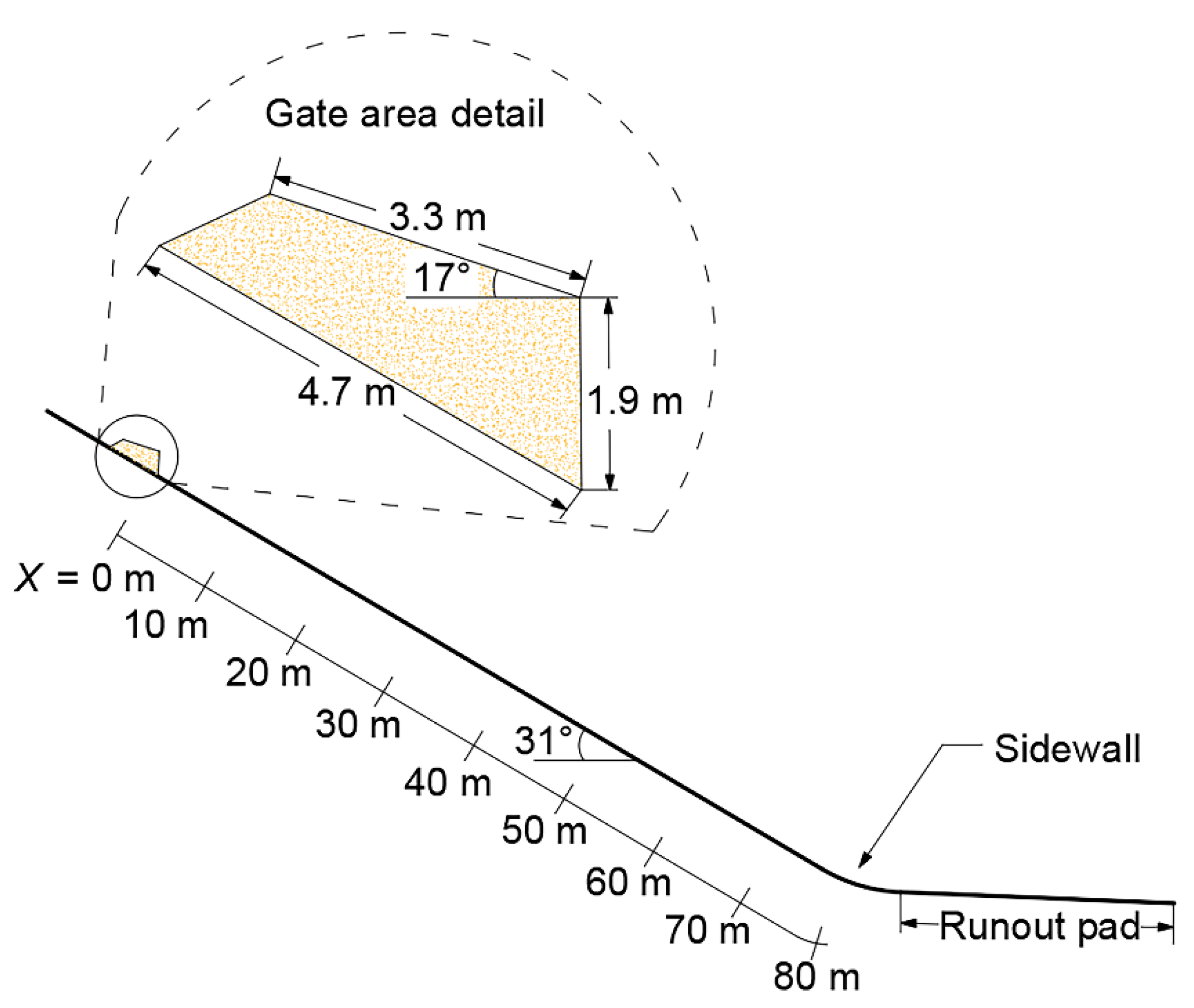
3.1. Case Description
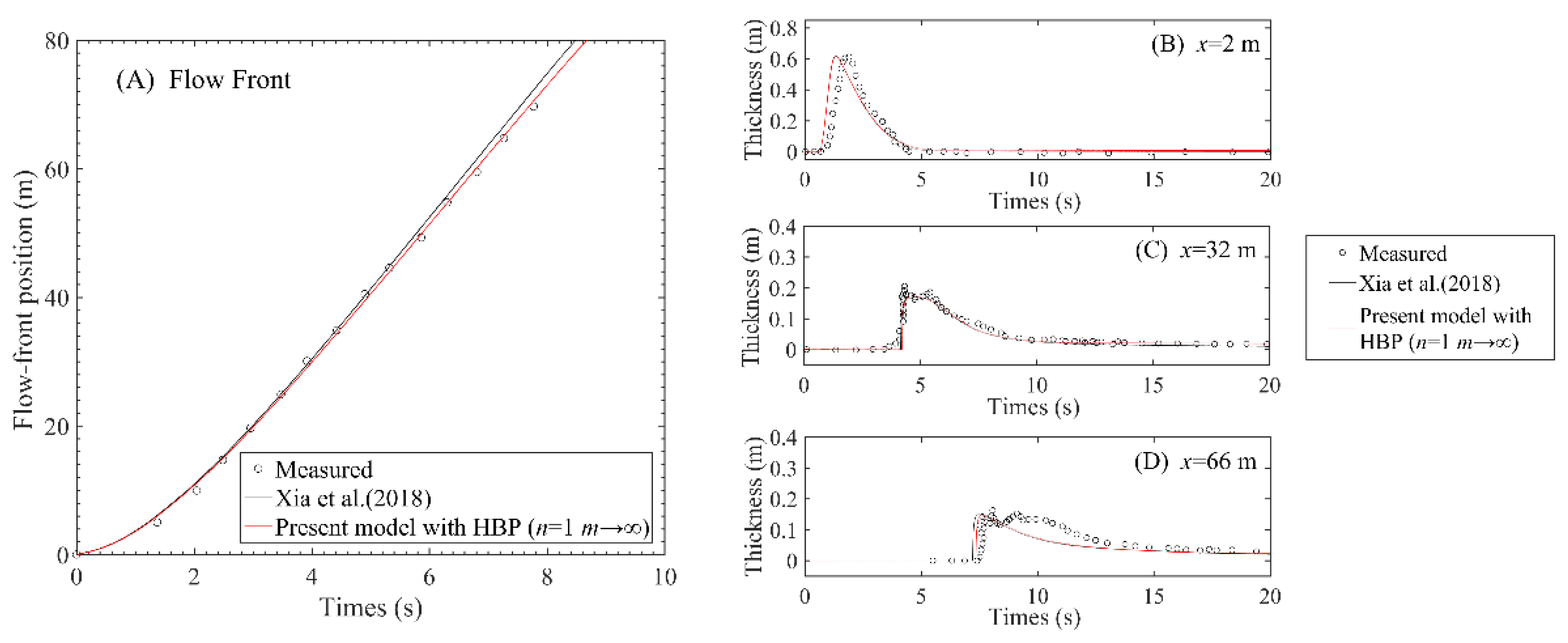
The 95 m long, 2 m wide, and 1.2 m deep flume with a uniform bed slope of 31 degrees throughout most of its length was applied, the schematic flume geometry is shown in Figure 1. A 2 m high vertical headgate used to retain static debris prior to its release was set to be the reference of longitudinal distances, i.e., x = 0 m. At x = 74 m, the flume bed begins to flatten [46]. The flow-front positions were tracked, and the flow thickness at three cross-sections of the uniformly sloping flume located at x = 2 m, 32 m, and 66 m were also measured. Initially, approximately 10 m3 of sand-gravel-mud mixture debris were released by the sudden opening of the two-piece steel headgate. They moved across the smooth bed from x = 0 to 6 m with the basal friction angle of 28° and then the rough bed after x = 6 m with the basal friction angle of 40°.
The present study mainly uses a one-dimensional model to simulate the debris-flow evolution; therefore, the computational domain consists of the uniformly sloping flume and the adjacent runout pad that is considered to have the same width as the flume. The numerical simulations are performed within the time period before the forward and backward waves reach the downstream and upstream boundaries, respectively; thus, the boundary conditions can be simply set according to the initial status.
The detailed grain-size distribution of the debris can be obtained according to Iverson et al. (2010) [46]. The coefficients in closure models of bed shear stresses, sediment entrainment and deposition, and stresses due to fluctuations are all the same as Xia et al. (2018) [7]. For effective viscosity, the dynamic viscosity for Newtonian fluid is set to be μ N = 0.001   P a s . First, we used the simplified HBP model with n = 1, m (i.e., Bingham model) to evaluate the effect of rheological relation.

3.2. Results

Figure 2A shows the computed flow front position of debris flows by the present model with HBP rheological relation and its comparison with simulations by Xia et al. (2018) [7] along with the measured data. It is noted that with the coefficients n = 1, m , the HBP model can be simplified to Bingham fluid. Even so, the improved performance on front tracking is obvious, especially after about t = 4.5 s. This reveals that the effect of rheological features of the debris delays the arrival of the flow front as the debris flow propagates. Figure 2B–D illustrate the predicted flow thicknesses of the present model closed by HBP model compared with the observed data and the available computed results by Xia et al. (2018) [7]. Just downslope from the flume headgate at x = 2 m, the computed flow depths are almost the same (Figure 2B), so the rheological feature may not show its impact at this time. As the propagation of the debris flow, the stress–strain relationship due to the interaction forces of internal debris flow, described by the HBP model, contributes to a better agreement with the measured flow thickness as compared to Xia et al. (2018) [7] at cross-sections x = 32 and 66 m. It is noted that thickest flow depth lasts about 2.5 s for measurement while only 0.5 s for computation results at x = 66 m. This may be due to the effect of interphase (water-to-sediment) and particle–particle interactions of debris flow cannot be fully expressed by the mixture model. The flow front arrival points and the steady state after about t = 10 s are closer to the measured data.

4. Discussion

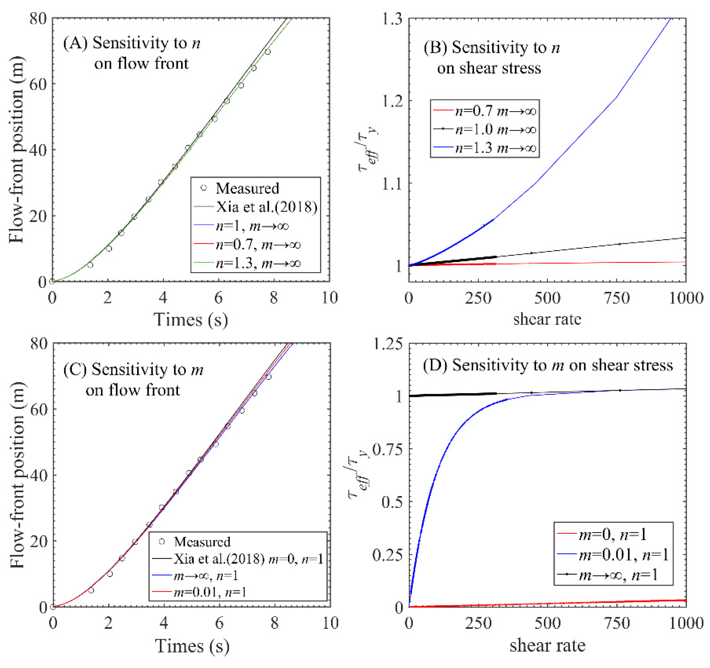
4.1. Sensitivity Analysis

Flow front and shear stress are two important factors to judge whether a numerical model can successfully simulate the main characteristics of debris flow or not. Hence, it is interesting to investigate the sensitivity of the simulation results by the present model to coefficients n and m. First, m is set to be infinity, and n is tuned by 30% to check its effect on the results. Then, n is set to be 1, and the results of the track of flow front are computed by m = 0, 0.01 and infinity, respectively.
Figure 3A compares the computed flow front positions with the measured data. It seems that the results by the model with different n are almost overlapped despite the improvement compared to Xia et al. (2018) [7]. According to Equation (6), the ratio of shear stress τ e f f to yield stress τ y can be written as:
τ e f f τ y = μ τ y γ ˙ n + 1 e m γ ˙
n reflects the shear-thinning (n < 1) and shear-thickening (n > 1) behavior of a non-Newtonian fluid, as shown in Figure 3B. With the variation of shear rate γ ˙ , the ratio of shear stress τ e f f to yield stress τ y shows a linear relationship when n = 1, while the ratio increases if n > 1 and decreases if n < 1 when shear rate γ ˙ is over 1. Furthermore, from Figure 3B, the coefficient n mainly controls the linear or nonlinear behavior in the high shearing rate range, while the most values of shear rate in this study case are below 300 with limit differences among shear stress S τ e f f , which indicates the little effects on the flow front tracking (Figure 3A) due to tuned n. When n = 1, m = 0 and infinity form the result interval of flow front position, and m = 0.01 is in between, shown in Figure 3C. As the m gets smaller, the computed results are closer to that of Newtonian model. Notably, when n = 1 and m = 0, stress–strain relationship is reduced to Newtonian model (red line in Figure 3D), and when n = 1 and m , stress–strain relationship is reduced to Bingham model τ e f f τ y = μ τ y γ ˙ + 1 (black line in Figure 3D), and the coefficient m mainly controls the initial rapid growth of shearing stress.
The L 1 norm of flow front location is deployed to quantify the impacts of m and n on debris-flow modeling, as shown in Table 1. The L 1 norm is defined as L 1 = | x f x f * | / x f * × 100 % , where x f = computed flow front location; x f * = measured flow front location. The L 1 norms of tuned n are almost the same, which is consistent with the results shown in Figure 3A. The L 1 value of flow front simulation with Newtonian model (n = 1, m = 0) is 2.56. It is bigger than the results using the non-Newtonian model, which are 2.03 and 1.702 for m = 0.01 and m , respectively.
Generally, the coefficient n has limited influence on flow front simulation, maybe due to the scale of the experiment and the composition of the sediment. However, considering the non-Newtonian model can improve the accuracy of the model in tracking the flow front.

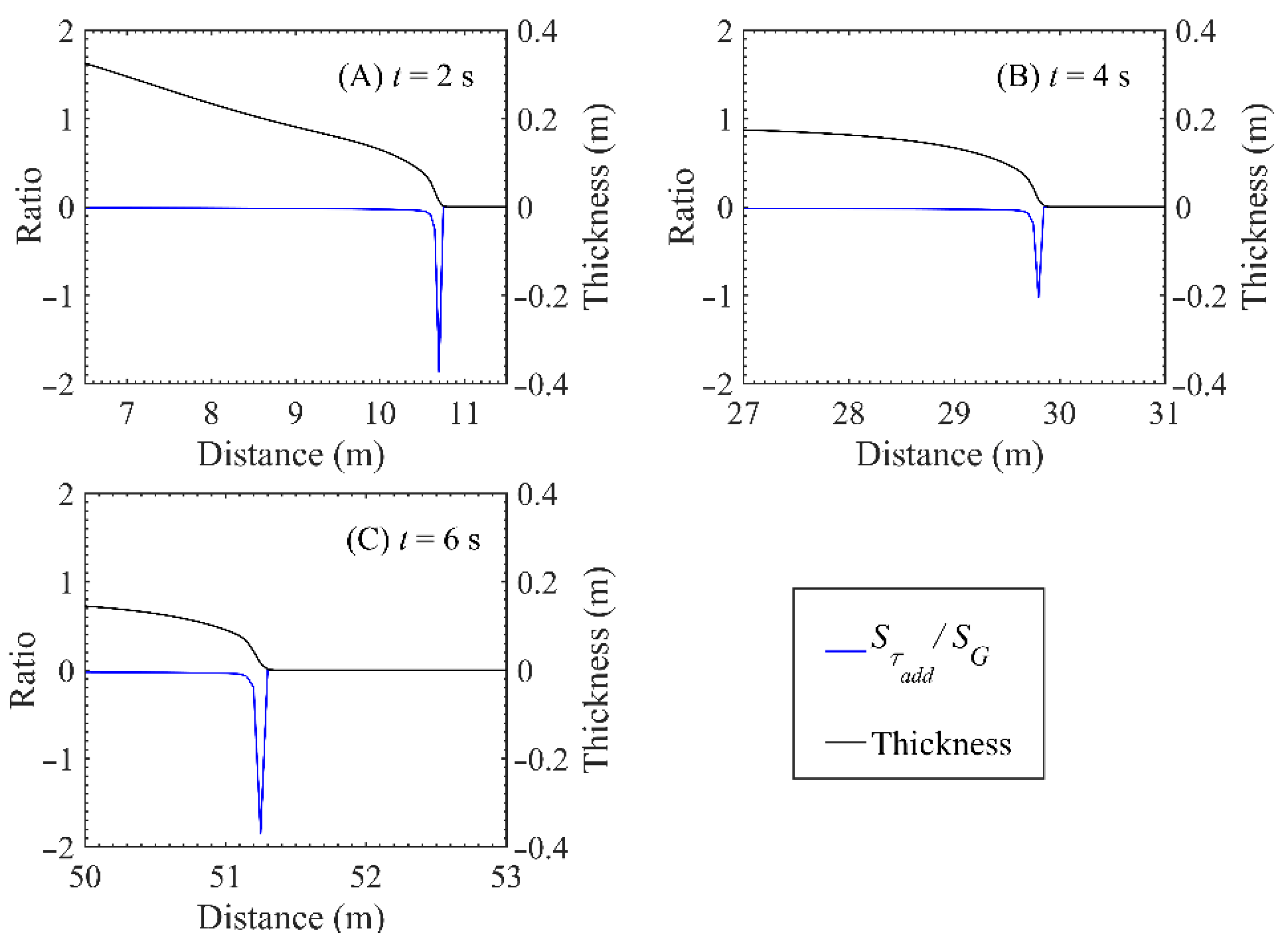
4.2. Effects of Additional Shear Stress Due to Non-Newtonian Fluid

Compared to the model of Xia et al. (2018) [7], based on Newtonian fluid assumption, the present model includes the additional shear stress τ a d d to describe the rheological features of debris flows, which actually is the difference between viscosity of non-Newtonian fluid (i.e., μ e f f ) and Newtonian fluid (i.e., μ N ). To provide insight into the contributions of the rheological features of the non-Newtonian fluid to debris-flow modeling shown by the additional shear stress, the spatial distribution ratios of S τ e f f / S G ( S τ e f f = τ a d d ; S G = ρ m g z h ) at specific instants along with the flow thicknesses are present, as shown in Figure 4. It illustrates that the ratio is negative around the flow front. Although the value is little from the trough to the peak of the debris flow, it is considerable around the debris-flow front, and the additional shear stress S τ e f f is by no means negligible compared with the gravitational term S G . This effect is similar to that of stress terms due to fluctuations in Xia et al. (2018) [7], and their effects are almost at the same level as the ratios and have the same order of magnitude (Figure 9 in Xia et al. (2018) [7] compared to Figure 4 in present paper).

5. Conclusions

Under the framework of shallow water hydro-sediment-morphodynamics, a complete numerical model for debris flow is proposed. Unlike some previous simplified models, the present model not only incorporates the effect of rheological features of the non-Newtonian fluid but also explicitly accommodates the interactions between flow, non-uniform sediment transport, and bed evolution. This promotes the accuracy of debris-flow modeling from a theoretical perspective. A fully conservative numerical algorithm is used to solve the governing equations. The hyperbolic system that can be readily solved by many existing schemes is disrupted due to the fluctuation stress. The explicit finite volume discretization combined with the implicit discretization method is applied to solve this mathematical problem by efficient in-house program code. It lays the foundation for application to both laboratory and field-scale debris-flow modeling.
One set of large-scaled U.S. Geological Survey debris-flow experiments was applied to investigate the non-Newtonian fluid on debris-flow modeling. Hersch–Bulkley–Papanastasiou model is used to estimate the rheological feature of debris flow because it is more generalized and considered suitable for describing the nonlinear features of debris flow. It is found that the present model closed by HBP model performs better than the existing quasi-single-phase mixture model. The coefficients n and m in the HBP model are discussed. The results illustrate that the coefficient n plays a role in the high shearing rate range, while the coefficient m has effects on the initial growth of shearing stress. Besides, the additional shear stress due to non-Newtonian fluid is also investigated, and it cannot be negligible as compared with the gravitational term.
Further studies are needed to be carried out because the rheological features may be varied due to the composition of sediments, soil moisture, and even the scale of debris flows. More suitable stress–strain relationships are desiderated to be found. Besides, 2-dimensional model can be extended in the near future.

Author Contributions

Conceptualization, C.X.; methodology, C.X.; validation, H.T.; writing—original draft preparation, C.X. and H.T.; writing—review and editing, C.X. and H.T. All authors have read and agreed to the published version of the manuscript.

Funding

This research was funded by the National Natural Science Foundation of China, grant number 12002310.

Institutional Review Board Statement

Not applicable.

Informed Consent Statement

Not applicable.

Data Availability Statement

Not applicable.

Conflicts of Interest

The authors declare no conflict of interest.

References

  1. Takahashi, T. Debris Flow Mechanics, Prediction and Countermeasures; Taylor & Francis: London, UK, 2007. [Google Scholar]
  2. Le, M. Dynamic Mechanism of Gully-Type Debris Flow and Its Numerical Simulation; China Institute of Water Resources and Hydropower Research: Beijing, China, 2019. [Google Scholar]
  3. Hu, K.; Cui, P.; Li, P. Debris flow dynamic models and numerical computation. Chin. J. Nat. 2014, 36, 313–318. (In Chinese) [Google Scholar]
  4. Hu, K.; Cui, P.; Tian, M.; Yang, H. A review of the debris flow dynamic models and numerical simulation. J. Hydraul. Eng. 2012, 43, 79–84. (In Chinese) [Google Scholar] [CrossRef]
  5. Brufau, P.; Garcia-Navarro, P.; Ghilardi, P.; Natale, L.; Savi, F. 1D mathematical modelling of debris flow. J. Hydraul. Res. 2000, 38, 435–446. [Google Scholar] [CrossRef]
  6. Pudasaini, S.; Wang, Y.; Hutter, K. Modelling debris flows down general channels. Nat. Hazards Earth Syst. Sci. 2005, 5, 799–819. [Google Scholar] [CrossRef]
  7. Xia, C.; Li, J.; Cao, Z.; Liu, Q.; Hu, K. A quasi single-phase model for debris flows and its comparison with a two-phase model. J. Mt. Sci. 2018, 15, 1071–1089. [Google Scholar] [CrossRef]
  8. Pelanti, M.; Bouchut, F.; Mangeney, A. A Roe-Type scheme for two-phase shallow granular flows over variable topography. ESAIM-Math. Model. Num. 2008, 42, 851–885. [Google Scholar] [CrossRef] [Green Version]
  9. Pitman, E.; Le, L. A two-fluid model for avalanche and debris flows. Philos. Trans. R. Soc. A 2005, 363, 1573–1601. [Google Scholar] [CrossRef]
  10. Di Cristo, C.; Greco, M.; Iervolino, M.; Leopardi, A.; Vacca, A. Two-dimensional two-phase depth-integrated model for transients over mobile bed. J. Hydraul. Eng. 2016, 142, 04015043. [Google Scholar] [CrossRef] [Green Version]
  11. Li, J.; Cao, Z.; Hu, K.; Pender, G.; Liu, Q. A depth-averaged two-phase model for debris flows over fixed beds. Int. J. Sediment Res. 2018, 33, 362–477. [Google Scholar] [CrossRef]
  12. Li, J.; Cao, Z.; Hu, K.; Pender, G.; Liu, Q. A depth-averaged two-phase model for debris flows over erodible beds. Earth Surf. Process. Landf. 2018, 43, 817–839. [Google Scholar] [CrossRef]
  13. Denlinger, R.; Iverson, R. Flow of variably fluidized granular masses across three-dimensional terrain: 2. Numerical predictions and experimental tests. J. Geophys. Res. Solid Earth 2001, 106, 553–566. [Google Scholar] [CrossRef]
  14. Liu, K.; Huang, M. Numerical simulation of debris flow with application on hazard area mapping. Comput. Geosci. 2006, 10, 221–240. [Google Scholar] [CrossRef]
  15. Armanini, A.; Fraccarollo, L.; Rosatti, G. Two-dimensional simulation of debris flows in erodible channels. Comput. Geosci. 2009, 35, 993–1006. [Google Scholar] [CrossRef]
  16. Rosatti, G.; Begnudelli, L. Two-dimensional simulation of debris flows over mobile bed: Enhancing the TRENT2D model by using a well-balanced Generalized Roe-type solver. Comput. Fluids. 2013, 71, 179–195. [Google Scholar] [CrossRef]
  17. Shieh, C.; Jan, C.; Tsai, Y. A numerical simulation of debris flow and its application. Nat. Hazards 1996, 13, 39–54. [Google Scholar] [CrossRef]
  18. Armanini, A.; Capart, H.; Fraccarollo, L.; Larcher, M. Rheological stratification in experimental free-surface flows of granular-liquid mixtures. J. Fluid Mech. 2005, 532, 269–319. [Google Scholar] [CrossRef] [Green Version]
  19. Pastor, M.; Blanc, T.; Haddad, B.; Petrone, S.; Sanchez, M.; Drempetic, V.; Nissler, D.; Crosta, G.; Cascini, L.; Sorbino, G.; et al. Application of a SPH depth-integrated model to landslide run-out analysis. Landslides 2014, 11, 793–812. [Google Scholar] [CrossRef] [Green Version]
  20. Huang, Y.; Zhang, W.; Xu, Q.; Xie, P.; Liang, H. Run-out analysis of flow-like landslides triggered by the Ms 8.0 2008 Wenchuan earthquake using smoothed particle hydrodynamics. Landslides 2012, 9, 275–283. [Google Scholar] [CrossRef]
  21. Barnes, H.; Hutton, J.; Walters, K. An Introduction to Rheology; Rheology Series 3; Elsevier: Amsterdam, The Netherlands, 1989. [Google Scholar]
  22. Wang, W.; Chen, G.; Han, Z.; Zhou, S.; Zhang, H.; Jing, P. 3D numerical simulation of debris-flow motion using SPH method incorporating non-Newtonian fluid behavior. Nat. Hazards 2016, 81, 1981–1998. [Google Scholar] [CrossRef]
  23. Jeon, C.; Hodges, B. Comparing thixotropic and Herschel-Bulkley parameterizations for continuum models of avalanches and subaqueous debris flows. Nat. Hazards Earth Syst. Sci. 2018, 18, 303–319. [Google Scholar] [CrossRef] [Green Version]
  24. Papanastasiou, T. Flows of materials with yield. J. Rheol. 1987, 31, 385–404. [Google Scholar] [CrossRef]
  25. Han, Z.; Su, B.; Li, Y.; Wang, W.; Wang., W.; Huang, J.; Chen, G. Numerical simulation of debris-flow behavior based on the SPH method incorporating the Herschel-Bulkley-Papanastasiou rheology model. Eng. Geol. 2019, 255, 26–36. [Google Scholar] [CrossRef]
  26. Major, J.J.; Pierson, T.C. Debris flow rheology: Experimental analysis of finegrained slurries. Water Resour. Res. 1992, 28, 841–857. [Google Scholar] [CrossRef]
  27. Jeffrey, D.P.; Kelin, X.W.; Alessandro, S. Experimental study of the grain-flow, fluid-mud transition in debris flows. J. Geol. 2001, 109, 427–447. [Google Scholar] [CrossRef] [Green Version]
  28. Pudasaini, S.P. Some exact solutions for debris and avalanche flows. Phys. Fluids 2011, 23, 043301. [Google Scholar] [CrossRef]
  29. Pasculli, A.; Minatti, L.; Sciarra, N.; Paris, E. SPH modeling of fast muddy debris flow: Numerical and experimental comparison of certain commonly utilized approaches. Ital. J. Geosci. 2013, 132, 350–365. [Google Scholar] [CrossRef] [Green Version]
  30. Hirano, M. River bed degradation with armouring. Proc. Jpn. Soc. Civ. Eng. 1971, 1971, 55–65. [Google Scholar] [CrossRef] [Green Version]
  31. Cao, Z.; Xia, C.; Pender, G.; Liu, Q. Shallow water hydro-sediment-morphodynamic equations for fluvial processes. J. Hydraul. Eng. 2017, 143, 02517001. [Google Scholar] [CrossRef]
  32. Lucas, A.; Mangeney, A.; Ampuero, J. Frictional velocity-weakening in landslides on Earth and on other planetary bodies. Nat. Commum. 2014, 5, 417. [Google Scholar] [CrossRef] [Green Version]
  33. Pirulli, M.; Pastor, M. Numerical study on the entrainment of bed material into rapid landslides. Geotechnique 2012, 62, 959–972. [Google Scholar] [CrossRef]
  34. Richardson, J.; Zaki, W. Sedimentation and fluidisation: Part 1. Chem. Eng. Res. Des. 1954, 75, s82–s99. [Google Scholar] [CrossRef]
  35. Wu, W.; Wang, S.; Jia, Y. Nonuniform sediment transport in alluvial rivers. J. Hydraul. Res. 2000, 38, 427–434. [Google Scholar] [CrossRef]
  36. Zhang, R.; Xie, J. Sedimentation Research in China-Systematic Selections; Water and Power Press: Beijing, China, 1993. (In Chinese) [Google Scholar]
  37. Cao, Z.; Hu, P.; Hu, K.; Pender, G.; Liu, Q. Modelling roll waves with shallow water equations and turbulent closure. J. Hydraul. Res. 2015, 53, 161–177. [Google Scholar] [CrossRef] [Green Version]
  38. Rastogi, A.; Rodi, W. Predictions of heat and mass transfer in open channels. J. Hydraul. Div. 1978, 104, 397–420. [Google Scholar] [CrossRef]
  39. Ni, H. Turbulence Simulation and Application in Modern Hydraulics Engineering; China Water Power Press: Beijing, China, 2010. [Google Scholar]
  40. Iverson, R. Landslide triggering by rain infiltration. Water Resour. Res. 2000, 36, 1897–1910. [Google Scholar] [CrossRef] [Green Version]
  41. Wang, J. Effects of constitutive relations on turbidity current evolutions. In Proceedings of the 37th IAHR World Congress, Kuala Lumpur, Malaysia, 13–18 August 2017; pp. 1047–1057. [Google Scholar]
  42. Fei, X. A Model for Calculating Viscosity of Sediment Carrying Flow in the Middle and Lower Yellow River. J. Sediment Res. 1991, 2, 1–13. [Google Scholar] [CrossRef]
  43. Aureli, F.; Maranzoni, A.; Mignosa, P.; Ziveri, C. A weighted surface-depth gradient method for the numerical integration of the 2D shallow water equations with topography. Adv. Water Resour. 2008, 31, 962–974. [Google Scholar] [CrossRef]
  44. Xia, C.; Cao, Z.; Pender, G.; Borthwick, A. Numerical Algorithms for Solving Shallow Water Hydro-Sediment-Morphodynamic Equations. Eng. Comput. 2017, 34, 2836–2861. [Google Scholar] [CrossRef] [Green Version]
  45. Iverson, R. The physics of debris flows. Rev. Geophys. 1997, 35, 245–296. [Google Scholar] [CrossRef] [Green Version]
  46. Iverson, R.; Logan, M.; LaHusen, R.; Berti, M. The perfect debris flow? Aggregated results from 28 large-scale experiments. J. Geophys. Res. Earth Surf. 2010, 115, F03005. [Google Scholar] [CrossRef]
  47. Iverson, R.; Reid, M.; Logan, M.; LaHusen, R.; Godt, J.; Griswold, J. Positive feedback and momentum growth during debris-flowentrainment of wet bed sediment. Nat. Hazards 2011, 4, 116–121. [Google Scholar] [CrossRef]
Figure 1. Schematic flume geometry of the debris-flow experiment.
Water 14 01369 g001
Figure 2. Computed results by Xia et al. (2018) [7] and present model with HBP model. (A) Flow front tracking; (B) flow thickness at x = 2 m; (C) flow thickness at x = 32 m; (D) flow thickness at x = 66 m.
Water 14 01369 g002
Figure 3. Sensitivity to coefficients n and m. (A) Flow front sensitivity to n; (B) shear stress sensitivity to n; (C) flow front sensitivity to m; (D) shear stress sensitivity to m.
Water 14 01369 g003
Figure 4. The ratios of the additional shear stress to the gravitational term along with the flow thicknesses at several instants. (A) t = 2 s; (B) t = 4 s; (C) t = 6 s.
Water 14 01369 g004
Table 1. L1 norm of the HBP model with tuned n and m.
Coefficient Value n   ( m ) m (n = 1)
0.71.01.300.01
L 1 (%)1.7021.7021.7032.562.0301.702
Publisher’s Note: MDPI stays neutral with regard to jurisdictional claims in published maps and institutional affiliations.

