
A Review on Interpretable and Explainable Artificial Intelligence in Hydroclimatic Applications


 ,
, 
Abstract
:1. Introduction
- Which predictors and predictands are used in the IAI-based analysis? What is the size, type (e.g., static or time-variant), and sampling interval of multidimensional input data? Are the chosen predictors representative of the underlying physics of the problem tackled? Is the use of surrogate variables in IAI-based analyses acceptable for the regions with scarce data?
- Are the explanatory methods properly and effectively coupled with the AI models (leading to XAI models) to assess the importance of the predictors in predictions, explain the interdependencies and interrelations between the predictors in estimating the predictands, justify the IAI-based decisions, and explore new knowledge?
- Are class imbalances properly addressed in categorical IAI and XAI modeling applications?
- Under what conditions could in-depth domain knowledge become critical? Would domain knowledge allow flexibility for the choice of predictive variables in IAI/XAI-based analyses?
- Should multiple IAI/XAI models be used independently or should the results from multiple IAI/XAI models be a weighted-average? Can IAI/XAI and non-IAI models be used in a hybrid form to enhance prediction accuracy? How do prediction performances of IAI/XAI and non-IAI models compare in different domains with different data types and sizes?
- Are there any attempts toward interventional XAI modeling in hydroclimatic applications to relax the nonstationary assumption in AI-based analyses?
- How do IAI/XAI models perform against physics-based models? Are there applications, in which IAI/XAI models fail to provide reliable results?
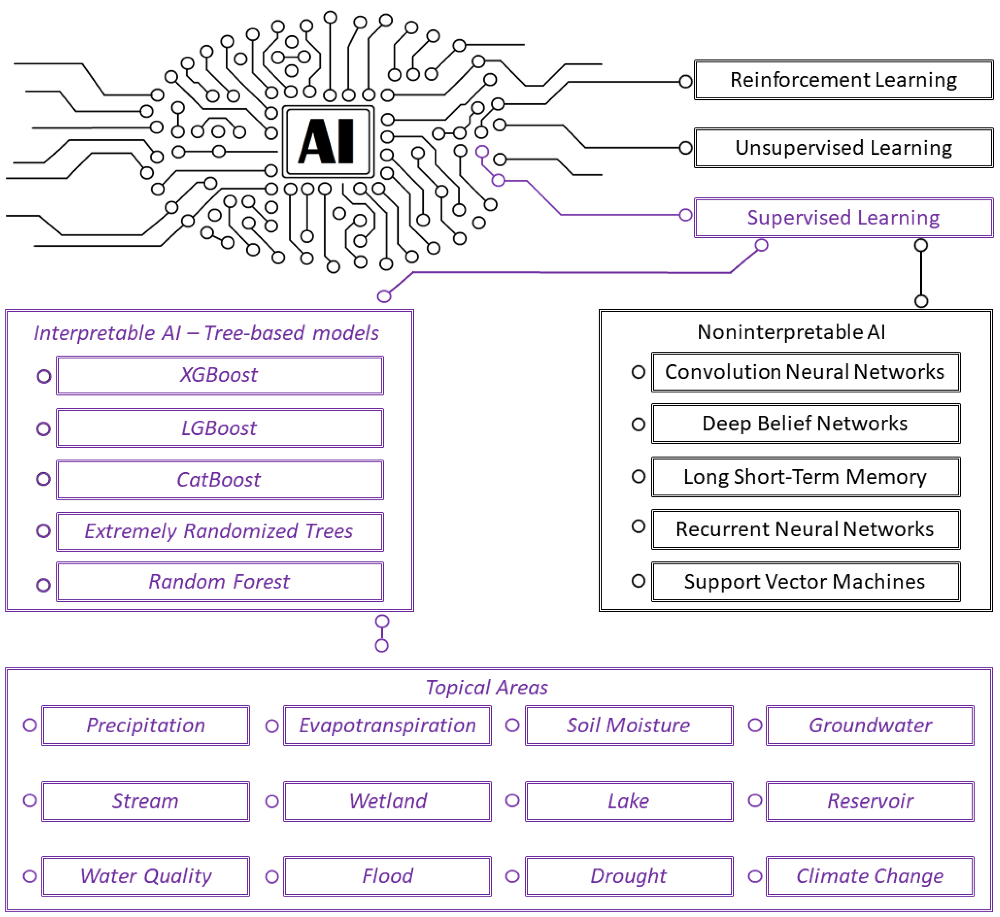
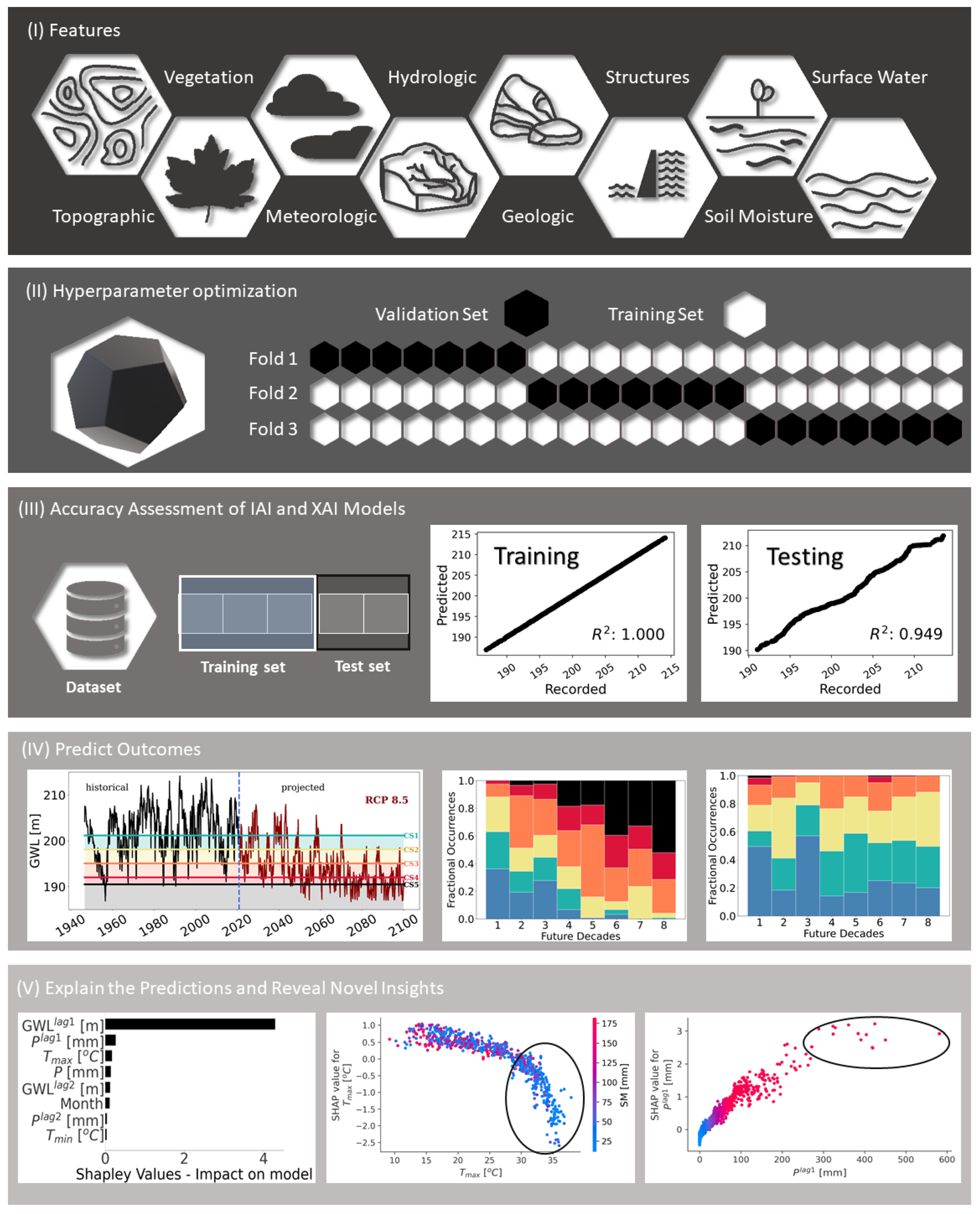
2. IAI and XAI Models
3. Tree-Based Ensemble IAI Models Considered in This Review
4. IAI and XAI Applications in Hydroclimatic Domains
4.1. Data Imputations Using IAI Models
4.2. Hydroclimatic Predictions Using IAI and XAI Models
4.2.1. Evapotranspiration Predictions
4.2.2. Precipitation Predictions
4.2.3. Soil Moisture Predictions
4.2.4. Groundwater Potential Predictions
4.2.5. Groundwater Level Predictions
4.2.6. Streamflow Predictions
4.2.7. Water Level Predictions in Reservoirs, Lakes, and Delineation of Wetlands
4.2.8. Water Quality Predictions
4.2.9. Flood Hazard Risks Prediction
4.2.10. Drought Predictions
4.2.11. Climate Change Impacts Modeling
5. Discussion and Conclusions
Author Contributions
Funding
Institutional Review Board Statement
Informed Consent Statement
Data Availability Statement
Acknowledgments
Conflicts of Interest
Abbreviations
| Artificial Intelligence Models: | |
| AdaBoost | Adaptive Boosting |
| ANN | Artificial Neural Networks |
| CNN | Convolutional Neural Network |
| DL | Deep Learning |
| DT | Decision Trees |
| GBoost | Gradient Boosting |
| IAI | Interpretable Artificial Intelligence |
| LIME | Local Interpretable Model-agnostic Explanations |
| LSTM | Long Short Term Memory |
| LR | Linear Regression |
| AI | Artificial Intelligence |
| MLP | Multi-layer Perceptron |
| XGBoost | Natural Gradient Boosting |
| RF | Random forest |
| SHAP | SHaply Additive Explanation |
| SVM | Support Vector Machine |
| SVR | Support Vector Regression |
| XGBoost | Extreme Gradient Boosting |
| XAI | Explainable Artificial Intelligence |
| Key Variables: | |
| Evapotranspiration | |
| Actual evapotranspiration | |
| Reference crop evapotranspiration | |
| Groundwater level | |
| Groundwater potential | |
| P | Precipitation |
| Atmospheric pressure | |
| Streamflow | |
| Shortwave solar radiation | |
| Soil moisture | |
| Air temperature | |
| Water surface temperature | |
| Wind speed | |
| Water level |
References
- Ochoa-Tocachi, B.F.; Buytaert, W.; Antiporta, J.; Acosta, L.; Bardales, J.D.; Célleri, R.; Crespo, P.; Fuentes, P.; Gil-Ríos, J.; Guallpa, M.; et al. High-resolution hydrometeorological data from a network of headwater catchments in the tropical Andes. Sci. Data 2018, 5, 180080. [Google Scholar] [CrossRef] [PubMed]
- Singh, V.P. Hydrologic modeling: Progress and future directions. Geosci. Lett. 2018, 5, 15. [Google Scholar] [CrossRef]
- Adamala, S. An Overview of Big Data Applications in Water Resources Engineering. Mach. Learn. Res. 2017, 2, 10–18. [Google Scholar] [CrossRef]
- Obermeyer, Z.; Emanuel, E.J. Predicting the Future—Big Data, Machine Learning, and Clinical Medicine. N. Engl. J. Med. 2016, 375, 1216–1219. [Google Scholar] [CrossRef] [Green Version]
- Biran, O.; Cotton, C.V. Explanation and Justification in Machine Learning: A Survey. IJCAI 2017 Workshop on Explainable Artificial Intelligence. 2017. Available online: http://www.cs.columbia.edu/~orb/papers/xai_survey_paper_2017.pdf (accessed on 19 February 2022).
- Miller, T. Explanation in artificial intelligence: Insights from the social sciences. Artif. Intell. 2019, 267, 1–38. [Google Scholar] [CrossRef]
- Roscher, R.; Bohn, B.; Duarte, M.F.; Garcke, J. Explainable Machine Learning for Scientific Insights and Discoveries. IEEE Access 2020, 8, 42200–42216. [Google Scholar] [CrossRef]
- Adadi, A.; Berrada, M. Peeking Inside the Black-Box: A Survey on Explainable Artificial Intelligence (XAI). IEEE Access 2018, 6, 52138–52160. [Google Scholar] [CrossRef]
- Zounemat-Kermani, M.; Batelaan, O.; Fadaee, M.; Hinkelmann, R. Ensemble machine learning paradigms in hydrology: A review. J. Hydrol. 2021, 598, 126266. [Google Scholar] [CrossRef]
- Guidotti, R.; Monreale, A.; Ruggieri, S.; Turini, F.; Pedreschi, D.; Giannotti, F. A Survey of Methods for Explaining Black Box Models. ACM Comput. Surv. 2018, 51, 93. [Google Scholar] [CrossRef] [Green Version]
- Shapley, L. A value for n-person games. Contrib. Theory Games 1953, 307–317. [Google Scholar]
- Lundberg, S.M.; Erion, G.; Chen, H.; DeGrave, A.; Prutkin, J.M.; Nair, B.; Katz, R.; Himmelfarb, J.; Bansal, N.; Lee, S.I. From local explanations to global understanding with explainable AI for trees. Nat. Mach. Intell. 2020, 2, 2522–5839. [Google Scholar] [CrossRef] [PubMed]
- Ribeiro, M.T.; Singh, S.; Guestrin, C. “Why should I trust you?” Explaining the predictions of any classifier. In Proceedings of the 22nd ACM SIGKDD International Conference on Knowledge Discovery and Data Mining, San Francisco, CA, USA, 13–17 August 2016; pp. 1135–1144. [Google Scholar]
- Xie, Y.R.; Castro, D.C.; Bell, S.E.; Rubakhin, S.S.; Sweedler, J.V. Single-Cell Classification Using Mass Spectrometry through Interpretable Machine Learning. Anal. Chem. 2020, 92, 9338–9347. [Google Scholar] [CrossRef] [PubMed]
- Rodríguez-Pérez, R.; Bajorath, J. Interpretation of machine learning models using shapley values: Application to compound potency and multi-target activity predictions. J. Comput. Aided Mol. Des. 2020, 34, 1013–1026. [Google Scholar] [CrossRef] [PubMed]
- Mangalathu, S.; Hwang, S.H.; Jeon, J.S. Failure mode and effects analysis of RC members based on machine-learning-based SHapley Additive exPlanations (SHAP) approach. Eng. Struct. 2020, 219, 110927. [Google Scholar] [CrossRef]
- Başağaoğlu, H.; Chakraborty, D.; Winterle, J. Reliable Evapotranspiration Predictions with a Probabilistic Machine Learning Framework. Water 2021, 13, 557. [Google Scholar] [CrossRef]
- Chakraborty, D.; Başağaoğlu, H.; Winterle, J. Interpretable vs. noninterpretable machine learning models for data-driven hydro-climatological process modeling. Expert Syst. Appl. 2021, 170, 114498. [Google Scholar] [CrossRef]
- Chakraborty, D.; Ivan, C.; Amero, P.; Khan, M.; Rodriguez-Aguayo, C.; Başağaoğlu, H.; Lopez-Berestein, G. Explainable Artificial Intelligence Reveals Novel Insight into Tumor Microenvironment Conditions Linked with Better Prognosis in Patients with Breast Cancer. Cancers 2021, 13, 3450. [Google Scholar] [CrossRef]
- Chakraborty, D.; Başağaoğlu, H.; Gutierrez, L.; Mirchi, A. Explainable AI reveals new hydroclimatic insights for ecosystem-centric groundwater management. Environ. Res. Lett. 2021, 16, 114024. [Google Scholar] [CrossRef]
- Chakraborty, D.; Alam, A.; Chaudhuri, S.; Başağaoğlu, H.; Sulbaran, T.; Langar, S. Scenario-based prediction of climate change impacts on building cooling energy consumption with explainable artificial intelligence. Appl. Energy 2021, 291, 116807. [Google Scholar] [CrossRef]
- Li, L.; Qiao, J.; Yu, G.; Wang, L.; Li, H.Y.; Liao, C.; Zhu, Z. Interpretable tree-based ensemble model for predicting beach water quality. Water Res. 2022, 211, 118078. [Google Scholar] [CrossRef]
- Wang, D.; Thunéll, S.; Lindberg, U.; Jiang, L.; Trygg, J.; Tysklind, M. Towards better process management in wastewater treatment plants: Process analytics based on SHAP values for tree-based machine learning methods. J. Environ. Manag. 2022, 301, 113941. [Google Scholar] [CrossRef] [PubMed]
- Linardatos, P.; Papastefanopoulos, V.; Kotsiantis, S. Explainable AI: A Review of Machine Learning Interpretability Methods. Entropy 2021, 23, 18. [Google Scholar] [CrossRef] [PubMed]
- Lipton, Z.C. The Mythos of Model Interpretability: In Machine Learning, the Concept of Interpretability is Both Important and Slippery. Queue 2018, 16, 31–57. [Google Scholar] [CrossRef]
- Rudin, C. Stop explaining black box machine learning models for high stakes decisions and use interpretable models instead. Nat. Mach. Intell. 2019, 1, 206–215. [Google Scholar] [CrossRef] [Green Version]
- Eschenbach, W.J. Transparency and the Black Box Problem: Why We Do Not Trust AI. Philos. Technol. 2021, 34, 1607–1622. [Google Scholar] [CrossRef]
- D’Isanto, A.; Cavuoti, S.; Gieseke, F.; Polsterer, K.L. Return of the features—Efficient feature selection and interpretation for photometric redshifts. Astron. Astrophys. 2018, 616, A97. [Google Scholar] [CrossRef] [Green Version]
- Makridakis, S.; Spiliotis, E.; Assimakopoulos, V. Statistical and Machine Learning forecasting methods: Concerns and ways forward. PLoS ONE 2018, 13, e0194889. [Google Scholar] [CrossRef] [Green Version]
- Shin, D. The effects of explainability and causability on perception, trust, and acceptance: Implications for explainable AI. Int. J. Hum.-Comput. Stud. 2021, 146, 102551. [Google Scholar] [CrossRef]
- Amann, J.; Blasimme, A.; Vayena, E.; Frey, D.; Madai, V.I. Explainability for artificial intelligence in healthcare: A multidisciplinary perspective. BMC Med. Inform. Decis. Mak. 2020, 20, 310. [Google Scholar] [CrossRef]
- London, A.J. Artificial Intelligence and Black-Box Medical Decisions: Accuracy versus Explainability. Hastings Cent. Rep. 2019, 49, 15–21. [Google Scholar] [CrossRef]
- Bedi, S.; Samal, A.; Ray, C.; Snow, D. Comparative evaluation of machine learning models for groundwater quality assessment. Environ. Monit. Assess. 2020, 192, 776. [Google Scholar] [CrossRef] [PubMed]
- Ravindran, S.; Bhaskaran, S.; Ambat, S. A Deep Neural Network Architecture to Model Reference Evapotranspiration Using a Single Input Meteorological Parameter. Environ. Process 2021, 103, 1567–1599. [Google Scholar] [CrossRef]
- Wen, Y.; Zhao, J.; Zhu, G.; Xu, R.; Yang, J. Evaluation of the RF-Based Downscaled SMAP and SMOS Products Using Multi-Source Data over an Alpine Mountains Basin, Northwest China. Water 2021, 13, 2875. [Google Scholar] [CrossRef]
- Ottenhoff, M.C.; Ramos, L.A.; Potters, W.; Janssen, M.L.F.; Hubers, D.; Hu, S.; Fridgeirsson, E.A.; Piña-Fuentes, D.; Thomas, R.; van der Horst, I.C.C.; et al. Predicting mortality of individual patients with COVID-19: A multicentre Dutch cohort. BMJ Open 2021, 11, e047347. [Google Scholar] [CrossRef] [PubMed]
- Ben Jabeur, S.; Khalfaoui, R.; Ben Arfi, W. The effect of green energy, global environmental indexes, and stock markets in predicting oil price crashes: Evidence from explainable machine learning. J. Environ. Manag. 2021, 298, 113511. [Google Scholar] [CrossRef] [PubMed]
- Zhang, W.; Zhang, R.; Wu, C.; Goh, A.T.C.; Lacasse, S.; Liu, Z.; Liu, H. State-of-the-art review of soft computing applications in underground excavations. Geosci. Front. 2020, 11, 1095–1106. [Google Scholar] [CrossRef]
- Chen, T.; Guestrin, C. XGBoost: A scalable tree boosting system. In Proceedings of the 22nd ACM SIGKDD International Conference on Knowledge Discovery and Data Mining, San Francisco, CA, USA, 13–17 August 2016; pp. 785–794. [Google Scholar]
- Ke, G.; Meng, Q.; Finley, T.; Wang, T.; Chen, W.; Ma, W.; Ye, Q.; Liu, T.Y. LightGBM: A Highly Efficient Gradient Boosting Decision Tree; NIPS: Long Beach, CA, USA, 4–9 December 2017. [Google Scholar]
- Dorogush, A.V.; Ershov, V.; Gulin, A. CatBoost: Gradient boosting with categorical features support. arXiv 2018, arXiv:1810.11363. [Google Scholar]
- Geurts, P.; Ernst, D.; Wehenkel, L. Extremely randomized trees. Mach. Learn. 2006, 63, 3–42. [Google Scholar] [CrossRef] [Green Version]
- Breiman, L. Random Forests. Mach. Learn. 2001, 45, 5–32. [Google Scholar] [CrossRef] [Green Version]
- Little, J.L.; Rubin, D.A. Statistical Analysis with Missing Data; John Wiley: New York, NY, USA, 1987. [Google Scholar]
- Gill, M.K.; Asefa, T.; Kaheil, Y.; McKee, M. Effect of missing data on performance of learning algorithms for hydrologic predictions: Implications to an imputation technique. Water Resour. Res. 2007, 43. [Google Scholar] [CrossRef]
- Teegavarapu, R.S.V. Statistical corrections of spatially interpolated missing precipitation data estimates. Hydrol. Process. 2014, 28, 3789–3808. [Google Scholar] [CrossRef]
- Miró, J.J.; Caselles, V.; Estrela, M.J. Multiple imputation of rainfall missing data in the Iberian Mediterranean context. Atmos. Res. 2017, 197, 313–330. [Google Scholar] [CrossRef]
- Aguilera, H.; Guardiola-Albert, C.; Serrano-Hidalgo, C. Estimating extremely large amounts of missing precipitation data. J. Hydroinform. 2020, 22, 578–592. [Google Scholar] [CrossRef] [Green Version]
- Stekhoven, D.J.; Bühlmann, P. MissForest—Non-parametric missing value imputation for mixed-type data. Bioinformatics 2012, 28, 112–118. [Google Scholar] [CrossRef] [Green Version]
- Arriagada, P.; Karelovic, B.; Link, O. Automatic gap-filling of daily streamflow time series in data-scarce regions using a machine learning algorithm. J. Hydrol. 2021, 598, 126454. [Google Scholar] [CrossRef]
- Tao, X.E.; Chen, H.; Xu, C.Y.; Hou, Y.K.; Jie, M.X. Analysis and prediction of reference evapotranspiration with climate change in Xiangjiang River Basin, China. Water Sci. Eng. 2015, 8, 273–281. [Google Scholar] [CrossRef] [Green Version]
- Peña-Arancibia, J.L.; Mainuddin, M.; Kirby, J.M.; Chiew, F.H.; McVicar, T.R.; Vaze, J. Assessing irrigated agriculture’s surface water and groundwater consumption by combining satellite remote sensing and hydrologic modelling. Sci. Total Environ. 2016, 542, 372–382. [Google Scholar] [CrossRef]
- Allen, R.G.; Pereira, L.S.; Raes, D.; Smith, M. Crop Evapotranspiration–Guidelines for Computing Crop Water Requirements; FAO Irrigation and Drainage Paper 56; FAO: Rome, Italy, 1998; ISBN 92-5-104219-5. [Google Scholar]
- Wu, L.; Fan, J. Comparison of neuron-based, kernel-based, tree-based and curve based machine learning models for predicting daily reference evapotranspiration. PLoS ONE 2019, 14, e0217520. [Google Scholar] [CrossRef] [Green Version]
- Zhang, Y.; Zhao, Z.; Zheng, J. CatBoost: A new approach for estimating daily reference crop evapotranspiration in arid and semi-arid regions of Northern China. J. Hydrol. 2020, 588, 125087. [Google Scholar] [CrossRef]
- Huang, G.; Wu, L.; Ma, X.; Zhang, W.; Fan, J.; Yu, X.; Zeng, W.; Zhou, H. Evaluation of CatBoost method for prediction of reference evapotranspiration in humid regions. J. Hydrol. 2019, 574, 1029–1041. [Google Scholar] [CrossRef]
- Tang, D.; Feng, Y.; Gong, D.; Hao, W.; Cui, N. Evaluation of artificial intelligence models for actual crop evapotranspiration modeling in mulched and non-mulched maize croplands. Comp. Electron. Agric. 2018, 152, 375–384. [Google Scholar] [CrossRef]
- Sun, Q.; Miao, C.; Duan, Q.; Ashouri, H.; Sorooshian, S.; Hsu, K.L. A Review of Global Precipitation Data Sets: Data Sources, Estimation, and Intercomparisons. Rev. Geophys. 2018, 56, 79–107. [Google Scholar] [CrossRef] [Green Version]
- Tian, C.; Wang, L.; Kaseke, K.; Broxton, W.B. Stable isotope compositions δ2H, δ18O and δ17O) of rainfall and snowfall in the central United States. Sci. Rep. 2018, 8, 6712. [Google Scholar] [CrossRef]
- Nelson, D.B.; Basler, D.; Kahmen, A. Precipitation isotope time series predictions from machine learning applied in Europe. Proc. Natl. Acad. Sci. USA 2021, 118, e2024107118. [Google Scholar] [CrossRef]
- Nashwan, M.S.; Shahid, S. Symmetrical uncertainty and random forest for the evaluation of gridded precipitation and temperature data. Atmos. Res. 2019, 230, 104632. [Google Scholar] [CrossRef]
- Zhang, J.; Fan, H.; He, D.; Chen, J. Integrating precipitation zoning with random forest regression for the spatial downscaling of satellite-based precipitation: A case study of the Lancang–Mekong River basin. Int. J. Climatol. 2019, 39, 3947–3961. [Google Scholar] [CrossRef]
- Touhami, I.; Andreu, J.; Chirino, E.; Sánchez, J.; Pulido-Bosch, A.; Martínez-Santos, P.; Moutahir, H.; Bellot, J. Comparative performance of soil water balance models in computing semi-arid aquifer recharge. Hydrol. Sci. J. 2014, 59, 193–203. [Google Scholar] [CrossRef] [Green Version]
- Wagner, W.; Naeimi, V.; Scipal, K.; de Jeu, R.; Martínez-Fernández, J. Soil moisture from operational meteorological satellites. Hydrogeol. J. 2007, 15, 121–131. [Google Scholar] [CrossRef]
- Oroza, C.A.; Bales, R.C.; Stacy, E.M.; Zheng, Z.; Glaser, S.D. Long-Term Variability of Soil Moisture in the Southern Sierra: Measurement and Prediction. Vadose Zone J. 2018, 17, 170178. [Google Scholar] [CrossRef]
- Simunek, J.; Genuchten, M.T.V.; Sejna, M. The HYDRUS-1D Software Package For Simulating the One-Dimensional Movement of Water, Heat, and Multiple Solutes in Variably-Saturated Media; University of California: Riverside, CA, USA, 2005. [Google Scholar]
- Carranza, C.; Nolet, C.; Pezij, M.; van der Ploeg, M. Root zone soil moisture estimation with Random Forest. J. Hydrol. 2021, 593, 125840. [Google Scholar] [CrossRef]
- Nag, S.; Ghosh, P. Delineation of groundwater potential zone in Chhatna Block, Bankura District, West Bengal, India using remote sensing and GIS techniques. Environ. Earth Sci. 2013, 70, 2115–2127. [Google Scholar] [CrossRef]
- Ahmed, N.; Hoque, M.; Pradhan, B.; Arabameri, A. Spatio-Temporal Assessment of Groundwater Potential Zone in the Drought-Prone Area of Bangladesh Using GIS-Based Bivariate Models. Nat. Resour. Res. 2021, 30, 3315–3337. [Google Scholar] [CrossRef]
- Sachdeva, S.; Kumar, B. Comparison of gradient boosted decision trees and random forest for groundwater potential mapping in Dholpur (Rajasthan), India. Stoch. Environ. Res. Risk Assess. 2021, 35, 287–306. [Google Scholar] [CrossRef]
- Park, S.; Kim, J. The Predictive Capability of a Novel Ensemble Tree-Based Algorithm for Assessing Groundwater Potential. Sustainability 2021, 13, 2459. [Google Scholar] [CrossRef]
- Naghibi, S.A.; Hashemi, H.; Berndtsson, R.; Lee, S. Application of extreme gradient boosting and parallel random forest algorithms for assessing groundwater spring potential using DEM-derived factors. J. Hydrol. 2020, 589, 125197. [Google Scholar] [CrossRef]
- Namous, M.; Hssaisoune, M.; Pradhan, B.; Lee, C.W.; Alamri, A.; Elaloui, A.; Edahbi, M.; Krimissa, S.; Eloudi, H.; Ouayah, M.; et al. Spatial Prediction of Groundwater Potentiality in Large Semi-Arid and Karstic Mountainous Region Using Machine Learning Models. Water 2021, 13, 2273. [Google Scholar] [CrossRef]
- Eris, E.; Wittenberg, H. Estimation of baseflow and water transfer in karst catchments in Mediterranean Turkey by nonlinear recession analysis. J. Hydrol. 2015, 530, 500–507. [Google Scholar] [CrossRef]
- Huang, F.; Huang, J.; Jiang, S.H.; Zhou, C. Prediction of groundwater levels using evidence of chaos and support vector machine. J. Hydroinform. 2017, 19, 586–606. [Google Scholar] [CrossRef] [Green Version]
- Kebede, H.; Fisher, D.; Sui, R.; Reddy, K. Irrigation Methods and Scheduling in the Delta Region of Mississippi: Current Status and Strategies to Improve Irrigation Efficiency. Am. J. Plant Sci. 2014, 5, 2917–2928. [Google Scholar] [CrossRef] [Green Version]
- Kleinman, P.; Spiegal, S.; Rigby, J.; Goslee, S.; Baker, J.; Bestelmeyer, B.; Boughton, R.; Bryant, R.; Cavigelli, M.; Derner, J.; et al. Advancing the Sustainability of US Agriculture through Long-Term Research. J. Environ. Qual. 2018, 47, 1412–1425. [Google Scholar] [CrossRef] [PubMed]
- Rahman, A.S.; Hosono, T.; Quilty, J.M.; Das, J.; Basak, A. Multiscale groundwater level forecasting: Coupling new machine learning approaches with wavelet transforms. Adv. Water Resour. 2020, 141, 103595. [Google Scholar] [CrossRef]
- Kombo, O.H.; Kumaran, S.; Sheikh, Y.H.; Bovim, A.; Jayavel, K. Long-Term Groundwater Level Prediction Model Based on Hybrid KNN-RF Technique. Hydrology 2020, 7, 59. [Google Scholar] [CrossRef]
- Hussein, E.A.; Thron, C.; Ghaziasgar, M.; Bagula, A.; Vaccari, M. Groundwater Prediction Using Machine-Learning Tools. Algorithms 2020, 13, 300. [Google Scholar] [CrossRef]
- Hadi, S.J.; Abba, S.I.; Sammen, S.S.; Salih, S.Q.; Al-Ansari, N.; Yaseen, Z.M. Non-Linear Input Variable Selection Approach Integrated with Non-Tuned Data Intelligence Model for Streamflow Pattern Simulation. IEEE Access 2019, 7, 141533–141548. [Google Scholar] [CrossRef]
- Lee, C.H.; Yeh, H.F. Impact of Climate Change and Human Activities on Streamflow Variations Based on the Budyko Framework. Water 2019, 11, 2001. [Google Scholar] [CrossRef] [Green Version]
- Zhang, H.; Yang, Q.; Shao, J.; Wang, G. Dynamic Streamflow Simulation via Online Gradient-Boosted Regression Tree. J. Hydrol. Eng. 2019, 24, 04019041. [Google Scholar] [CrossRef]
- Cui, Z.; Qing, X.; Chai, H.; Yang, S.; Zhu, Y.; Wang, F. Real-time rainfall-runoff prediction using light gradient boosting machine coupled with singular spectrum analysis. J. Hydrol. 2021, 603, 127124. [Google Scholar] [CrossRef]
- Yu, X.; Wang, Y.; Wu, L.; Chen, G.; Wang, L.; Qin, H. Comparison of support vector regression and extreme gradient boosting for decomposition-based data-driven 10-day streamflow forecasting. J. Hydrol. 2020, 582, 124293. [Google Scholar] [CrossRef]
- Randle, T.J.; Morris, G.L.; Tullos, D.D.; Weirich, F.H.; Kondolf, G.M.; Moriasi, D.N.; Annandale, G.W.; Fripp, J.; Minear, J.T.; Wegner, D.L. Sustaining United States reservoir storage capacity: Need for a new paradigm. J. Hydrol. 2021, 602, 126686. [Google Scholar] [CrossRef]
- Xia, R.; Zhang, Y.; Critto, A.; Wu, J.; Fan, J.; Zheng, Z.; Zhang, Y. The Potential Impacts of Climate Change Factors on Freshwater Eutrophication: Implications for Research and Countermeasures of Water Management in China. Sustainability 2016, 8, 229. [Google Scholar] [CrossRef] [Green Version]
- Schulz, S.; Darehshouri, S.; Hassanzadeh, E.; Tajrishy, M.; Schüth, C. Climate change or irrigated agriculture—What drives the water level decline of Lake Urmia. Sci. Rep. 2020, 10, 236. [Google Scholar] [CrossRef] [PubMed] [Green Version]
- Leibowitz, S.G.; Wigington, P.J., Jr.; Schofield, K.A.; Alexander, L.C.; Vanderhoof, M.K.; Golden, H.E. Connectivity of Streams and Wetlands to Downstream Waters: An Integrated Systems Framework. J. Am. Water Resour. Assoc. 2018, 54, 298–322. [Google Scholar] [CrossRef] [PubMed]
- Sapitang, M.; Ridwan, W.M.; Faizal Kushiar, K.; Najah Ahmed, A.; El-Shafie, A. Machine Learning Application in Reservoir Water Level Forecasting for Sustainable Hydropower Generation Strategy. Sustainability 2020, 12, 6121. [Google Scholar] [CrossRef]
- Guyennon, N.; Salerno, F.; Rossi, D.; Rainaldi, M.; Calizza, E.; Romano, E. Climate change and water abstraction impacts on the long-term variability of water levels in Lake Bracciano (Central Italy): A Random Forest approach. J. Hydrol. Reg. Stud. 2021, 37, 100880. [Google Scholar] [CrossRef]
- Choi, C.; Kim, J.; Han, H.; Han, D.; Kim, H.S. Development of Water Level Prediction Models Using Machine Learning in Wetlands: A Case Study of Upo Wetland in South Korea. Water 2020, 12, 93. [Google Scholar] [CrossRef] [Green Version]
- Martínez-Santos, P.; Díaz-Alcaide, S.; De la Hera-Portillo, A.; Gómez-Escalonilla, V. Mapping groundwater-dependent ecosystems by means of multi-layer supervised classification. J. Hydrol. 2021, 603, 126873. [Google Scholar] [CrossRef]
- Cosgrove, W.J.; Loucks, D.P. Water management: Current and future challenges and research directions. Water Resour. Res. 2015, 51, 4823–4839. [Google Scholar] [CrossRef] [Green Version]
- Lumb, A.; Sharma, T.; Bibeault, J. A Review of Genesis and Evolution of Water Quality Index (WQI) and Some Future Directions. J. Environ. Chem. Eng. 2011, 3, 11–24. [Google Scholar] [CrossRef]
- Singha, S.; Pasupuleti, S.; Singha, S.S.; Singh, R.; Kumar, S. Prediction of groundwater quality using efficient machine learning technique. Chemosphere 2021, 276, 130265. [Google Scholar] [CrossRef]
- Sahour, H.; Gholami, V.; Vazifedan, M. A comparative analysis of statistical and machine learning techniques for mapping the spatial distribution of groundwater salinity in a coastal aquifer. J. Hydrol. 2020, 591, 125321. [Google Scholar] [CrossRef]
- Tran, D.A.; Tsujimura, M.; Ha, N.T.; Nguyen, V.T.; Binh, D.V.; Dang, T.D.; Doan, Q.V.; Bui, D.T.; Anh Ngoc, T.; Phu, L.V.; et al. Evaluating the predictive power of different machine learning algorithms for groundwater salinity prediction of multi-layer coastal aquifers in the Mekong Delta, Vietnam. Ecol. Indic. 2021, 127, 107790. [Google Scholar] [CrossRef]
- Kumar, P.; Bansod, B.K.; Debnath, S.K.; Thakur, P.K.; Ghanshyam, C. Index-based groundwater vulnerability mapping models using hydrogeological settings: A critical evaluation. Environ. Impact Assess. Rev. 2015, 51, 38–49. [Google Scholar] [CrossRef]
- Barzegar, R.; Razzagh, S.; Quilty, J.; Adamowski, J.; Kheyrollah Pour, H.; Booij, M.J. Improving GALDIT-based groundwater vulnerability predictive mapping using coupled resampling algorithms and machine learning models. J. Hydrol. 2021, 598, 126370. [Google Scholar] [CrossRef]
- Ouedraogo, I.; Defourny, P.; Vanclooster, M. Application of random forest regression and comparison of its performance to multiple linear regression in modeling groundwater nitrate concentration at the African continent scale. Hydrogeol. J. 2019, 27, 1081–1098. [Google Scholar] [CrossRef]
- Asadollah, S.B.H.S.; Sharafati, A.; Motta, D.; Yaseen, Z.M. River water quality index prediction and uncertainty analysis: A comparative study of machine learning models. J. Environ. Chem. Eng. 2021, 9, 104599. [Google Scholar] [CrossRef]
- Neitsch, S.L.; Arnold, J.G.; Kiniry, J.R.; Williams, J.R. Soil and Water Assessment Tool Theoretical Documentation Version 2009; Technical Report; Texas Water Resources Institute: College Station, TX, USA, 2011. [Google Scholar]
- Jung, C.; Ahn, S.; Sheng, Z.; Ayana, E.K.; Srinivasan, R.; Yeganantham, D. Evaluate River Water Salinity in a Semi-Arid Agricultural Watershed by Coupling Ensemble Machine Learning Technique with SWAT Model. JAWRA J. Am. Water Resour. Assoc. 2021. [Google Scholar] [CrossRef]
- Heddam, S.; Ptak, M.; Zhu, S. Modelling of daily lake surface water temperature from air temperature: Extremely randomized trees (ERT) versus Air2Water, MARS, M5Tree, RF and MLPNN. J. Hydrol. 2020, 588, 125130. [Google Scholar] [CrossRef]
- Toffolon, M.; Piccolroaz, S. A hybrid model for river water temperature as a function of air temperature and discharge. Environ. Res. Lett. 2015, 10, 114011. [Google Scholar] [CrossRef]
- Arora, B.; Şengör, S.; Spycher, N.; Steefel, C.I. A reactive transport benchmark on heavy metal cycling in lake sediments. Comput. Geosci. 2015, 19, 613–633. [Google Scholar] [CrossRef]
- Şengör, S.S.; Spycher, N.F.; Ginn, T.R.; Sani, R.K.; Peyton, B. Biogeochemical reactive–diffusive transport of heavy metals in Lake Coeur d’Alene sediments. Appl. Geochem. 2007, 22, 2569–2594. [Google Scholar] [CrossRef]
- Boyle, K.; Örmeci, B. Microplastics and Nanoplastics in the Freshwater and Terrestrial Environment: A Review. Water 2020, 12, 2633. [Google Scholar] [CrossRef]
- Mihai, F.C.; Gündoğdu, S.; Khan, F.R.; Olivelli, A.; Markley, L.A.; van Emmerik, T. Chapter 11—Plastic pollution in marine and freshwater environments: Abundance, sources, and mitigation. In Emerging Contaminants in the Environment; Sarma, H., Dominguez, D.C., Lee, W.Y., Eds.; Elsevier: Amsterdam, The Netherlands, 2022; pp. 241–274. [Google Scholar] [CrossRef]
- Sharma, V.K.; Ma, X.; Guo, B.; Zhang, K. Environmental factors-mediated behavior of microplastics and nanoplastics in water: A review. Chemosphere 2021, 271, 129597. [Google Scholar] [CrossRef] [PubMed]
- Arnell, N.W.; Lowe, J.A.; Bernie, D.; Nicholls, R.J.; Brown, S.; Challinor, A.J.; Osborn, T.J. The global and regional impacts of climate change under representative concentration pathway forcings and shared socioeconomic pathway socioeconomic scenarios. Environ. Res. Lett. 2019, 14, 084046. [Google Scholar] [CrossRef]
- Hosseiny, H.; Nazari, F.; Smith, V.; Nataraj, C. A framework for modeling flood depth using a hybrid of hydraulics and machine learning. Sci. Rep. 2020, 10, 8222. [Google Scholar] [CrossRef]
- Nelson, J.M. iRIS Software: FaSTMECH Solver Manual. USGS, 1–36. 2013. Available online: https://i-ric.org/en/solvers/fastmech/ (accessed on 6 January 2022).
- Andrews, F. Hydromad Tutorial; The Australian National University: Canberra, ACT, Australia, 2010. [Google Scholar]
- Schoppa, L.; Disse, M.; Bachmair, S. Evaluating the performance of random forest for large-scale flood discharge simulation. J. Hydrol. 2020, 590, 125531. [Google Scholar] [CrossRef]
- Janizadeh, S.; Pal, S.C.; Saha, A.; Chowdhuri, I.; Ahmadi, K.; Mirzaei, S.; Mosavi, A.H.; Tiefenbacher, J.P. Mapping the spatial and temporal variability of flood hazard affected by climate and land-use changes in the future. J. Environ. Manag. 2021, 298, 113551. [Google Scholar] [CrossRef]
- Saber, M.; Boulmaiz, T.; Guermoui, M.; Abdrado, K.I.; Kantoush, S.A.; Sumi, T.; Boutaghane, H.; Nohara, D.; Mabrouk, E. Examining LightGBM and CatBoost models for wadi flash flood susceptibility prediction. Geocarto Int. 2021, 1–26. [Google Scholar] [CrossRef]
- Band, S.S.; Janizadeh, S.; Chandra Pal, S.; Saha, A.; Chakrabortty, R.; Melesse, A.M.; Mosavi, A. Flash Flood Susceptibility Modeling Using New Approaches of Hybrid and Ensemble Tree-Based Machine Learning Algorithms. Remote Sens. 2020, 12, 3568. [Google Scholar] [CrossRef]
- Wang, Z.; Lai, C.; Chen, X.; Yang, B.; Zhao, S.; Bai, X. Flood hazard risk assessment model based on random forest. J. Hydrol. 2015, 527, 1130–1141. [Google Scholar] [CrossRef]
- Chen, J.; Huang, G.; Chen, W. Towards better flood risk management: Assessing flood risk and investigating the potential mechanism based on machine learning models. J. Environ. Manag. 2021, 293, 112810. [Google Scholar] [CrossRef]
- Ma, M.; Zhao, G.; He, B.; Li, Q.; Dong, H.; Wang, S.; Wang, Z. XGBoost-based method for flash flood risk assessment. J. Hydrol. 2021, 598, 126382. [Google Scholar] [CrossRef]
- Nkiaka, E.; Taylor, A.; Dougill, A.J.; Antwi-Agyei, P.; Fournier, N.; Bosire, E.N.; Konte, O.; Lawal, K.A.; Mutai, B.; Mwangi, E. Identifying user needs for weather and climate services to enhance resilience to climate shocks in sub-Saharan Africa. Environ. Res. Lett. 2019, 14, 123003. [Google Scholar] [CrossRef]
- Rhee, J.; Park, K.; Lee, S.; Jang, S.; Yoon, S. Detecting hydrological droughts in ungauged areas from remotely sensed hydro-meteorological variables using rule-based models. Nat. Hazards 2020, 103, 2961–2988. [Google Scholar] [CrossRef]
- Zhang, R.; Chen, Z.Y.; Xu, L.J.; Ou, C.Q. Meteorological drought forecasting based on a statistical model with machine learning techniques in Shaanxi province, China. Sci. Total Environ. 2019, 665, 338–346. [Google Scholar] [CrossRef]
- Hauswirth, S.M.; Bierkens, M.F.; Beijk, V.; Wanders, N. The potential of data driven approaches for quantifying hydrological extremes. Adv. Water Resour. 2021, 155, 104017. [Google Scholar] [CrossRef]
- Manzanas, R.; Gutiérrez, J.; Fernández, J.; van Meijgaard, E.; Calmanti, S.; Magariño, M.; Cofiño, A.; Herrera, S. Dynamical and statistical downscaling of seasonal temperature forecasts in Europe: Added value for user applications. Clim. Serv. 2018, 9, 44–56. [Google Scholar] [CrossRef]
- Li, T.; Jiang, Z.; Treut, H.L.; Li, L.; Zhao, L.; Ge, L. Machine learning to optimize climate projection over China with multi-model ensemble simulations. Environ. Res. Lett. 2021, 16, 094028. [Google Scholar] [CrossRef]
- Ayzel, G. Machine Learning Reveals a Significant Shift in Water Regime Types Due to Projected Climate Change. ISPRS Int. J. Geo-Inf. 2021, 10, 660. [Google Scholar] [CrossRef]
- Perrin, C.; Michel, C.; Andréassian, V. Improvement of a parsimonious model for streamflow simulation. J. Hydrol. 2003, 279, 275–289. [Google Scholar] [CrossRef]
- Abatzoglou, J.T.; Brown, T.J. A comparison of statistical downscaling methods suited for wildfire applications. Int. J. Climatol. 2012, 32, 772–780. [Google Scholar] [CrossRef]
- Fisher, A.; Rudin, C.; Dominici, F. All Models are Wrong, but Many are Useful: Learning a Variable’s Importance by Studying an Entire Class of Prediction Models Simultaneously. J. Mach. Learn. Res. 2019, 20, 1–81. [Google Scholar]
- Trenberth, K.E. Climate change caused by human activities is happening and it already has major consequences. J. Energy Nat. Resour. Law 2018, 36, 463–481. [Google Scholar] [CrossRef]
- Naumann, G.; Alfieri, L.; Wyser, K.; Mentaschi, L.; Betts, R.A.; Carrao, H.; Spinoni, J.; Vogt, J.; Feyen, L. Global Changes in Drought Conditions Under Different Levels of Warming. Geophys. Res. Lett. 2018, 45, 3285–3296. [Google Scholar] [CrossRef]
- Seibert, J.; Strobl, B.; Etter, S.; Hummer, P.; van Meerveld, H.J.I. Virtual Staff Gauges for Crowd-Based Stream Level Observations. Front. Earth Sci. 2019, 7, 70. [Google Scholar] [CrossRef] [Green Version]
- Fienen, M.N.; Lowry, C.S. Social.Water—A crowdsourcing tool for environmental data acquisition. Comput. Geosci. 2012, 49, 164–169. [Google Scholar] [CrossRef]
- Wu, D.; Del Rosario, E.A.; Lowry, C. Exploring the Use of Decision Tree Methodology in Hydrology Using Crowdsourced Data. JAWRA J. Am. Water Resour. Assoc. 2021, 57, 256–266. [Google Scholar] [CrossRef]


| Factors | Predictors |
|---|---|
| Meteorologic | Precipitation (P), Temperature (), Solar radiation (), Wind speed (), Relative humidity (), Sun hours () |
| Hydro-climatic | Evapotranspiration () |
| Topographic | Digital elevation model/Elevation (), Slope (), Northness () |
| Land Surface | Land surface temperature (), Surface albedo () |
| Soil | Topographic wetness index (), Column-average soil texture () |
| Vegetation/Biophysical | Normalized difference vegetation index (), Surface albedo (), Leaf area index (), Crop type (), Location with respect to the canopy () |
| Factors | Predictors |
|---|---|
| Meteorologic | Temperature (), Precipitation (P) |
| Topographic | Altitude (), Slope aspect (), Slope degree (), Slope length () Convergence index (), Plan curvature (), Profile curvature (), Relative slope positioning (), Vertical distance to channel (), Terrain ruggedness index (TRI), Melton ruggedness number (MRN), Multi-resolution ridge top flatness (MRRTF), Multi-resolution valley bottom flatness (MRVBF) |
| Geologic | Lithology/geology (), Fault density (), Lineaments density () |
| Surface water | Drainage/river density () |
| Soil moisture, Surface | Soil texture (), Stream power index (), Topographic wetness index (), Normalized difference vegetation index (), Land cover/use () |
| Distance from man-made or geologic structures | Distance from river/drainage (), Distance from lineament (), Distance from road (), Distance from fault () |
| Factors | Predictors |
|---|---|
| Meteorologic | Precipitation (P), Temperature (), Solar radiation () |
| Hydrologic | Lagged , Terrestrial water storage (TWS) |
| Factors | Predictors |
|---|---|
| Meteorologic | Precipitation (P), Temperature () |
| Hydrologic | Lagged |
| Hydro-climatic and soil-associated | Pan evaporation (), Evapotranspiration () |
| Surface Vegetation | Effective vegetation index () |
| Factors | Predictors |
|---|---|
| Meteorologic | Precipitation (P), Temperature (), Wind speed () Standardized precipitation index () |
| Topographic | Digital elevation model (), Slope () |
| Geologic | Lithology/geology () |
| Hydrologic | Lagged , Downstream releases (), Water table (), Aquifer permeability () |
| Soil, Surface | Soil texture/type (), Topographic wetness index (), Normalized difference vegetation index (), Flow accumulation factor () |
| Site Specific | Water levels at the embankment, Drainage pump station, Surface water abstraction () |
| Factors | Predictors |
|---|---|
| Physicochemical | pH, Total dissolved solids (TDS), Total hardness (TH), Cations, Anions, Total phosphorus (), Nitrate concentration (), Nitrite concentration(), Pesticide concentration (), Biochemical oxygen demand (), Chemical oxygen demand (), Electrical conductivity (), Nitrate-Nitrogen (), Nitrite-Nitrogen (), Phosphate (), Surface water temperature (), Turbidity (), Dissolved oxygen (DO) |
| Meteorologic | Precipitation , Temperature |
| Hydro-climatic | Evaporation () |
| Hydrogeologic | Aquifer type, Aquifer transmissivity (), Horizontal hydraulic conductivity (), Vertical hydraulic conductivity (), Aquifer thickness (), Aquitard thickness ( ), Depth to water table (), Groundwater level (), Depth to screen well (), Pumping capacity (), Well density (), Pumping density (), Operation time-length of wells (), Aquifer recharge (), Soil type () |
| Hydrologic | Streamflow (), Stream length () |
| Topographic | Altitude/elevation (AL), Land surface slope () |
| Land use | Crop type, forest, urban residential land, pasture land |
| Site and problem-specific | Presence of streams, distance from sea (), Population density (), Distance to saline sources (), Distance to fault () |
| Factors | Predictors |
|---|---|
| Disaster-inducing factors | Maximum 3 day precipitation (),
Maximum 3 h precipitation (), Maximum 1 day precipitation (), Annual P, Days with precipitation exceeding 25 mm (), Precipitation of the wettest month (), Precipitation of the driest month (), Precipitation seasonality (), Precipitation of the wettest quarter (), Precipitation of the driest quarter (), Precipitation of the warmest quarter (), Precipitation of the coldest quarter (), Percentage of the catchment area affected by rain (), Typhoon frequency (), Streamflow (), Runoff depth () |
| Disaster-breeding environmental factors | Slope (), Digital elevation map (), Altitude (), Distance to river (), Land use patterns (), Normalized difference vegetation index (), Road density (), Soil texture (), Soil depth (), Soil moisture (), Topographic wetness index (), Curve number (), Stream power index (), Vegetation coverage (), Lithology/geology (), Distance from road (), Profile curvature (), Plan curvature (), Hillshade (), Flow accumulation (), Slope aspect (), Vertical flow distance () |
| Disaster-bearing body factors | Population (), Population density (), Gross domestic product (), Gross domestic product density () |
| Factors | Predictors |
|---|---|
| Meteorologic | Precipitation (P), Temperature (), Minimum temperature (), Maximum temperature (), Relative humidity (), Wind speed (), Atmospheric pressure () |
| Climatic | Pacific decadal oscillation (), Southern oscillation index (), Interdecadal Pacific oscillation (), Atlantic multidecadal oscillation (), North Atlantic oscillation (), and Oceanic Niño index () |
| Hydro-climatic and soil-associated | Actual evapotranspiration (), Normalized difference vegetation index (), Land surface temperature (), Soil moisture () |
| Surface water | Surface water discharge (), Surface water temperature (), Surface water level () |
Publisher’s Note: MDPI stays neutral with regard to jurisdictional claims in published maps and institutional affiliations. |
© 2022 by the authors. Licensee MDPI, Basel, Switzerland. This article is an open access article distributed under the terms and conditions of the Creative Commons Attribution (CC BY) license (https://creativecommons.org/licenses/by/4.0/).
Share and Cite
Başağaoğlu, H.; Chakraborty, D.; Lago, C.D.; Gutierrez, L.; Şahinli, M.A.; Giacomoni, M.; Furl, C.; Mirchi, A.; Moriasi, D.; Şengör, S.S. A Review on Interpretable and Explainable Artificial Intelligence in Hydroclimatic Applications. Water 2022, 14, 1230. https://doi.org/10.3390/w14081230
Başağaoğlu H, Chakraborty D, Lago CD, Gutierrez L, Şahinli MA, Giacomoni M, Furl C, Mirchi A, Moriasi D, Şengör SS. A Review on Interpretable and Explainable Artificial Intelligence in Hydroclimatic Applications. Water. 2022; 14(8):1230. https://doi.org/10.3390/w14081230
Chicago/Turabian StyleBaşağaoğlu, Hakan, Debaditya Chakraborty, Cesar Do Lago, Lilianna Gutierrez, Mehmet Arif Şahinli, Marcio Giacomoni, Chad Furl, Ali Mirchi, Daniel Moriasi, and Sema Sevinç Şengör. 2022. "A Review on Interpretable and Explainable Artificial Intelligence in Hydroclimatic Applications" Water 14, no. 8: 1230. https://doi.org/10.3390/w14081230
APA StyleBaşağaoğlu, H., Chakraborty, D., Lago, C. D., Gutierrez, L., Şahinli, M. A., Giacomoni, M., Furl, C., Mirchi, A., Moriasi, D., & Şengör, S. S. (2022). A Review on Interpretable and Explainable Artificial Intelligence in Hydroclimatic Applications. Water, 14(8), 1230. https://doi.org/10.3390/w14081230