Spatio-Temporal Interpolation and Bias Correction Ordering Analysis for Hydrological Simulations: An Assessment on a Mountainous River Basin

Abstract

Triggering hydrological simulations with climate change gridded datasets is one of the prevailing approaches in climate change impact assessment at a river basin scale, with bias correction and spatio-temporal interpolation being functions routinely used on the datasets preprocessing. The research object is to investigate the dilemma arisen when climate datasets are used, and shed light on which process—i.e., bias correction or spatio-temporal interpolation—should go first in order to achieve the maximum hydrological simulation accuracy. In doing so, the fifth generation of the European Centre for Medium Range Weather Forecasts (ECMWF) Reanalysis v5 (ERA5) temperature and precipitation products of 9 × 9 km spatial resolution, which are considered as the reference data, are initially compared with the same hindcast variables of a regional climate model of 12.5 × 12.5 km spatial resolution over a specific case study basin and for a 10-year period (1991–2000). Thereafter, the climate model’s variables are (a) bias corrected followed by their spatial interpolation at the reference resolution of 9 × 9 km with the use of empirical quantile mapping and spatio-temporal kriging methods respectively, and (b) spatially downscaled and then bias corrected by using the same methods as before. The derived outputs from each of the produced dataset are not only statistically analyzed at a climate variables level, but they are also used as forcings for the hydrological simulation of the river runoff. The simulated runoffs are compared through statistical performance measures, and it is established that the discharges attributed to the bias corrected climate data followed by the spatio-temporal interpolation present a high degree of correlation with the reference ones. The research is considered a useful roadmap for the preparation of gridded climate change data before being used in hydrological modeling.

1. Introduction

Gridded dataset products emerged from the ICTs revolution of the last few decades are unique assets which foster hydrological research. Currently, there are various products covering the globe [1] or focusing on large geographical areas—i.e., at continent scale [2]. Due to discrepancies among data sources and processing algorithms, gridded products, and particularly those focusing on precipitation, usually have different performance [3,4,5,6]. In general, gridded datasets are classified in three major categories, namely surface and/or remote sensing observation-based gridded datasets, e.g., the Global Precipitation Climatology Project (GPCP) precipitation estimation [7] or the Tropical Rainfall Measuring Mission data [8], reanalysis datasets and reprocessed datasets. Reanalysis, e.g., the National Center for Environmental Prediction–National Center for Atmospheric Research reanalysis (NCEP/NCAR) [9], the NCEP North American Regional Reanalysis (NARR) [10], the NASA-Modern Era Retrospective-analysis for Research and Applications (MERRA) [11], the Climate Forecast System Reanalysis (CFSR) [12], and the ERA-Interim [13] and ERA5 [14] both by the European Centre for Medium-Range Weather Forecasts (ECMWF), are produced by numerical weather prediction models that assimilate observed atmosphere and surface data, to reconstruct land surface, oceans, and atmosphere state variables of the past [15]. Reprocessed datasets, e.g., the Goddard Institute for Space Studies Surface Temperature Analysis dataset (GISTEMP) [16], the Climatic Research Unit Temperature, v.4 dataset (CRUTEM4) [17], and the European gridded dataset (E-OBS) [18] are produced by spatial interpolation techniques applied on gauges for producing nested variables at different spatial scales [19,20].

Climate change data, particularly those coming from dynamic downscaling—i.e., derivatives of regional climate models (RCMs)—are also provided in gridded formats and are used as input in hydrological simulation and water balance models. However, due to the observed biases of climate models hindcasts [21,22], simplified [23] or more advanced [24] bias correction techniques are routinely used for the evaluation and validation of climate change datasets [25,26]. Overall, the bias correction procedures involve different scaling techniques and sophisticated methods before being used in hydrological modeling [27,28]. Frequently, the lack of densely precipitation gauges covering the globe [29] leads to the bias correction of climate datasets based on the aforementioned gridded products [30]. Soriano et al. [31] used reanalysis datasets together with the empirical quantile mapping bias correction method to simulate the flood changes anticipated in the future in four Spanish river basins. Lazoglou et al. [32] corrected the MPI climate model outputs by using different copula families and E-OBS datasets as the reference ones. The derived results were used as an input to drive a hydrological model for the discharge flow simulation of a transboundary river basin, with the simulated discharges to significantly approach the observed ones after application of the bias correction method.

At the same time, there is often the necessity for more refined data particularly for the simulation of hydraulic projects associated with large impacts, such as new hydropower plants. Isolated mountainous areas are a characteristically contradicted example where, although they have poor coverage with gauge stations and thus increased uncertainty of rainfall intensity and duration, these areas are ideal for the development of hydropower plants. In Greece, for example, despite the recent establishment of a modern network of about 350 automated weather stations [33], very few stations are located in such areas. Solutions to the lack of densely deployed gauge networks are given by spatial interpolation techniques—such as the inverse distance weighting (IDW), spline, kriging, and Thiessen polygons techniques—which are routinely used in hydrological simulations [34,35,36] for downscaling purposes with their accuracy to be thoroughly investigated in the literature [37].

More advanced techniques known as spatio-temporal interpolation have recently been developed to integrate the spatial component with the time component-step of those datasets [38,39]. The spatio-temporal approach can provide more reliable predictions compared to the spatial interpolation owing to the adding of the variable’s temporal domain [40]. These techniques have been applied into air quality and climate data producing accurate and finer resolution results. For instance, Gräler et al. [40] implemented different spatio-temporal covariance models into the daily mean PM10 concentration by measuring the rural air quality and monitoring stations across Germany in 2005. Venetsanou et al. [41] applied the spatio-temporal kriging approach in order to increase the resolution of RCMs climate data.

Whatever the case, precipitation is the principal driver factor in hydrological simulations [4,42,43] and reliable datasets have an important role in water resources management, as well as in the dimensioning of water related projects, since miscounts on water availability could either lead to the malfunction of the project or result in lost opportunity cost by not taking advantage of higher water volumes [44]. As shown before, the literature indicates many scholars are focusing on the comparison of gridded precipitation datasets, the promotion of the best fit bias correction method and technique at specific case studies, and the evaluation of the most appropriate spatial and spatio-temporal interpolation techniques for downscaling datasets. However, to the authors’ knowledge, limited research exists, and is mainly focused on precipitation, e.g., [45], in prioritizing the processes that need to be conducted for the preparation of the data used in hydrological simulation, i.e., what needs to be initially applied, the bias correction or the spatial downscaling?

The research aims at assessing the order of processes regarding bias correction and spatio-temporal interpolation of hindcast climate change gridded datasets, i.e., to identify which process goes first. For this purpose, precipitation and temperature variables of 12.5 × 12.5 km resolution derived by a specific RCM are statistically compared with reference variables of 9 × 9 km spatial resolution. Thereafter, bias correction is implemented on the RCM’s datasets followed by spatio-temporal interpolation to downscale the data at the reference data resolution, while the same process is applied in reverse order, i.e., spatio-temporal downscaling is followed by the bias correction. In both cases, precipitation and temperature outputs are compared with the reference datasets, and the best solution is proclaimed. Moreover, the produced datasets are used for the hydrological simulation of a case study basin and the derived discharges are compared with reference ones. The applied methodology provides important methodological solutions for the use of climate change gridded datasets at a regional scale and can be used as a reference guide in similar cases.

2. Materials and Methods

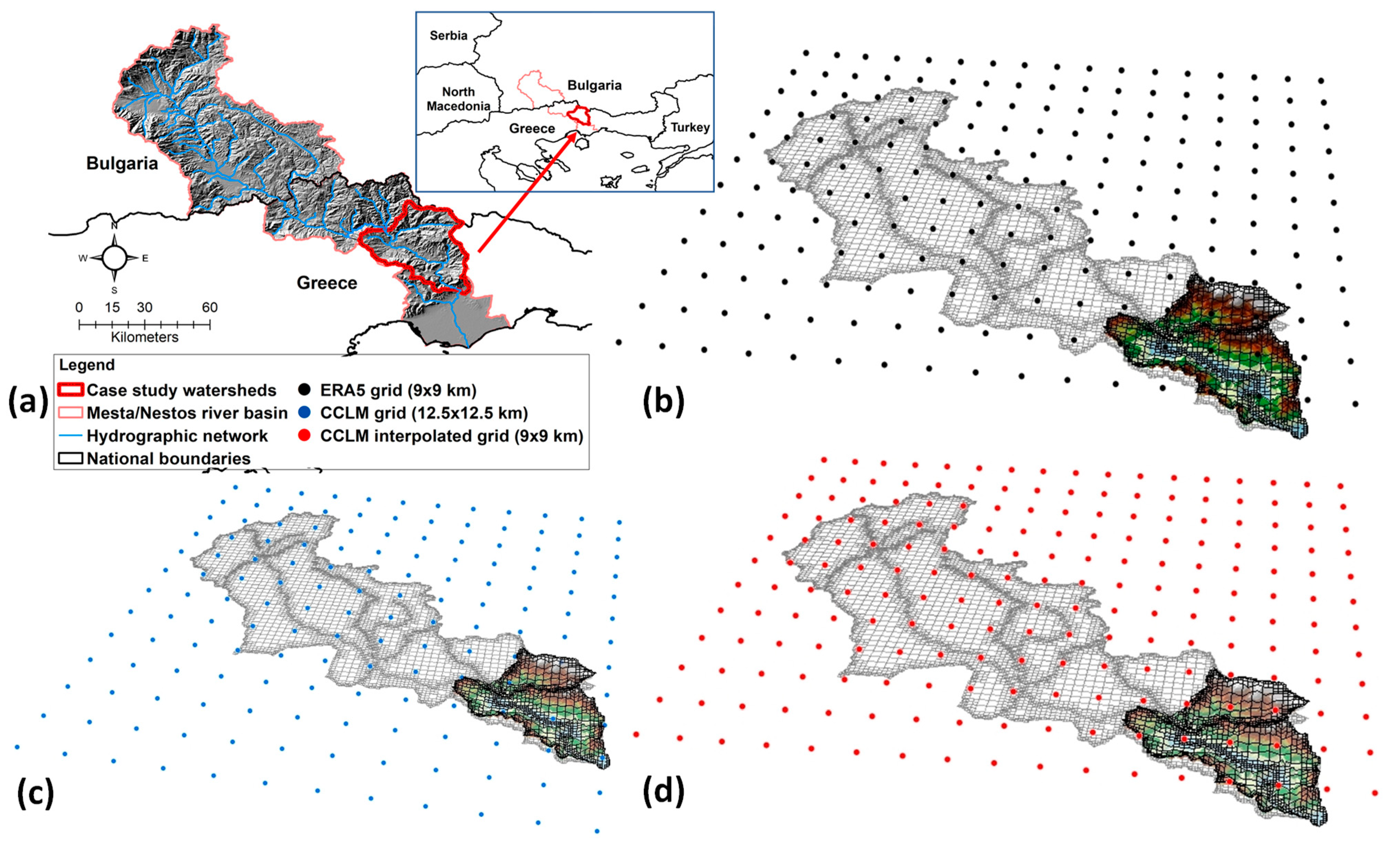
2.1. Case Study Area

The case study area consists of selected neighboring watersheds at the Greek part of the Mesta/Nestos transboundary river basin that is shared between Bulgaria and Greece, Figure 1a. The case area is a mountainous one with a mean elevation of 981.0 m above sea level and an extent of 1235 km², i.e., it covers 41.6% of the Greek part of the basin. The waters of these watersheds are drained in the river’s main course and together with the upstream waters, which are released from existing hydropower plants, are accumulated to the lower deltaic area for covering the irrigation demands and preserving the identified important ecosystems [46].

The selection of the specific area is based on two facts. Firstly, it is a natural one, i.e., no mankind interventions have been ever implemented within its area, as well as the local population of 6141 inhabitants is concentrated in 44 small settlements [46]. The nonexistence of large-scale hydraulic projects secures the hydrological simulation of the selected hydrosystem from uncertainties coming from the operation of such projects. Secondly, the specific area has particular research importance since the development of a new dam for controlling the watersheds waters in the near future is proposed in the Program of Measures of the River Basin Management Plan of the river [47]. Hence, the proposed methodology and outputs could shed light on the way that climate change assessments should be integrated in the planning of this new project.

2.2. Utilized Datasets, bias Correction, and Spatio-Temporal Methods

2.2.1. ERA5 Precipitation and Temperature

The daily precipitation and the temperature data used in this research as reference data derives from the ERA5-Land reanalysis products. ERA5-Land is the most recent public release of the fifth generation of atmospheric reanalysis data by the European Centre for Medium Range Weather Forecasts (ERA5) dataset and are provided by the Copernicus (https://cds.climate.copernicus.eu/cdsapp#!/dataset/reanalysis-era5-land?tab=overview accessed on 17 September 2021). ERA5-Land is an evolution of the land component of the ERA5 climate reanalysis, driven by meteorological fields from ERA5 [14]. ERA5-Land database comprises parameters at a global scale from 1979 to 2–3 months before to the present at a finer resolution of 9 × 9 km in comparison to the ERA5. The daily precipitation and temperature dataset regarding this investigation covers the period from 1981 to 2000 with a spatial resolution of 9 × 9 km, Figure 1b.

2.2.2. Climate Model

The regional climate model CLMcom-ETH- COSMO-crCLIM-v1 (CCLM) forced by the general circulation model NVCC-NorESM-M and developed by the ETH Institute (Zurich) in collaboration with the limited-area modeling community (CLM community) [48,49] was used in this research. The climate model outputs regarding historical daily precipitation and temperature were downloaded from the CORDEX database (www.cordex.eu accessed on 5 May 2021). The spatial resolution of the climate model data corresponds to 12.5 × 12.5 km, Figure 1c, for the period 1981–2000.

2.2.3. Bias Correction Methods

In this research, the empirical quantile mapping (EQM) method was used, as it is an extended, efficient, and easily applicable bias correction technique concentrated on the entire distribution [50]. According to the EQM method the simulated values are calibrated by the reference ones using their cumulative distribution functions (CDF). It can be described by the following mathematical function (Equation (1)) [51]

$$x_0=F_0^{-1}\left(F_m\left(x_m\right)\right),$$

(1)

where $x_0$ the observed variable, $x_m$ the modeled variable, $F_0^{-1}$ the CDF of $x_m$, and $F_m$ the inverse CDF corresponding to $x_0$.

The solution of the equation is accomplished by using theoretical distributions. Piani et al. [52] and Cannon [53] assume that the F transfer function is a mixture of the Bernoulli and the Gamma distribution. In particular, the Bernoulli distribution is used to simulate the probability of precipitation occurrence and the Gamma distribution utilized to model precipitation. The normal distribution is used for the temperature data [54].

The proposed bias correction method was implemented into the historical CCLM climate model outputs. The evaluation of the EQS method was based on a cross-validation procedure with two 10-year sub-periods. The first sub-period from 1981 to 1990 was used to calibrate the method and the formulation considered in the research was applied with the climate4R tools [55,56,57]. It should be mentioned that in this study the transfer function differs from grid to grid and it depends on the precipitation and temperature data of each studied point. The Bernoulli, Gamma, Bernoulli–Weibull, Bernoulli–log-normal, Bernoulli–exponential, and normal distributions [58] are assessed. The bias correction is only applied on rainy days (>0.1 mm) for the parameter of precipitation and for the entire dataset of temperature. The data from the subperiod from 1991 to 2000 were used for validation purposes against the reference ERA5 precipitation and temperature data. The same EQM method was also implemented to the CCLM outputs that were initially spatially interpolated.

2.2.4. Spatio-Temporal Kriging Method

The spatio-temporal kriging was used to provide high resolution climate data for the hydrological simulation. All datasets were re-gridded to the ERA5-Land spatial resolution (9 × 9 km). The spatio-temporal kriging using the sum-metric covariance model [41] was implemented to: (1) the raw historical CCLM climate data and (2) the bias corrected CCLM climate model data. In Venetsanou et al.’s [41] research, the spatio-temporal kriging was applied by using five covariance models (separable, product-sum, metric, sum-metric, simple sum-metric covariance model) into a general circulation model’s output. The derived results were assessed compared to the ERA-Interim reanalysis precipitation and temperature and indicated that the sum-metric spatio-temporal covariance model is the most reliable spatio-temporal covariance model.

Gräler et al. [59] and Pebesma and Gräler [60] analytically describe the spatio-temporal process. Detailed information about the sum-metric covariance model and its spatio-temporal variogram are given by Bilonick [61] and Snepvangers et al. [62] with the formulas attributing the sum-metric covariance model (Equation (2)) and its variogram (Equation (3)) to be as

$$C_{sm}\left(h,u\right)=C_s\left(h\right)+C_t\left(u\right)p-+C_j\left(\sqrt{h^2+{(k\times u)}^2}\right),$$

(2)

$${\gamma }_{sm}\left(h,u\right)={\gamma }_s\left(h\right)+{\gamma }_t\left(u\right)+{\gamma }_j\left(\sqrt{h^2+{(k\times u)}^2}\right),$$

(3)

where γ_s, γ_t and γ_j are spatial, temporal, and joint variograms with a separate nugget-effect.

The krigeST function was utilized for the spatio-temporal kriging application [59,60,63]. The WGS84 coordinate reference system was used. The theoretical variogram for the climate data, with a spatial resolution of 12.5 × 12.5 km, was modeled and used as an input for the fitting routines of the sum-metric covariance model. The sample variogram was estimated by the vgmST, function with time lags of 1 day and spatial lags of 0.2 degrees.

To sum up, in this research the ERA5-Land datasets (hereinafter indicated as ERA5) regarding precipitation and temperature are considered as the reference datasets. The climate change model’s raw data are taken as the second set of data (hereinafter mentioned as CCLM), the bias corrected climate change data form the third utilized dataset (hereinafter denoted as CCLM_BC), the fourth set of data are the bias corrected and then spatiotemporally interpolated over the case study area CCLM data (hereinafter noted as CCLM_BC_SPK), and finally the data derived by the spatio-temporal interpolation followed by the bias correction of the CCLM model’s data (hereinafter mentioned as CCLM_SPK_BC) is the fifth dataset. It should be mentioned that the CCLM_BC dataset was used only within the hydrological modeling process to indicate the biases produced in simulated discharges when unbiased climate data are used.

Table 1. Definition of the abbreviations used in the research.

Abbreviation	Definition
ERA5	ERA5-Land dataset
CCLM	CLMcom-ETH-COSMO-crCLIM_v1 climate model outputs
CCLM_BC	Empirical quantile mapping bias correction on CCLM climate data
CCLM_BC_SPK	Empirical quantile mapping bias correction on CCLM climate data followed by spatio-temporal kriging
CCLM_SPK_BC	Spatio-temporal kriging on CCLM climate outputs followed by bias correction with the empirical quantile mapping method

gives the synopsis of the utilized abbreviations and their sort descriptions.

2.3. Hydrological Modeling

The hydrological simulation of the selected watersheds was conducted with a spatial distributed hydrology model, namely MODSUR (MODelisation du SURface) [64]; a model that has routinely been used for the simulation of the Mesta/Nestos river basin [32,46]. A thorough description of the models’ equations and structure is given in Skoulikaris et al. [65]. Briefly, by allocating daily precipitation, temperature, and potential evapotranspiration data series over the grid representing a case study river basin, the model repartitions rainfall into runoff, infiltration, and evapotranspiration at each grid’s cell and the accumulated runoff is finally computed in those grid’s cells that correspond to the river’s network at daily time step. In the research, the calibrated and validated version of the MODSUR model over the Mesta/Nestos river basin, based on gauged meteorological data and measured discharges from 1987 to 1995 (coefficient of determination (R²) = 0.69) [66], was adopted for the simulation of the case study area. The capability of the same model’s version to adequately simulate the river runoff (R² = 0.68) was also verified when ERA-Interim atmospheric reanalysis datasets from 1981 to 1995 and of varying spatial resolutions (0.50° × 0.50°, 0.25° × 0.25°, and 0.125° × 0.125°) were used as forcings [65]. Hence, in the utilized MODSUR model version all physical based parameters (e.g., land uses, topographic characteristics) and customized parameterizations (e.g., infiltration coefficients) embedded in the model’s grid, consisting of 9219 cells, are kept the same as in the research of Skoulikaris et al. [65]. Thereafter, the simulated river discharges are produced by forcing the model with daily precipitation, temperature, and evapotranspiration data series coming from the (a) ERA5, (b) CCLM, (c) CCLM_BC, (d) CCLM_BC_SPK, and (e) CCLM_SPK_BC datasets, with the ERA5 runoff to be considered the reference one.

At this point, it should be mentioned that the input datasets only included precipitation and temperature data, thus the evapotranspiration per dataset was calculated according to the adjusted Thornthwaite formula and to the conversion of monthly outputs to daily time series as given in the research of Sepaskhah and Razzaghi [67]. Moreover, although the case study area consists of 1870 grid’s cells, its simulation was based on the grid covering the whole Mesta/Nestos basin coming from the validated version of the MODSUR model. The reason behind this was to avoid producing any unexpected biases over the validated model during the hydrological simulation process. For that purpose, the input variables (precipitation, temperature, evapotranspiration) regarding the grid’s cells that do not belong to the case study area were artificially set to zero, while the input datasets corresponding to the case study area were properly nested within the model’s grid with the use of geographic information systems.

3. Results

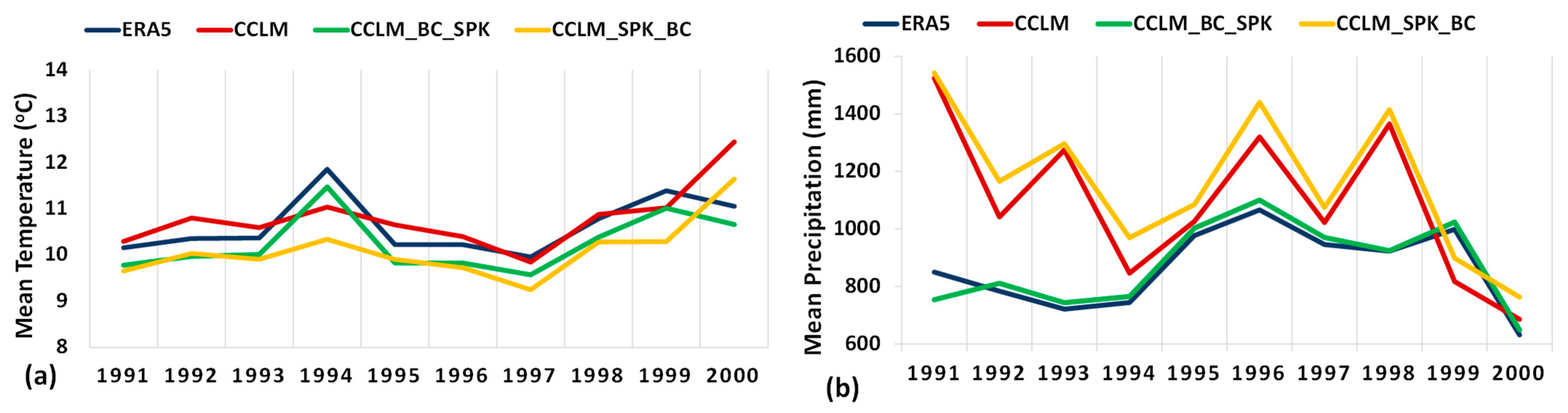
3.1. Climate Datasets Analysis’ Outputs

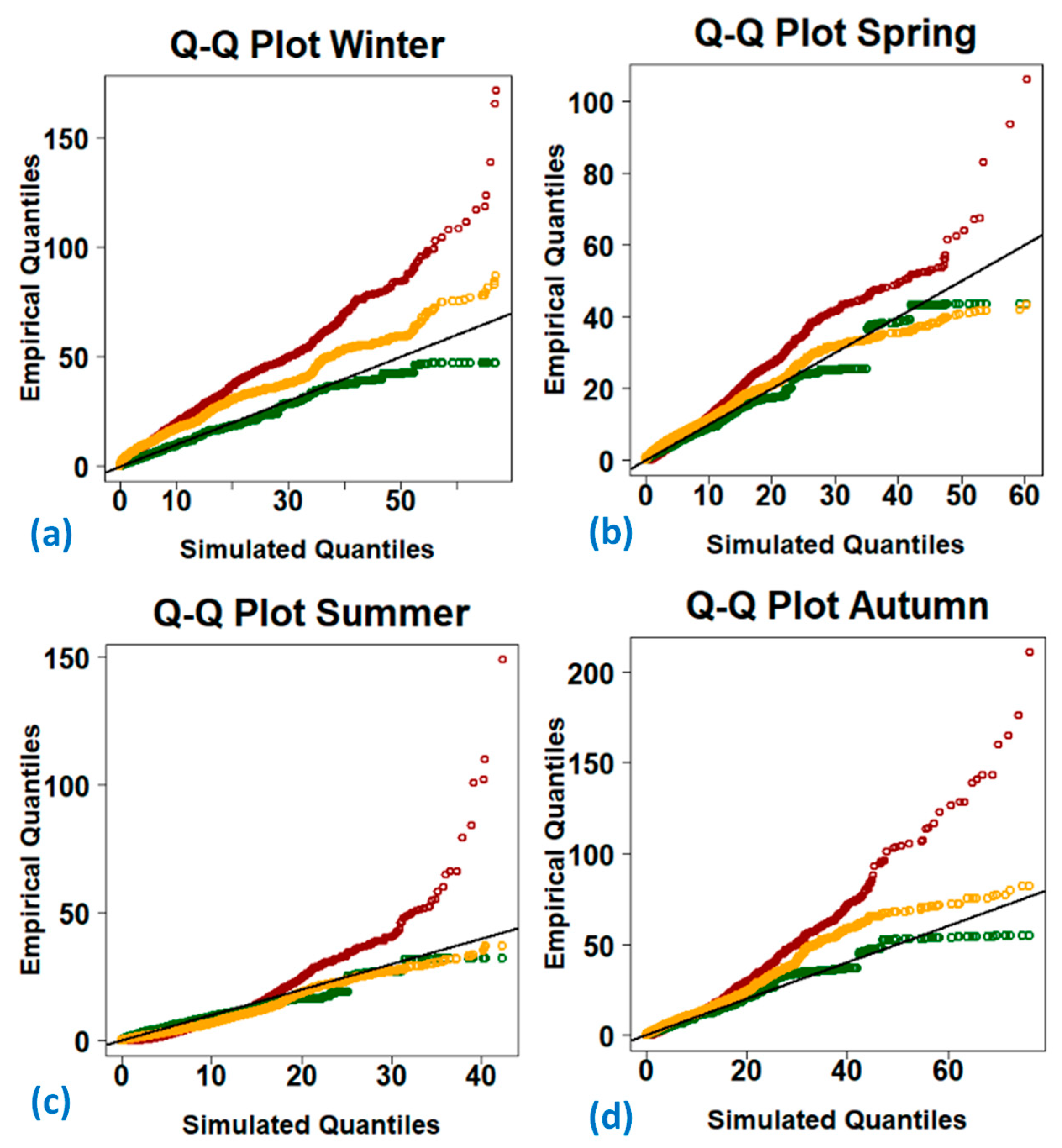
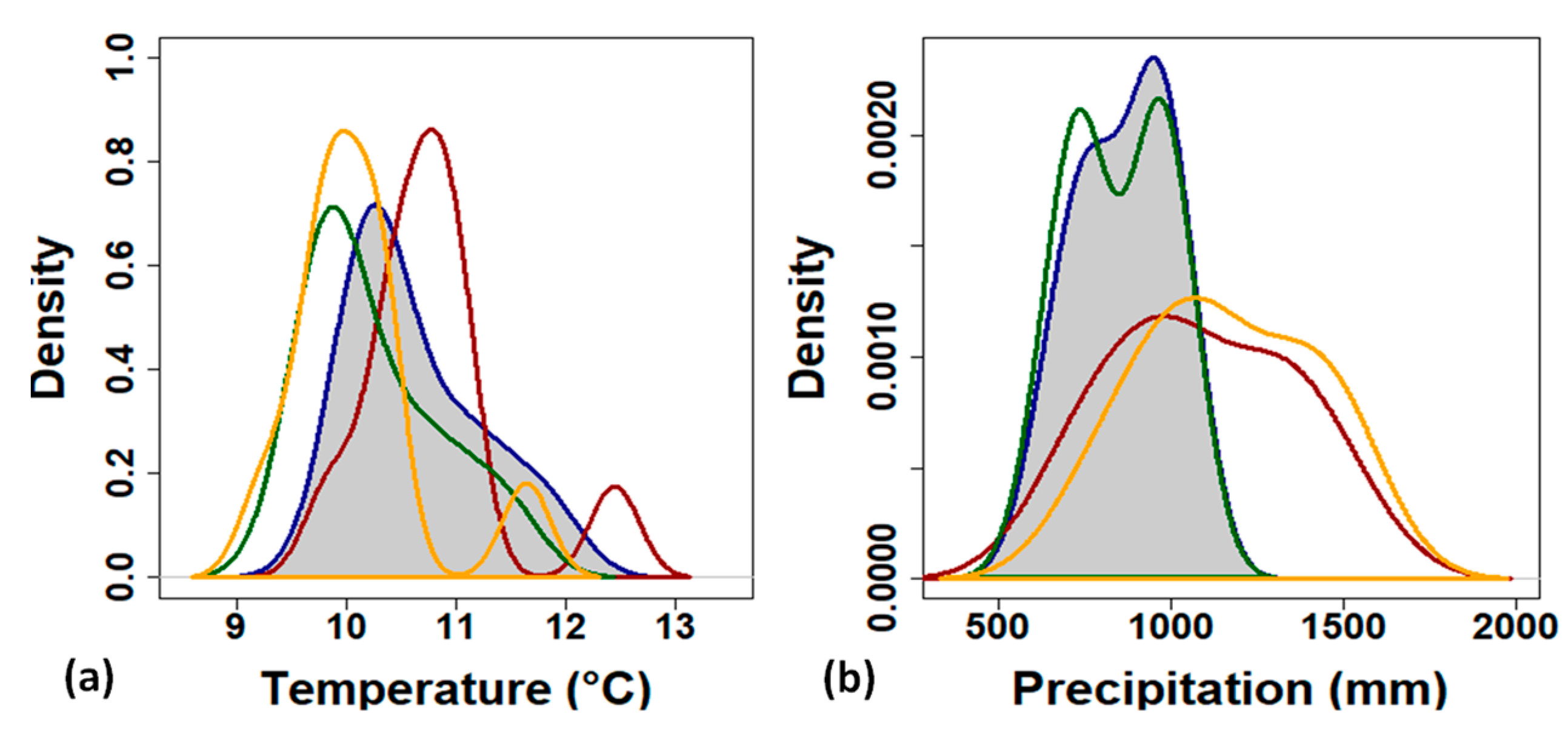
3.1.1. Precipitation Data

The analysis of the precipitation datasets at interannual level for the period 1991–2000 showed that the mean precipitation of the ERA5 and CCLM data is 864 mm and 1092 mm respectively, Figure 2b. Applying the combinations of the proposed bias correction and spatio-temporal kriging interpolation method, the mean annual precipitation of the CCLM_BC_SPK dataset equals 874 mm (very close to the one of ERA5), while the CCLM_SPK_BC precipitation is 1165 mm, i.e., even higher than the precipitation in the raw CCLM dataset. The maximum annual precipitation of the ERA5 and CCLM dataset within the 10-year period is 1066 mm and 1523 mm respectively. In the case of CCLM_BC_SPK and CCLM_SPK_BC datasets, the maximum annual precipitation during the simulation period is 1100 mm and 1541 mm respectively, i.e., similar to the ERA5 and CCLM maxima respectively.

The precipitation’s seasonal Q-Q plots, i.e., the quantiles plots of the reference dataset (ERA5) against the quantiles of the other datasets (CCLM, CCLM_BC_SPK, and CCLM_SPK_BC), for the period of 1991 to 2000 are depicted in Figure 3. Comparing the ERA5 and CCLM precipitations, significant differences appear between the two datasets during all seasons, as the CCLM precipitation (red curves in Figure 3) diverges from the ERA5 one (black diagonal line in Figure 3). The greater deviations are detected during the winter (Figure 3a) and autumn (Figure 3d) periods, meaning that the CCLM’s simulated precipitation overestimated the respect ERA5′s precipitation. This overestimation is lower during the spring (Figure 3b) and summer (Figure 3c) periods.

The application of the spatio-temporal kriging on the empirical quantile mapping bias corrected climate data (CCLM_BC_SPK) radically increased the accuracy of the climate data. The CCLM_BC_SPK precipitation attributed by the green curves of Figure 3 approaches the reference precipitation—i.e., the black diagonal line—in all seasons, and the results for the lower and upper tail of the plot have been significantly improved. The convergence of the two dataset is recorded particularly in the winter (Figure 3a) and autumn (Figure 3d) periods. In contrast, in the case of the reverse methodology—i.e., the CCLM_SPK_BC data—the outcomes are less satisfactory. Based on the Q-Q plot, the CCLM_SPK_BC precipitation’s curve (green curve of Figure 3) deviates from the reference curve (black line of Figure 3).

The classification of the best method—i.e., CCLM_BC_SPK or CCLM_SPK_BC—is also established by the precipitation density plots, Figure 4b, where it is clearly depicted that the mean annual CCLM_BC_SPK curve fits better the distribution of ERA5, than the curve of CCLM_SPK_BC. In particular, the daily CCLM_BC_SPK and ERA5 precipitation differences are minimized for the period from 1991 to 2000 over the research area, while in the case of the CCLM and CCLM_SPK_BC an important overestimation of the precipitation is observed.

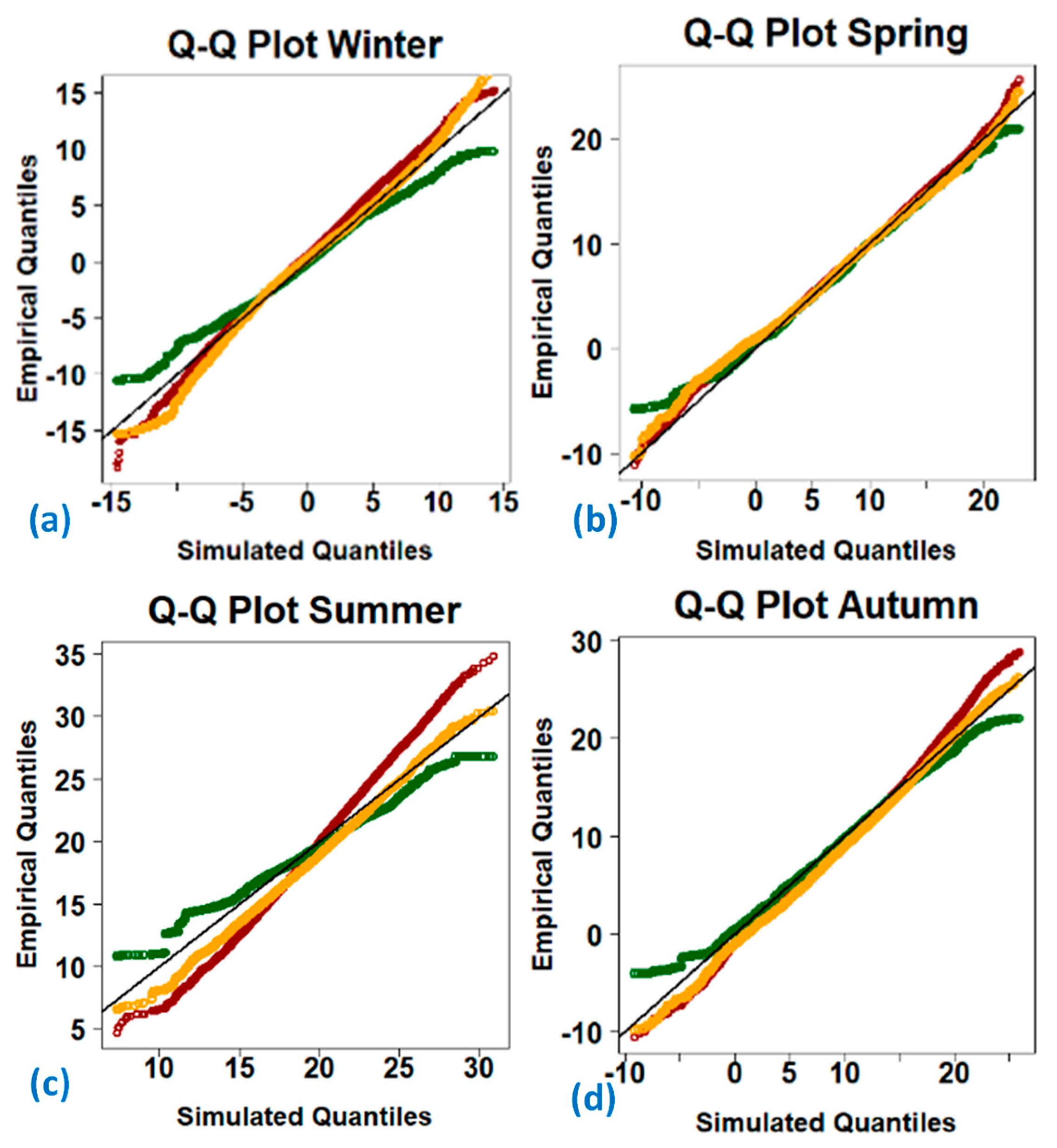
3.1.2. Temperature Data

In terms of mean interannual temperatures, ERA5 temperature is estimated at 10.6 °C, while CCLM, CCLM_BC_SPK, and CCLM_SPK_BC temperatures equal 10.9 °C, 10.3 °C, and 10.1 °C, respectively, Figure 2a, thus slight differences are presented among the different datasets at interannual level. At seasonal time step, the Q-Q plots of Figure 5 demonstrate the ERA5, CCLM, CCLM_BC_SPK, and CCLM_SPK_BC seasonal temperature for the period 1991–2000 and designate that the temperature present smaller biases in comparison to the precipitation. Biases occur in summer and autumn temperature, where the CCLM’s curve (red curve of Figure 5c,d respectively) diverge from the reference line (black line), especially in the upper tail of the plot. On the other hand, a clear convergence between the ERA5 and CCLM_BC_SPK and the ERA5 and CCLM_SPK datasets is observed in all seasonal graphs, meaning that in terms of temperature both CCLM_BC_SPK and CCLM_SPK data match the reference temperature. On the other hand, the temperature density plot, Figure 4a, suggests that the CCLM_SPK_BC data is close to the CCLM temperature and diverge from the ERA5 with the temperature being overestimated under the CCLM_SPK_BC method. Hence, it can be conceived that—at the climate variables level—the bias correction implementation followed by spatio-temporal kriging analysis (CCLM_BC_SPK) proves to be the more efficient methodology as it significantly improves the accuracy of the climate model outputs.

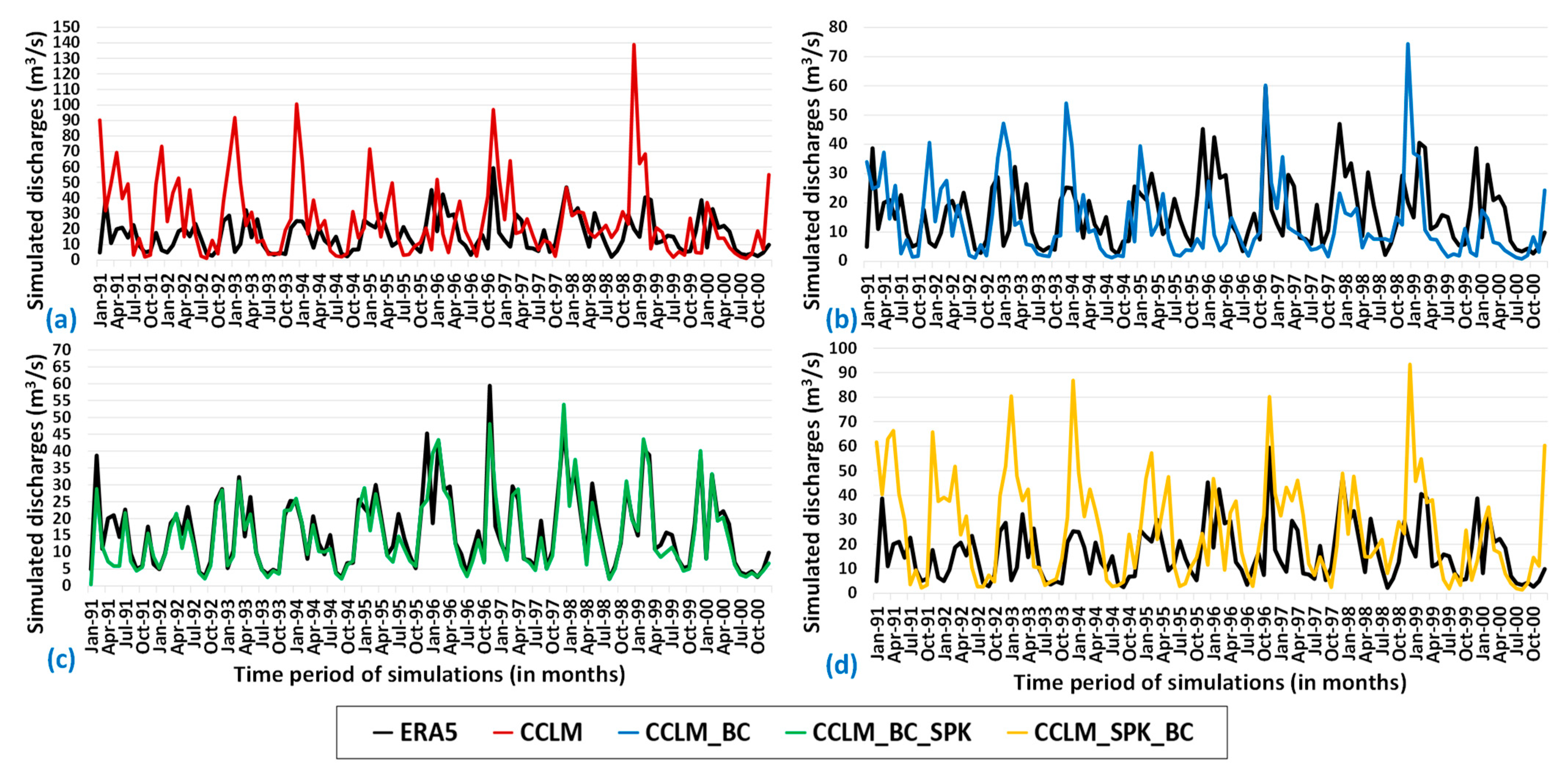
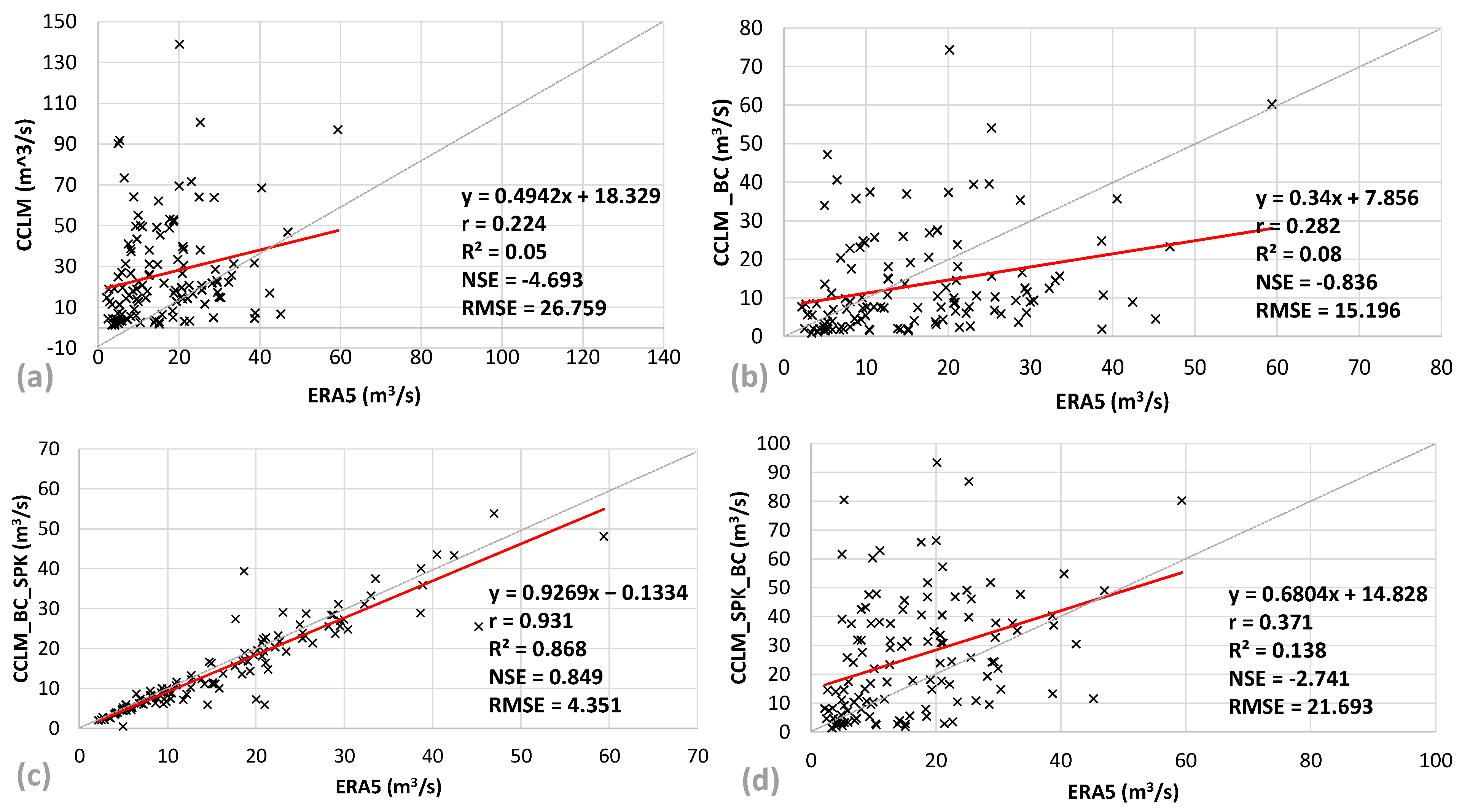
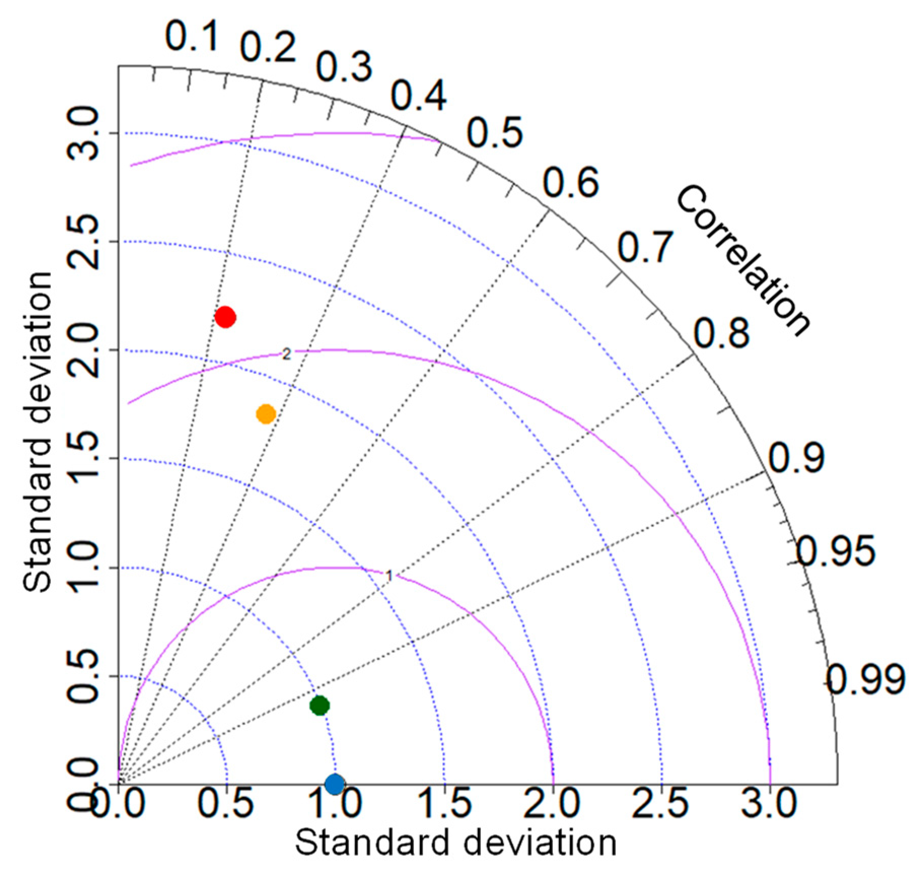
3.2. Hydrological Simulation Outputs

The simulation outputs when the hydrological model is forced by the ERA5 dataset demonstrate that the mean and maximum monthly river’s discharges (n = 120 months) at the basin’s outlet are 16.28 m³/s and 59.38 m³/s respectively, Figure 6. In case of forcing by the CCLM dataset, the mean river’s runoff equals 26.38 m³/s, i.e., 38.28% more than the reference runoff, and the maximum runoff equals 138.86 m³/s, i.e., 57.24% more than the reference one, Figure 6a. The hydrological model triggered by the bias corrected climate model dataset, i.e., the CCLM_BC dataset, shows that the mean and maximum runoff equal 13.39 m³/s (21.58% less than the reference one) and 74.34 m³/s (20.12% more than the reference maximum discharges) respectively, Figure 6b. When the climate model’s biased corrected and spatiotemporally interpolated data—i.e., the CCLM_BC_SPK data—are used, the mean intermontly discharges are 14.96 m³/s (8.8% less than the reference runoff) while the maximum equals 53.84 m³/s (10.2% less than the reference maximum), Figure 6c. Finally, when the forcing of the hydrological model is conducted by the climate model’s spatiotemporally interpolated and bias corrected dataset, i.e., the CCLM_SPK_BC dataset, the mean discharges are 25.90 m³/s (37.14% more than the reference ones) and the maximum discharges are 93.39 m³/s (36.41% more than the reference maximum), Figure 6d.

As presented in the discharges time series analysis and the graphs of Figure 6, the correlation analysis between the ERA5 reference runoff and the runoff coming from forcing of the hydrological model by the (a) CCLM, (b) CCLM_BC, (c) CCLM_BC_SPK, and (d) CCLM_SPK_BC datasets, Figure 7, establishes that the discharges attributed to the biased corrected and then spatiotemporally interpolated climate change data, i.e., to the CCLM_BC_SPK dataset, have the higher degree of correlation with the reference runoff. Particularly, as indicated by the utilized statistical performance measures and relevant scatter plots, the correlation between the ERA5 and CCLM derived discharges is low (Pearson correlation coefficient (r) = 0.224, coefficient of determination (R²) = 0.05, Nash–Sutcliffe efficiency coefficient (NSE) = −4.693, and root mean square error (RMSE) = 26.759), Figure 7a. The bias correction of the CCLM data demonstrates a slight amelioration of the correlation between the ERA5 and CCLM_BC derived discharges (r = 0.282, R² = 0.08, NSE = −0.836, RMSE = 15.196), Figure 7b. In the case of the CCLM_BC_SPK dataset, i.e., when the bias correction of the climate model’s variables is followed by spatio-temporal kriging interpolation, the ERA5 and CCLM_BC_SPK discharges are highly correlated (r = 0.931, R² = 0.868, NSE = 0.849, RMSE = 4.351) as explicitly depicted in Figure 7c. On the other hand, the reverse process—i.e., the climate model’s variables spatio-temporal kriging interpolation followed by the bias correction, as attributed in the CCLM_SPK_BC dataset—shows a relatively low correlation between the ERA5 and CCLM_SPK_BC discharges (r = 0.371, R² = 0.138, NSE = −2.741, RMSE = 21.693), Figure 7d.

The classification of the CCLM_BC_SPK as the best performance method regarding the discharges is also confirmed by the Taylor diagram of Figure 8, where the r, NSE, and RMSE are demonstrated simultaneously for all the simulated data. The Taylor diagrams [68] illustrate a statistical summary of how closely the simulated dataset approaches the reference data, with the standard deviation to be demonstrated by the radial distances from the reference point to sample, the correlation coefficient between the two fields by the azimuthal positions, and the root-mean-square difference to be given by the semicircles. Overall, in our case study the runoff linked with the CCLM_BC_SK dataset (green dot) is the closest one to the reference ERA5 discharge data (blue dot), having the highest correlation coefficient and the smaller standard deviation which results in the small RMS error. The figures corresponding to the r, NSE, and RMSE of each method represented by the colored dots in Figure 8 are the same with the ones presented within the Figure 7.

4. Discussion

The research presents a methodological analysis of the order of processes that ought to be performed before using gridded climate change data in surface hydrological modeling. The hierarchization of these processes—i.e., bias correction of gridded datasets followed by resolution downscaling through spatio-temporal interpolation or vice-versa—is not only investigated at a climate variable level, but is also examined and validated through runoff simulation comparisons at a case study river basin scale. The literature demonstrates a small number of scholars mainly focused on the climate variables level, such as the research of Rabiei and Haberlandt [45] that concluded that the merging of rain gauge and radar data through interpolation techniques (conditional merging and kriging with external drift) is ameliorated when the radar data are initially biased corrected, or Sharma et al. [69] who demonstrated that precipitation from global climate models (GCMs) need to be bias corrected and then spatially disaggregated before being used in hydrological simulation. However, a comparative analysis on which process needs to be first implemented in climate impacts assessment on water resources is rather limited.

4.1. Accuracy of Data, Methods, and Models

Although ERA5-Land is a new released product of current climatic variables, its utilization as reference data is justified by the numerous studies indicating their accuracy and applicability. Chiaravalloti et al. [70] used the ERA5-Land for the precipitation spatial distribution analysis over Italy, while Gleixner et al. [71] show that the annual cycle of the precipitation over the East Africa is well represented by the ERA5, diminishing the discrepancies during the rainy season. Tarek et al. [72] demonstrate the reduction of the ERA5 temperature and precipitation biases against the ERA-Interim product. Based on their findings, the hydrological simulation, using as input forcing data the ERA5 precipitation, provides similar results with the observed ones over North America. In an additional recent research, Xu et al. [73] compared, amongst other, the ERA5-Land precipitation with gauged data over China from 2016 to 2019 and concluded that the advantages of this product are its long time span, high spatial resolution, and relatively high temporal resolution, while the high latency of the data is mentioned as its weakness.

Regarding the selected bias correction method—i.e., the empirical quantile mapping (EQM) method—the literature proclaims the specific method for its high performance. Mendez et al. [74] compared six bias correction methods on adjusting the biases of historical monthly precipitation outputs from five GCMs dynamically downscaled by two RCMs for a total of seven different GCM-RCM pairs over Costa Rica and concluded that EQM marginally outperforms to the other methods. Similarly, Acharya et al. [75] indicated that the standardized-reconstruction and the quantile mapping method display the smallest RMSE in predicting rainfall series in an Indian monsoon area. A study focused on the alterations regarding the climate change signal (CCS) due to bias corrections induced by the quantile mapping method in an Italian case study [76] demonstrated that CCS is mainly altered for the temperature variable, since a CCS of the median ~ 1 °C lower than the original (~ 4.5 °C) is produced, while original CCS is essentially preserved for the precipitation. Although not implemented in this research, Mishra et al. [77] propose a very innovative approach for flood simulations under climate change, where the EQM method is implemented to bias correct the precipitation frequency, i.e., to convert days with scant precipitation to dry days so that the number of wet days from the GCM predictions to be approximately equal to actual observations. Moreover, the authors propose a threshold corresponding to the non-exceedance probability of observed zero precipitation so that the GCM precipitation intensities above the threshold value to be corrected according to the inverse of the CDF of GCM data with observation distribution parameters.

As far as the spatio-temporal kriging interpolation method is concerned, the method performance is demonstrated by Venetsanou et al. [41] where they present that the spatio-temporal kriging produces reasonable climate data for a Mediterranean river basin. Based on their outcomes, the MPI and HadGME2 climate change precipitation improved by 14% and 20%, respectively, satisfactorily approaching the ERA-Interim precipitation. Significant improvement was also observed in HadGME2 temperature. Heuvelink et al. [38] compared the spatio-temporal kriging with the regression kriging and concluded that it presents the lowest RMSE. Kilibrada et al. [78] applied the same method for the prediction of the mean, maximum, and minimum daily temperature at global scale.

As for the MODSUR hydrological model, the model has successfully been implemented in the past in the Mesta/Nestos basin for different gridded datasets such as the ERA-Interim products [32], different RCM models and scenarios [46], and various climatic scenarios from the Fourth Assessment Report (AR4), e.g., A1B and B1 [66]. The specific model has also been applied on river basins of varying scales, e.g., in the Maritza river basin in Bulgaria [79], and in the Seine [80] and Rhône [81] river basins in France. Finally, the CLMcom-ETH-COSMO-crCLIM_v1 regional climate model (mentioned as CCLM) used in the research is under the auspices of the Coordinated Regional Climate Downscaling Experiment (CORDEX), an issue that demonstrated its validated applicability on a European scale [49].

4.2. Interpretation of Findings

At precipitation and temperature variables level, the simulation outputs demonstrated that the CCLM_BC_SPK method, i.e., Empirical Quantile Mapping bias correction of the CLMcom-ETH-COSMO-crCLIM_v1 regional climate model data of 12.5 × 12.5 km resolution followed by the data spatio-temporal kriging interpolation at the resolution of 9 × 9 km, which is the spatial resolution of the ERA5 dataset, is the superior approach in comparison to the reverse CCLM_SPK_ BC method, i.e., the spatio-temporal kriging interpolation of the regional climate model data from 12.5 × 12.5 km to 9 × 9 km followed by the EQM bias correction of the produced data. The statistical evaluation conducted through the Q-Q (Figure 3 and Figure 5) and density (Figure 4) plots confirms that CCLM_BC_SPK dataset is well correlated with the reference ERA5 data in all seasons than the CCLM_SPK_BC does. The latter means that the CCLM_BC_SPK method leads to the optimization of the CCLM precipitation and temperature simulations over the study area.

As regards to precipitation data, with the CCLM_BC_SPK method the major improvement occurs during the winter (Figure 3a) and autumn (Figure 3d) periods. It is calculated that the biases are minimized by approximately 30% for the period from 1991 to 2000 and are properly adjusted on the ERA5 precipitation data. On the other hand, the application of the CCLM_BC_SPK method shows that although there is a significant decrease of the precipitation biases for the spring (Figure 3b) and summer period (Figure 3c), the specific method cannot converge the CCLM biases observed during the winter period (Figure 3a). Concerning the temperature, the CCLM temperature is close to the reference one, thus both the CCLM_BC_SPK and CCLM_SPK_BC simulated temperatures match the respective ERA5 precipitation for the corresponding period quite satisfactorily. In general, the outputs coincide with the research of Vautard et al. [49], where in the performed evaluation of the CCLM model, as part of the Euro-Cordex RCMs evaluation, they designate that, for the Mediterranean Basin, the specific RCM shows precipitation positive biases, thus the implementation of bias correction and spatial rectification methods are necessitated.

The outperformance of the CCLM_BC_SPK against the CCLM_SPK_BC method is proved to be established due to the order of implemented processes, particularly for the precipitation variable. In CCLM_BC_SPK, the initial bias correction of the CCLM precipitation results on an unbiased version of the CCLM grid nodes (with an average bias decrease over the case study of approximately 16–18%). Hence, the spatio-temporal kriging downscaling method, which is based on calculations of the sum-metric covariance and its variogram with the neighboring nodes, is conducted on unbiased grid’s nodes and produces an extra bias’ decrease of 12–14%, resulting on a total bias minimization of approximately 30%. On the other hand, when the spatio-temporal kriging interpolation method on the unbiased CCLM data is initially performed, the outcomes are simulated based on the surrounding grid points, which in this case are nodes with raw, i.e., biased, data. Thus, and since the raw data significantly differ from the ERA5 reference dataset, the downscaled new grid integrates the CCLM initial biases plus the ones coming from the spatio-temporal kriging method. Although, implementation of the EQM method at a second stage decreases the biases, the CCLM_SPK_BC product is more biased than the CCLM_BC_SPK by approximately 11% in terms of precipitation, which is the main variable influencing the surface hydrological modeling.

At hydrological level, the discharges produced by triggering the MODSUR model by the various datasets coincides with the outputs of the climate variables analysis, i.e., the CCLM_BC_SPK method is outranked as the best one. Initially, the very low correlation (negative Nash–Sutcliffe efficiency coefficient and very high root mean square error) of the reference discharges and the one produced with the use of the raw CCLM data validates the necessity of using unbiased climate change data in hydrological simulation, an issue that is also clearly demonstrated in the literature [28]. Thereafter, the comparison of the runoff triggered by the ERA5 and the bias corrected CCLM data—i.e., CCLM_BC—demonstrate an amelioration of the biases (Nash–Sutcliffe efficiency coefficient around zero and around 40% amelioration of the RMSE in comparison with the raw data). The application of the spatio-temporal kriging on the CCLM_BC data—i.e., CCLM_BC_SPK dataset—resulted on an important improvement on the comparison metrics between the references and the simulated with this method discharges (r = 0.931, R² = 0.868, NSE = 0.849, RMSE = 4.351), as thoroughly demonstrated in Figure 7c. On the other hand, the CCLM_SPK_BC produced discharges when compared with the reference ones, Figure 7d, although demonstrating a moderate correlation, the outputs are definitely inferior to those of the CCLM_BC_SPK approach. The CCLM_SPK_BC discharges, nevertheless, appear to have less biases than the ones produced by solely implementing bias correction.

5. Conclusions

The importance of this paper comes from its methodological approach to generate quality fit-to-purpose climate data that can be used in hydrological simulations. The research demonstrates that climate-change impact assessment at river basin scales necessitates unbiased climate data at finer spatial scales. Moreover, it is established that when well-validated reanalysis products (in our case the ERA5 datasets) are used for bias correction and spatial downscaling of gridded climatic datasets, bias correction should be followed by spatio-temporal techniques to achieve the maximum correlation with the reference datasets.

At precipitation level, the bias correction of the climate change precipitation and then its spatio-temporal interpolation is proved to produce high accuracy outputs in relation to the reference precipitation. Additionally, the spatio-temporal interpolation component significantly ameliorates the derived outputs in comparison to just implementing bias correction. On the other hand, when initially applying the spatio-temporal interpolation on the climate change data, the produced spatially rectified gridded dataset integrates the biases of the climate data which, thereafter, are partially corrected by the implemented bias correction method. In terms of temperature, the limited biases between the reference and climate change datasets results on the successful convergence of both methods—i.e., bias correction followed by spatio-temporal interpolation and spatio-temporal interpolation trailed by bias correction—in ameliorating the raw data. Finally, at simulated discharges level, the results coincide with those of the precipitation analysis, and the simulated river discharges forced by bias corrected, and then spatially downscaled, datasets are remarkably correlated with the reference discharges.

Concluding, both gridded climate and climate change datasets covering large geographic areas are unique assets fostering, amongst others, water resources management under current and future conditions. Nevertheless, specific processes, as those implemented in the research, need to be applied to reduce the risk of considerable biases in hydrological simulations under climate change conditions. The proposed methodology is practically applicable in all hydrological climate-change impact studies where the reference and climate change datasets have different spatial resolutions.

References

1. Raimonet, M.; Oudin, L.; Thieu, V.; Silvestre, M.; Vautard, R.; Rabouille, C.; Moigne, P.L. Evaluation of Gridded Meteorological Datasets for Hydrological Modeling. J. Hydrometeorol. 2017, 18, 3027–3041. [Google Scholar] [CrossRef]
2. Fréjaville, T.; Benito Garzón, M. The EuMedClim database: Yearly climate data (1901–2014) of 1 km resolution grids for Europe and the Mediterranean Basin. Front. Ecol. Evol. 2018, 6, 31. [Google Scholar] [CrossRef] [Green Version]
3. Arshad, M.; Ma, X.; Yin, J.; Ullah, W.; Liu, M.; Ullah, I. Performance evaluation of ERA-5, JRA-55, MERRA-2, and CFS-2 reanalysis datasets, over diverse climate regions of Pakistan. Weather Clim. Extrem. 2021, 33, 100373. [Google Scholar] [CrossRef]
4. Xu, X.; Frey, S.K.; Boluwade, A.; Erler, A.R.; Khader, O.; Lapen, D.R.; Sudicky, E. Evaluation of variability among different precipitation products in the Northern Great Plains. J. Hydrol. Reg. Stud. 2019, 24, 100608. [Google Scholar] [CrossRef]
5. Dhanya, C.T.; Villarini, G. An investigation of predictability dynamics of temperature and precipitation in reanalysis datasets over the continental United States. Atmos. Res. 2017, 183, 341–350. [Google Scholar] [CrossRef]
6. Wong, J.S.; Razavi, S.; Bonsal, B.R.; Wheater, H.S.; Asong, Z.E. Inter-comparison of daily precipitation products for large-scale hydro-climatic applications over Canada. Hydrol. Earth Syst. Sci. 2017, 21, 2163–2185. [Google Scholar] [CrossRef] [Green Version]
7. Adler, R.F.; Huffman, G.J.; Chang, A.; Ferraro, R.; Xie, P.P.; Janowiak, J.; Rudolf, B.; Schneider, U.; Curtis, S.; Bolvin, D.; et al. The version-2 global precipitation climatology project (GPCP) monthly precipitation analysis (1979–present). J. Hydrometeorol. 2003, 4, 1147–1167. [Google Scholar] [CrossRef]
8. Kummerow, C.; Barnes, W.; Kozu, T.; Shiue, J.; Simpson, J. The tropical rainfall measuring mission (TRMM) sensor package. J. Atmos. Ocean. Technol. 1998, 15, 809–817. [Google Scholar] [CrossRef]
9. Kanamitsu, M.; Ebisuzaki, W.; Woollen, J.; Yang, S.-K.; Hnilo, J.J.; Fiorino, M.; Potter, G.L. NCEP–DOE AMIP-II Reanalysis (R-2). Bull. Am. Meteorol. Soc. 2002, 83, 1631–1644. [Google Scholar] [CrossRef]
10. Mesinger, F.; DiMego, G.; Kalnay, E.; Mitchell, K.; Shafran, P.C.; Ebisuzaki, W.; Jović, D.; Woollen, J.; Rogers, E.; Berbery, E.H.; et al. North American regional reanalysis. Bull. Am. Meteorol. Soc. 2006, 87, 343–360. [Google Scholar] [CrossRef] [Green Version]
11. Rienecker, M.M.; Suarez, M.J.; Gelaro, R.; Todling, R.; Bacmeister, J.; Liu, E.; Bosilovich, M.G.; Schubert, S.D.; Takacs, L.; Kim, G.-K.; et al. MERRA: NASA’s Modern-Era Retrospective Analysis for Research and Applications. J. Clim. 2011, 24, 3624–3648. [Google Scholar] [CrossRef]
12. Saha, S.; Moorthi, S.; Pan, H.L.; Wu, X.; Wang, J.; Nadiga, S.; Tripp, P.; Kistler, R.; Woollen, J.; Behringer, D.; et al. The NCEP climate forecast system reanalysis. Bull. Am. Meteorol. Soc. 2015, 91, 1015–1057. [Google Scholar] [CrossRef]
13. Dee, D.P.; Uppala, S.M.; Simmons, A.J.; Berrisford, P.; Poli, P.; Kobayashi, S.; Andrae, U.; Balmaseda, M.A.; Balsamo, G.; Bauer, P.; et al. The ERA-Interim reanalysis: Configuration and performance of the data assimilation system. Q. J. R. Meteorol. Soc. 2011, 137, 553–597. [Google Scholar] [CrossRef]
14. Hersbach, H.; Bell, B.; Berrisford, P.; Hirahara, S.; Horanyi, A.; Muñoz-Sabater, J.; Nicolas, J.; Peubey, C.; Radu, R.; Schepers, D.; et al. The ERA5 global reanalysis. Q. J. R. Meteorol. Soc. 2020, 146, 1999–2049. [Google Scholar] [CrossRef]
15. Pelosi, A.; Terribile, F.; D’Urso, G.; Chirico, G.B. Comparison of ERA5-Land and UERRA MESCAN-SURFEX Reanalysis Data with Spatially Interpolated Weather Observations for the Regional Assessment of Reference Evapotranspiration. Water 2020, 12, 1669. [Google Scholar] [CrossRef]
16. Hansen, J.; Ruedy, R.; Sato, M.; Lo, K. Global surface temperature change. Rev. Geophys. 2010, 48, RG4004. [Google Scholar] [CrossRef] [Green Version]
17. Jones, P.D.; Lister, D.H.; Osborn, T.J.; Harpham, C.; Salmon, M.; Morice, C.P. Hemispheric and large-scale land-surface air temperature variations: An extensive revision and an update to 2010. J. Geophys. Res. Atmos. 2012, 117, D05127. [Google Scholar] [CrossRef] [Green Version]
18. Hofstra, N.; Haylock, M.; New, M.; Jones, P.; Frei, C. Comparison of six methods for the interpolation of daily, European climate data. J. Geophys. Res.-Atmos. 2008, 113, D21110. [Google Scholar] [CrossRef] [Green Version]
19. Mavromatis, T.; Voulanas, D. Evaluating ERA-Interim, Agri4Cast, and E-OBS gridded products in reproducing spatiotemporal characteristics of precipitation and drought over a data poor region: The Case of Greece. Int. J. Climatol. 2021, 41, 2118–2136. [Google Scholar] [CrossRef]
20. Bosilovich, M.G.; Kennedy, J.; Dee, D.; Allan, R.; O’Neill, A. On the reprocessing and reanalysis of observations for climate. In Climate Science for Serving Society; Asrar, G.R., Hurrell, J.W., Eds.; Springer: Dordrecht, The Netherlands, 2013; pp. 51–72. [Google Scholar]
21. Krysanova, V.; Donnelly, C.; Gelfan, A.; Gerten, D.; Arheimer, B.; Hattermann, F.; Kundzewicz, Z.W. How the performance of hydrological models relates to credibility of projections under climate change. Hydrol. Sci. J. 2018, 63, 696–720. [Google Scholar] [CrossRef]
22. Hay, L.E.; Clark, M.P.; Wilby, R.; Gutowski, W.J.; Leavesley, G.H.; Pan, Z.; Arritt, R.W.; Takle, E.S. Use of Regional Climate Model Output for Hydrologic Simulations. J. Hydrometeorol. 2002, 3, 571–590. [Google Scholar] [CrossRef]
23. Kleinn, J.; Frei, C.; Gurtz, J.; Lüthi, D.; Vidale, P.L.; Schär, C. Hydrologic simulations in the Rhine basin driven by a regional climate model. J. Geophys. Res. D Atmos. 2005, 110, D04102. [Google Scholar] [CrossRef]
24. Johnson, F.; Sharma, A. Accounting for interannual variability: A comparison of options for water resources climate change impact assessments. Water Resour. Res. 2011, 47, W04508.I. [Google Scholar] [CrossRef]
25. Chen, J.; Brissette, F.P.; Chaumont, D.; Braun, M. Finding Appropriate Bias Correction Methods in Downscaling Precipitation for Hydrologic Impact Studies over North America. Water Resour. Res. 2013, 49, 4187–4205. [Google Scholar] [CrossRef]
26. Chen, C.; Haerter, J.O.; Hagemann, S.; Piani, C. On the contribution of statistical bias correction to the uncertainty in the projected hydrological cycle. Geophys. Res. Lett. 2011, 38, L20403. [Google Scholar] [CrossRef] [Green Version]
27. Teutschbein, C.; Seibert, J. Bias correction of regional climate model simulations for hydrological climate-change impact studies: Review and evaluation of different methods. J. Hydrol. 2012, 456, 12–29. [Google Scholar] [CrossRef]
28. Fujihara, Y.; Tanaka, K.; Watanabe, T.; Nagano, T.; Kojiri, T. Assessing the impacts of climate change on the water resources of the Seyhan River Basin in Turkey: Use of dynamically downscaled data for hydrologic simulations. J. Hydrol. 2008, 353, 33–48. [Google Scholar] [CrossRef]
29. Kidd, C.; Becker, A.; Huffman, G.; Muller, C.L.; Joe, P.; Skofronick-Jackson, G.; Kirschbaum, D. So, How Much of the Earth’s Surface Is Covered by Rain Gauges? Bull. Am. Meteorol. Soc. 2017, 98, 69–78. [Google Scholar] [CrossRef]
30. Fuka, D.R.; Walter, M.T.; MacAlister, C.; Degaetano, A.T.; Steenhuis, T.S.; Easton, Z.M. Using the Climate Forecast System Reanalysis as weather input data for watershed models. Hydrol. Process. 2014, 28, 5613–5623. [Google Scholar] [CrossRef]
31. Soriano, E.; Mediero, L.; Garijo, C. Selection of Bias Correction Methods to Assess the Impact of Climate Change on Flood Frequency Curves. Water 2019, 11, 2266. [Google Scholar] [CrossRef] [Green Version]
32. Lazoglou, G.; Anagnostopoulou, C.; Skoulikaris, C.; Tolika, K. Bias Correction of Climate Model’s Precipitation Using the Copula Method and Its Application in River Basin Simulation. Water 2019, 11, 600. [Google Scholar] [CrossRef] [Green Version]
33. Lagouvardos, K.; Kotroni, V.; Bezes, A.; Koletsis, I.; Kopania, T.; Lykoudis, S.; Mazarakis, N.; Papagiannaki, K.; Vougioukas, S. The automatic weather stations NOANN network of the National Observatory of Athens: Operation and database. Geosci. Data J. 2017, 4, 4–16. [Google Scholar] [CrossRef]
34. Liu, D.; Zhao, Q.; Fu, D.; Guo, S.; Liu, P.; Zeng, Y. Comparison of spatial interpolation methods for the estimation of precipitation patterns at different time scales to improve the accuracy of discharge simulations. Hydrol. Res. 2020, 51, 583–601. [Google Scholar] [CrossRef]
35. Cheng, M.; Wang, Y.; Engel, B.; Zhang, W.; Peng, H.; Chen, X.; Xia, H. Performance Assessment of Spatial Interpolation of Precipitation for Hydrological Process Simulation in the Three Gorges Basin. Water 2017, 9, 838. [Google Scholar] [CrossRef] [Green Version]
36. Teegavarapu, R.S.; Meskele, T.; Pathak, C.S. Geo-spatial grid-based transformations of precipitation estimates using spatial interpolation methods. Comput. Geosci. 2012, 40, 28–39. [Google Scholar] [CrossRef]
37. Yang, X.; Xie, X.; Liu, D.L.; Ji, F.; Wang, L. Spatial Interpolation of Daily Rainfall Data for Local Climate Impact Assessment over Greater Sydney Region. Adv. Meteorol. 2015, 2015, 563629. [Google Scholar] [CrossRef] [Green Version]
38. Heuvelink, G.B.; Griffith, D.A.; Hengl, T.; Melles, S.J. Sampling design optimization for space-time kriging. In Spatio-Temporal Design; John Wiley & Sons, Ltd.: Chichester, UK, 2012; pp. 207–230. ISBN 9781118441862. [Google Scholar]
39. Heuvelink, G.B.M.; Griffth, D.A. Space-time geostatistics for geography: A case study of radiation monitoring across parts of Germany. Geog. Anal. 2010, 42, 161–179. [Google Scholar] [CrossRef]
40. Gräler, B.; Rehr, M.; Gerharz, L.; Pebesma, E.J. Spatio-Temporal Analysis and Interpolation of PM10 Measurements in Europe for 2009. ETC/ACM Tech. Paper 2012/08 2013, 30p. Available online: https://www.eionet.europa.eu/etcs/etc-atni/products/etc-atni-reports/etcacm_2012_8_spatio-temp_pm10analyses (accessed on 4 January 2021).
41. Venetsanou, P.; Anagnostopoulou, C.; Loukas, A.; Lazoglou, G.; Voudouris, K. Minimizing the uncertainties of RCMs climate data by using spatio-temporal geostatistical modeling. Earth Sci. Inform. 2019, 12, 183–196. [Google Scholar]
42. Leta, O.T.; Nossent, J.; Velez, C.; Shrestha, N.K.; van Griensven, A.; Bauwens, W. Assessment of the different sources of uncertainty in a SWAT model of the River Senne (Belgium). Environ. Modell. Softw. 2015, 68, 129–146. [Google Scholar] [CrossRef]
43. Lobligeois, F.; Andréassian, V.; Perrin, C.; Tabary, P.; Loumagne, C. When does higher spatial resolution rainfall information improve streamflow simulation? An evaluation using 3620 flood events. Hydrol. Earth Syst. Sci. 2014, 18, 575–594. [Google Scholar] [CrossRef] [Green Version]
44. Sridharan, V.; Broad, O.; Shivakumar, A.; Howells, M.; Boehlert, B.; Groves, D.G.; Rogner, H.-H.; Taliotis, C.; Neumann, J.E.; Strzepek, K.M.; et al. Resilience of the Eastern African electricity sector to climate driven changes in hydropower generation. Nat. Commun. 2019, 10, 302. [Google Scholar] [CrossRef] [Green Version]
45. Rabiei, E.; Haberlandt, U. Applying bias correction for merging rain gauge and radar data. J. Hydrol. 2015, 522, 544–557. [Google Scholar] [CrossRef]
46. Skoulikaris, C.; Makris, C.; Katirtzidou, M.; Baltikas, V.; Krestenitis, Y. Assessing the vulnerability of a deltaic environment due to climate change impact on surface and coastal waters: The case of Nestos River (Greece). Environ. Mod. Assess. 2021, 26, 459–486. [Google Scholar] [CrossRef]
47. Special Secretariat for Water (SSW). The River Basin Management Plan of Thrace Water District (GR11); Ministry of Environment and Energy: Athens, Greece, 2013. (In Greek) [Google Scholar]
48. Pothapakula, P.K.; Primo, C.; Sørland, S.; Ahrens, B. The synergistic impact of ENSO and IOD on Indian summer monsoon rainfall in observations and climate simulations—An information theory perspective. Earth Syst. Dynam. 2020, 11, 903–923. [Google Scholar] [CrossRef]
49. Vautard, R.; Kadygrov, N.; Iles, C.; Boberg, F.; Buonomo, E.; Bülow, K.; Coppola, E.; Corre, L.; Meijgaard, E.; Nogherotto, R.; et al. Evaluation of the large EURO-CORDEX regional climate model ensemble. J. Geophys. Res. Atmos. 2020, 126, e2019JD032344. [Google Scholar] [CrossRef]
50. Panofsky, H.G.; Brier, G.W. Some Applications of Statistics to Meteorology; Mineral Industries Extension Services; College of Mineral Industries, Pennsylvania State University: State College, PA, USA, 1958. [Google Scholar]
51. Angus, J.E. The Probability Integral Transform and Related Results. SIAM Rev. 1994, 36, 652–654. [Google Scholar] [CrossRef]
52. Piani, C.; Haerter, J.O.; Coppola, E. Statistical bias correction for daily precipitation in regional climate models over Europe. Theor. Appl. Climatol. 2010, 99, 187–192. [Google Scholar] [CrossRef] [Green Version]
53. Cannon, A.J. Probabilistic Multisite Precipitation Downscaling by an Expanded Bernoulli Gamma Density Network. J. Hydrometeorol. 2008, 9, 1284–1300. [Google Scholar] [CrossRef]
54. Li, H.; Sheffield, J.; Wood, E.F. Bias correction of monthly precipitation and temperature fields from Intergovernmental Panel on Climate Change AR4 models using equidistant 15 quantile matching. J. Geophys. Res. 2010, 115, D10101. [Google Scholar] [CrossRef]
55. Casanueva, A.; Herrera, S.; Iturbide, M.; Lange, S.; Jury, M.; Dosio, A.; Maraun, D.; Gutiérrez, J.M. Testing bias adjustment methods for regional climate change applications under observational uncertainty and resolution mismatch. Atmos. Sci. Lett. 2020, 21, e978. [Google Scholar] [CrossRef] [Green Version]
56. Bedia, J.; Baño-Medina, J.; Legasa, M.N.; Iturbide, M.; Manzanas, R.; Herrera, S.; Casanueva, A.; San-Martín, D.; Cofiño, A.S.; Gutiérrez, J.M. Statistical downscaling with the downscaleR package (v3.1.0): Contribution to the VALUE intercomparison experiment. Geosci. Model Dev. 2020, 13, 1711–1735. [Google Scholar] [CrossRef] [Green Version]
57. Iturbide, M.; Bedia, J.; Herrera, S.; Baño-Medina, J.; Fernández, J.; Frías, M.D.; Manzanas, R.; San-Martínc, D.; Cimadevill, E.; Cofiño, A.S.; et al. The R-based climate4R open framework for reproducible climate data access and post-processing. Environ. Model. Softw. 2019, 111, 42–54. [Google Scholar] [CrossRef]
58. Cannon, A.J. Neural networks for probabilistic environmental prediction: Conditional Density Estimation Network Creation and Evaluation (CaDENCE) in R. Comput. Geosci. 2012, 41, 126–135. [Google Scholar] [CrossRef]
59. Gräler, B.; Gerharz, L.; Pebesma, E. Spatio-Temporal Interpolation using gstat. R J. 2016, 8, 204–218. [Google Scholar] [CrossRef]
60. Pebesma, E.; Graler, B. Introduction to Spatio-Temporal Variography; University of Münster: Münster, Germany, 2021. [Google Scholar]
61. Bilonick, R.A. Monthly hydrogen ion deposition maps for the northeastern U.S. from July 1982 to September 1984. Atmos. Environ. 1988, 22, 1909–1924. [Google Scholar] [CrossRef]
62. Snepvangers, J.; Heuvelink, G.; Huisman, J. Soil water content interpolation using spatio-temporal kriging with external drift. Geoderma 2003, 112, 253–271. [Google Scholar] [CrossRef]
63. Pebesma, E. spacetime: Spatio-Temporal Data in R. J. Stat. Softw. 2012, 51, 1–30. [Google Scholar] [CrossRef] [Green Version]
64. Ledoux, E.; Girard, G.; de Marsily, G.; Deschenes, J. Spatially distributed modelling: Conceptual approach, coupling surface water and ground water. In Unsaturated Flow Hydrologic Modelling-Theory and Practice; Morel-Seytoux, H.J., Ed.; NATO ASI Series S 275; Kluwer Academic: Boston, CA, USA, 1989; pp. 435–454. [Google Scholar]
65. Skoulikaris, C.; Anagnostopoulou, C.; Lazoglou, G. Hydrological Modeling Response to Climate Model Spatial Analysis of a South Eastern Europe International Basin. Climate 2020, 8, 1. [Google Scholar] [CrossRef] [Green Version]
66. Skoulikaris, C.; Ganoulis, J. Climate change impacts on river catchment hydrology using dynamic downscaling of global climate models. In National Security and Human Health Implications of Climate Change; Fernando, H.J.S., Klaic, Z.B., McCulley, J.L., Eds.; Springer: Dordrecht, The Netherlands, 2011; Volume 125, pp. 281–287. [Google Scholar]
67. Sepaskhah, A.R.; Razzaghi, F. Evaluation of the adjusted Thornthwaite and Hargreaves-Samani methods for estimation of daily evapotranspiration in a semi-arid region of Iran. Arch. Agron. Soil Sci. 2009, 55, 51–66. [Google Scholar] [CrossRef]
68. Taylor, K.E. Summarizing multiple aspects of model performance in a single diagram. J. Geophys. Res. 2001, 106, 7183–7192. [Google Scholar] [CrossRef]
69. Sharma, D.; Das Gupta, A.; Babel, M.S. Spatial disaggregation of bias-corrected GCM precipitation for improved hydrologic simulation: Ping River Basin, Thailand. Hydrol. Earth Syst. Sci. 2007, 11, 1373–1390. [Google Scholar] [CrossRef] [Green Version]
70. Chiaravalloti, F.; Caloiero, T.; Coscarelli, R. The Long-Term ERA5 Data Series for Trend Analysis of Rainfall in Italy. Hydrology 2022, 9, 18. [Google Scholar] [CrossRef]
71. Gleixner, S.; Demissie, T.; Diro, G.T. Did ERA5 Improve Temperature and Precipitation Reanalysis over East Africa? Atmosphere 2020, 11, 996. [Google Scholar] [CrossRef]
72. Tarek, M.; Brissette, F.; Arsenault, R. Evaluation of the ERA5 reanalysis as a potential reference dataset for hydrological modeling over North-America. Hydrol. Earth Syst. Sci. 2019, 10, 1009–1012. [Google Scholar]
73. Xu, J.; Ma, Z.; Yan, S.; Peng, J. Do ERA5 and ERA5-Land Precipitation Estimates Outperform Satellite-based Precipitation Products? A Comprehensive Comparison between State-of-the-art Model-based and Satellite-based Precipitation Products over Mainland China. J. Hydrol. 2022, 605, 127353. [Google Scholar] [CrossRef]
74. Mendez, M.; Maathuis, B.; Hein-Griggs, D.; Alvarado-Gamboa, L.-F. Performance Evaluation of Bias Correction Methods for Climate Change Monthly Precipitation Projections over Costa Rica. Water 2020, 12, 482. [Google Scholar] [CrossRef] [Green Version]
75. Acharya, N.; Chattopadhyay, S.; Mohanty, U.C.; Dash, S.K.; Sahoo, L.N. On the bias correction of general circulation model output for Indian summer monsoon. Meteorol. Appl. 2013, 20, 349–356. [Google Scholar] [CrossRef]
76. Sangelantoni, L.; Russo, A.; Gennaretti, F. Impact of bias correction and downscaling through quantile mapping on simulated climate change signal: A case study over Central Italy. Theor. Appl. Climatol. 2019, 135, 725–740. [Google Scholar] [CrossRef]
77. Mishra, B.K.; Rafiei Emam, A.; Masago, Y.; Kumar, P.; Regmi, R.K.; Fukushi, K. Assessment of Future Flood Inundations under Climate and Land Use Change Scenarios in the Ciliwung River Basin, Jakarta. J. Flood Risk Manag. 2018, 11, S1105–S1115. [Google Scholar] [CrossRef]
78. Kilibarda, M.; Hengl, T.; Heuvelink, G.B.M.; Gräler, B.; Pebesma, E.; Perčec Tadić, M.; Bajat, B. Spatio-temporal interpolation of daily temperatures for global land areas at 1 km resolution. J. Geophys. Res. Atmos. 2014, 119, 2294–2313. [Google Scholar] [CrossRef] [Green Version]
79. Artinyan, E.; Habets, F.; Noilhan, J.; Ledoux, E.; Dimitrov, D.; Martin, E.; Le Moigne, P. Modelling the water budget and the riverflows of the Maritsa basin in Bulgaria. Hydrol. Earth Syst. Sci. 2008, 12, 21–37. [Google Scholar] [CrossRef] [Green Version]
80. Rousset, F.; Habets, F.; Gomez, E.; Le Moigne, P.; Morel, S.; Noilhan, J.; Ledoux, E. Hydrometeorological modeling of the Seine basin using the SAFRAN-ISBA-MODCOU system. J. Geophys. Res. Atmos. 2004, 109, D14105. [Google Scholar] [CrossRef]
81. Quintana-Seguí, P.; Ribes, A.; Martin, E.; Habets, F.; Boé, J. Comparison of three downscaling methods in simulating the impact of climate change on the hydrology of Mediterranean basins. J. Hydrol. 2010, 383, 111–124. [Google Scholar] [CrossRef] [Green Version]
Figure 1. Illustration of (a) the Mesta/Nestos transboundary river basin and of the case study watersheds (red polygon), and of (b) the ERA5 grid (black dots) of 9 × 9 km resolution, (c) the CCLM grid of 12.5 × 12.5 km resolution (blue dots), and (d) the CCLM spatio-temporal interpolated grid (red dots) of 9 × 9 km resolution overlaying the hydrological model’s grid of the basin and of the case study area (represented by a 3D elevation model overlayed by the model’s grid).
Water 14 00660 g001
Figure 2. Mean annual variability of (a) temperature and (b) precipitation according to the ERA5 (black curve), CCLM (red curve), CCLM_BC_SPK (green curve), and CCLM_SPK_BC (orange curve) datasets for the period 1991–2000.
Water 14 00660 g002
Figure 3. Q-Q plots for the seasonal ((a) winter, (b) spring, (c) summer, (d) autumn) precipitation simulated for the ERA5 (black line), CCLM (red curve), CCLM_BC_SPK (green curve), and CCLM_SPK_BC (orange curve) datasets over the research area for the period 1991–2000.
Water 14 00660 g003
Figure 4. Density plots for the mean (a) temperature, and (b) precipitation computed for the ERA5 (blue curved grey area), CCLM (red curve), CCLM_BC_SPK (green curve), and CCLM_SPK_BC (orange curve) datasets over the research area for the period 1991–2000.
Water 14 00660 g004
Figure 5. Q−Q plots for the seasonal ((a) winter, (b) spring, (c) summer, (d) autumn) temperature simulated for the ERA5 (blue-black line), CCLM (red line), CCLM_BC_SPK (green line), and CCLM_SPK_BC (orange line) datasets over the research area for the period 1991–2000.
Water 14 00660 g005
Figure 6. Simulated runoff when the model is triggered by the ERA5 datasets (black curves) versus the runoff of (a) CCLM (red curve), (b) CCLM_BC (blue curve), (c) CCLM_BC_SPK (green curve), and (d) CCLM_SPK_BC (orange curve) forcings of the hydrological model.
Water 14 00660 g006
Figure 7. Correlation and statistical performance measures of the reference river’s discharges produced by forcing the hydrological model with the ERA5 dataset against the simulated discharges coming from forcing with (a) CCLM, (b) CCLM_BC, (c) CCLM_BC_SPK, and (d) CCLM_SPK_BC datasets respectively.
Water 14 00660 g007
Figure 8. Taylor diagram displaying a statistical comparison between the discharges forced by the reference ERA5 (blue dot), CCLM (red dot), CCLM_BC_SPK (green dot), and CCLM_SPK_BC (orange dot) data, with the black lines depicting the correlation coefficient, the purple curves depicting the centered RMS difference, and the blue curves indicating the standard deviation.
Water 14 00660 g008