On the Retrieval of the Water Quality Parameters from Sentinel-3/2 and Landsat-8 OLI in the Nile Delta’s Coastal and Inland Waters

Abstract

Reduced water quality due to the eutrophication process causes large economic losses worldwide. Multi-source remotely-sensed water quality monitoring can help provide effective water resource management. The research evaluates the retrieval of the water quality parameters: chlorophyll-a (Chl-a), total suspended matter (TSM), and chromophoric dissolved organic matter (CDOM), over optically different water types. Cross-sensor performance analysis of three satellite data sources: Sentinel-3 Ocean Land Color Imager (OLCI), Sentinel-2A Multi-Spectral Instrument (MSI), and Landsat-8 Operational Land Imager (OLI), acquired during a 45 min overpass on the Nile Delta coast on 22 March 2020 was performed. Atmospheric correction using the case 2 Regional Coast Color (C2RCC) was applied using local water temperature and salinity averages. Owing to the lack of ground-truth measurements in the coastal water, results were inter-compared with standard simultaneous color products of the Copernicus Marine Environment Monitoring Service (CMEMS), OLCI water full resolution (WFR), and the MODIS Aqua, in order to highlight the sensor data relative performance in the Nile Delta’s coastal and inland waters. Validation of estimates was carried out for the only cloud-free MSI data available in the 18–20 September 2020 period for the Burullus Lake nearly contemporaneous with in situ measurements in the 22–25 September 2020. Inter-comparison of the retrieved parameters showed good congruence and correlation among all data in the coastal water, while this comparison returned low positive or negative correlation in the inland lake waters. In the coastal water, all investigated sensors and reference data showed Chl-a content average of 3.14 mg m⁻³ with a range level of 0.39–4.81 mg m⁻³. TSM averaged 7.66 g m⁻³ in the range of 6.32–10.18 g m⁻³. CDOM clarified mean of 0.18 m⁻¹ in the range level of 0.13–0.30 m⁻¹. Analysis of the Mean Absolute Error (MAE) and the Root Mean Squared Error (RMSE) clarified that the MSI sensor was ranked first achieving the smallest MAE and RMSE for the Chl-a contents, while the EFR proved superior for TSM and CDOM estimates. Validation of results in Burullus Lake indicated a clear underestimation on average of 35.35% for the Chl-a induced by the land adjacency effect, shallow bottom depths, and the optical dominance of the TSM and the CDOM absorption intermixed in turbid water loaded with abundant green algae species and counts. The underestimation error increased at larger estimates of the algal composition/abundance (total counts, Chlorophyacea, Euglenophycaea, and Bacillariophycaea) and the biological contents (carbohydrates, lipids, and proteins), arranged in decreasing order. The largest normalized RMSE estimates marked the downstream areas where the inflow of polluted water persistently brings nutrient loads of nitrogen and phosphorous compounds as well as substantial amounts of detrital particles and sediments discharged from the agricultural and industrial drains and the land use changes related to agricultural practices, resulting in the increase of water turbidity giving rise to inaccurate Chl-a estimates.

1. Introduction

Coastal and inland water conditions, in particular, the chlorophyll-a (Chl-a) content and its accurate estimation controlling parameters, such as the total suspended matter (TSM) and the chromophoric dissolved organic matter (CDOM), are fundamental for effective monitoring of the water quality. Risk assessment of deteriorated water quality is vital to set preventive or ameliorative measures that can lead to better understanding and disclosing sources of contamination and anthropogenic effects, along with the prevailing eutrophication and climate change forces [1,2,3], which is a priority to the near shore communities who rely on such water resources. Eutrophication can lead to an increase in hypoxia, fish deaths, and the presence of harmful algae [2,4]. The Chl-a content is a proxy of the algae biomass content, which have applications in human nutrition, animal feed, pollution control, biofertilizer, and waste water treatment [5,6,7,8]. Algae has also proved promising as the best alternative sustainable renewable energy and fuel bioresource [9,10,11].

The algal biomass composition and abundance, and hence the Chl-a levels, fluctuate in space, and are strongly affected by many individual or combined climatic factors (e.g., cloud cover extent and position, surface winds, rainfalls in winter, light levels in summer, and the water temperatures) over time. Periodic monitoring of the Chl-a levels at suitable temporal scales as a water quality indicator is vital for efficient water resource management.

In situ periodic monitoring in many cases is often hampered by limited financial and infrastructural investments, spatial constraints, high costs, and the significant time required. Further, the ever-evolving dynamicity due to environmental changes enhances the optical complexity and the ongoing rapid transitions in water conditions, raising significant challenges, particularly in the retrieval of complex case 2 water quality products. In these waters, biological attributes are a mixture of relatively high concentration of Chl-a, TSM, and CDOM [12], which degrade the performance of Chl-a retrieval. Within the spatiotemporal context, remote sensing of multi-sensor data integration and inter-comparison appraising the use of advanced processing techniques to enhance the spectral responses from the biomass water constituents could become most promising for long-term water quality monitoring by efficient estimation of the Chl-a, TSM, and CDOM concentrations and hence the water primary productivity on a global scale, which have recently become pivotal for effective water quality assessment and management (e.g., [13,14,15,16]). Therefore remotely-sensed monitoring in the status of algal abundance provides a vital alternative, which overcomes the spatiotemporal limitations and the costly conventional and irreproducible in situ water quality inventories [17].

The algal growth is the fastest on earth and the difficulty of inventorying ground-truth data contemporaneous to satellite data acquisition can be best solved by the inter-comparison of multi-sensor data acquired within the algae growth time interval of 6 h, which is the case of the present research in the coastal waters.

Chl-a content measures the phytoplankton biomass, which is of significant importance in the primary production, carbon cycling modeling, and in monitoring the eutrophication of inland waters [18]. TSM is of common occurrence in the case 2 waters, in which optical properties are typically controlled by phytoplankton, yellow substances, and suspended sediments together, and is a key parameter describing water quality [19,20]. Aliphatic and aromatic polymers with strong optical absorption for ultraviolet and short visible light constitute the colored dissolved organic matter (CDOM) of such waters [21,22]. It directly relates to aquatic ecosystem processes [23], drinking water safety [24], and contaminant transport [25]. Allochthonous inputs of terrestrial materials [26] and autochthonous production by phytoplankton, benthic algae, and aquatic macrophytes [27,28] are two major sources of CDOM in aquatic ecosystems, and photobleaching and microbial decomposition are the major sinks [29,30]. Aquatic biota growth depends largely on the CDOM decomposed and released compounds, the levels of which are good indicators for the carbon cycling and climate change [31].

Thus, the spatiotemporal distribution and the mutual joint analyses of the Chl-a, TSM, and the CDOM water constituents are necessary for analyzing water quality dynamics and for disclosing their driving factors, which can lead to better understanding, management, and sustainable protection of the aquatic ecosystems.

Chl-a reflects green and reduces the short wavelength response while it absorbs most of the violet-blue and orange-red wavelengths [32]. The Chl-a concentration relies greatly on the absorption and scattering characteristics of the algae and the way these optical properties affect the top of the atmosphere water-leaving reflectance by the satellite sensor. Accurate estimation of the water-leaving reflectance (pw) directly related to the inherent optical properties (IOPs) can be performed using an effective atmospheric correction (AC) algorithm for remote sensing and to reduce the effect of the atmospheric path radiance. The AC algorithm also uses bio-optical models that relates to the water-leaving reflectance spectra either directly to Chl-a content (empirical algorithms), or to their inherent optical properties (IOPs) and other optically active materials in the water (semi-analytical algorithms), based commonly on radiative transfer model simulations and theoretical relationships [33]. The C2RCC has been successfully applied in coastal and inland waters for estimating the IOPs and then the water optical substances concentrations [34,35,36].

Generally, the total top of atmosphere signal is induced by 80–90% of the atmosphere at the blue-green wavelengths (400–550 nm), making accurate atmospheric correction a challenge in this spectrum region. Moreover, the significant variation of the atmospheric path signal makes its approximation problematic [37]. The black pixel assumption is valid only in the near-infrared (NIR) region in open ocean waters where ocean waters become totally absorbent [38]. This assumption is invalid in turbid closed waters, and this makes the AC a difficult task for this bio-optical type of waters [39,40]. The top-of atmosphere reflectance ρ_toa(λ) is a composite of many parameters, such as the Rayleigh reflectance [41], the multiple scattering aerosols reflectance [42], the aerosols–molecules interaction reflectance [43], the sun glint reflectance [44], the whitecaps reflectance [45], the water-leaving reflectance [46], the direct transmittance [47], and the diffuse transmittance [48]. Pre-processing compensates for the gas absorption, the whitecaps, and the sun-glint corrections [45,48]. Then, the Rayleigh correction is carried out to obtain the Rayleigh-corrected reflectance. Therefore, the AC algorithm determines and removes the contribution of aerosols.

Recent publications have demonstrated the applicability of Landsat-8, Sentinel-2, and Sentinel-3 data for water resource monitoring either individually (e.g., S2 MSI in [49,50,51,52,53]) or combined [54,55,56,57]. The influence of variations in the concentration of Chl-a and TSM is vivid on oyster physiological response using Sentinel-2A [49]. The utility of Sentinel-2A’s near-infrared (NIR) bands attempted to use empirical methods for the retrievals of Chl-a in a hyper-eutrophic reservoir in Brazil [50]. The applicability of Sentinel-2A data for water quality mapping has been demonstrated in [52]. Fine-scale hydrodynamic processes in the eastern Black Sea and Mediterranean region have been investigated using Landsat-8 and Sentinel-2A imagery [54]. Sensitivity analysis on the contributions of different optically active components in the spectral bands of Landsat-8, Sentinel-2, and Sentinel-3 and asserted difficulties in the retrievals of colored dissolved organic matter (CDOM) absorption using Landsat-8 and Sentinel-2 band configurations was addressed in [55]. Sentinel-2/Landsat-8 product consistency and implications for monitoring aquatic systems have been approved in the literature (e.g., [56]).

Nonlinearity exists between the contents of the water constituents and the water color for the highly reflective case 2 waters. Therefore, for effective measurements in such water type, it is vital to rely on the use of sensors with high dynamic spectral ranges and high signal-to-noise ratio (SNR) [58] requiring sophisticated processing and analysis techniques.

Empirical (statistical regression (e.g., [59]) or endmember selection (e.g., [60]), analytical (simplified solutions of the radiative transfer function), semi-analytical methods (a combination of empirical and analytical), spectral inversion procedures (e.g., [61]), which match spectral measurements to bio-optical forward models, are common models for estimating remotely-sensed water color parameters. Studies based on empirical algorithms are easier to get and much more common because of its simplicity and availability among those algorithms. However, empirical algorithms are often area and time dependent due to no rigorous theoretical basis to support them, which indicates that the models here could not be directly used for other waters [62].

Further, the fast microalgae growth variation hinders accurate estimation of their Chl-a and the biomass content due to the dynamic light regime and intensity, which enhance and fluctuate the photosynthetic efficiency inducing the microalgae growth rate and hence productivity (Chl-a and biomass concentration), which can be 4 to 4.5-folds higher under continuous illumination conditions [63,64].

The Nile delta coast of Egypt is an important region where periodic monitoring of water quality is of interest. A systematic study with a long-term perspective appraising the synoptic view and revisit time of remote sensing, and its inherent ocean color products, is needed to characterize the spatiotemporal variability of the water conditions affecting its quality related to the algal abundance, and the harmful algal blooms.

Therefore, the overarching focus of this research is to evaluate the effectiveness of the C2RCC in optically varying water types (marine coastal water and inland lakes) in the Nile Delta by analyzing the performance of the Sentinel-3 OLCI, Sentinel-2 MSI, and Landsat-8 OLI acquired during a 45 min overpass on the Nile Delta coast on 22 March 2020 for retrieving the Chl-a content and the factors affecting their retrieval, i.e., the spectral scattering of the TSM, and the absorbing CDOM contents, through the inter-comparison of the retrieved estimates with the standard reference CMEMS, S3 OLCI, and MODIS data products. The inter-comparison is appraised to examine its validity as an alternative approach to overcome the lack of ground-truth data to derive average and range levels estimates in the coastal water. Further objectives pursued were to validate the products from the MSI data for the inland Burullus Lake water acquired in the 18–20 September 2020 period, as the only available cloud-free sensor data that is nearly contemporaneous with in situ Chl-a measurements carried out during the 22–25 September 2020 period, and to demarcate common factors hindering accurate retrieval of the water quality parameters in the complex inland lake.

In this research, the relevant data sources used and the preprocessing routines for Sentinel-3 OLCI, Sentinel-2 MSI, and Landsat-8 OLI imagery are firstly described. Next, the C2RCC used for atmospheric correction is explained. Finally, the results in overlapping region of the studied data footprints are discussed in light of the validity of the retrieved water parameters and the estimation error sources both for the marine and the inland waters based on inter-sensor comparison of the 45 min sensed time data and validation in the local inland lake.

2. Materials and Methods

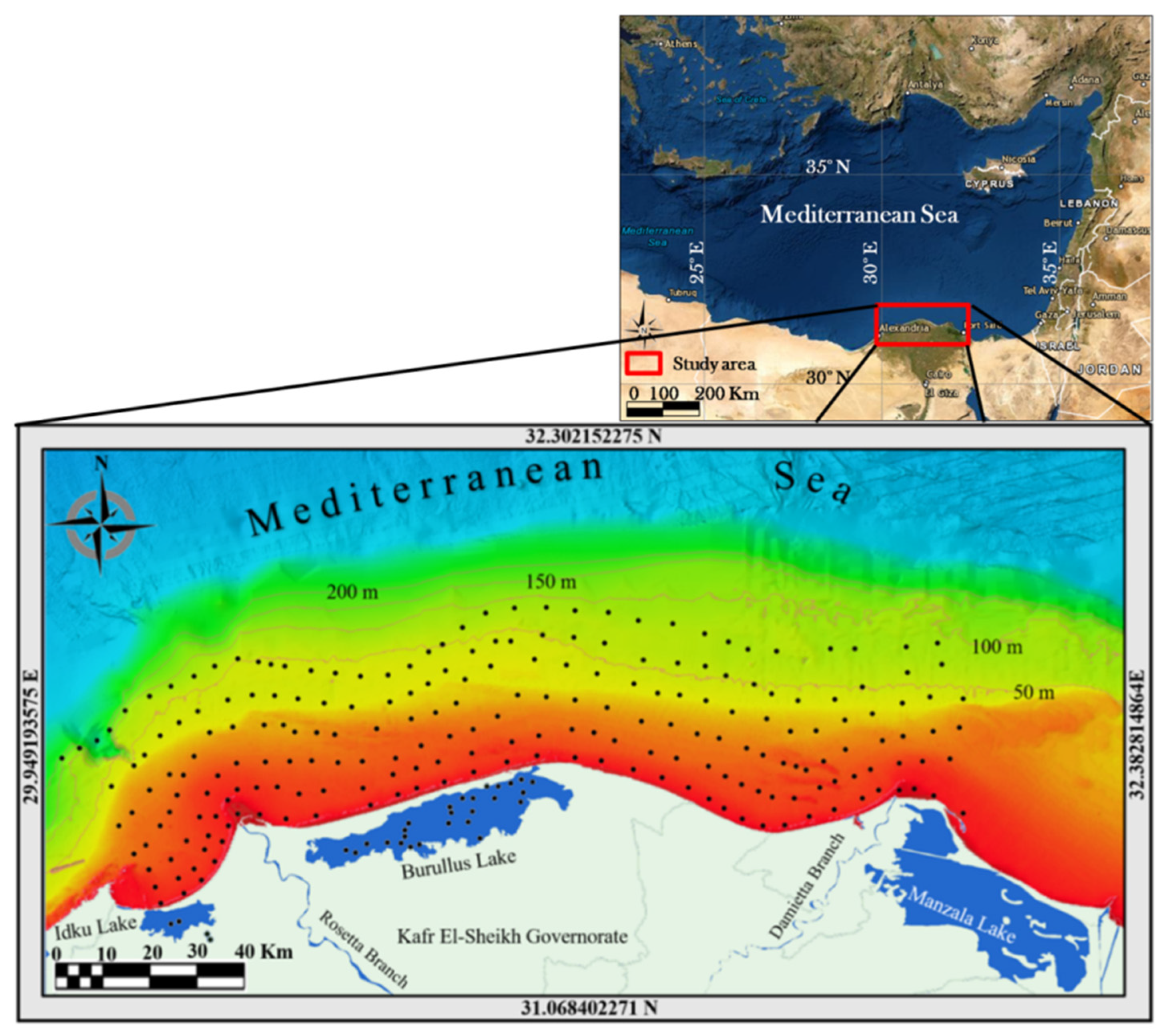
2.1. Study Area

The region of interest is located on the Mediterranean coast of the Nile Delta and its fringes with a special focus on the Burullus Lake environment representing the inland lake waters (Figure 1). Higher values of biomass, and consequently of Chl-a, may be found in areas influenced by watercourses runoff into the study area, which was selected because of its complex water dynamics and its dense anthropogenic pressure. Burullus Lake is the second largest of the northern coastal lakes along the Mediterranean coast of Egypt, covering about 420 km² commonly used for fishing and recreation activities. The lake is covered by floating vegetation, isolated sand bars, urban areas, and agriculture lands.

The physical and biological characteristics of the lake has been recently documented by Masoud et al. [65]. The lake water showed a depth average of 130.5 cm with a range level of 0.90–2 m, alkaline pH (7.78–8.92), and average salinity of 4.33 gm/L with a range of 0.3–17.19 gm/l. The phytoplankton displayed a high level of variation in the number of taxa (145 species) and abundance with maximum counts of 1005 × 10³ units.L⁻¹ to a minimum of 340 × 10³ units.L⁻¹. Six groups of freshwater forms dominated by the Chlorophyceae, Bacillariophyceae, Cyanophyceae, Dinophyceae, Euglenophyceae, and Silicoflagillate, were arranged in decreasing order of abundance.

2.2. Satellite Data and Image Processing

Different data sets of S3A/OLCI, S2A/MSI, and L8/OLI imagery were searched and allocated for atmospheric correction assessment (Figure 2). The imagery file naming, processing levels and sensing time are shown on

Table 1. Remote Sensing data acquired over North of the Nile Delta of Egypt.

	Sensor	Product Name	Level	Sensing Date/Time
Coastal Water	S3 OLCI Earth Observation Full Resolution Product (EFR)	S3B_OL_1_EFR_20200322T075148_20200322T075448_20200323T120250_0180_037_035_2340_LN1_O_NT_002.SEN3	Level-1	22 March 2020 07:51:48.398789
	S3 OLCI Water Full (OL_2_WRF) Resolution products (WFR)	S3B_OL_2_WFR_20200322T075148_20200322T075448_20200323T134658_0180_037_035_2340_MAR_O_NT_002.SEN3	Level-2	22 March 2020 07:51:48.398789
	Landsat-8 OLI	LC08_L1TP_177038_20200322_20200326_01_T1	Geometrically corrected	22 March 2020 08:29:26
	S2 MSI 1C	S2A_MSIL1C_20200322T083621_N0209_R064_T36RTV_20200322T104149.SAFE S2A_MSIL1C_20200322T083621_N0209_R064_T36RUV_20200322T104149.SAFE S2A_MSIL1C_20200322T083621_N0209_R064_T36SUA_20200322T104149.SAFE S2A_MSIL1C_20200322T083621_N0209_R064_T36STA_20200322T104149.SAFE	Level 1C	22 March 2020 08:36:21.024Z
	MODIS	A2020082111000.L2_LAC_OC.nc	Level 3	11:10:00.976Z
Inland Water	S2 MSI 1C	S2A_MSIL1C_20200918T083621_N0209_R064_T36RTV_20200918T101859.SAFE	Level 1C	18 September 2020
	S2 MSI 1C	S2B_MSIL1C_20200920T082629_N0209_R021_T36RUV_20200920T104059.SAFE	Level 1C	20 September 2020

. The sensing time period was 45 min for the three data sets, starting from 7:51 to 8:36 AM acquired on 22 March 2020. Image processing was carried out for the Landsat-8 Operational Land Imager (OLI) and for two Sentinel sensors developed by the European Space Agency (ESA) as part of the Copernicus Earth Observation Programme for the monitoring of natural water bio-optical properties: Sentinel-2 Multi-Spectral Instrument (S2-MSI) and Sentinel-3 Ocean and Land Color Instrument (S3-OLCI) [66,67]. The sensors slightly vary in the bandwidths and their spectral locations, as indicated in

Table 2. Visible NIR spectral band characteristics of the studied data as depicted on their user hand books.

OLI	S2 MSI			S3 OLCI
30 m	10 m	20 m	60 m	300 m	λ Range (nm)	Function
λ (nm)	λ (nm)	λ (nm)	λ (nm)	λ (nm)
				400	392.5–407.5	Aerosol correction, improved parameter retrieval
				412.5	407.5–417.5	Yellow substance and detrital pigments (turbidity)
440		B1	443	442.5	437.5–447.5	Chlorophyll-a absorption max.
490	490	B2		490	485–495	High Chl and other pigments
				510	505–515	Chl, sediment, and turbidity
560	560	B3		560	555–565	Chl reference (Chl minimum)
				620	615–625	Sediment loading
665	665	B4		665	660–670	Chl (2nd Chl abs. max.), sediment, yellow substance
				673.5	670–677.5	For improved fluorescence retrieval
				681.25	677.5–682	Chl fluorescence peak, red edge
	B5	705		708.75	703.75–713.75	Chl fluorescence baseline, red-edge transition
	B6	740		753.75	750–757.5	O2 absorption/clouds, vegetation
				761.75	760–762.5	O2 absorption band/aerosol correction
				764.75	762.5–766.25	Atmospheric correction
				767.75	766.25–768.75	O2 used for cloud top pressure, fluorescence over land
		783	B7	778.75	771.25–786.25	Atmos. corr./aerosol correction
865	842	865	B8 B8A	865	855–876	Atmos. corr./aerosol corr., clouds, pixel co-registration
B5				885	880–890	Water vapor absorption reference band.
				900	895–905	Water vapor absorption (max. reflectance)
		B9	940	940	930–950	Water vapor absorption, atmos./aerosol correction.
				1020	1000–1040	Atmos./aerosol correction.

.

The Landsat-8 signal-to-noise ratio (SNR) has been shown to increase significantly with narrower bandwidth compared to Landsat’s previous missions in the red and near-infrared (NIR), among others, and attains radiation resolution, increasing to 16 bits with a 16-day repeat cycle. All advances have attributed to improved pigment discrimination ability, which have proven useful for estimating concentrations of Chl-a in water bodies [53,68].

The Sentinel-2 Multi-Spectral Instrument (S2MSI) attains a high 12-bit radiometric resolution, wide spatial and temporal resolution; the location and bandwidth are narrower compared to the OLI data and has a wide field of view (FoV) that generates spectral images composed of 13 bands at high SNR and varying wavelengths (Table 2). The use of S2-MSI images has been common in monitoring lakes and rivers and in developing predictive models for Chl-a (e.g., [69,70,71,72,73,74]). Cloud-free imageries were only available from the S2MSI acquisitioned within the same week of in situ sampling from 55 stations, on 18 September 2020 for the western part, and on 20 September for the eastern part of the inland Burullus Lake, that was validated against ground-truth in situ data.

The Sentinel 3 OLCI has two sets of data: unprocessed earth full resolution (EFR) data and the processed for water full resolution products (WFR). The OLCI large number of bands improve the atmospheric correction over the optically-complex waters [75], O₂ gas absorption correction, and the water constituents’ retrieval. The ready-to-use OLCI Chl-a data have two products derived by applying the Neural Network (NN) Inverse Radiative Transfer Model (e.g., [76,77,78]) and the Ocean Color 4 for MERIS (OC4Me) of the chlorophyll-a (Chl-a), a semi-analytical model that is based on a polynomial algorithm that uses a maximum band ratio approach of reflectances at 443, 490, and 510 nm over the 560 nm [79] based on the analysis of AOPs measured in situ over the past decades in various oceanic regions (e.g., [79,80]).

The surface Chl-a of the Copernicus Marine Environment Monitoring Service (CMEMS), S3 WFR, and the MODIS are used as reference standard for evaluation. The Chl-a concentration of the coastal water estimated on 22 March 2020 sampled daily at a spatial resolution of 0.042 degrees is analyzed from the CMEMS data available at (https://resources.marine.copernicus.eu/product-detail/MEDSEA_ANALYSISFORECAST_BGC_006_014, last accessed 1 January 2022). The remotely-sensed water geochemical parameters of the pH, alkalinity, dissolved inorganic carbon, zooplankton biomass, chlorophyll-a, phytoplankton biomass, nitrate, phosphate, silicate, and ammonia is used for correlation and regression analysis. The MODIS Aqua measurements Level 3 (4 km), downloaded from the ocean color website (https://oceancolor.gsfc.nasa.gov/) were acquired on 22 March 2020 from 11:10 to 11:14 a.m.

A flowchart explaining the adopted methods and associated steps is shown on Figure 3.

All sensor data were first masked for clouds and cloud shadows, and subsequently atmospherically corrected using the C2RCC atmospheric correction scheme. The algorithm runs on the visible-NIR bands (Table 2) commonly used for water color retrieval, with 5 bands for the OLI data, the MSI has 9 bands out of the sensor 13 bands at 10-60 m grid spacing, while OLCI has the 21 spectral bands in this region at a resolution of 300 m [81]. The satellite imageries were geometrically corrected to the UTM Zone 36, resampled, to 10 m resolution for MSI, 30 m for OLI, and 300 m for OLCI EFR; all were then subset to the study area. The land and cloud covers were masked using the metadata associated with the imageries. The atmospheric correction was then applied by appraising the use of the C2RCC algorithm implemented in the Sentinel Application Platform (SNAP) version 5.0 with the Sentinel-3 Toolbox Kit Module (S3TBX) version 5.0.1 for the three sensor data sets. Simply, C2RCC is based on water radiative transfer modeling and the vector successive order of scattering (SOS) atmospheric model with aerosol optical properties derived from NASA AERONET-OC measurements [82,83]. The artificial neural network technology [84,85] is used where for every sensor data, a subset of bands is set as neural nets; the main net derives water-leaving reflectance ‘ρ_w(λ)’ and the top-of-atmosphere (TOA) ρ_toa(λ) radiances after atmospheric correction with an elaborate bio-optical ocean–atmosphere model using a large database of water-leaving reflectances and relating to the optical properties from various coastal areas around the world. Subsequently, the trained neural nets parametrize the inverse relationship between inherent optical properties (IOPs) and reflectances (water-leaving ρ_w(λ) from the ρ_toa(λ)), allowing the retrieval of certain water quality parameters, such as chlorophyll-a, TSM, and the CDOM [86].

For all combination of the IOP components, based on a large world database of radiative transfer simulations in natural waters as “truth”, and the trained IOP inversion net as “estimate”, the difference between truth and estimate gives the uncertainty per IOP per pixel in the image [82], defined here as the associated error of the water color constituent. C2RCC proved applicable to a wide range of satellite sensors, such as SeaWiFS, MERIS, MODIS, OLI, MSI, and OLCI [85], and efficient in many world case studies for the retrieval of Ocean Color estimates; detailed information on processing is given in Brockmann et al. [85].

For the C2RCC implemented in SNAP, the local relationship between IOPs and concentrations of optical substances in the water that are regionally variable can be adjusted by adapting the ancillary parameters to local waterbody specific inherent optical properties (sIOPs), such as salinity, temperature, ozone, air pressure as well as the specific IOPs, namely the Chl-specific absorption coefficient and the specific scatter of TSM at 442 nm. For this study, the coastal water salinity was set to 39 PSU and the water temperature was set to 21.5 °C as common values for the study area in the Mediterranean Sea stated in several studies, which is different from the default setting (e.g., [87]) and the sea surface data of the European Organization for the Exploitation of Meteorological Satellites (EUMETSAT) for temperature; [88] for salinity). EUMETSAT data is available at https://www.eumetsat.int/S3b-sst-processing-baseline, last accessed 1 January 2022. The values of temperature and salinity of the studied period and the examined area investigated using the Copernicus products sampled hourly at a spatial resolution of 0.042 degrees (https://resources.marine.copernicus.eu/?option=com_csw&view=details&product_id=MEDSEA_ANALYSISFORECAST_PHY_006_013, last accessed 1 January 2022) were comparable to the values set for the analysis. The average values of temperature and salinity of Burullus Lake were set from in situ measurements [65], sampled in the period 22–25 March 2020 as 28.8 °C and 4.32 PSU, respectively.

After the AC and prior to pixel extraction, MSI and OLI pixels were resampled to 300 m and registered to match the OLCI georeferenced image to allow inter-comparison.

2.3. Inter-Sensor Comparison and Validation in Burullus Lake

Due to a lack of ground-truth data for the March 2020 sensor data, metrics of the Pearson correlation coefficients (r), least-square coefficient of determination (R²) of multivariate regression analyses, along with the mean absolute error (MAE), and the root mean square error (RMSE) were employed and evaluated for sampling location points among the three sensor-based empirical models and compared with the standard measurements of the CMEMS, OLCI WFR, and MODIS data in order to examine the accuracy and cross-method consistency of water quality products.

The MAE and the RMSE metrics indicate the relative error of estimates and account for the proportionality of the errors with the concentration of the constituents.

Equations (1) and (2) are used for estimating the MAE and RMSE, respectively.

$$\mathrm{MAE}=\frac{1}{N}{\displaystyle \sum }_{i=1}^N|x_i-y_i|$$

(1)

$$\mathrm{RMSE}=\sqrt{\frac{1}{N}{\displaystyle \sum }_{i=1}^N{\left(x_i-y_i\right)}^2}$$

(2)

where N is the number of sample points, y_i is the estimated water color parameter from the three data sets, and x_i is the value of water color value of the standard products.

Sampling of 275 locations in the coastal water and 30 points in the inland Burullus Lake were extracted from the overlapping region of the data footprints through on-screen digitizing selected to cover varying optical contents, water depths, and varying distances from the downstream areas of the inland watercourses. For validation in the inland lake water, in situ data from 55 sampling points across Burullus Lake, collected during 22–25 September 2020, were used [65] for evaluating the water products retrieved from the S2 MSI image acquired on 18–20 September 2020, where r, R², RMSE have been quantified.

3. Results

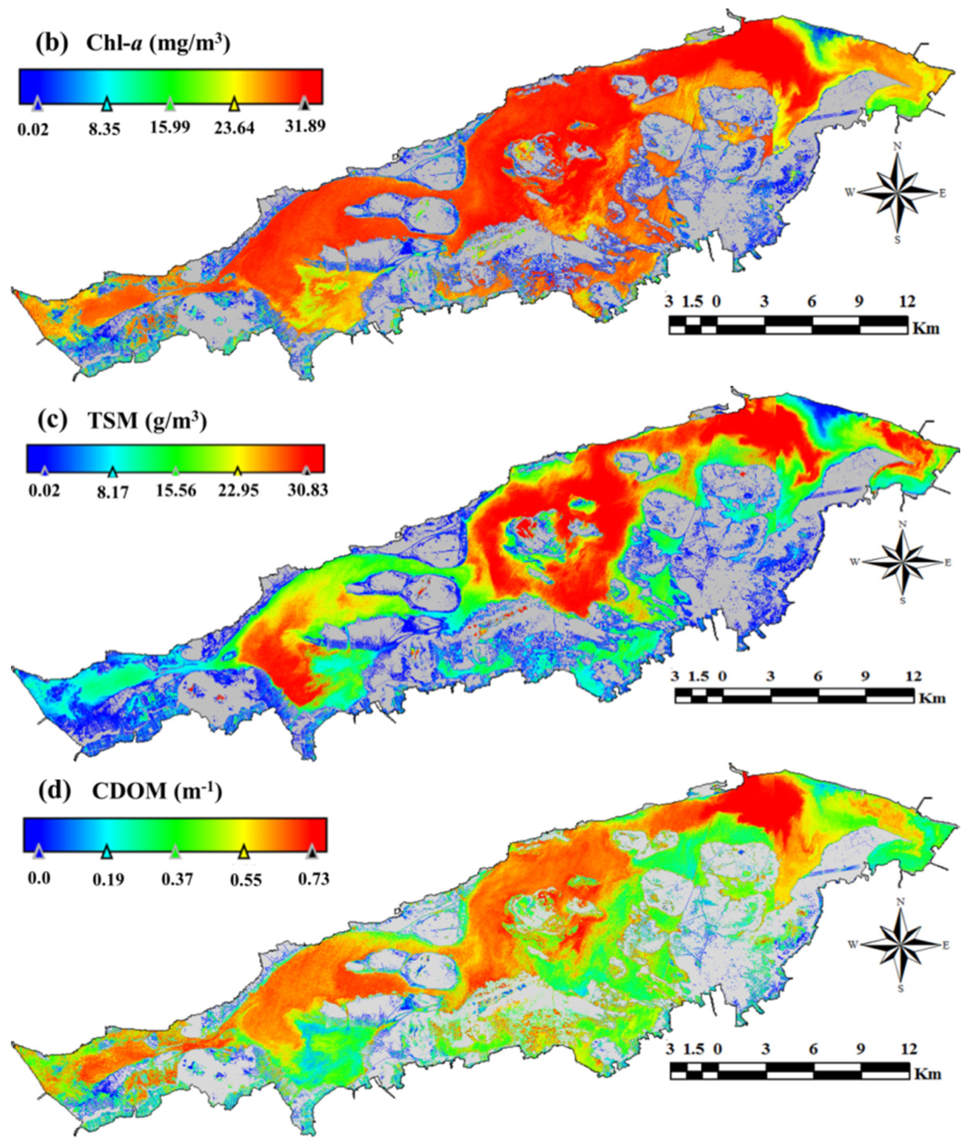
3.1. Distribution of Retrieved Water Color Parameters

Retrieved water color parameters of Chl-a, TSM, and CDOM along with their associated errors are shown for the S2MSI (Figure 4), selected for display to attain the finest resolution of 10 m among all data. The distribution of the retrieved parameters for the S3 OCLI (WFR and EFR), OLI, and MODIS are shown in the Supplementary file to this article. The distribution of water content was uneven with the maximum concentrations marked by the inland lake water and the downstream areas located in front of the outlet of the northern lakes into the coastal water, close to the shoreline.

The Chl-a content showed a gradual decrease with a depth pattern parallel to the coastline, where local highs are located in front of the Rosetta and Damietta promontories and Boughaz El-Burullus (Figure 4). The patterns of concentrations in all investigated sensors and reference data were congruent and showed similar trends in the coastal water and varied widely in the inland lake and fish farm waters.

Assessing the retrieved parameters for the 275 sampling points in the coastal water clarified that the Chl-a content averaged 3.14 mg m⁻³ in the range level of 0.39–4.81 mg m⁻³ for all data. TSM clarified a mean of 7.66 g m⁻³ ranging from 6.32 g m⁻³ to 10.18 g m⁻³. CDOM averaged 0.18 m⁻¹ with a range level of 0.13–0.30 m⁻¹ (

Table 3. Summary Statistics of the Chl-a, TSM, and CDOM contents estimated from the EFR, MSI, and OLI along with the reference standard CMEMS, WFR, and MODIS for the 275 sampling points in the coastal water.

		CMEMS	WFR (NN)	WFR (OC4Me)	MODIS	EFR	MSI	OLI
Chl-a (mg m−3)	Min	0.08	0.08	0.13	0.15	0.06	0	0.04
	Max	2.13	18.86	30.22	18.51	21.52	17.64	14.46
	Mean	0.39	3.92	4.81	3.37	2.69	4.06	2.76
	Std. error	0.03	0.25	0.38	0.27	0.19	0.39	0.25
	Variance	0.13	16.78	38.1	16.26	9.49	20.55	13.41
	Stand. dev	0.36	4.1	6.17	4.03	3.08	4.53	3.66
	25 prcntil	0.12	0.19	0.32	0.3	0.21	0.18	0.18
	75 prcntil	0.52	7.35	6.83	4.37	4.19	7.86	3.39
	Skewness	2.1	0.69	1.92	1.57	2.79	0.79	1.66
	Kurtosis	5.45	−0.59	3.87	1.87	12.52	−0.5	1.88
TSM (g m−3)	Min		0.32		0.16	0.05	0.12	0.16
	Max		45.03		51.21	63.63	28.85	51.21
	Mean		10.18		6.32	7.77	7.7	6.32
	Std. error		0.67		0.47	0.72	0.55	0.47
	Variance		115.43		59.84	73.64	64.47	59.84
	Stand. dev		10.74		7.74	8.58	8.03	7.74
	25 prcntil		1		0.64	0.78	0.54	0.64
	75 prcntil		19.56		9.28	12.71	14.43	9.28
	Skewness		0.76		2.38	2.3	0.63	2.38
	Kurtosis		−0.67		8.38	11.3	−1.06	8.38
CDOM (m−1)	Min		0.02		0.01	0	0.01	0.01
	Max		2.12		0.75	0.78	0.66	0.75
	Mean		0.30		0.13	0.21	0.13	0.13
	Std. error		0.02		0.01	0.02	0.01	0.01
	Variance		0.12		0.01	0.04	0.02	0.01
	Stand. dev		0.34		0.12	0.2	0.13	0.12
	25 prcntil		0.04		0.01	0.02	0.01	0.01
	75 prcntil		0.5		0.2	0.38	0.23	0.2
	Skewness		1.91		1.54	0.6	1.24	1.54
	Kurtosis		5.53		4.65	−0.9	1.42	4.65

NB: Values are highlighted from largest (red) to smallest (blue). Significance level of p = 95% is adopted.

).

With focus on the large scale of 10 m S2MSI data (Figure 4), as was clear on all sensor data, bloom areas of Chl-a, TSM, and CDOM characterize the Rosetta promontory and Boughaz El-Burullus which discharge large amounts of water of intense nutrient loads into the sea, in particular, nitrogen and phosphorous compounds of vital importance to phytoplankton growth and productivity. A recent study by [65] indicated that Burullus Lake is demarcated with wide Chl-a blooms (av. 83.4 mg.m⁻³ and range levels of 53.76–129 mg.m⁻³) intensified by the inflow from agricultural drains in the east, and a fresh Nile water canal in the west. Chl-a concentrations of 2.144 mg m⁻³ indicated a phytoplankton bloom in the Southern Ocean [89].

Based on this value, marked blooms can be easily mapped and their controlling factors can be spatially better understood. These blooms, as indicated in our recent study, can be used in efficient monitoring of the harmful algal blooms and their biological contents of carbohydrates, lipids, and protein can be utilized for the phytoplankton bioenergy potential mapping practices.

3.2. Inter-Sensor Data Comparison

Inter-comparison of retrieved parameters applying C2RCC over optically different water types proved successful in the open coastal water, while revealing problems for the inland lake water with estimating accurate variables induced mostly by the adjacency effect and the optical dominance of the CDOM absorption, which cause lower reflectances.

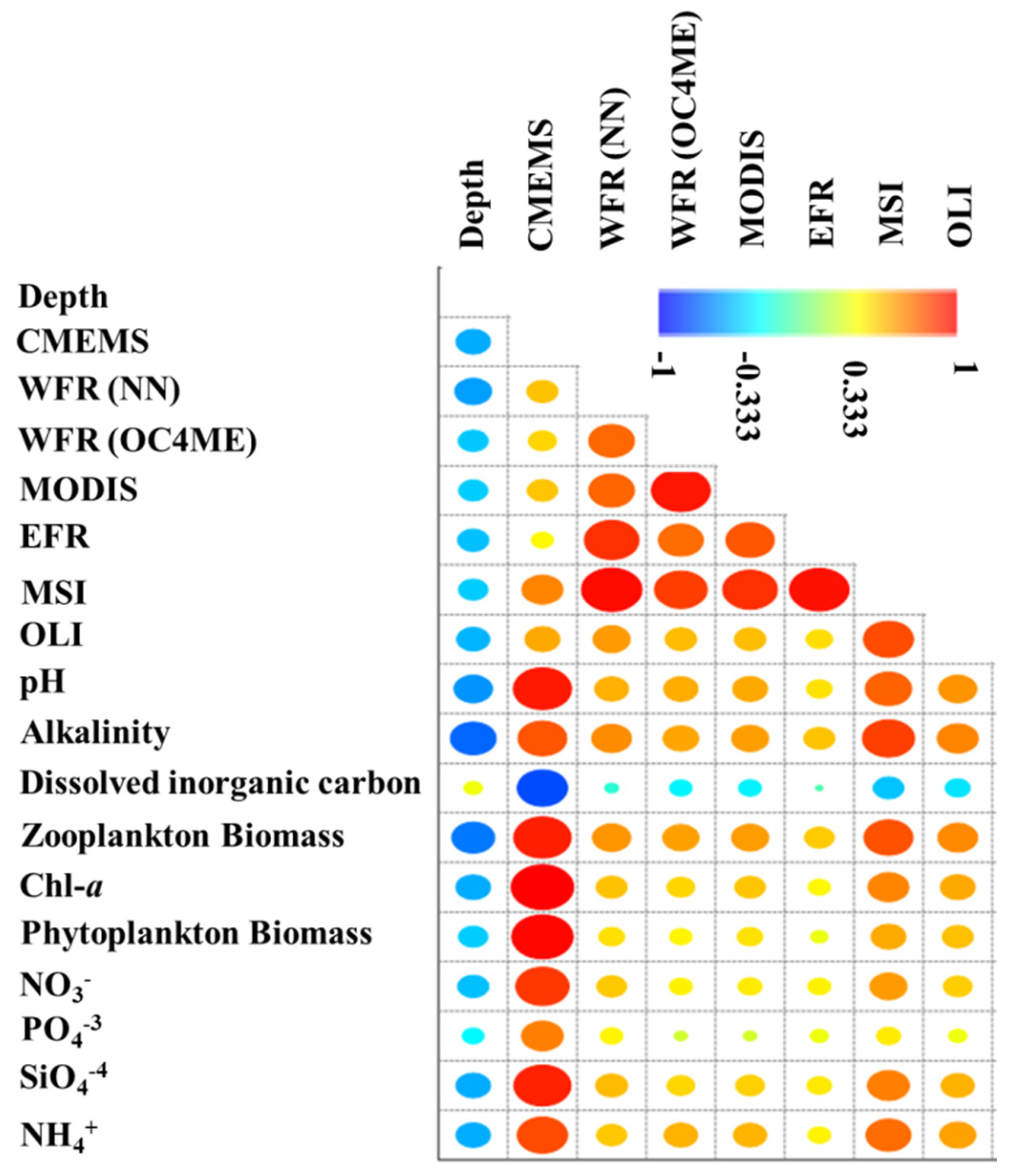
3.2.1. Correlation Analysis

Correlation analysis for 275 sampling points visually selected to cover varying depths along the coastal waters clarified that the Chl-a contents attained the most inferior coefficients for the reference CMEMS and the estimated OLI contents among all data (

Table 4. Pearson’s correlation coefficients of the coastal water quality parameters estimated from EFR, MSI, and OLI against the reference standard CMEMS, WFR, and MODIS parameters (n = 275).

		CMEMS	WFR (NN)	WFR (OC4Me)	MODIS	EFR	MSI	OLI
Chlorophyll-a	CMEMS
	WFR (NN)	0.49
	WFR (OC4Me)	0.44	0.73
	MODIS	0.49	0.73	0.94
	EFR	0.35	0.87	0.72	0.77
	MSI	0.65	0.97	0.84	0.88	0.95
	OLI	0.56	0.6	0.51	0.5	0.42	0.80
TSM	WFR (NN)
	EFR		0.94
	MSI		0.84			0.92
	OLI		0.93			0.69	0.87
CDOM	WFR (NN)
	EFR		0.79
	MSI		0.93			0.80
	OLI		0.60			0.51	0.80

NB: Values are highlighted from largest (red) to smallest (blue). Significance level of p = 95% is adopted.

). MSI ranked first with strongest significant coefficients of Chl-a contents among all data (r = 0.65–0.97) with stronger correlation against WFR (NN) (r = 0.97) followed by EFR (r = 0.95), MODIS (r = 0.88), WFR (OC4Me) (r = 0.84), OLI (r = 0.80), and CMEMS (r = 0.65). In terms of the TSM, EFR clarified the strongest positive coefficients against the WFR (NN) (r = 0.94), MSI (r = 0.92), and OLI (r = 0.69), arranged in decreasing order.

MSI proved second in rank where it showed strong positive correlation against WFR (r = 0.84) and OLI (r = 0.87). MSI proved superior over all sensors for estimating the CDOM content against WFR (NN) (r = 0.93), EFR (r = 0.80), and OLI (r = 0.80). Correlating the Chl-a contents among estimated and reference data (

Table 5. Pearson’s correlation coefficients among estimated and reference Chl-a contents and coastal water geochemistry (CMEMS).

	Depth	CMEMS	WFR (NN)	WFR (OC4ME)	MODIS	EFR	MSI	OLI
Depth
CMEMS	−0.55
WFR (NN)	−0.81	0.49
WFR (OC4ME)	−0.66	0.44	0.68
MODIS	−0.68	0.49	0.69	0.93
EFR	−0.68	0.35	0.85	0.67	0.74
MSI	−0.80	0.65	0.97	0.83	0.87	0.95
OLI	−0.55	0.56	0.56	0.47	0.46	0.37	0.79
pH	−0.61	0.93	0.54	0.55	0.56	0.41	0.74	0.61
Alkalinity mol m−3	−0.73	0.78	0.63	0.57	0.59	0.49	0.84	0.66
Dissolved inorganic carbon mol m−3	0.30	−0.81	−0.22	−0.36	−0.37	−0.12	−0.49	−0.4
Zooplankton Biomass	−0.69	0.92	0.61	0.58	0.59	0.47	0.78	0.64
Chl-a mg m−3	−0.55	1	0.49	0.44	0.49	0.35	0.65	0.56
Phytoplankton Biomass mmol m−3	−0.47	0.98	0.41	0.36	0.41	0.28	0.56	0.50
NO3− mmol m−3	−0.50	0.85	0.48	0.37	0.39	0.37	0.59	0.46
PO4−3mmol m−3	−0.35	0.67	0.36	0.21	0.22	0.29	0.39	0.30
SiO4−4mmol m−3	−0.55	0.91	0.51	0.44	0.46	0.39	0.67	0.53
NH4+mmol m−3	−0.55	0.81	0.48	0.54	0.53	0.37	0.72	0.58

NB: Values are highlighted from largest (red) to smallest (blue). Significance level of p = 95% is adopted.

and Figure 5) against the coastal water geochemistry (CMEMS) clarified a decreasing trend with depth, with strongest correlation marked by the WFR (NN) and MSI data (r => 0.80). MSI estimates are by far the strongest significant positive coefficients against all parameters, following in rank that against the reference CMEMS Chl-a contents (Table 5).

3.2.2. Regression Analysis

The satellite sensors also clarified overall good performance in the retrieval of Chl-a, TSM, and CDOM in the visible and NIR bands, which proved optimal in deriving the water color parameters. Regression analysis of the Chl-a contents of the EFR, MSI, and OLI against the reference standard CMEMS, WFR, and MODIS clarified that the MSI estimates are advantageous over all data followed by EFR, where OLI came last in rank (Figure 6). MSI showed best fits against WFR (NN) (R² = 0.94), MODIS (R² = 0.77), WFR (OC4Me) (R² = 0.71), and CMEMS (R² = 0.43), in decreasing order.

Regression analysis of the TSM and CDOM (

Table 6. Coefficients of determination (R²) of the retrieved TSM and CDOM parameters in the coastal water (n = 275).

	EFR		OLI		MSI
	TSM	CDOM	TSM	CDOM	TSM	CDOM
WFR	0.90	0.63	0.66	0.63	0.86	0.73
EFR			0.70	0.30	0.82	0.42
OLI					0.91	0.70

) clarified that the TSM estimates of MSI proved advantageous over all sensors with best fits (R²) in the range level of 0.82–0.91, being maximum against OLI (R² = 0.91), followed by WFR (R² = 0.86), and EFR (R² = 0.82). CDOM estimates best fitted with WFR (R² = 0.73), OLI (R² = 0.70), and EFR (R² = 0.42), in a decreasing order. The R² proved low for the retrieved parameters in Lake Burullus compared to that in the coastal marine water (

Table 7. Coefficients of determination (R²) of the retrieved parameters in Lake Burullus (n = 30).

.	EFR			MSI			OLI
	Chl-a	TSM	CDOM	Chl-a	TSM	CDOM	Chl-a	TSM	CDOM
WFR	0.59	0.10	0.09	0.32	0.27	0.36	0.18	0.14	0.01
EFR				0.45	0.011	0.003	0.00	0.00	0.02
OLI				0.07	0.632	0.22

Values of Chl-a are shown in green, TSM in red, and CDOM in orange.

).

3.2.3. Retrieval Performance Analysis Metrics

Over all the investigated sensors with local water salinity and temperature inputs in the coastal water, MSI ranked first achieving the smallest MAE and RMSE for the Chl-a contents, while the EFR proved superior with lowest MAE and RMSE for TSM and CDOM estimates (

Table 8. Water quality estimation performance analysis metrics (MAE and RMSE) in the coastal water.

		CMEMS	WFR (NN)	WFR(OC4Me)	MODIS	EFR	MSI	OLI	CMEMS	WFR (NN)	WFR(OC4Me)	MODIS	EFR	MSI	OLI
		MAE							RMSE
Chlorophyll-a	CMEMS
	WFR (NN)	3.38							5.13
	WFR (OC4Me)	4.2	0.93						7.31	4.27
	MODIS	2.37	0.47	1.04					4.38	2.67	2.35
	EFR	2.14	1.15	2	0.62				3.61	2.3	4.73	2.41
	MSI	1.73	0.49	0.50	0.12	0.90			3.81	1.3	2.7	1.32	2.3
	OLI	1.65	1.19	2.18	0.77	0.15	0.67		3.48	3.45	5.61	3.34	3.29	2.12
TSM	WFR (NN)					1.17	1.54	1.78					2.54	5.27	4.29
CDOM	WFR (NN)					0.20	0.21	0.22					0.37	0.43	0.44

NB: Values are highlighted from largest (red) to smallest (blue).

).

3.3. Burullus Lake Water Quality Parametrs

Spatial distribution of the water quality parameters for the Chl-a, TSM, and CDOM content in Burullus Lake is shown on Figure 7.

The in-situ data indicated that the Burullus Lake water is hypertrophic with a wide variation of Chl-a blooms (av. 83.4 mg.m⁻³ and range levels of 53.76–129 mg.m⁻³). The MSI-estimated that Chl-a showed a range level of 0.08–38.52 mg.m⁻³ with average of 27.83 mg.m⁻³ (

Table 9. Summary statistics of the MSI Chl-a, TSM, and CDOM contents and the in-situ measured chlorophyll-a in Burullus Lake.

	S2 MSI			In-Situ
	Chl-a	TSM	CDOM	Chlorophyll a (mg.m−3)
Min	0.08	0.33	0.11	53.76
Max	38.52	35.31	0.78	129.03
Mean	27.83	20.47	0.52	83.43
Std. error	1.03	1.46	0.02	2.57
Stand. dev	7.55	10.73	0.16	19.09
25 prcntil	26.59	11.21	0.38	66.05
75 prcntil	32.04	29.79	0.64	97.03
Skewness	−2.09	−0.46	−0.72	0.39
Kurtosis	4.65	−1.15	−0.35	−0.61

). This confirmed a clear underestimation in the level range of 0.1–59% and average of 35.35% of the Chl-a, which becomes large at larger in situ Chl-a concentrations. Correlation analysis shown on

Table 10. Pearson’s correlation coefficients of in situ measured and S2 MSI-derived water quality parameters in Burullus Lake.

	Chl-a (mg.m−3)	TSM (g/m3)	CDOM (m−1)
MSI Chl-a (mg.m−3)
TSM	0.71
CDOM	0.68	0.37
TDS	0.07	0.17	−0.25
T°C	−0.17	−0.24	−0.38
Bacillariophyceae	−0.2	−0.37	−0.08
Chlorophyceae	−0.11	−0.22	−0.19
Euglenophyceae	−0.35	−0.56	−0.22
Total algae	−0.25	−0.46	−0.23
Measured Chlorophyll a (mg.m−3)	−0.16	−0.36	−0.21
Proteins (mg/L)	−0.24	−0.49	−0.21
Carbohydrates (mg/L)	−0.22	−0.36	−0.33
Lipids (mg/L)	−0.16	−0.25	−0.24

NB: Values are highlighted from largest (red) to smallest (blue). Significance level of p = 95% is adopted.

indicated that the MSI-derived Chl-a contents are much affected by the TSM (r = 0.71) and CDOM (r = 0.68) contents. Fair to weak, either positive or negative coefficients are clarified between the estimated water quality parameters against the in situ measured lake water variables (e.g., TDS, T°C, algal composition and abundance, and biological contents of Chl-a, proteins, carbohydrates, and lipids).

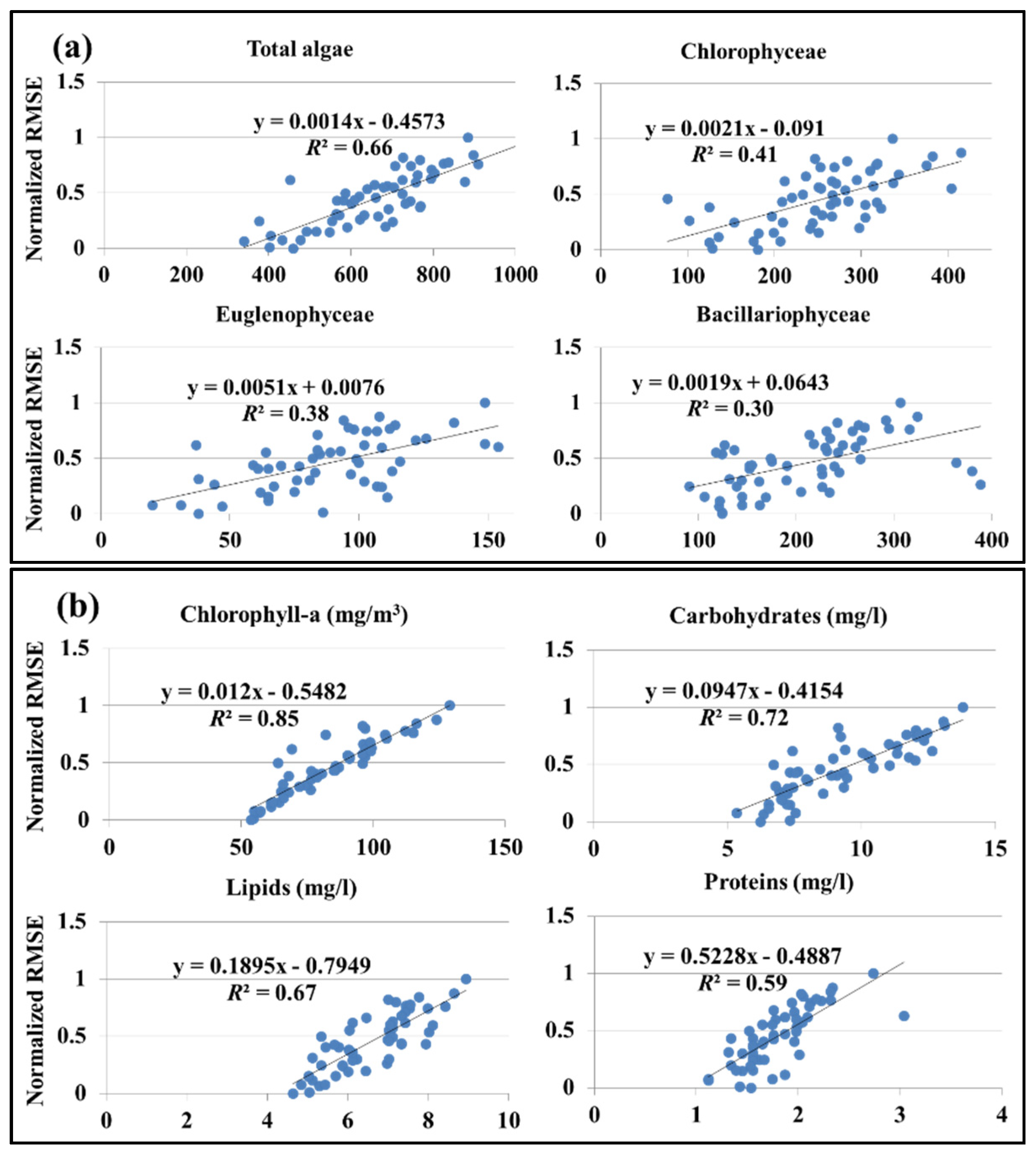
3.4. Validation and RMSE Characterization

The RMSE between measured and estimated Chl-a content was then estimated, normalized between minimum and maximum values, and regressed against some lake water variables to characterize possible factors enhancing the disagreement magnitudes at the 55 sampling stations taking the spatial distribution of the in situ measured Chl-a contents as reference. The normalized RMSE was then mapped and lake water factors inducing retrieval of water quality parameters were identified and characterized.

Regression analysis of the normalized RMSE against algal composition and abundance (counts) and algae biological contents in Burullus Lake (Figure 8) clarified the determination coefficient with best fit against total algal counts (R² = 0.66), followed by the Chlorophyacea (R² = 0.41), Euglenophycaea (R² = 0.38), and Bacillariophycaea (R² = 0.30). The NRMSE showed best fit against the in situ measured Chl-a content (R² = 0.85), carbohydrates (R² = 0.72), lipids (R² = 0.67), and proteins (R² = 0.59), in decreasing order. The underestimation increased at larger estimates of algal composition and abundance, and biological contents.

The largest Chl-a contents associated with largest normalized RMSE estimates marked the downstream areas where the inflow of polluted water persistently brings nutrients loads of nitrogen and phosphorous compounds as well as substantial amounts of detrital particles and sediments flowing from the agricultural and industrial drains into the lake shallow zones from the south and east causing re-suspension of bottom sediments in the water column, resulting in the increase of water turbidity, and giving rise to inaccurate Chl-a estimates (Figure 9). These areas attained the largest contents of algal composition and abundance of total algal counts dominated by Chlorophyacea, Euglenophycaea, and Bacillariophycaea, which clarify largest biological contents of carbohydrates, lipids, and proteins. The intense environmental pollution marked by intense eutrophication dominates large error-prone areas mostly linked to climatic, hydrologic fluctuation of the drain water flows most affected by wind direction and turbulent water intermixing regimes, and associated nutrient load discharged from land use changes to fish farms and the related agricultural practices south of the lake. The dynamicity in shallow (<2 m depth) water spatio-temporal turbidity and associated pollution loads hindered accurate estimates of the lake water quality parameters from the S2 MSI imagery applying the C2RCC algorithm.

4. Discussion

The used multi-sensor data proved promising to a large extent of success for the retrieval assessment of the complex case 2 coastal water quality parameters, including Chl-a, TSM, and CDOM. Mean of 3.14 mg m⁻³, 7.66 g m⁻³, and 0.18 m⁻¹ with range levels of 0.39- 4.81 mg m⁻³, 6.32–10.18 g m⁻³, and 0.13–0.30 m⁻¹ were estimated for the Chl-a, TSM, and CDOM, respectively. In situ Chl-a data available from recent local reports and literature clarified good agreement with the mean and the range level estimated in the present research. The Egyptian Environmental Affairs Agency (EEAA) report in 2019 for the Mediterranean coast of Egypt (https://www.eeaa.gov.eg/en-us/mediacenter/reports/projectstudies/eimp.aspx, last accessed on 28 January 2022) clarified a yearly Chl-a average of about 2 mg m⁻³ and range level of 0.42–5.33 mg m⁻³. In addition, in situ monthly Chl-a from March 2019 to February 2020 at the beaches in Alexandria [90], located on the western part of the study area’s coastal water clarified an average of 2.47 with a range level of 1.37–3.19 mg m⁻³. Further, in situ Chl-a measurements for 692 points distributed in the Mediterranean Sea showed a range level of 0.01–4 mg m⁻³, which were comparable to Chl-a estimated from the S3 OLCI and the CMEMS data acquired between the years 2016–2018 [91].

Sensor differences in spatial and spectral samplings, induced and disclosed how well the sensors are suited for the seamless generation of the water quality parameters. The C2RCC provided the pixel-wise certainty level of the estimated parameter concentration and also the associated uncertainty. The certainty maps provide a support to understand the challenges in ocean color monitoring by the studied sensors where these certainty maps can be used as a mask, to disregard areas with relative high uncertainties, and keep the estimates, where the computed statistical measures are valid. C2RCC was originally developed for marine waters using bands at the blue and green regions of the electromagnetic spectrum [92].

In the coastal water, close and parallel to the shoreline, C2RCC proved promising where at shallow depths, nutrient loads (e.g., nitrogen and phosphorous compounds of vital importance to the phytoplankton growth) flow into the sea from the Nile branches and outlets of the coastal inland lakes, the increasing trends of which can indicate the coastal aquatic ecosystems’ eutrophication.

C2RCC failed to give accurate results, with an underestimation of the Chl-a concentrations in an irregular shallow (<2 m depth) hypertrophic lake with toxic phytoplankton blooms due to high CDOM, which strongly absorbs in the blue region, and masks the Chl-a absorption [93,94]. This is affected by turbidity loaded with TSM and CDOM in the downstream areas of drains flowing into the lake as well as by the coastline adjacency posing invalid mixed pixels caused by molecular and aerosol scattering where the target pixels are affected by an increase of signal due to the proximity of a neighboring bright land surface, and mostly induced by the shallow bottom sediment reflectance. Similar results and conclusions were drawn from eutrophic lakes in Lithuania [95] and in CDOM-dominated waters in Estonia and Sweden [96], and in similar turbid Italian lakes [97], which consolidate the validity of the C2RCC in varied regions. In summary, TSM is retrieved well from all data at a content below 10 gm⁻³, while Chl-a seems to be retrieved rather well at concentrations below 5 µg m⁻³. The clear underestimation of Chl-a at larger concentrations in Burullus Lake has also been observed using MSI and OLCI data above optically-complex worldwide lake waters (e.g., [98,99].

The ever-enhancing spatial, spectral, and radiometric resolutions, and the signal-to-noise ratio of the Landsat-8 and Sentinel-2/3 over existing ocean color capable missions, such as the MODIS, validated their joint evaluation in studying heterogeneous coastal and inland waters, where the typical 1 km coarse resolution of existing global sensors cannot resolve the fine spatial and the spectral dynamics of the water constituents. This further consolidates their environmental monitoring capabilities for aquatic ecosystems, especially in coastal environments. Further, the incorporation of the new red edge of increased spectral reflectances, results from the presence of partly submersed vegetation (e.g., [100,101]) or algal bloom surface expressions (e.g., [102,103]), with various edge spectral bands at varying spatial resolutions; three for the MSI sensor: B5 (705 nm) of 10 m, B6 (740 nm) of 20 m, and B7 (783 nm) of 60 m; and eight bands for the OLCI sensor (673.5–778.75 nm), compared to the OLI sensor, improve the accuracy of estimating various water bio-optical variables [104,105].

The spectral enhancement reduces artifacts and biases in Chl-a retrieval due to residual glint, stray light, atmospheric correction errors, and white or spectrally-linear bias errors. Moreover, with the potential for higher temporal resolution of about 2–3 days of the three sensors, it is now possible to integrate and fuse the products from these satellites’ higher temporal monitoring of aquatic systems. Currently in-orbit Sentinel-2A/B twin satellites provide a five-day revisit time at the equator and even less time at higher latitudes, enabling continuous synoptic monitoring for water quality in small areas where the Sentinel-3 OLCI 300 m spatial resolution is not sufficient. In addition, a multi-sensor approach using both Sentinel3/2 is also suitable for the operational complete monitoring over broader coastal regions. The distinct improved performance of the S2 MSI and S3 OLCI (EFR) over Landsat-8 OLI is expected due to the lack of necessary optical feature along the red edge spectral region (700–750 nm). Furthermore, the phytoplankton usually forms very elongated and thin slicks of varying widths, a few to tens of meters, so S3 OCLI’s spatial resolution (300 m) is not sufficient to resolve the patchiness which has been achieved by S2 MSI, due to its 10 m spatial resolution. The advantage of using next-generation optical sensors such as S2 to supplement the information gathered from in situ observations of water quality dynamics is of key importance (e.g., [106,107]).

5. Conclusions

In this study, the efficiency of multi-sensor data was tested against reference standard CMEMS, OLCI WFR, and the MODIS measurements. Despite unavoidably owing to the lack of ground-truth data, the inter-comparison of the multi-sensor and reference data proved promising in spatially quantifying the water quality estimates, where the average values and range levels of water quality parameters of the coastal water were very close for all sensor and reference data. For all data, Chl-a, TSM, and CDOM averaged 3.14 mg m⁻³, 7.66 g m⁻³, and 0.18 m⁻¹ with ranges of 0.39–4.81 mg m⁻³, 6.32–10.18 g m⁻³ and 0.13–0.30 m⁻¹, respectively. Spatial patterns of retrieved water content proved congruent with similar trends in the coastal water and varied widely in the inland lake and fish farm waters. The uneven distribution of water content showed local highs marked the inland lakes and their downstream areas in the coastal water, evidently in front of the Rosetta and Damietta promontories and Boughaz El-Burullus.

Intensive eutrophication is clarified by comparing the coastal water quality estimates to that of the inland Burullus Lake water. Additionally, MSI-retrieved Chl-a when validated against in situ data highlighted the common factors leading to the C2RCC underestimation of the retrieved parameters in the inland Burullus Lake water. Overall, Chl-a is retrieved better than other water constituents for all investigated data followed by TSM and CDOM. Local water salinity and temperature inputs into the C2RCC clarified the suitability of the MSI products, which came first in rank achieving the lowest MAE and RMSE for the Chl-a retrieval in the coastal water that was followed by the EFR and then by the OLI. EFR retrieved the TSM and CDOM much more effectively compared to the MSI and OLI.

In Burullus Lake, validation of MSI Chl-a retrieval against ground truth data confirmed a clear underestimation in the level range of 0.1–59% and average of 35.35%. The error increases at larger Chl-a concentrations, which is more affected by increasing TSM and CDOM contents. The RMSE estimated in the inland lake showed a more varied and strong effect on the error magnitude of the lake water’s physical characteristics, such as turbidity loaded by nutrients along with composition and abundance of the Chlorophyacea, Euglenophycaea, and Bacillariophycaea, which clarify the largest biological contents of carbohydrates, lipids, and proteins.

This research demonstrated the strong advantage of S2 MSI (10 m) and the S3 OLCI (300 m) data for the retrieval of Chl-a and the TSM/CDOM, respectively, as well as their better spectral, spatial, and temporal resolution than that of OLI. Therefore, in terms of their frequency and synoptic observations, the value added by the Copernicus products is of paramount importance for water quality monitoring plans and for ecological and management purposes at local, regional, and national scales.

Ocean observation technology is ever evolving; our analysis consolidates a rationale for water color estimates indicative of the pattern distribution of phytoplankton biomass Chl-a content that remains the best proxy for studies of primary productivity with successful application on the Nile Delta coastal waters where in situ measurements are lacking. Hot spots of maximum chlorophyll-a are related to the suitable growth conditions (nutrient input during column mixing periods), and reflect an increase in algal biomass and the primary productivity in front of watercourses discharging large nutrient loads into the sea.

The research keeps abreast of the advanced atmospheric correction algorithm, C2RCC, for retrieval of the coastal water quality parameters from three operational ocean and land color images within a 45 min overpass time on the Nile Delta within 4 h on 22 March 2020. The data inter-comparison enabled the evaluation of the algorithm with success in the coastal waters and highlighted the reasons for its pitfall in the inland lake waters that can be used for monitoring long-term changes. Moreover, results of the remotely-sensed water quality products prove indispensable for further community-wide validations and ensure performance under different environmental conditions.

In conclusion and compared to previous studies, the current study further confirms the suitability of the visible and NIR bands in the prediction of chlorophyll-a in complex case 2 waters. The concentration of chlorophyll-a presenting the active optical properties in the visible and near-infrared wavelengths, estimated using the C2RCC, indicated the abundance of algae in the area.

Future research will be devoted to the detailed estimation of Burullus Lake’s water color parameters using the same three sensor data sets employed in this research at different seasonal times but with in situ spectroscopic measurements of the water physico–chemical characteristics and the algal biomass types, abundances, and compositional biological contents. Furthermore, various atmospheric correction algorithms will be evaluated. This is to find out key relationships among these parameters and investigate their coherence with those data of possible determination from the remote sensing data in this region, which is undergoing fast ecological changes in the context of a changing climate leading to environmental, social, and economic impacts. It has a promising potential to be periodically employed for cost-effective water-quality monitoring and leads to a reliable and continuously updated database for better water management plans in a GIS environment.

References

1. Boyce, D.G.; Lewis, M.R.; Worm, B. Global phytoplankton decline over the past century. Nature 2010, 466, 591–596. [Google Scholar] [CrossRef] [PubMed]
2. Ferreira, J.G.; Andersen, J.H.; Borja, A.; Bricker, S.B.; Camp, J.; da Silva, M.C.; Garcés, E.; Heiskanen, A.-S.; Humborg, C.; Ignatiades, L.; et al. Overview of eutrophication indicators to assess environmental status within the European Marine Strategy Framework Directive. Estuar. Coast. Shelf Sci. 2011, 93, 117–131. [Google Scholar] [CrossRef] [Green Version]
3. Birk, S.; Bonne, W.; Borja, A.; Brucet, S.; Courrat, A.; Poikane, S.; Solimini, A.; van de Bund, W.; Zampoukas, N.; Hering, D. Three hundred ways to assess Europe’s surface waters: An almost complete overview of biological methods to implement the Water Framework Directive. Ecol. Indic. 2012, 18, 31–41. [Google Scholar] [CrossRef]
4. Boesch, D.F. Challenges and opportunities for science in reducing nutrient over-enrichment of coastal ecosystems. Estuaries 2002, 25, 886–900. [Google Scholar] [CrossRef]
5. Tamer, E.; Amin, M.A.; Ossama, E.T.; Bo, M.; Benoit, G. Biological treatment of industrial wastes in a photobioreactor. Water Sci. Technol. 2006, 53, 117–125. [Google Scholar] [CrossRef]
6. Crutzen, P.J.; Mosier, A.R.; Smith, K.A.; Winiwarter, W. N2O Release from Agro-biofuel Production Negates Global Warming Reduction by Replacing Fossil Fuels. Atmos. Chem. Phys. 2008, 8, 389–395. [Google Scholar] [CrossRef] [Green Version]
7. Hsueh, H.T.; Chu, H.; Yu, S.T. A batch study on the bio-fixation of carbon dioxide in the absorbed solution from a chemical wet scrubber by hot spring and marine algae. Chemosphere 2007, 66, 878–886. [Google Scholar] [CrossRef]
8. Choi, W.; Han, J.; Lee, C.; Song, C.; Kim, J.; Seo, Y. Bioethanol production from Ulvapertusakjellman by high-temperature liq-uefaction. Chem. Biochem. Eng. 2012, 26, 15–21. [Google Scholar]
9. Demirbas, A. Progress and recent trends in biofuels. Prog. Energy Combust. Sci. 2007, 33, 1–18. [Google Scholar] [CrossRef]
10. Dragone, G.; Fernandes, B.; Vicente, A.A.; Teixeira, J.A. Third generation biofuels from microalgae. In Current Research, Technology and Education Topics in Applied Microbiology and Microbial Biotechnology; Mendez-Vilas, A., Ed.; Formatex: Madrid, Spain, 2010; pp. 1315–1366. [Google Scholar]
11. Rajkumar, R.; Yaakob, Z.; Takriff, M.S. Potential of Micro and Macro Algae for Biofuel Production: A Brief Review. BioResources 2013, 9, 1606–1633. [Google Scholar] [CrossRef] [Green Version]
12. Morel, A.; Prieur, L. Analysis of variations in ocean color. Limnol. Oceanogr. 1977, 22, 709–722. [Google Scholar] [CrossRef]
13. Toming, K.; Kutser, T.; Uiboupin, R.; Arikas, A.; Vahter, K.; Paavel, B. Mapping Water Quality Parameters with Sentinel-3 Ocean and Land Colour Instrument imagery in the Baltic Sea. Remote Sens. 2017, 9, 1070. [Google Scholar] [CrossRef] [Green Version]
14. Hansen, C.H.; Burian, S.J.; Dennison, P.E.; Williams, G.P. Spatiotemporal Variability of Lake Water Quality in the Context of Remote Sensing Models. Remote Sens. 2017, 9, 409. [Google Scholar] [CrossRef] [Green Version]
15. Spyrakos, E.; O’Donnell, R.; Hunter, P.D.; Miller, C.; Scott, M.; Simis, S.G.H.; Neil, C.; Barbosa, C.C.F.; Binding, C.E.; Bradt, S.; et al. Optical types of inland and coastal waters. Limnol. Oceanogr. 2017, 63, 846–870. [Google Scholar] [CrossRef] [Green Version]
16. Soomets, T.; Uudeberg, K.; Jakovels, D.; Zagars, M.; Reinart, A.; Brauns, A.; Kutser, T. Comparison of Lake Optical Water Types Derived from Sentinel-2 and Sentinel-3. Remote Sens. 2019, 11, 2883. [Google Scholar] [CrossRef] [Green Version]
17. Torbick, N.; Hu, F.; Zhang, J.; Qi, J.; Zhang, H.; Becker, B. Mapping chlorophyll-a concentrations in West Lake, China using Landsat 7 ETM+. J. Great Lakes Res. 2008, 34, 559–565. [Google Scholar] [CrossRef]
18. Kutser, T. Quantitative detection of chlorophyll in cyanobacterial blooms by satellite remote sensing. Limnol. Oceanogr. 2004, 49, 2179–2189. [Google Scholar] [CrossRef]
19. Zhang, Y.; Pulliainen, J.T.; Koponen, S.T.; Hallikainen, M.T. Water quality retrievals from combined landsat TM data and ERS-2 SAR data in the Gulf of Finland. IEEE Trans. Geosci. Remote Sens. 2003, 41, 622–629. [Google Scholar] [CrossRef]
20. Pozdnyakov, D.; Shuchman, R.; Korosov, A.; Hatt, C. Operational algorithm for the retrieval of water quality in the Great Lakes. Remote Sens. Environ. 2005, 97, 352–370. [Google Scholar] [CrossRef]
21. Kirk, J.T. Light and Photosynthesis in Aquatic Ecosystems; Cambridge University Press: Cambridge, UK, 1994. [Google Scholar]
22. Stedmon, C.A.; Markager, S.; Bro, R. Tracing dissolved organic matter in aquatic environments using a new approach to fluorescence spectroscopy. Mar. Chem. 2003, 82, 239–254. [Google Scholar] [CrossRef]
23. Houser, J.N. Water color affects the stratification, surface temperature, heat content, and mean epilimnetic irradiance of small lakes. Can. J. Fish. Aquat. Sci. 2006, 63, 2447–2455. [Google Scholar] [CrossRef]
24. Herzsprung, P.; Von Tümpling, W.; Hertkorn, N.; Harir, M.; Büttner, O.; Bravidor, J.; Friese, K.; Schmitt-Kopplin, P. Variations of DOM Quality in Inflows of a Drinking Water Reservoir: Linking of van Krevelen Diagrams with EEMF Spectra by Rank Correlation. Environ. Sci. Technol. 2012, 46, 5511–5518. [Google Scholar] [CrossRef] [PubMed]
25. Bergamaschi, B.; Fleck, J.A.; Downing, B.; Boss, E.; Pellerin, B.; Ganju, N.; Schoellhamer, D.H.; Byington, A.A.; Heim, W.A.; Stephenson, M.; et al. Methyl mercury dynamics in a tidal wetland quantified using in situ optical measurements. Limnol. Oceanogr. 2011, 56, 1355–1371. [Google Scholar] [CrossRef] [Green Version]
26. Aitkenhead-Peterson, J.; McDowell, W.; Neff, J. Sources, Production, and Regulation of Allochthonous Dissolved Organic Matter Inputs to Surface Waters. In Aquatic Ecosystems; Academic Press: Cambridge, MA, USA, 2003; pp. 25–70. [Google Scholar] [CrossRef]
27. Bertilsson, S.; Jones, J. Supply of dissolved organic matter to aquatic ecosystems: Autochthonous sources. In Aquatic Ecosystems: Interactivity of Dissolved Organic Matter; Academic Press: San Diego, CA, USA, 2003; pp. 3–24. [Google Scholar]
28. Bade, D.L.; Carpenter, S.R.; Cole, J.J.; Pace, M.L.; Kritzberg, E.; Van De Bogert, M.C.; Cory, R.M.; McKnight, D.M. Sources and fates of dissolved organic carbon in lakes as determined by whole-lake carbon isotope additions. Biogeochemistry 2007, 84, 115–129. [Google Scholar] [CrossRef]
29. Coble, P.G. Marine optical biogeochemistry: The chemistry of ocean color. Chem. Rev. 2007, 107, 402–418. [Google Scholar] [CrossRef] [PubMed]
30. Moran, M.A.; Zepp, R.G. Role of photoreactions in the formation of biologically labile compounds from dissolved organic matter. Limnol. Oceanogr. 1997, 42, 1307–1316. [Google Scholar] [CrossRef] [Green Version]
31. Kieber, D.J.; McDaniel, J.; Mopper, K. Photochemical source of biological substrates in sea water: Implications for carbon cycling. Nature 1989, 341, 637–639. [Google Scholar] [CrossRef]
32. Gholizadeh, M.H.; Melesse, A.M.; Reddi, L. A Comprehensive Review on Water Quality Parameters Estimation Using Remote Sensing Techniques. Sensors 2016, 16, 1298. [Google Scholar] [CrossRef] [Green Version]
33. Brando, V.; Dekker, A.; Marks, A.; Qin, Y.; Oubelkheir, K. Chlorophyll and Suspended Sediment Assessment in a Macrotidal Tropical Estuary Adjacent to the Great Barrier Reef: Spatial and Temporal Assessment Using Remote Sensing. Indooroopilly, QLD: CRC for Coastal Zone, Estuary and Waterway Management. 2006. Available online: http://hdl.handle.net/102.100.100/130566?index=1 (accessed on 1 January 2022).
34. Warren, M.A.; Simis, S.G.H.; Martinez-Vicente, V.; Poser, K.; Bresciani, M.; Alikas, K.; Spyrakos, E.; Giardino, C.; Ansper, A. Assessment of atmospheric correction algorithms for the Sentinel-2A MultiSpectral Imager over coastal and inland waters. Remote Sens. Environ. 2019, 225, 267–289. [Google Scholar] [CrossRef]
35. Kyryliuk, D.; Kratzer, S. Evaluation of Sentinel-3A OLCI Products Derived Using the Case-2 Regional CoastColour Processor over the Baltic Sea. Sensors 2019, 19, 3609. [Google Scholar] [CrossRef] [Green Version]
36. Pereira-Sandoval, M.; Ruescas, A.; Urrego, P.; Ruiz-Verdú, A.; Delegido, J.; Tenjo, C.; Soria-Perpinyà, X.; Vicente, E.; Soria, J.; Moreno, J. Evaluation of Atmospheric Correction Algorithms over Spanish Inland Waters for Sentinel-2 Multi Spectral Imagery Data. Remote Sens. 2019, 11, 1469. [Google Scholar] [CrossRef] [Green Version]
37. IOCCG 2010. Atmospheric Correction for Remotely-Sensed Ocean-Colour Products; Reports of the International Ocean Colour Coordinating Group; IOCCG: Dartmouth, NS, Canada, 2010; Volume 10, p. 78. [Google Scholar]
38. Gordon, H.R. Atmospheric correction of ocean color imagery in the Earth Observing System era. J. Geophys. Res. Atmos. 1997, 102, 17081–17106. [Google Scholar] [CrossRef]
39. Jamet, C.; Loisel, H.; Kuchinke, C.P.; Ruddick, K.; Zibordi, G.; Feng, H. Comparison of three SeaWiFS atmospheric correction algorithms for turbid waters using AERONET-OC measurements. Remote Sens. Environ. 2011, 115, 1955–1965. [Google Scholar] [CrossRef]
40. Goyens, C.; Jamet, C.; Schroeder, T. Evaluation of four atmospheric correction algorithms for MODIS-Aqua images over con-trasted coastal waters. Remote Sens. Environ. 2013, 131, 63–75. [Google Scholar] [CrossRef]
41. Wang, M.A. Refinement for the Rayleigh radiance computation with variation of the atmospheric pressure. Int. J. Remote Sens. 2005, 26, 5651–5663. [Google Scholar] [CrossRef]
42. Wang, M.; Gordon, H.R. A simple, moderately accurate, atmospheric correction algorithm for SeaWiFS. Remote Sens. Environ. 1994, 50, 231–239. [Google Scholar] [CrossRef]
43. Gordon, H.R.; Wang, M. Retrieval of water-leaving radiance and aerosol optical thickness over the oceans with SeaWiFS: A preliminary algorithm. Appl. Opt. 1994, 33, 443–452. [Google Scholar] [CrossRef]
44. Wang, M.; Bailey, S.W. Correction of Sun glint Contamination on the SeaWiFS Ocean and Atmosphere Products. Appl. Opt. 2001, 40, 4790–4798. [Google Scholar] [CrossRef]
45. Stramska, M.; Petelski, T. Observations of oceanic whitecaps in the north polar waters of the Atlantic. J. Geophys. Res. Earth Surf. 2003, 108. [Google Scholar] [CrossRef] [Green Version]
46. Gordon, H.R.; Brown, O.; Evans, R.H.; Brown, J.W.; Smith, R.C.; Baker, K.S.; Clark, D.K. A semianalytic radiance model of ocean color. J. Geophys. Res. Earth Surf. 1988, 93, 10909–10924. [Google Scholar] [CrossRef]
47. Deschamps, P.Y.; Herman, M.; Tanre, D. Modeling of the atmospheric effects and its application to the remote sensing of ocean color. Appl. Opt. 1983, 22, 3751–3758. [Google Scholar] [CrossRef]
48. Ahmad, Z.; McClain, C.R.; Herman, J.R.; Franz, B.A.; Kwiatkowska, E.J.; Robinson, W.D.; Bucsela, E.J.; Tzortziou, M. At-mospheric correction for NO2 absorption in retrieving water-leaving reflectances from the SeaWiFS and MODIS measurements. Appl. Opt. 2007, 46, 6504. [Google Scholar] [CrossRef] [Green Version]
49. Gernez, P.; Doxaran, D.; Barillé, L. Shellfish Aquaculture from Space: Potential of Sentinel2 to Monitor Tide-Driven Changes in Turbidity, Chlorophyll Concentration and Oyster Physiological Response at the Scale of an Oyster Farm. Front. Mar. Sci. 2017, 4. [Google Scholar] [CrossRef] [Green Version]
50. Watanabe, F.; Alcântara, E.; Rodrigues, T.; Rotta, L.; Bernardo, N.; Imai, N. Remote sensing of the chlorophyll-a based on OLI/Landsat-8 and MSI/Sentinel-2A (Barra Bonita reservoir, Brazil). An. Acad. Bras. Cienc. 2018, 90, 1987–2000. [Google Scholar] [CrossRef] [Green Version]
51. Liu, H.; Li, Q.; Shi, T.; Hu, S.; Wu, G.; Zhou, Q. Application of Sentinel 2 MSI Images to Retrieve Suspended Particulate Matter Concentrations in Poyang Lake. Remote Sens. 2017, 9, 761. [Google Scholar] [CrossRef] [Green Version]
52. Pahlevan, N.; Sarkar, S.; Franz, B.; Balasubramanian, S.; He, J. Sentinel-2 MultiSpectral Instrument (MSI) data processing for aquatic science applications: Demonstrations and validations. Remote Sens. Environ. 2017, 201, 47–56. [Google Scholar] [CrossRef]
53. Pahlevan, N.; Lee, Z.; Wei, J.; Schaff, C.; Schott, J.; Berk, A. On-orbit radiometric characterization of OLI (Landsat-8) for ap-plications in aquatic remote sensing. Remote Sens. Environ. 2014, 154, 272–284. [Google Scholar] [CrossRef]
54. Lavrova, O.Y.; Soloviev, D.M.; Strochkov, M.A.; Bocharova, T.Y.; Kashnitsky, A.V. River plumes investigation using Sentinel-2A MSI and Landsat-8 OLI data. In Remote Sensing of the Ocean, Sea Ice, Coastal Waters, and Large Water Regions 2016; Proc. SPIE 9999; SPIE: Bellingham, WA, USA, 2016; p. 12. [Google Scholar] [CrossRef]
55. Manzo, C.; Bresciani, M.; Giardino, C.; Braga, F.; Bassani, C. Sensitivity analysis of a bio-optical model for Italian lakes focused on Landsat-8, Sentinel-2 and Sentinel-3. Eur. J. Remote Sens. 2015, 48, 17–32. [Google Scholar] [CrossRef] [Green Version]
56. Pahlevan, N.; Chittimalli, S.K.; Balasubramanian, S.V.; Vellucci, V. Sentinel-2/Landsat-8 product consistency and im-plications for monitoring aquatic systems. Remote Sens. Environ. 2018, 220, 19–29. [Google Scholar] [CrossRef]
57. Molkov, A.A.; Fedorov, S.V.; Pelevin, V.V.; Korchemkina, E.N. Regional Models for High-Resolution Retrieval of Chlorophyll a and TSM Concentrations in the Gorky Reservoir by Sentinel-2 Imagery. Remote Sens. 2019, 11, 1215. [Google Scholar] [CrossRef] [Green Version]
58. IOCCG, 2000. Remote Sensing of Ocean Colour in Coastal, and other Optically-Complex, Waters; Sathyendrath, S., Ed.; Reports of the International Ocean-Colour Coordinating Group, No. 3; IOCCG: Dartmouth, NS, Canada, 2000. [Google Scholar]
59. Kabbara, N.; Benkhelil, J.; Awad, M.; Barale, V. Monitoring water quality in the coastal area of Tripoli (Lebanon) using high-resolution satellite data. ISPRS J. Photogramm. Remote Sens. 2008, 63, 488–495. [Google Scholar] [CrossRef]
60. Tyler, A.N.; Svab, E.; Preston, T.; Présing, M.; Kovács, W.A. Remote sensing of the water quality of shallow lakes: A mixture modelling approach to quantifying phytoplankton in water characterized by high-suspended sediment. Int. J. Remote Sens. 2006, 27, 1521–1537. [Google Scholar] [CrossRef]
61. Odermatt, D.; Gitelson, A.; Brando, V.E.; Schaepman, M. Review of constituent retrieval in optically deep and complex waters from satellite imagery. Remote Sens Environ. 2012, 118, 116–126. [Google Scholar] [CrossRef] [Green Version]
62. Wu, G.; Cui, L.; Liu, L.; Chen, F.; Fei, T.; Liu, Y. Statistical model development and estimation of suspended particulate matter concentrations with Landsat 8 OLI images of Dongting Lake, China. Int. J. Remote Sens. 2015, 36, 343–360. [Google Scholar] [CrossRef]
63. Ruangsomboon, S. Effect of light, nutrient, cultivation time and salinity on lipid production of newly isolated strain of the green microalga, Botryococcus braunii KMITL 2. Bioresour. Technol. 2012, 109, 261–265. [Google Scholar] [CrossRef]
64. Krzemińska, I.; Pawlik-Skowrońska, B.; Trzcińska, M.; Tys, J. Influence of photoperiods on the growth rate and biomass productivity of green microalgae. Bioprocess Biosyst. Eng. 2013, 37, 735–741. [Google Scholar] [CrossRef] [Green Version]
65. Masoud, A.A.; El-Horiny, M.M.; Khairy, H.M.; El-Sheekh, M.M. Phytoplankton dynamics and renewable energy potential induced by the environmental conditions of Lake Burullus, Egypt. Environ. Sci. Pollut. Res. 2021, 28, 66043–66071. [Google Scholar] [CrossRef]
66. Donlon, C.; Berruti, B.; Buongiorno, A.; Ferreira, M.-H.; Féménias, P.; Frerick, J.; Goryl, P.; Klein, U.; Laur, H.; Mavrocordatos, C.; et al. The Global Monitoring for Environment and Security (GMES) Sentinel-3 mission. Remote Sens. Environ. 2012, 120, 37–57. [Google Scholar] [CrossRef]
67. Nieke, J.; Borde, F.; Mavrocordatos, C.; Berruti, B.; Delclaud, Y.; Riti, J.B.; Garnier, T. The Ocean and Land Colour Imager (OLCI) for the Sentinel 3 GMES Mission: Status and first test results. In Proceedings of the Earth Observing Missions and Sensors: Development, Implementation, and Characterization II, Kyoto, Japan, 29 October–1 November 2012; Shimoda, H., Xiong, X., Cao, C., Gu, X., Kim, C., Kiran Kumar, A.S., Eds.; SPIE: Kyoto, Japan, 2012; Volume 8528, p. 85280C. [Google Scholar]
68. Lobo, F.L.; Costa, A.P.F.; Novo, E.M.L.M. Time-series analysis of Landsat-MSS/TM/OLI images over Amazonian waters im-pacted by gold mining activities. Remote Sens. Environ. 2015, 157, 170–184. [Google Scholar] [CrossRef]
69. Tuuli, S.; Kristi, U.; Dainis, J.; Agris, B.; Matiss, Z.; Tiit, K. Validation and Comparison of Water Quality Products in Baltic Lakes Using Sentinel-2 MSI and Sentinel-3 OLCI Data. Sensors 2020, 20, 742. [Google Scholar]
70. Mohamed, E.; Ioannis, G.; Anas, O.; Jarbou, B.; Petros, G. Assessment of water quality parameters using temporal remote sensing spectral reflectance in arid environments, Saudi Arabia. Water 2019, 11, 556. [Google Scholar]
71. Toming, K.; Kutser, T.; Laas, A.; Sepp, M.; Paavel, B.; Nõges, T. First Experiences in Mapping Lake Water Quality Parameters with Sentinel-2 MSI Imagery. Remote Sens. 2016, 8, 640. [Google Scholar] [CrossRef] [Green Version]
72. Ha, N.T.T.; Thao, N.T.P.; Koike, K.; Nhuan, M.T. Selecting the Best Band Ratio to Estimate Chlorophyll-a Concentration in a Tropical Freshwater Lake Using Sentinel 2A Images from a Case Study of Lake Ba Be (Northern Vietnam). ISPRS Int. J. Geo-Information 2017, 6, 290. [Google Scholar] [CrossRef]
73. Chen, J.; Zhu, W.; Tian, Y.Q.; Yu, Q.; Zheng, Y.; Huang, L. Remote estimation of colored dissolved organic matter and chlo-rophyll-a in Lake Huron using Sentinel-2 measurements. J. Appl. Remote. Sens. 2017, 11, 036007. [Google Scholar] [CrossRef]
74. Sakuno, Y.; Yajima, H.; Yoshioka, Y.; Sugahara, S.; Elbasit, M.A.M.A.; Adam, E.; Chirima, J.G. Evaluation of Unified Algorithms for Remote Sensing of Chlorophyll-a and Turbidity in Lake Shinji and Lake Nakaumi of Japan and the Vaal Dam Reservoir of South Africa under Eutrophic and Ultra-Turbid Conditions. Water 2018, 10, 618. [Google Scholar] [CrossRef] [Green Version]
75. Ioannou, I.; Gilerson, A.; Gross, B.; Moshary, F.; Ahmed, S. Neural network approach to retrieve the inherent optical properties of the ocean from observations of MODIS. Appl. Opt. 2011, 50, 3168–3186. [Google Scholar] [CrossRef]
76. Ioannou, I.; Gilerson, A.; Gross, B.; Moshary, F.; Ahmed, S. Deriving ocean color products using neural networks. Remote Sens. Environ. 2013, 134, 78–91. [Google Scholar] [CrossRef]
77. Ioannou, I.; Gilerson, A.; Ondrusek, M.E.; Hlaing, S.; Foster, R.; El-Habashi, A.; Bastani, K.; Ahmed, S. Remote estimation of in water constituents in coastal waters using neural networks. In Remote Sensing of the Ocean, Sea Ice, Coastal Waters, and Large Water Regions 2014; Proc. SPIE 9240; SPIE: Bellingham, WA, USA, 2014. [Google Scholar] [CrossRef]
78. O’Reilly, J.E.; Maritorena, S.; Mitchell, B.G.; Siegel, D.A.; Carder, K.L.; Garver, A. Ocean color algorithms for SeaWiFS. J. Geophys. Res. Oceans 1998, 103, 24937–24953. [Google Scholar] [CrossRef] [Green Version]
79. Morel, A.; Maritorena, S. Bio-optical properties of oceanic waters: A reappraisal. J. Geophys. Res. Earth Surf. 2001, 106, 7163–7180. [Google Scholar] [CrossRef] [Green Version]
80. Bricaud, A.; Morel, A.; Babin, M.; Allali, K.; Claustre, H. Variations of light absorption by suspended particles with chlorophyll a concentration in oceanic (case 1) waters: Analysis and implications for bio-optical models. J. Geophys. Res. Oceans 1998, 103, 31033–31044. [Google Scholar] [CrossRef]
81. Ruddick, K.; Vanhellemont, Q. Use of the New Olci and Slstr Bands for Atmospheric Correction Over Turbid Coastal and Inland Waters. In Proceedings of the Sentinel-3 for Science Workshop, Venice-Lido, Italy, 2–5 June 2015; Ouwehand, L., Ed.; ESA Special Publication: Venice, Italy, 2015; pp. 1–5. [Google Scholar]
82. Chami, M.; Santer, R.; Dilligeard, E. Radiative transfer model for the computation of radiance and polarization in an ocean-atmosphere system: Polarization properties of suspended matter for remote sensing. Appl. Opt. 2001, 40, 2398–2416. [Google Scholar] [CrossRef]
83. Lenoble, J.; Herman, M.; Deuzé, J.; Lafrance, B.; Santer, R.; Tanré, D. A successive order of scattering code for solving the vector equation of transfer in the earth’s atmosphere with aerosols. J. Quant. Spectrosc. Radiat. Transf. 2007, 107, 479–507. [Google Scholar] [CrossRef]
84. Doerffer, R.; Schiller, H. The MERIS Case 2 water algorithm. Int. J. Remote Sens. 2007, 28, 517–535. [Google Scholar] [CrossRef]
85. Brockmann, C.; Doerffer, R.; Peters, M.; Stelzer, K.; Embacher, S.; Ruescas, A. Evolution of the C2RCC neural network for Sentinel 2 and 3 for the retrieval of ocean color products in normal and extreme optically complex waters. In Proceedings of the Living Planet Symposium 2016, Prague, Czech Republic, 9–13 May 2016; European Space Agency Special Publication: Prague, Czech Republic, 2016; Volume 740, pp. 1–6. [Google Scholar]
86. Ruescas, A.B.; Hieronymi, M.; Mateo-Garcia, G.; Koponen, S.; Kallio, K.; Camps-Valls, G. Machine Learning Regression Ap-proaches for Colored Dissolved Organic Constituents (CDOM) Retrieval with S2-MSI and S3-OLCI Simulated Data. Remote Sens. 2018, 10, 786. [Google Scholar] [CrossRef] [Green Version]
87. Macias, D.; Garcia-Gorriz, E.; Stips, A. Understanding the Causes of Recent Warming of Mediterranean Waters. How Much Could Be Attributed to Climate Change? PLoS ONE 2013, 8, e81591. [Google Scholar] [CrossRef] [PubMed] [Green Version]
88. Soukissian, T.H.; Denaxa, D.; Karathanasi, F.; Prospathopoulos, A.; Sarantakos, K.; Iona, A.; Georgantas, K.; Mavrakos, S. Marine Renewable Energy in the Mediterranean Sea: Status and Perspectives. Energies 2017, 10, 1512. [Google Scholar] [CrossRef] [Green Version]
89. Holm-Hansen, O.; Kahru, M.; Hewes, C.D. Deep chlorophyll a maxima (DCMs) in pelagic Antarctic waters. II. Relation to bathymetric features and dissolved iron concentrations. Mar. Ecol. Prog. Ser. 2005, 297, 71–81. [Google Scholar] [CrossRef] [Green Version]
90. Alprol, A.E.; Ashour, M.; Mansour, A.T.; Alzahrani, O.M.; Mahmoud, S.F.; Gharib, S.M. Assessment of Water Quality and Phytoplankton Structure of Eight Alexandria Beaches, Southeastern Mediterranean Sea, Egypt. J. Mar. Sci. Eng. 2021, 9, 1328. [Google Scholar] [CrossRef]
91. Moutzouris-Sidiris, I.; Topouzelis, K. Assessment of Chlorophyll-a concentration from Sentinel-3 satellite images at the Mediterranean Sea using CMEMS open source in situ data. Open Geosci. 2021, 13, 85–97. [Google Scholar] [CrossRef]
92. O’Reilly, J.E.; Maritorena, S.; O’Brien, M.C.; Siegel, D.A.; Toole, D.; Menzies, D.; Chavez, F.P. SeaWiFS post launch calibration and validation analyses. part 3. NASA Tech. Memo. 2000, 206892, 3–8. [Google Scholar]
93. Mannino, A.; Russ, M.E.; Hooker, S.B. Algorithm development and validation for satellite-derived distributions of DOC and CDOM in the U.S. Middle Atlantic Bight. J. Geophys. Res. Earth Surf. 2008, 113. [Google Scholar] [CrossRef]
94. Mannino, A.; Signorini, S.R.; Novak, M.G.; Wilkin, J.; Friedrichs, M.A.M.; Najjar, R.G. Dissolved organic carbon fluxes in the Middle Atlantic Bight: An integrated approach based on satellite data and ocean model products. J. Geophys. Res. Biogeosciences 2015, 121, 312–336. [Google Scholar] [CrossRef] [PubMed] [Green Version]
95. Grendaité, D.; Stonevicius, E. Chlorophyll-a concentration retrieval in eutrophic lakes in Lithuania from Sentinel-2 data. Geol. Geogr. 2018, 4, 15–28. [Google Scholar] [CrossRef]
96. Kutser, T.; Paavel, B.; Verpoorter, C.; Ligi, M.; Soomets, T.; Toming, K.; Casal, G. Remote Sensing of Black Lakes and Using 810 nm Reflectance Peak for Retrieving Water Quality Parameters of Optically Complex Waters. Remote Sens. 2016, 8, 497. [Google Scholar] [CrossRef]
97. Niroumand-Jadidi, M.; Bovolo, F.; Bruzzone, L.; Gege, P. Inter-Comparison of Methods for Chlorophyll-a Retrieval: Sentinel-2 Time-Series Analysis in Italian Lakes. Remote Sens. 2021, 13, 2381. [Google Scholar] [CrossRef]
98. Blix, K.; Pálffy, K.; Tóth, V.R.; Eltoft, T. Remote sensing of water quality parameters over Lake Balaton by us-ing Sentinel-3 OLCI. Water 2018, 10, 1428. [Google Scholar] [CrossRef] [Green Version]
99. Pirasteh, S.; Mollaee, S.; Fatholahi, S.N.; Li, J. Estimation of Phytoplankton Chlorophyll-a Concentrations in the Western Basin of Lake Erie Using Sentinel-2 and Sentinel-3 Data. Can. J. Remote Sens. 2020, 46, 585–602. [Google Scholar] [CrossRef]
100. Bostater, C.R., Jr.; Ghir, T.; Bassetti, L.; Hall, C.; Reyeier, E.; Lowers, R.; Holloway-Adkins, K.; Virnstein, R. Hyperspectral remote sensing protocol development for submerged aquatic vegetation in shallow waters. In Remote Sensing of the Ocean and Sea Ice; SPIE: Barcelona, Spain, 2003; Volume 5233, pp. 199–215. [Google Scholar]
101. Dierssen, H.M.; Zimmerman, R.C.; Bissett, P.J. The Red Edge: Exploring High Near-Infrared Reflectance of Phytoplankton and Submerged Macrophytes and Implications for Aquatic Remote Sensing; AGU Spring Meeting 2007; American Geophysical Union: Washington, DC, USA, 2007. [Google Scholar]
102. Ruddick, K.; Lacroix, G.; Park, Y.; Rousseau, V.; De Cauwer, V.; Debruyn, W.; Sterckx, S. Overview of ocean colour: Theoretical background, sensors and applicability to detection and monitoring of harmful algal blooms (capabilities and limitations). In Real-Time Coastal Observing Systems for Marine Ecosystem Dynamics and Harmful Algal Blooms; Babin, M.M., Ed.; UNESCO Publishing: Paris, France, 2008; pp. 331–383. [Google Scholar]
103. Shen, L.; Xu, H.; Guo, X. Satellite Remote Sensing of Harmful Algal Blooms (HABs) and a Potential Synthesized Framework. Sensors 2012, 12, 7778–7803. [Google Scholar] [CrossRef] [Green Version]
104. Drusch, M.; Del Bello, U.; Carlier, S.; Colin, O.; Fernandez, V.; Gascon, F.; Hoersch, B.; Isola, C.; Laberinti, P.; Martimort, P.; et al. Sentinel-2: ESA’s optical high-resolution mission for GMES operational services. Remote Sens. Environ. 2012, 120, 25–36. [Google Scholar] [CrossRef]
105. Traganos, D.; Reinartz, P. Mapping Mediterranean seagrasses with Sentinel-2 imagery. Mar. Pollut. Bull. 2018, 134, 197–209. [Google Scholar] [CrossRef] [Green Version]
106. Soriano-González, J.; Angelats, E.; Fernández-Tejedor, M.; Diogene, J.; Alcaraz, C. First results of phytoplankton spatial dynamics in two NW-Mediterranean bays from chlorophyll-a estimates using Sentinel 2: Potential implications for aquaculture. Remote. Sens. 2019, 11, 1756. [Google Scholar] [CrossRef] [Green Version]
107. Sòria-Perpinyà, X.; Vicente, E.; Urrego, P.; Pereira-Sandoval, M.; Ruíz-Verdú, A.; Delegido, J.; Miguel Soria, J.; Moreno, J. Remote sensing of cyanobacterial blooms in a hypertrophic lagoon (Albufera of València, Eastern Iberian Peninsula) using multitemporal Sentinel-2 images. Sci. Total. Environ. 2020, 698, 134305. [Google Scholar] [CrossRef] [PubMed]
Figure 1. Location map of the study area. Sampling points used for regression analysis is shown in black filled circles. Bathymetry data with 50 m contour interval are of GEBCO. The inset map is a courtesy of the world imagery of ESRI.
Water 14 00593 g001
Figure 2. Natural color image over the Nile Delta of the Sentinel-3 OCLI WFR/EFR, Landsat-8 OLI, and Sentinel-2 MSI varying in the sensed time of 45 min over the Nile Delta Coast of Egypt.
Water 14 00593 g002
Figure 3. Flowchart of the adopted methodology.
Water 14 00593 g003
Figure 4. Retrieved water color parameters from S2MSI of (a) Chl-a, TSM, and CDOM, and (b) associated errors.
Water 14 00593 g004
Figure 5. Graphical representation of the Pearson’s correlation coefficients of estimated Chl-a contents against the CMEMS coastal water geochemical parameters.
Water 14 00593 g005
Figure 6. Regression analysis of the Chl-a contents estimated from the EFR, MSI, and OLI against the reference standard CMEMS, WFR, and MODIS chlorophyll-a contents.
Water 14 00593 g006
Figure 7. Maps showing (a) Sentinel-2 MSI False color composite (RGB = B8 B4 B3) with water shown in blue and hydrophytes of the emergent aquatic plants in red along with the C2RCC water quality parameters of (b) Chl-a, (c) TSM, and (d) CDOM content. Masked areas are shown in gray color.
Water 14 00593 g007aWater 14 00593 g007b
Figure 8. Regression analysis of the normalized RMSE against (a) algae contents (counts) and species, and (b) algae biological contents in Burullus Lake.
Water 14 00593 g008
Figure 9. Spatial distribution of the in situ measured Chl-a content and the associated normalized RMSE against the MSI derived Chl-a content.
Water 14 00593 g009