An Overview of Groundwater Monitoring through Point-to Satellite-Based Techniques

Abstract

Groundwater supplies approximately half of the total global domestic water demand. It also complements the seasonal and annual variabilities of surface water. Monitoring of groundwater fluctuations is mandatory to envisage the composition of terrestrial water storage. This research provides an overview of traditional techniques and detailed discussion on the modern tools and methods to monitor groundwater fluctuations along with advanced applications. The groundwater monitoring can broadly be classified into three groups. The first one is characterized by the point measurement to measure the groundwater levels using classical instruments and electronic and physical investigation techniques. The second category involves the extensive use of satellite data to ensure robust and cost-effective real-time monitoring to assess the groundwater storage variations. Many satellite data are in use to find groundwater indirectly. However, GRACE satellite data supported with other satellite products, computational tools, GIS techniques, and hydro-climate models have proven the most effective for groundwater resources management. The third category is groundwater numerical modeling, which is a very useful tool to evaluate and project groundwater resources in future. Groundwater numerical modeling also depends upon the point-based groundwater monitoring, so more research to improve point-based detection methods using latest technologies is required, as these still play the baseline role. GRACE and numerical groundwater modeling are suggested to be used conjunctively to assess the groundwater resources more efficiently.

1. Introduction

Globally, groundwater is the biggest freshwater reserve, possessing 30% of total freshwater [1]. It is a very important resource for irrigation point of view for agriculture and subsequently for worldwide food security [2,3,4,5]. Approximately, half of the total worldwide water requirements are fulfilled domestically by this groundwater resource [6], while it is a foremost supplier for the needs of industrial water [7,8]. Moreover, groundwater buffers the variations in precipitations and effectively sustains river flows in times of droughts [4,9,10,11]. Being the major freshwater source, the significance of groundwater zones has been increased due to population increase and scarcity of water. Some areas are becoming excessively reliant on it and consume groundwater very fast as compared to their natural replenishment, causing water tables to drop continuously [12,13,14]. In addition, the groundwater water table has to be stabilized for the sustainability of food production [15].

Some groundwater-fed lakes, especially in desert areas, are found shrinking, which might have severe ecological and environmental impacts [16]. Similarly, salt water is intruding inland in many coastal areas, land is subsiding under cities, and many perennial rivers and streams are becoming seasonal or disappearing altogether owing to the falling of groundwater tables [15]. Proper actions need to be taken early to ensure the utilization of sustainable groundwater resources; otherwise, a large number of inhabitants of an area may face a decline of agricultural productivity and deficiencies of drinking water, which lead to widespread socio-economic stresses [17].

Dynamic changes in groundwater storage are among the main subjects of sustainable management of groundwater assets [18]. Due to the critical role of groundwater in numerous fields of life, the spatial and temporal deviations of groundwater require critical monitoring. An enhanced understanding of the movement, source, and oldness of groundwater is required for introducing novel scientific, technical, social, and legal questions along with increasing number of conflicts and issues regarding water utilization [18,19,20]. Groundwater monitoring is nowadays mandatory in several parts of the world (i.e., Water Framework Directive in EU and following regulations at member-state level) [21]. Voss et al. [22] emphasized the need of groundwater monitoring along with the international water-use treaties and water laws to better respond to water uses in transboundary river basins and aquifers. The approach that this paper adopts covers extensive literature review and the subject expertise of authors. The literature review contains the basics, and a conventional approach is supported with all latest approaches. Extensive research has been carried out for this research paper, but as mentioned, this is not a systematic review paper; therefore, the findings are the focus instead of emphasis being given to the selection of papers.

This manuscript aims to cover the methods and tools used to monitor the groundwater-level fluctuations and provides a comprehensive overview of these methods for the estimation of groundwater levels and storage variations. Groundwater monitoring has experienced technological reforms over the time. Many methods and tools have been evolved under the following three distinct phases:

➢

Point-based measurement (for groundwater levels measurement);

➢

Satellite-based monitoring (for groundwater storage measurement);

➢

Regional groundwater estimation through numerical modeling (for groundwater levels measurement).

2. Point-Based Groundwater Monitoring

The initial type of groundwater investigation started with level measurements with different types of instruments. These methods and instruments include steel tape, electronic measuring tapes, pressure transducers, sounding devices, test drilling, geophysical investigation techniques, piezometers, digital water level recorders, exploratory well drilling, and isotopes, etc. Choosing the right equipment depends on features, for example, accurateness or ease of measurement, water quality problems, and the type and pumping activity of the well/nearby wells.

2.1. Wells and Piezometers

Agricultural and domestic wells can be used for measuring groundwater levels [23,24,25]. Normally, piezometers are utilized to gage the water level in wells to find out the hydraulic head. Normally, annual groundwater level changes are assessed with point-based groundwater-level observation wells [26].

Digital Water Level Recorders (DWLRs) are mounted in several piezometers that help in better understanding of the groundwater system and of the recharge in various hydrogeological conditions. Generally, water-level measurement data from boreholes or piezometers/monitoring wells are used for making the water table or potentiometric surface maps [27,28]. These are further used to find groundwater flow direction, groundwater-level recovery ensuing a pumping event, or to find out other aquifer properties. For water-quality monitoring, the piezometer is also a reliable source for groundwater sampling from the tapped aquifer [29].

2.2. Conventional Instruments

Steel tape can be considered the oldest yet the most accurate technique of measuring the water levels [30,31]. Steel tape works by gradually lowering the tape mounted with a weight into the well. Before lowering, chalk on the lower few feet of the tape identifies the part of the tape that was submerged. A feel is developed for the weight of the tape when it is lowered into the well. The reading is then recorded once it is confirmed that the tape’s lower end touches the water surface in the well. Then, the tape is rapidly brought to the ground surface before the wetted chalk mark dries and becomes difficult to read. The submerged portion of the tape is then measured and adjusted in the final reading of the tape [32]. This method is mostly accurate for the water levels found at less than 200 feet below the ground surface. At more than 500 feet of depth, thermal expansion and stretch in the steel tape begins [33].

Steel tape has been developed into electronic measuring tapes or tape sounders, which are made up of a pair of separated insulated wires. Well dippers and sounding devices with acoustic and light signs are practical and extensively used to check groundwater levels more accurately and quickly [34]. Sounding devices work by reeling the tape down the well with care, avoiding the casing’s sides. The probe holder is swiveled on the frame of the water level meter to let the tape move unrestricted down the well. When the system sounds, the reading of the depth to water is measured with care. The probe is raised and lowered in and out of the water to obtain a consistent outcome [32].

The use of pressure transducers and automatic data loggers speed up the measurement process and enable monitoring the fluctuations over time [35]. These are mounted in the piezometers, which help in observing temporal variations of hydraulic head [36]. These can provide long-term or continuous monitoring of groundwater levels. Gray and Mahapatra [37] anticipated that these can be used not only to determine the situation of the groundwater table but the hydraulic conductivity of a soil as well. The probes are most suitable in heavy soils since the water table position can be calculated without having true static circumstances.

The working of a pressure transducer starts by taking a reading from the pressure transducer before placing it into the well. There are two types of pressure transducers: vented and non-vented. For a vented pressure transducer, the reading is taken as zero, and for a non-vented pressure transducer, this is a positive number, which is equal to atmospheric pressure. In case of non-vented pressure transducer, its reading should be the same as that of a reading from the barometric pressure transducer. Then, the pressure transducer is lowered into the well gradually [32]. Field calibration of the pressure transducer is carried out by raising and lowering it over the estimated range of water-level variation. Two readings at each of five intervals are taken: one during the raising and the other at the time of lowering the pressure transducer. The static water level in the well is measured with steel tape or electric sounding tape and the readings compared; if the measurements are not consistent within 0.02 feet, then the reading are repeated. In the case of the non-vented pressure transducer, the barometric pressure from the transducer pressure is subtracted to acquire the water-level pressure. This water-level pressure is then multiplied by 2.3067 to convert from psi (pounds per square inch; pressure unit) of pressure to feet of water [38].

The use of the point-based conventional technique is widespread in Managed Aquifer Recharge techniques, from basic arrangements of pressure transducers to monitoring groundwater level changes to complex arrangements of sensors, including also physico-chemical ones [39]. This technique is in operation in Italy; however, it needs appropriate tools for its management.

Rosenberry et al. [40] identified that scale, accuracy, and sources of error are the main factors that determine the selection of an appropriate method for groundwater monitoring.

2.3. Geophysical Investigation Techniques

Geophysical investigation techniques include electrical resistivity survey, seismic, gravity, and magnetic methods. These methods are one step ahead of the above-mentioned techniques, as a borehole is not always required, and therefore, they can be used in variety of geological conditions. However, borehole data are used to validate the results and interpretations of geophysical surveys to enhance the precision of in situ data analysis [41].

Electrical resistivity surveys are used to find the subsurface resistivity distribution by making measurements on the ground surface. By combining geophysical data with lithological information, electrical conductivity (EC) logs through the wells, and hydro-chemical data, electrical resistivity with groundwater EC values can be interpreted to identify the freshwater-saturated zones [42].

The ground resistivity is dependent on many geological factors, for example, the mineral and fluid content, porosity, and amount of water saturation of the rock. The electrical resistivity survey is a preferable geophysical method for groundwater investigation. Many authors used this tool for groundwater investigation [43,44,45,46,47,48]. Electrical resistivity surveys are used to determine the vertical changes between the bottom of the earth’s the electrical resistance and potential field produced by the current. This method includes the electric current induced into the ground through two embedded electrodes and measures the potential difference between the two other electrodes denoted as the potential electrodes. The current electricity used is the direct current provided by the dry cell. Therefore, the analysis and explanation of geologic data is on the basis of resistivity value. The resistivity is calculated from the measured induced currents and the potential difference. It is assumed here that the soil is uniform, but in reality, the earth’s resistivity is determined by homogeneous lithology and geological configuration. Consequently, the graph between the resistivity and the current electrode distance is used to find the vertical changes in the resistance development. Explanation of this graph gives the depth of sand, which is used to confirm the existence of aquifers or groundwater in the area [49].

Seismic techniques have great potential for hydrogeological studies and depend upon the physical characteristics of the earth that produce electrical signals from the seismic waves [50]. Seismic waves follow the same laws of propagation as light rays and may be reflected or refracted at any interface where velocity change occurs. Seismic reflection methods provide information on geologic structure thousands of meters below the surface, whereas seismic refraction methods are useful for depths up to 100 m.

Seismic techniques depend on measurements of the time interval between the beginning of a seismic wave and its appearance at detectors. The seismic waves are produced by different means, such as by an explosion, a dropped weight, a mechanical vibrator, a bubble of high pressure air injected in water, etc. The seismic waves are sensed by a geophone on ground and by a hydrophone in water. An electromagnetic geophone produces a voltage when a seismic wave generates relative motion of a wire coil in the magnetic field, while a ceramic hydrophone generates a voltage when deformed by passage of a seismic wave. Data are usually recorded on magnetic tape for subsequent and processing and display [51].

Similarly, the gravity method is a broadly used geophysical technique for discovering mineral resources and groundwater based on the deviation in gravity, which varies with the density of soil. This method is quite helpful for sedimentary terrains. The magnetic method detects the earth’s magnetic fields, which can be measured/mapped. As magnetic contrasts are seldom associated with groundwater occurrence, this method can be used along with the gravity method to shortlist the possible underground options.

Gravity method of geophysics determines the difference in the earth’s gravitational field at a defined site owing to the rock mass characteristic. This technique is appropriate for near surface groundwater investigations. As the gravity is directly proportional to mass, the difference between the two rocks’ masses gives notable anomaly in the earth’s gravity field. If this anomaly is suitably measured, it can be used to assess the thickness of the unconsolidated rock [52]. In crystalline rock topography, the unconsolidated rock generally forms a groundwater aquifer due to high porosity, permeability, and transmissivity [48]. Gravimeter Scintrex CG-5 was applied for gravity measurement in a case study in Semarang City, central Java, Indonesia [53].

The tools, such as electrical resistivity, seismic, and gravity methods, are normally applied for detailed groundwater investigations. The most standard and reliable geophysical techniques are test drilling and stratigraphy analysis; however, these techniques of groundwater exploration are neither cost nor time effective and frequently require trained professionals [41].

Another method, “time-lapse gravity survey,” was applied to the monitoring of an artificial aquifer storage and recovery (ASR) system in Lyden, Colorado [54]. Through this method, all steps of the method were studied systematically that involve survey design, data acquisition, processing, and quantitative interpretation.

2.4. Monitoring of Aquifer Recharge Rate

Information on groundwater age is essential to address features, for example, recharge rates and mechanisms, resource renewability, flow rates, and vulnerability to pollution. Monitoring of these parameters becomes essential when dealing with shared water resources [19]. Exploratory well drilling with the use of isotopes is used for monitoring these parameters [19,55]. Stable and radioactive environmental isotopes provide information on the geochemical processes of groundwater and the hydrogeological characteristics of aquifers. Traditionally, groundwater flow patterns are inferred from indirect investigations. For example, nitrate concentration, often associated with agricultural activities, is used to identify the characteristics of shallow aquifers’ groundwater supplies [56]. Another indirect technique for groundwater recharge is used in the arid region of Saudi Arabia [57], in which authors found about 55–70% of rainwater infiltrated though soil profile and was recharged in underlined groundwater reservoir, which finally becomes a major source of water in the region.

3. Satellite-Based Groundwater Monitoring

There is great potential of satellite gravity observations, specifically when in situ measurements are inadequate or inaccessible [58]. Satellite is an effective technology to assess water storages remotely through remote sensing and geographic information system (RS and GIS), which are very useful tools in groundwater exploration mapping. They provide inputs to assess the total groundwater resources in a region and for the selection of suitable sites for drilling or artificial recharge [59]. The groundwater potential mapping is calibrated/validated by using drilling data [41,59]. Satellite data provide fast and valuable baseline information for numerous thematic features that directly or indirectly relate to existence and movement of groundwater. These types of information include geomorphology, land use/land cover (LULC), land slope, soil types, drainage patterns, and lineaments [41]. A previous review carried out by Frédéric Frappart and Guillaume Ramillien [60] explains about the GRACE mission’s estimations about the Terrestrial Water Storage (TWS) and GWS at different regions of the globe. It further explains the incorporation of different hydrological model in integration with GRACE. However, the current manuscript includes more detail, which explains almost all aspects of GRACE and its integration with different hydrological models as well as with different other satellites. The current review also contains classical approaches along with the GRACE, which are absent from the previous review.

3.1. Most Common Satellites

The first application of satellite data for earth monitoring, including hydrological studies, started back in 1957 [61,62]. Satellite data of LANDSAT, MODIS, and other similar satellites (Sentinel-2, SPOT etc.) have been used for the assessment of cryosphere (snow and glaciers), soil water, surface water, groundwater, evaporation, and other constituents of the global hydrologic system [63,64,65,66].

The Moderate Resolution Imaging Spectrometer (MODIS) data are used to help improve the understanding of global dynamics and processes that occur on the land, in the oceans, and in the lower atmosphere [67]. These specifically include total precipitable water, cloud, atmospheric profiles, land cover, evapotranspiration, water mask, ocean products, and snow, glaciers, and sea ice cover [16,67,68,69]. MODIS is a sensor that operates on the two satellites, i.e., Terra and Aqua, which were launched by NASA in 1999 and 2002, respectively [70]. Terra passes around the earth from north to south across the equator in the morning, whereas the Aqua satellite passes from south to north in the afternoon. In this way, both satellites view the entire Earth’s surface every one to two days, obtaining data in 36 spectral bands. The spatial resolution of MODIS data is 250 m, 500 m, and 1 km [71]. Relatively coarse resolution is its limitation; however, its benefit is its open-access availability.

MODIS satellite does not assess ground water resources directly; however, it helps to improve the different model inputs for groundwater modeling. An example consists of using the Nation-wide Groundwater Recharge Model (NGRM) for New Zealand. It uses MODIS-derived evapotranspiration and vegetation satellite data, available rainfall dataset, elevation, soil and geology, etc., and this research shows that with minor model adjustments and use of improved input data, large-scale models and satellite data can be used to derive rainfall recharge estimates for local scales. The estimated recharge of the NGRM model compares well to most local and regional data and recharge models [72]. Detail summary is shown in

Table 1. Summary of Satellites used in this review paper.

Satellite	Launched by	Start	Resolution	Outputs
MODIS (Terra and Aqua)	NASA	1999 and 2002	250 m, 500 m, 1 km	Precipitable water, cloud, atmospheric profiles, land cover, evapotranspiration, water mask, ocean products, and snow, glaciers, and sea ice cover
Landsat	NASA and USGS	1972	30 m	Agriculture, land use, water resources, forestry
Sentinel-2	ESA	2015	10–20 m	Soil, water, and vegetation cover for land, inland waterways, and coastal areas
INSAR	USGS	1992	20 m	Measuring the variations of land surface elevation at higher resolution and spatial detail
IRS-LISS 3	ISRO and USGS	2003	24 m	Data for integrated land and water resource management
SRTM DEM	NASA	2000	90 m, 30 m	Elevation data of an area
GRACE	NASA	2002	300 km	Terrestrial water storage that includes groundwater, soil moisture, surface water, canopy water, snow, and ice water

.

Landsat satellite is also a helpful tool for the groundwater assessment; however, it has high resolution (i.e., 30 m) [73] relative to MODIS. Its images are also freely available for research purposes, which is a great benefit. The Landsat Program is a continuous Earth-observing satellite mission, which is jointly managed by NASA and the U.S. Geological Survey. It started in 1972 with Landsat 1 and has been continued throughout the following four decades with Landsat 2, 3, 4, 5, 6, 7, and 8, and the last one (Landsat 9) launched in mid-2021 [74].

Landsat data collect spectral information from earth’s surface. Landsat data have evolved as a valuable resource of agriculture, land use, water resources, forestry, and natural resource investigation along with the understanding of existing circumstances of land changes in fresh water supplies [73,75,76,77]. A detailed summary is shown in Table 1.

The European Space Agency (ESA) under the Copernicus Program provides Sentinel-2 with temporal and spatial (10–20 m) resolution of 5 days and 10–20 m, respectively, which has opened new vistas for many applications for having higher resolution than both MODIS and Landsat [78,79,80,81,82,83,84,85]. Sentinel-2 is a multispectral operational imaging mission for worldwide land observation. It provides the data on soil, water, and vegetation cover for land, inland waterways, and coastal areas [86]. A detailed summary is shown in Table 1. Dubois et al. [87] used Sentinel-2 data to estimate the groundwater withdrawals in the Maghreb area. Some other studies also estimated groundwater needs indirectly via determining irrigation requirements for agricultural production [81,88].

Interferometric Synthetic Aperture Radar (INSAR) makes high-density measurements over large areas by using radar signals through Earth-orbiting satellites for measuring the variations of land surface elevation at higher resolution and spatial detail [89]. With INSAR, the variations in land surface elevation, the spatial extent, and the magnitude of deformation that is linked with fluid abstraction and natural hazards (landslides, volcanoes, earthquakes) are measured effectively. By utilizing synthetic aperture radar satellite data through InSAR techniques, ground deformation is assessed [90,91]. For local or regional scales, InSAR maps millimeter-scale displacements of the Earth’s surface with radar satellite measurements. It helps to survey remote sites quickly by measuring areas (thousands of kilometers) and attaining a spatial resolution of around 20 m. A detailed summary is shown in Table 1.

There can be a combination of multiples data sources and different techniques to find a particular parameter of groundwater. Srivastava and Bhattacharya [92] utilized IRS-LISS III (Indian Remote Sensing 1D Linear Imaging Self-Scanning Sensor 3) with TM/ETM + (Landsat Thematic Mapper/Enhanced TM) digital data and SRTM DEM (Shuttle Radar Topographic Mission Digital Elevation Models) to create multiple models. These include geomorphology, lithology, land uses, soil, lineament, river gradient, drainage density, and slope maps for detailed groundwater modeling. A detailed summary is shown in Table 1.

3.2. GRACE Satellite Data

The direct measurement of water column remained unsolved till 2002, when Gravity Recovery and Climate Experiment (GRACE), consisting of two satellites, was launched. These two satellites were upgraded to GRACE-FO in 2018. The combined task of the U.S. and German space agencies aims for detailed measurements of Earth’s gravity field changes. These have revolutionized the explorations about Earth’s water reservoirs over land, ice, and oceans along with earthquakes and crustal deformations. The data of this project are free for research and management purposes. GRACE offers monthly, vertically combined estimates of Terrestrial Water Storage (TWS) anomalies (departures from the long-term mean) at a coarse spatial resolution of about 300 km. TWS is comprised of groundwater, soil water, surface water, snow, and ice. GRACE estimations are used to assess the groundwater-depletion rates throughout the world [93]. Although the resolution of this satellite is coarse, it is very useful for the large basins on a regional or global scale. A detailed summary is shown in Table 1.

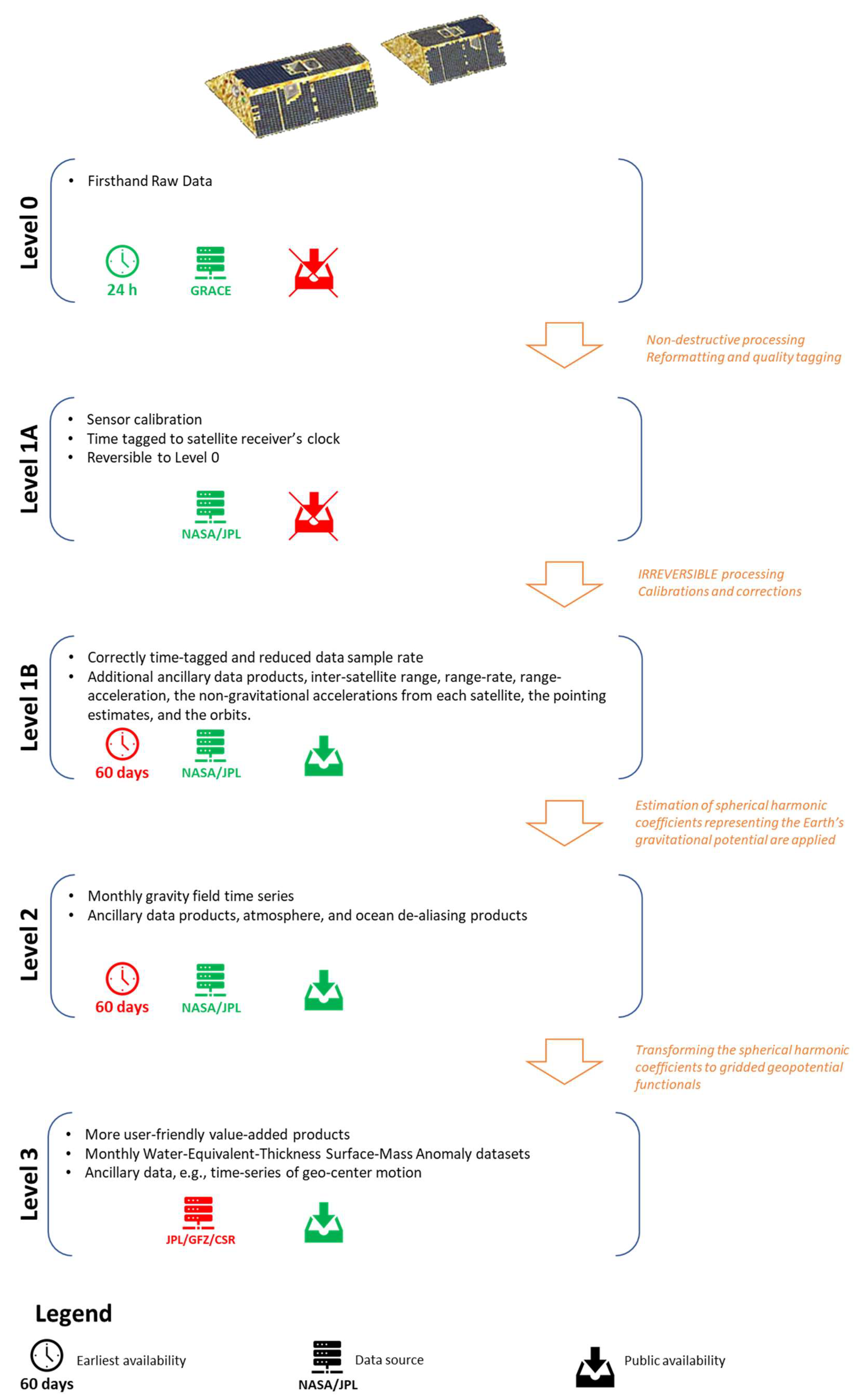
3.2.1. GRACE Products

The data obtained from the GRACE provide the information about the gravity anomalies. It needs extensive processing to extract groundwater-related direct information. The GRACE data can be classified into three stages/levels. The raw data, collected from satellites (Level 0), is calibrated and time tagged in a non-destructive (or reversible) sense and then labeled as Level 1A. Level 1A data products are not disseminated directly to the public. The data then undergo extensive and irreversible processing and are transformed to clean data products, labeled as Level 1B. These products include the inter-satellite range, range-rate, range-acceleration, the non-gravitational accelerations from each satellite, the pointing estimates, the orbits, etc. The Level 1B products are processed to produce the monthly gravity field estimates in form of spherical harmonic coefficients. These estimates are labeled Level 2. Occasionally, several months of data are combined to produce an estimate of the mean or static gravity field. After validation, all Level 2 and associated Level 1B products are released to the public.

GRACE Level 3 data represent monthly land-mass grids that possess terrestrial anomalies because of aquifers, snow covers, and river basins, etc. [94]. From the GRACE project data products, many GRACE users have put together the resources to generate and distribute value-added (or Level 3) products [95]. For the ease of users who would prefer to access GRACE data products as mass anomalies (for example water layer), some standardized products and tools are available from other sources, which are called Level 3 Data Products [96]. Figure 1 describes the GRACE data levels, processing, and the characteristics of these products.

Spherical harmonic (SH) (Level 2) and mascon (Level 3) solutions are the two main GRACE products used for the estimation of TWS. Both techniques have successfully been used in the retrieval of time-varying gravity fields from GRACE. For SH products, filtering and leakage corrections are required to reduce the noise, while no such correction is required for the mascon solutions. The capability of SH and mascon solutions to determine basin level mass variation is computed with an assessment of how the noise and errors are handled, which are inherent in GRACE solution. Although mascon solutions have an edge over the SH by avoiding leakage correction, the performance of SH for local scales is better than the mascon if corrections are applied correctly.

Leakage error is one of the many GRACE error constituents (for example, measurement and post-processing error). Generally, a leakage adjustment is needed to recover biases. The most extensively used approach is forward modeling, which uses a priori information (generally from global model simulations or in situ observations) to mimic the GRACE data processing techniques. Uncertainties of GRACE data is another main issue. Detailed analysis of uncertainties is important to achieve reliable and optimized products for obtaining TWS changes globally. For this purpose, different statistical techniques/approaches are used. For example, to enumerate uncertainties in the changes of TWS in GRACE observations, the three-cornered hat technique is in practice. Amid all other TWS change products, the BMA-based changes in TWS demonstrate the maximum consistency using with the WGHM output [97]. Empirical Orthogonal Function decomposition technique can be used to show detailed patterns of TWS variations annually and seasonally to see the long-term trends [97]. Additionally, Monte Carlo simulation framework is effective for reduction of uncertainty and improved parameter estimation while using GRACE in the calibration of Land Surface Models (LSM) parameters [22,98,99].

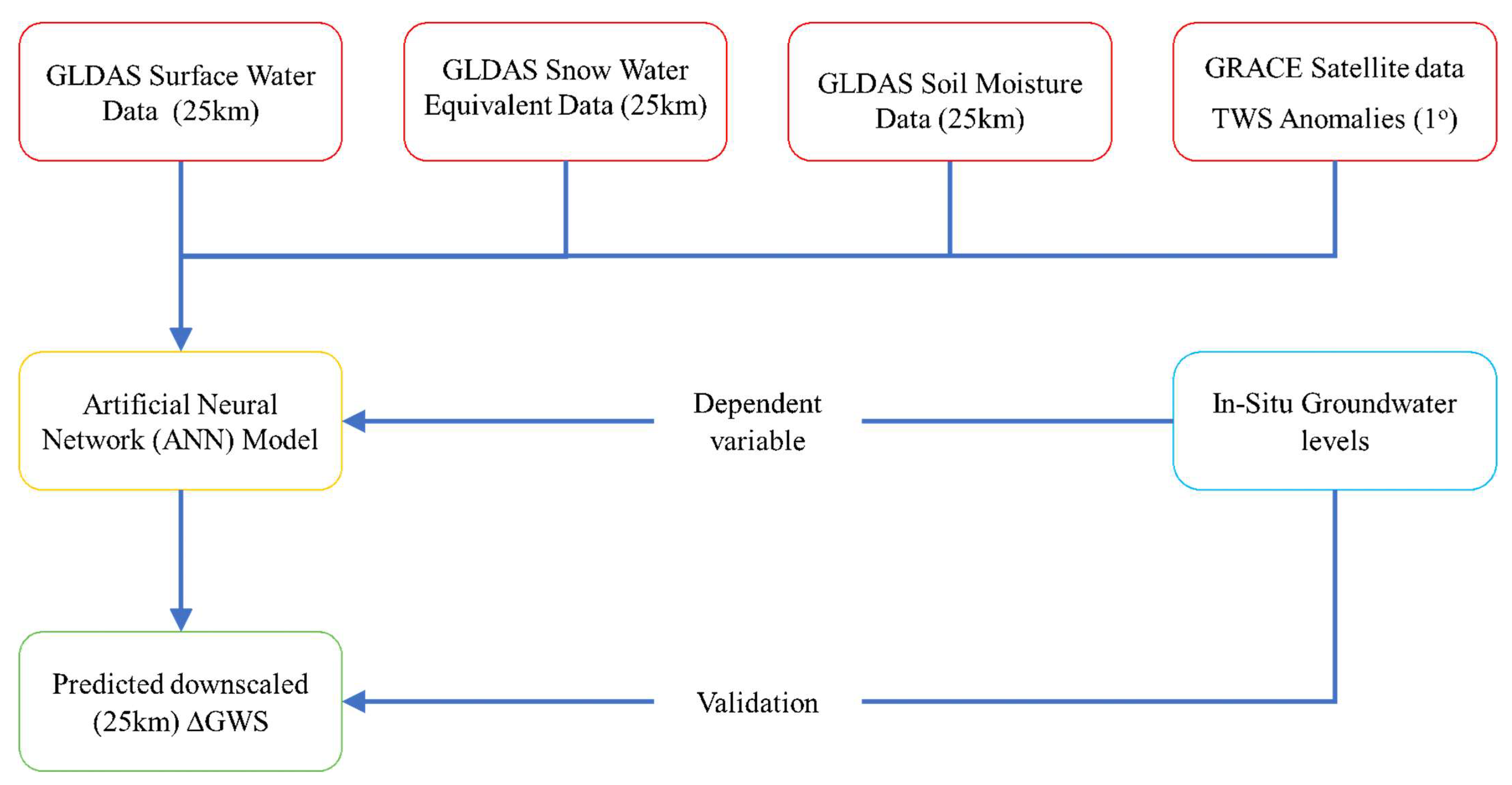
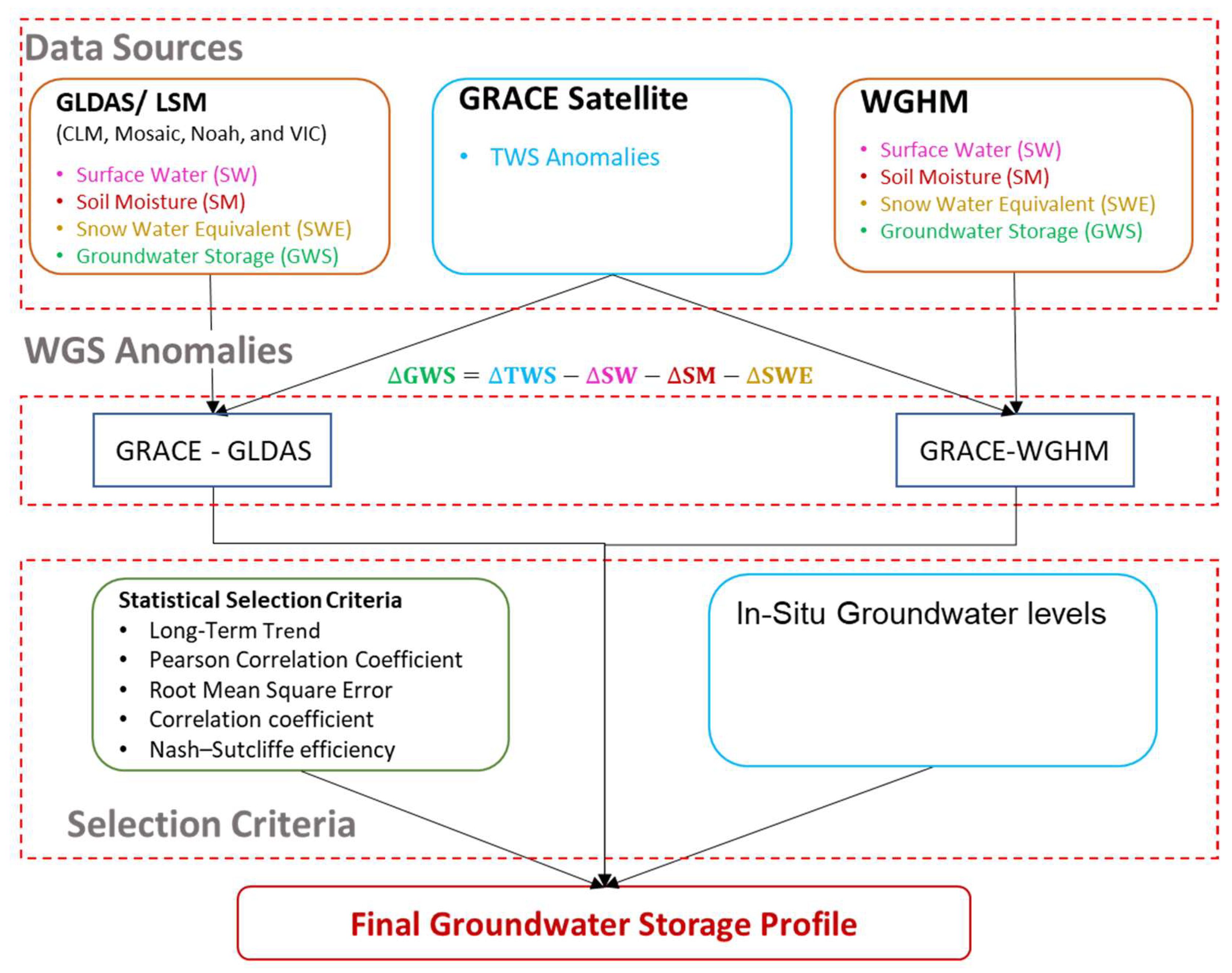
3.2.2. Estimation of Groundwater Storage (GWS)

Due to absence of long observational data and the sparse spread of monitoring wells, satellite-based observations of groundwater-storage variations through the GRACE satellite are often used to estimate the groundwater-storage changes [17,100,101]. Terrestrial water storage includes all landforms of water available to an area. It includes groundwater, surface water and canopy water, soil moisture, and snow and is a main component of the global and continental hydrologic cycle. Groundwater-storage (GWS) changes are acquired from TWS through deducting soil moisture, surface water, canopy water, and snow water equivalent data gained from GLDAS or with any other dataset [26,102,103,104]. Figure 2 explains the components of freshwater storage and processes. The same is explained in the following Equations (1) and (2):

$$\Delta TW{S}_{GRACE}=\Delta S_{groundwater}+\Delta S_{canopy}+\Delta S_{snow}+\Delta S_{soil}+\Delta S_{lakes}+\Delta S_{wetlands}+\Delta S_{river}$$

(1)

$$\Delta S_{grounwater}=\Delta \mathrm{TW}{S}_{GRACE}-\Delta S_{canopy}-\Delta S_{snow}-\Delta S_{soil}-\Delta S_{lakes}-\Delta S_{wetlands}-\Delta S_{river}$$

(2)

Since 2002, the GRACE has supplied a highly valued dataset, which allows the study of TWS over large river basins globally. Shamsudduha et al. [105] used GRACE datasets for a long time period and found that for the recent time period (2003 to 2007), groundwater-storage changes correlate well with in situ borehole records in the Bengal Basin in Bangladesh. For the Indus Basin, the variation in groundwater storage at numerous spatial scales has been studied by Iqbal et al. [106] with GRACE data. They found that the groundwater storage changes through GRACE-based estimation is reasonably sufficient for the provision of monthly groundwater-storage changes.

Variations in TWS can be acquired through the GRACE data. After the changes in groundwater, the variation of soil moisture is normally the highest factor in TWS changes and intermediate zone storage [107]. Strassberg et al. [108] found a robust link between the sum of soil moisture and groundwater storage with TWS by means of GRACE data. Before GRACE satellite, estimates of TWS changes were used to derive from the in situ data of soil moisture and snow. These approaches cover analyzing the variations in groundwater, soil water, surface water, and snow through utilizing a long time series [107].

Since the GRACE satellite was launched in 2002, a great deal of researchers has conducted the studies of groundwater using GRACE satellite data. According to the research articles published in various journals (source: https://scholar.google.com/, dated 18 January 2022), an annual frequency graph of articles has been developed to envisage the work carried out using GRACE data (refer to Figure 3).

3.2.3. GRACE Applications

GRACE provides useful information about global groundwater depletion. The shallow GWS declines faster than the deep GWS [109]. Globally, GRACE could be the only hope for the assessment of groundwater reduction [104]. GRACE data are useful for the estimation of regional groundwater monitoring on monthly to seasonal scale. Yeh et al. [110] confirmed the ability of GRACE to simulate regional groundwater-storage changes from monthly to seasonal scale for an area of about 200,000 km² area in Illinois. It also provides reasonable results for the heterogeneous GWS variations as observed by Huang et al. [109]. Döll et al. [111] conducted groundwater storage monitoring for the Mississippi Basin. However, the study failed to obtain reliable results to monitor the total water storage due to water withdrawals at the whole scale of the basin. GRACE data were applied in global hydrological investigations, including water storage change evaluation, groundwater and evapotranspiration retrieving, drought analysis, and glacier response to global change [112]. In another study, complementary relationship (CR) approach was used to assess the evapotranspiration and a water balance method to estimate the runoff and base flow in the Conterminous United States (CONUS), which demonstrates how to use it with limited parameterization and datasets [113].

There are many GRACE-based studies of groundwater that showed substantial aquifer depletion for the large regions, for example, the North China, the northwest India, the Middle East, the Murray Darling Basin of Australia, and California’s Central Valley aquifers of the USA [17,101,114,115,116,117]. The shrinking phenomena of groundwater-fed lakes have also been monitored through GRACE and GLDAS [16]. Sun et al. [118] developed a method for estimation of aquifer storage parameters (specific yield and storability) utilizing the GRACE data for the connected aquifers of Edwards-Trinity Plateau and Pecos Valley in central Texas. Frappart and Ramillien [60] also found that these data were used to evaluate the parameters; the specific yield, for example, is used to relate groundwater level to storage or to describe the indices of groundwater depletion and stress. In another GRACE-GLDAS study, it was found that high consistency exists between GRACE observations and changes in water wells [119].

3.2.4. Additional Computational Tools

For groundwater management, the usage of GRACE data at a local scale has been inadequate due to in-built uncertainties in GRACE data and problems in disintegrating several TWS components.

Artificial Neural Network (ANN) models can be developed to foresee the variations of groundwater levels directly by means of a gridded GRACE product and other openly existing hydro-meteorological datasets. ANN is used as a statistical downscaling method, which is extensively used in streamflow projecting and management of water resources [120,121,122,123,124,125,126]. A trained ANN model is comparatively strong to data noise and is quite suitable to support real-time decision making [127,128]. Ensemble ANN models can be utilized to forecast monthly and seasonal groundwater-level changes for various wells situated in certain areas.

Because of the GRACE data, the ANN models forecast water-level variations instead of absolute water levels [128]. By combining GRACE, TRMM, and GLDAS, ANN predicts and evaluates groundwater drought [129]. Gemitzi et al. [130] used ANN to perform statistical downscaling of GRACE data using local meteorological data. A typical application process of ANN is shown in Figure 4.

Srivastava and Bhattacharya integrated numerous thematic plots on the GIS platform based on Saaty’s Analytical Hierarchy Process (AHP) with the Groundwater Potential Index (GWPI) values (0.175 to 0.940) to produce a good match with the resistivity and pumping test data [92]. Similarly, AHP was used by Mallick et al. [41] to find the most important contributing features to delineate the groundwater potential zones [131].

3.3. Supporting Terrestrial Modeling Systems

To monitor the other constituents of terrestrial water storage, for example, soil water, surface water, snow and ice water, canopy water, and groundwater, separately, some system is required to address this aspect, which was fulfilled by upgrading the GRACE system. This can be done with Global Land Data Assimilation System (GLDAS) and WaterGAP Global Hydrological Model (WGHM), which help GRACE to disintegrate the TWS into its required water component. For example, TWS disintegrates with help of these models to give groundwater anomalies.

3.3.1. Global Land Data Assimilation System (GLDAS)

The Global Land Data Assimilation System (GLDAS) is a worldwide, high-resolution, offline terrestrial modeling system that integrates satellite and ground-based observations to produce optimum fields of land surface conditions and fluxes in near-real time.

It produces a sequences of worldwide land surface conditions (for example, soil moisture and surface temperature) and fluxes (for example, evaporation and sensible heat flux) products that were simulated by four Land Surface Models (LSM), that is, VIC, Mosaic, CLAM, and Noah.

Several current and proposed weather and climate prediction, water resources applications, and water-cycle investigations rely on GLDAS output. GLDAS runs globally and on user defined domains at resolutions ranging from 2.5° to 1 km. The GRACE and GLDAS simulations provide precise and reliable datasets that are used to describe the variations of groundwater storage regionally [132]. The assessed groundwater variations by GRACE-GLDAS are usually in line with in situ observations [22,97,98,109,110,132,133].

3.3.2. WaterGAP Global Hydrological Model (WGHM)

WGHM calculates timeseries of surface and subsurface runoff, groundwater recharge, and river flows along with water storage variations in canopy, snow, soil, groundwater, rivers, lakes, and wetlands. Therefore, it can quantify the whole water resources along with the groundwater resources. Institute of Physical Geography (IPG) developed WGHM to provide freshwater fluxes with storage data on the land surface globally [134,135]. The spatial resolution of the model is 0.5° × 0.5°, and computations are carried out on daily basis, whereas the output is analyzed on a monthly time step. The WGHM considers the human-induced water consumption along with the daily groundwater simulations [134]. Figure 5 explains the possible approaches to incorporated GLDAS and WGHM data to obtain GWS from the GRACE data. In this figure, it can be seen that TWS is obtained through GRACE satellite, whereas both GLDAS and WGHM give surface water, soil moisture, snow water equivalent, and groundwater storage. Final groundwater storage profiles are obtained through the interaction of GRACE with GLDAS and GRACE with WGHM, which can be compared with in situ groundwater measurements based upon the statistical selection criteria as given in the figure.

4. Regional Groundwater Estimation through Numerical Modeling

The measurement of point-based water levels eventually leads to construct the troughs and peaks of the water table. Mostly, the collected data have been too sparse to construct a credible water surface profile. Several techniques, methods, and models have been developed over time to develop accurate groundwater surface profiling. The prevailing models can be classified into three general types:

• Point-to-areal-distribution models;
• Hydrologic budget-based models;
• Commercially available software tools.

4.1. Point to areal Distribution Models

The point groundwater level values are used to get regional groundwater estimates. On the other hand, point level values in inaccessible areas can be obtained from the groundwater surface profiles. Kriging interpolation is the most widely used method. It estimates an unknown point by making use of a known point [136]. Results using kriging techniques are more efficient when data for variables are distributed normally [137]. Severely skewed distributions can often be alleviated by appropriate transformation of the data. The most common is the natural logarithmic transform, which is the best suited to lognormal data [137]. Other common methods include arithmetic average, trend analysis, regression analysis, and inverse distance method, etc.

4.2. Hydrologic Budget-Based Models

These methodologies adopted for quantifying groundwater resources are generally based on the hydrologic budget equation. The hydrologic equation for groundwater regime is a specialized form of water-balance equation that requires quantification of inflow-outflow from a groundwater reservoir as well as changes in storage therein [138]. Groundwater rise or depletion is directly calculated using calibrated groundwater models, analytical approaches, or volumetric budget analyses for multiple aquifer systems [139].

Static or steady-state modeling provides an overview of groundwater by assessing groundwater recharge by subtracting estimates of groundwater abstraction. Whereas, transient modeling is used to identify hotspots of groundwater depletion where lateral groundwater flows between the basins are significant [9].

Areas where groundwater recharge accounts for a lower fraction of total runoff are highly vulnerable to seasonal and inter-annual precipitation variability and water pollution [140]. Such areas require frequent monitoring of groundwater. To develop a reliable groundwater profile of such areas, all measurements of hydraulic head at such study sites should be made approximately at the same time, and the resulting contour and flow field maps are representative of only that specific time [141]. Monitoring of groundwater usage is not possible in real time at a global level with classical approaches. Mostly, the data of private wells are not shared in a systematic way, whereas the number of official monitoring wells are normally sparsely placed due to their high costs. Therefore, such conventional monitoring can neither be reliable nor quick.

4.3. Available Groundwater Numerical Models

Based on the geostatistical or hydrologic budget equation, many GIS-capable software tools are available to develop groundwater surface over the whole groundwater basin. For example, USGS Modular Groundwater Flow Model (MODFLOW), Finite Element Subsurface Flow System (FEFLOW) [142], Groundwater and Surface-water FLOW (GSFLOW) [143], (PHREEQC and HST3D) PHAST [144], and Saturated-Unsaturated Transport (SUTRA) are a computer programs that are used for groundwater flow modeling. They are used to simulate groundwater fluctuations, fluid movement, and the transport of dissolved substances in a subsurface environment.

Finite Element Subsurface FLOW System (FEFLOW) is a groundwater model developed by Danish Hydraulic Institute (DHI). The program uses finite element analysis to solve the groundwater flow equation of both saturated and unsaturated conditions and can reasonably provide a good model of the hydraulic heads [145].

Another model is the semi-coupled SWAT-MODFLOW model (SWATmf) [146], used to assess the future patterns of streamflow, groundwater levels, and reservoir storage from three management practices under the most aggressive climatic scenario (RCP8.5) at the Fort Cobb Reservoir Experimental Watershed (FCREW); it was developed by Triana et al. [147].

Free and open-source applications, such as ModelMuse [148] and FREEWAT [149], are the effective supporting tools used for groundwater modeling. Spatial data management and numerical modeling demonstrate the application of the QGIS-Integrated FREEWAT platform in 13 case studies for tackling groundwater resource management.

5. Conclusions and Recommendations

The conventional monitoring of groundwater largely depends upon the site measurement/model simulations, which is expensive and timewasting. Moreover, during the conversion from observation points to large areas, added error is brought into spatially constant data acquired by statistical interpolation techniques. The accuracy of interpolation outcomes may considerably drop in areas far away from observation sites. Additionally, some of the extrapolation methods are generally insufficient and biased; they do not provide enough information about the variance of the estimations. While conventional monitoring methods provide the point measurement and are more accurate as compared to satellite-based observations, the time, cost, and labor involved is sometimes not affordable.

Groundwater-related hydrological studies have become more useful and economical with the start of numerous satellite imageries and numerical modeling.

The extensive use of satellite data ensures a robust and cost-effective estimation of groundwater-storage variations. Inclusion of satellite data for groundwater monitoring is a remarkable milestone in the field of groundwater management. It enables policymakers to manage water resources on a real-time basis.

Specifically, the use of satellite data in groundwater resources accelerated very rapidly with the launching of GRACE satellite. GRACE satellite data are mostly utilized to assess the groundwater-storage changes. This satellite covers the issue of cost, time, and labor by providing its free data for some areas/regions, which can be used to assess groundwater evaluation efficiently at a global, regional, or national level. Combinations of other satellite products, computational tools, GIS techniques, and hydro-climate models have proved most effective so far. Different other models, such as GLDAS and WGHM, are efficient tools that are very helpful to use in integration with GRACE through upgrading its resolution.

Numerical modeling can also a useful tool for the simulation of groundwater resources for some areas and projects in the future. Therefore, GRACE and groundwater modeling can be tested to be used conjunctively for better evaluation of groundwater resources for a region.

Significant research has been conducted to increase the accuracy of the satellite-based groundwater estimates. However, dependency on point-based measurements has not been overruled. Point-based measurements are still considered most accurate and reliable method for the calibration of satellite and modeling data. A strategic usage of satellite-based models with point-measurement investigations would prominently improve the knowledge base of policymakers. A focus on point-based measurement is required with the help of cost-effective, robust, and accurate detection of groundwater levels using latest technologies.

References

1. Environmental Literacy Teacher Guide Series: Earth’s Freash Water. 2019. Available online: https://media.nationalgeographic.org/assets/file/freshwater_chapter6_v2.pdf (accessed on 10 September 2021).
2. de Gramont, H.M.; Noel, C.; Oliver, J.L.; Pennequin, D.; Rama, M.; Stephan, R.M.; Frouin, K. Towards a Joint Management of Transboundary Aquifer Systems; A Savoir 03; AFD Research Department: Paris, Frence, 2011. [Google Scholar]
3. Siebert, S.; Burke, J.; Faures, J.M.; Frenken, K.; Hoogeveen, J.; Döll, P.; Portmann, F.T. Groundwater use for irrigation—A global inventory. Hydrol. Earth Syst. Sci. 2010, 14, 1863–1880. [Google Scholar] [CrossRef] [Green Version]
4. Wada, Y.; van Beek, L.P.H.; van Kempen, C.M.; Reckman, J.W.T.M.; Vasak, S.; Bierkens, M.F.P. Global depletion of groundwater resources. Geophys. Res. Lett. 2010, 37, L20402. [Google Scholar] [CrossRef] [Green Version]
5. Moench, M.; Burke, J.; Moench, Y. Rethinking the Approach to Groundwater and Food Security; FAO: Rome, Italy, 2003. [Google Scholar]
6. Kløve, B.; Ala-aho, P.; Bertrand, G.; Boukalova, Z.; Ertürk, A.; Goldscheider, N.; Ilmonen, J.; Karakaya, N.; Kupfersberger, H.; Kvœrner, J.; et al. Groundwater dependent ecosystems. Part I: Hydroecological status and trends. Environ. wSci. Policy 2011, 14, 770–781. [Google Scholar] [CrossRef]
7. Gupta, J.; Pahl-Wostl, C.; Zondervan, R. “Glocal” water governance: A multi-level challenge in the anthropocene. Curr. Opin. Environ. Sustain. 2013, 5, 573–580. [Google Scholar] [CrossRef]
8. Lopez-Gunn, E.; Llamas, M.R. Re-thinking water scarcity: Can science and technology solve the global water crisis? Nat. Resour. Forum. 2008, 32, 228–238. [Google Scholar] [CrossRef]
9. de Graaf, I.E.M.; van Beek, R.L.P.H.; Gleeson, T.; Moosdorf, N.; Schmitz, O.; Sutanudjaja, E.H.; Bierkens, M.F.P. A global-scale two-layer transient groundwater model: Development and application to groundwater depletion. Adv. Water Resour. 2017, 102, 53–67. [Google Scholar] [CrossRef]
10. Kløve, B.; Ala-Aho, P.; Bertrand, G.; Gurdak, J.J.; Kupfersberger, H.; Kværner, J.; Muotka, T.; Mykrä, H.; Preda, E.; Rossi, P.; et al. Climate change impacts on groundwater and dependent ecosystems. J. Hydrol. 2014, 518, 250–266. [Google Scholar] [CrossRef]
11. Green, T.R.; Taniguchi, M.; Kooi, H.; Gurdak, J.J.; Allen, D.M.; Hiscock, K.M.; Treidel, H.; Aureli, A. Beneath the surface of global change: Impacts of climate change on groundwater. J. Hydrol. 2011, 405, 532–560. [Google Scholar] [CrossRef] [Green Version]
12. Famiglietti, J.S. The global groundwater crisis. Nat. Clim. Chang. 2014, 4, 945–948. [Google Scholar] [CrossRef]
13. Gleeson, T.; VanderSteen, J.; Sophocleous, M.A.; Taniguchi, M.; Alley, W.M.; Allen, D.M.; Zhou, Y. Groundwater sustainability strategies. Nat. Geosci. 2010, 3, 378–379. [Google Scholar] [CrossRef]
14. Gleeson, T.; Wada, Y.; Bierkens, M.F.P.; Van Beek, L.P.H. Water balance of global aquifers revealed by groundwater footprint. Nature 2012, 488, 197–200. [Google Scholar] [CrossRef] [PubMed]
15. Giordano, M. Global groundwater? Issues and solutions. Annu. Rev. Environ. Resour. 2009, 34, 153–178. [Google Scholar] [CrossRef]
16. Jiao, J.J.; Zhang, X.; Wang, X. Satellite-based estimates of groundwater depletion in the Badain Jaran Desert, China. Sci. Rep. 2015, 5, 8960. [Google Scholar] [CrossRef] [PubMed] [Green Version]
17. Rodell, M.; Velicogna, I.; Famiglietti, J.S. Satellite-based estimates of groundwater depletion in India. Nature 2009, 460, 999–1002. [Google Scholar] [CrossRef] [PubMed] [Green Version]
18. Aeschbach-Hertig, W.; Gleeson, T. Regional strategies for the accelerating global problem of groundwater depletion. Nat. Geosci. 2012, 5, 853–861. [Google Scholar] [CrossRef]
19. IAEA. Isotope Methods for Dating Old Groundwater; IAEA: Vienna, Austria, 2013. [Google Scholar]
20. Khan, H.F.; Ethan Yang, Y.C.; Ringler, C.; Wi, S.; Cheema, M.J.M.; Basharat, M. Guiding groundwater policy in the indus basin of Pakistan using a physically based groundwater model. J. Water Resour. Plan. Manag. 2017, 143, 05016014. [Google Scholar] [CrossRef]
21. Kaika, M. The Water Framework Directive: A New Directive for a Changing Social, Political and Economic European Framework. Eur. Plan. Stud. 2003, 11, 303. [Google Scholar] [CrossRef]
22. Voss, K.A.; Famiglietti, J.S.; Lo, M.; de Linage, C.; Rodell, M.; Swenson, S.C. Groundwater depletion in the Middle East from GRACE with implications for transboundary water management in the Tigris-Euphrates-Western Iran region. Water Resour. Res. 2013, 49, 904–914. [Google Scholar] [CrossRef] [Green Version]
23. Jelovčan, M.; Šraj, M. Analysis of groundwater levels in piezometers in the vipava valley. Acta Hydrotech. 2020, 33, 61–78. [Google Scholar] [CrossRef]
24. Bonacci, E.O.; Roje-Bonacci, E.T. Analysis of groundwater levels and lake vrana water levels on the cres Island. Hrvat. Vode 2018, 26, 39–47. [Google Scholar]
25. Sattari, M.T.; Mirabbasi, R.; Sushab, R.S.; Abraham, J. Prediction of Groundwater Level in Ardebil Plain Using Support Vector Regression and M5 Tree Model. Groundwater 2018, 56, 636–646. [Google Scholar] [CrossRef] [PubMed]
26. Yin, W.; Hu, L.; Jiao, J.J. Evaluation of Groundwater Storage Variations in Northern China Using GRACE Data. Geofluids 2017, 2017, 8254824. [Google Scholar] [CrossRef] [Green Version]
27. Novakovic, B.; Farvolden, R.N. Investigations of Groundwater Flow Systems in Big Creek and Big Otter Creek Drainage Basins, Ontario. Can. J. Earth Sci. 1974, 11, 964–975. [Google Scholar] [CrossRef]
28. Husain, M.M.; Cherry, J.A.; Fidler, S.; Frape, S.K. On the long-term hydraulic gradient in the thick clayey aquitard in the Sarnia region, Ontario. Can. Geotech. J. 1998, 35, 986–1003. [Google Scholar] [CrossRef]
29. Groundwater Monitoring Procedures for Operation and Maintenance Norms. 2002. Available online: https://www.google.com/url?sa=t&rct=j&q=&esrc=s&source=web&cd=&cad=rja&uact=8&ved=2ahUKEwiJs4qWl_z1AhWesVYBHWlVBhcQFnoECAMQAQ&url=http%3A%2F%2Fhydrology-project.gov.in%2FPDF%2F-download-manuals-General-HPIIfollow-upWorkingDraftPaper.pdf&usg=AOvVaw2KZyJ646-2EQ-CqBL1ci56 (accessed on 10 September 2021).
30. Cunningham, W.L.; Schalk, C.W. Groundwater Technical Procedures of the U.S. Geological Survey. Available online: https://pubs.usgs.gov/tm/1a1/pdf/tm1-a1.pdf (accessed on 10 September 2021).
31. Peralta, R.C.; Mazur, V.; Dutram, P. Monitoring of Groundwater Levels for Real-Time Conjunctive Water Management. Publ.—Arkansas Water Resour. Res. Cent. 1983, 92, 1–27. [Google Scholar]
32. Authority, S.G. Groundwater Level Monitoring Plan for the Sacramento Groundwater Authority CASGEM Well Network. 2011. Available online: https://www.sgah2o.org/wp-content/uploads/2016/06/pub-CASGEM-Plan-12-21-11.pdf (accessed on 10 September 2021).
33. Garber, M.S.; Koopman, F.C. Methods of Measuring Water Levels in Deep Wells. Available online: https://pubs.er.usgs.gov/publication/twri08A1 (accessed on 10 September 2021).
34. Chevalking, L.K.; van Steenbergen Description, F. Ideas for Groundwater Management. Available online: https://metameta.nl/wp-content/uploads/2010/05/Ideas_for_Groundwater_Management_Digital.pdf (accessed on 15 November 2021).
35. Cunningham, W.L.; Schalk, C.W. Groundwater technical procedures of the U.S. Geological Survey: U.S. Geological Survey Techniques and Methods 1–A1, 151 p, GWPD 16-Measuring water levels in wells and piezometers by use of a submersible pressure transducer. In Groundwater technical procedures of the U.S. Geological Survey; 2010; pp. 139–144. Available online: https://pubs.usgs.gov/tm/1a1/ (accessed on 10 September 2021).
36. Kalbus, E.; Reinstorf, F.; Schirmer, M. Hydrology and Earth System Sciences Measuring Methods for Groundwater-Surface Water Interactions: A Review. Hydrol. Earth Syst. Sci. 2006, 10, 873–887. [Google Scholar] [CrossRef] [Green Version]
37. Gray Member, D.M.; Mahapatra, A.K. A Method of Measurement of the Ground Water Table and Soil Hydraulic Conductivity; Canadian Agriculture Engineering Department, University of Saskatchewan Saskatoon: Saskatoon, SK, Canada, 1965; Volume 7, pp. 25–27, 36. Available online: https://library.csbe-scgab.ca/docs/journal/7/7_1_25_ocr.pdf (accessed on 10 September 2021).
38. Freeman, L.A.; Carpenter, M.C.; Rosenberry, D.O.; Rousseau, J.P.; Unger, R.; McLean, J.S. Use of Submersible Pressure Transducers in Water-Resources Investigations. 2004, pp. 1–65. Available online: https://www.mendeley.com/catalogue/7e74894e-5a41-3358-bc1d-455c09fec44d/ (accessed on 6 January 2022).
39. Rossetto, R.; Barbagli, A.; Borsi, I.; Mazzanti, G.; Vienken, T.; Bonari, E. Site investigation and design of the monitoring system at the Sant’Alessio Induced RiverBank Filtration plant (Lucca, Italy). Rend. Online Soc. Geol. Ital. 2015, 35, 248–251. [Google Scholar] [CrossRef]
40. Rosenberry, D.O.; Labaugh, J.W.; Hunt, R.J. Use of Monitoring Wells, Portable Piezometers, and Seepage Meters to Quantify Flow between Surface Water and Ground Water Chapter 2 of Field Techniques for Estimating Water Fluxes between Surface Water and Ground Water, U.S Geological Survey. Techniques and Methods Chapter 4-D2; 2008; pp. 39–90. Available online: https://pubs.usgs.gov/tm/04d02/pdf/TM4-D2-chap2.pdf (accessed on 10 September 2021).
41. Mallick, J.; Singh, C.K.; Al-Wadi, H.; Ahmed, M.; Rahman, A.; Shashtri, S.; Mukherjee, S. Geospatial and geostatistical approach for groundwater potential zone delineation. Hydrol. Process. 2015, 29, 395–418. [Google Scholar] [CrossRef]
42. García-Menéndez, O.; Ballesteros, B.J.; Renau-Pruñonosa, A.; Morell, I.; Mochales, T.; Ibarra, P.I.; Rubio, F.M. Using electrical resistivity tomography to assess the effectiveness of managed aquifer recharge in a salinized coastal aquifer. Environ. Monit. Assess. 2018, 190, 100. [Google Scholar] [CrossRef]
43. Mohamaden, M.I.I. Electric resistivity investigation at Nuweiba Harbour Gulf of Aqaba, South Sinai, Egypt. Cit. Egypt. J. Aquat. Res. 2005, 31, 58–67. [Google Scholar]
44. Mohamaden, M.I.I. Groundwater exploration at Rafah, Sinai Peninsula, Egypt. Egypt. J. Aquat. Res. 2008, 35, 49–68. [Google Scholar]
45. Shagar, M.M.S.A. Structural effect on the groundwater at the Arish City, North eastern Part of Sinai Peninsula, Egypt Egypt. Egypt. J. Aquat. Res. 2008, 35, 31–47. [Google Scholar]
46. Mohamaden, M.I.I.; Wahaballa, A.; El-Sayed, H.M. Application of electrical resistivity prospecting in waste water management: A case study Kharga Oasis, Egypt. Egypt. J. Aquat. Res. 2016, 42, 33–39. [Google Scholar] [CrossRef] [Green Version]
47. Mohamaden, M.I.I.; Ehab, D. Application of electrical resistivity for groundwater exploration in Wadi Rahaba, Shalateen, Egypt. NRIAG J. Astron. Geophys. 2017, 6, 201–209. [Google Scholar] [CrossRef]
48. Raji, W.O. Review of Electrical and Gravity Methods of Near-Surface Exploration for Groundwater. Niger. J. Technol. Dev. 2014, 11, 31–38. [Google Scholar]
49. Rolia, E.; Sutjiningsih, D. Application of Geoelectric Method for Groundwater Exploration from Surface (A Literature Study); American Institute of Physics: New York, NY, USA, 1977; p. 20018. [Google Scholar] [CrossRef]
50. Rosid, M.S.; Kepic, A.W. Hydrogeological mapping using the Seismoelectric Method. Explor. Geophys. 2005, 36, 245–249. [Google Scholar] [CrossRef]
51. Britannica. Earth Exploration—Seismic Refraction Methods|Britannica. Available online: https://www.britannica.com/topic/Earth-exploration/Seismic-refraction-methods (accessed on 6 January 2022).
52. Chandler, V.M. Gravity Investigation for Potential Ground-Water Resources in Rock County, Minnesota; Report of Investigations 44; University of Minnesota: St. Paul, MN, USA, 1994; ISSN 0076-9177. Available online: https://conservancy.umn.edu/bitstream/handle/11299/60798/1/mgs-264.pdf (accessed on 15 September 2021).
53. Sabri, L.M.; Sudarsono, B.; Aryadi, Y. Groundwater Change Detection by Gravity Measurement on Northern Coast of Java: A Case Study in Semarang City of Central Java of Indonesia. Available online: https://iopscience.iop.org/article/10.1088/1757-899X/797/1/012032 (accessed on 6 January 2022).
54. Davis, K.; Li, Y.; Batzle, M. Time-lapse gravity monitoring: A systematic 4D approach with application to aquifer storage and recovery. Geophysics 2008, 73, WA61–WA69. [Google Scholar] [CrossRef]
55. Iqbal, N.; Ashraf, M.; Imran, M.; Salam, H.A.; Hasan, F.U.; Khan, A.D. Groundwater Investigations and Mapping in the Lower Indus Plain; PCRWR: Islamabad, Pakistan, 2020. [Google Scholar]
56. Kendall, C.; Aravena, R. Nitrate Isotopes in Groundwater Systems. In Environmental Tracers in Subsurface Hydrology; Springer: Boston, MA, USA, 2000; pp. 261–297. [Google Scholar]
57. Balkhair, K.S.; Masood, A.; Almazroui, M.; Rahman, K.U.; Bamaga, O.A.; Kamis, A.S.; Ahmed, I.; Al-Zahrani, M.I.; Hesham, K. Groundwater share quantification through flood hydrographs simulation using two temporal rainfall distributions. Desalin. Water Treat. 2018, 114, 109–119. [Google Scholar] [CrossRef] [Green Version]
58. Chen, J.L.; Wilson, C.R.; Tapley, B.D.; Scanlon, B.; Güntner, A. Long-term groundwater storage change in Victoria, Australia from satellite gravity and in situ observations. Glob. Planet. Chang. 2016, 139, 56–65. [Google Scholar] [CrossRef] [Green Version]
59. Oikonomidis, D.; Dimogianni, S.; Kazakis, N.; Voudouris, K. A GIS/Remote Sensing-based methodology for groundwater potentiality assessment in Tirnavos area, Greece. J. Hydrol. 2015, 525, 197–208. [Google Scholar] [CrossRef]
60. Frappart, F.; Ramillien, G. Monitoring groundwater storage changes using the Gravity Recovery and Climate Experiment (GRACE) satellite mission: A review. Remote Sens. 2018, 10, 829. [Google Scholar] [CrossRef] [Green Version]
61. Rohith, G.; Sutha Kumar, L.; Purnamasayangsukasih, R.P.; Adnan, M.I.A. A review of uses of satellite imagery in monitoring mangrove forests. IOP Conf. Ser. Earth Environ. Sci. 2016. [Google Scholar] [CrossRef]
62. WMO. The Global Satellite Observing System: A Success Story|World Meteorological Organization. 2010. Available online: https://public.wmo.int/en/bulletin/global-satellite-observing-system-success-story (accessed on 8 January 2022).
63. Elbeih, S.F. An overview of integrated remote sensing and GIS for groundwater mapping in Egypt. Ain Shams Eng. J. 2015, 6, 1–15. [Google Scholar] [CrossRef] [Green Version]
64. Nayak, T.R.; Gupta, S.K.; Galkate, R. GIS Based Mapping of Groundwater Fluctuations in Bina Basin. Aquat. Procedia 2015, 4, 1469–1476. [Google Scholar] [CrossRef]
65. Nouri, H.; Nagler, P.; Chavoshi Borujeni, S.; Barreto Munez, A.; Alaghmand, S.; Noori, B.; Galindo, A.; Didan, K. Effect of spatial resolution of satellite images on estimating the greenness and evapotranspiration of urban green spaces. Hydrol. Process. 2020, 34, 3183–3199. [Google Scholar] [CrossRef]
66. Huete, A.; Didan, K.; Miura, T.; Rodriguez, E.P.; Gao, X.; Ferreira, L.G. Overview of the radiometric and biophysical performance of the MODIS vegetation indices. Remote Sens. Environ. 2002, 83, 195–213. [Google Scholar] [CrossRef]
67. NASA-MODIS. 2020. Available online: https://earthdata.nasa.gov/earth-observation-data/near-real-time/download-nrt-data/modis-nrt (accessed on 25 September 2021).
68. Masood, A.; Mushtaq, H. Spatio-Temporal Analysis of Early Twenty-First Century Areal Changes in the Kabul River Basin Cryosphere. Earth Syst. Environ. 2018, 2, 563–571. [Google Scholar] [CrossRef]
69. Hashmi, M.Z.U.R.; Masood, A.; Mushtaq, H.; Bukhari, S.A.A.; Ahmad, B.; Tahir, A.A. Exploring climate change impacts during first half of the 21st century on flow regime of the transboundary kabul river in the hindukush region. J. Water Clim. Chang. 2020, 11, 1521–1538. [Google Scholar] [CrossRef]
70. Zhang, Z.; Moore, J.C. Mathematical and Physical Fundamentals of Climate Change. Available online: https://www.elsevier.com/books/mathematical-and-physical-fundamentals-of-climate-change/zhang/978-0-12-800066-3 (accessed on 25 September 2021). eBook ISBN: 97801280058352014.
71. Cao, Z. Assessment methods for air pollution exposure. In Spatiotemporal Analysis of Air Pollution and Its Application in Public Health; Elsevier: Amsterdam, The Netherlands, 2020; pp. 197–206. [Google Scholar] [CrossRef]
72. Westerhoff, R.; White, P.; Rawlinson, Z. Application of global models and satellite data for smaller-scale groundwater recharge studies. Hydrol. Earth Syst. Sci. 2016. [Google Scholar] [CrossRef] [Green Version]
73. Elmahdy, S.; Mohamed, M.; Ali, T. Land use/land cover changes impact on groundwater level and quality in the northern part of the United Arab Emirates. Remote Sens. 2020, 12, 1715. [Google Scholar] [CrossRef]
74. USGS. What Is the Landsat Satellite Program and Why Is It Important?|U.S. Geological Survey. Available online: https://www.usgs.gov/faqs/what-landsat-satellite-program-and-why-it-important (accessed on 6 January 2022).
75. Meyers, Z.P.; Frisbee, M.D.; Rademacher, L.K.; Stewart-Maddox, N.S. Old groundwater buffers the effects of a major drought in groundwater-dependent ecosystems of the eastern Sierra Nevada (CA). Environ. Res. Lett. 2021, 16, 044044. [Google Scholar] [CrossRef]
76. Sharma, A.K.; Hubert-Moy, L.; Buvaneshwari, S.; Sekhar, M.; Ruiz, L.; Bandyopadhyay, S.; Corgne, S. Irrigation history estimation using multitemporal landsat satellite images: Application to an intensive groundwater irrigated agricultural watershed in India. Remote Sens. 2018, 10, 893. [Google Scholar] [CrossRef] [Green Version]
77. Huntington, J.; McGwire, K.; Morton, C.; Snyder, K.; Peterson, S.; Erickson, T.; Niswonger, R.; Carroll, R.; Smith, G.; Allen, R. Assessing the role of climate and resource management on groundwater dependent ecosystem changes in arid environments with the Landsat archive. Remote Sens. Environ. 2016, 185, 186–197. [Google Scholar] [CrossRef] [Green Version]
78. Singh, R.K.; Khand, K.; Kagone, S.; Schauer, M.; Senay, G.B.; Wu, Z. A novel approach for next generation water-use mapping using Landsat and Sentinel-2 satellite data. Hydrol. Sci. J. 2020, 65, 2508–2519. [Google Scholar] [CrossRef]
79. Battude, M.; Al Bitar, A.; Morin, D.; Cros, J.; Huc, M.; Marais Sicre, C.; Le Dantec, V.; Demarez, V. Estimating maize biomass and yield over large areas using high spatial and temporal resolution Sentinel-2 like remote sensing data. Remote Sens. Environ. 2016, 184, 668–681. [Google Scholar] [CrossRef]
80. Clark, M.L. Comparison of simulated hyperspectral HyspIRI and multispectral Landsat 8 and Sentinel-2 imagery for multi-seasonal, regional land-cover mapping. Remote Sens. Environ. 2017, 200, 311–325. [Google Scholar] [CrossRef]
81. Ferrant, S.; Selles, A.; Le Page, M.; Herrault, P.A.; Pelletier, C.; Al-Bitar, A.; Mermoz, S.; Gascoin, S.; Bouvet, A.; Saqalli, M.; et al. Detection of irrigated crops from Sentinel-1 and Sentinel-2 data to estimate seasonal groundwater use in South India. Remote Sens. 2017, 9, 1119. [Google Scholar] [CrossRef] [Green Version]
82. Sadeghi, M.; Babaeian, E.; Tuller, M.; Jones, S.B. The optical trapezoid model: A novel approach to remote sensing of soil moisture applied to Sentinel-2 and Landsat-8 observations. Remote Sens. Environ. 2017, 198, 52–68. [Google Scholar] [CrossRef] [Green Version]
83. Campos-Taberner, M.; García-Haro, F.J.; Busetto, L.; Ranghetti, L.; Martínez, B.; Gilabert, M.A.; Camps-Valls, G.; Camacho, F.; Boschetti, M. A critical comparison of remote sensing Leaf Area Index estimates over rice-cultivated areas: From Sentinel-2 and Landsat-7/8 to MODIS, GEOV1 and EUMETSAT polar system. Remote Sens. 2018, 10, 763. [Google Scholar] [CrossRef] [Green Version]
84. Rozenstein, O.; Haymann, N.; Kaplan, G.; Tanny, J. Estimating cotton water consumption using a time series of Sentinel-2 imagery. Agric. Water Manag. 2018, 207, 44–52. [Google Scholar] [CrossRef]
85. Wang, Q.; Atkinson, P.M. Spatio-temporal fusion for daily Sentinel-2 images. Remote Sens. Environ. 2018, 204, 31–42. [Google Scholar] [CrossRef] [Green Version]
86. Eo Portal Directory. Copernicus: Sentinel-2—Satellite Missions—eoPortal Directory. Available online: https://earth.esa.int/web/eoportal/satellite-missions/c-missions/copernicus-sentinel-2 (accessed on 7 January 2022).
87. Dubois, C.; Stoffner, F.; Kalia, A.C.; Sandner, M.; Labiadh, M.; Mimouni, M. Copernicus sentinel-2 data for the determination of groundwater withdrawal in the maghreb region. In Proceedings of the ISPRS Annals of the Photogrammetry, Remote Sensing and Spatial Information Sciences IV-1, Karlsruhe, Germany, 10–12 October 2018; Volume 4, pp. 37–44. [Google Scholar]
88. Stoffner, F.; Mimouni, M. Application of sentinel 2 satellite imagery for sustainable groundwater management in agricultural areas—chtouka aquifer, morocco. Quaternary 2021, 4, 35. [Google Scholar] [CrossRef]
89. Galloway, D.L.; Jones, D.R.; Ingebritsen, S.E. Measuring Land Subsidence from Space; U.S. Geological Survey Fact Sheet 051–00; 2000; p. 4. Available online: http://pubs.usgs.gov/fs/fs-051-00/ (accessed on 30 November 2021).
90. Lu, Y.Y.; Ke, C.Q.; Jiang, H.J.; Chen, D.L. Monitoring urban land surface deformation (2004–2010) from InSAR, groundwater and levelling data: A case study of Changzhou city, China. J. Earth Syst. Sci. 2019, 128, 159. [Google Scholar] [CrossRef] [Green Version]
91. Castellazzi, P.; Schmid, W. Interpreting C-band InSAR ground deformation data for large-scale groundwater management in Australia. J. Hydrol. Reg. Stud. 2021, 34, 100774. [Google Scholar] [CrossRef]
92. Srivastava, P.K.; Bhattacharya, A.K. Groundwater assessment through an integrated approach using remote sensing, GIS and resistivity techniques: A case study from a hard rock terrain. Int. J. Remote Sens. 2006, 27, 4599–4620. [Google Scholar] [CrossRef]
93. Famiglietti, J.S.; Rodell, M. Water in the balance. Science 2013, 340, 1300–1301. [Google Scholar] [CrossRef] [PubMed]
94. Hossain, A.A. Groundwater Depletion in the Mississippi Delta as Observed by the Gravity Recovery and Climate Experiment (GRACE) Satellite System. In Proceedings of the Mississippi Water Resources Conference, Jackson, MS, USA, 24–25 April 2014; pp. 59–65. Available online: https://www.wrri.msstate.edu/pdf/2014_wrri_proceedings.pdf (accessed on 1 October 2021).
95. Landerer, F.W.; Swenson, S.C. Accuracy of scaled GRACE terrestrial water storage estimates. Water Resour. Res. 2012, 48, 1–11. [Google Scholar] [CrossRef]
96. Strugarek, D.; Sosnica, K.; Arnold, D.; J’ggi, A.; Zajdel, R.; Bury, G.; Drozdzewski, M. Determination of global geodetic parameters using satellite laser ranging measurements to sentinel-3 satellites. Remote Sens. 2019, 11, 2282. [Google Scholar] [CrossRef] [Green Version]
97. Long, D.; Pan, Y.; Zhou, J.; Chen, Y.; Hou, X.; Hong, Y.; Scanlon, B.R.; Longuevergne, L. Global analysis of spatiotemporal variability in merged total water storage changes using multiple GRACE products and global hydrological models. Remote Sens. Environ. 2017, 192, 198–216. [Google Scholar] [CrossRef]
98. Alley, W.M.; Konikow, L.F. Bringing GRACE Down to Earth. Groundwater 2015, 53, 826–829. [Google Scholar] [CrossRef]
99. Lo, M.H.; Famiglietti, J.S.; Yeh, P.J.F.; Syed, T.H. Improving parameter estimation and water table depth simulation in a land surface model using GRACE water storage and estimated base flow data. Water Resour. Res. 2010, 46, 1–15. [Google Scholar] [CrossRef]
100. Bhanja, S.N.; Mukherjee, A.; Rodell, M. Groundwater Storage Variations in India; Springer: Singapore, 2018; pp. 49–59. [Google Scholar]
101. Ahmed, K.; Shahid, S.; Demirel, M.C.; Nawaz, N.; Khan, N. The changing characteristics of groundwater sustainability in Pakistan from 2002 to 2016. Hydrogeol. J. 2019, 27, 2485–2496. [Google Scholar] [CrossRef]
102. Feng, W.; Zhong, M.; Lemoine, J.M.; Biancale, R.; Hsu, H.T.; Xia, J. Evaluation of groundwater depletion in North China using the Gravity Recovery and Climate Experiment (GRACE) data and ground-based measurements. Water Resour. Res. 2013, 49, 2110–2118. [Google Scholar] [CrossRef]
103. Castellazzi, P.; Martel, R.; Rivera, A.; Huang, J.; Pavlic, G.; Calderhead, A.I.; Chaussard, E.; Garfias, J.; Salas, J. Groundwater depletion in Central Mexico: Use of GRACE and InSAR to support water resources management. Water Resour. Res. 2016, 52, 5985–6003. [Google Scholar] [CrossRef]
104. Rodell, M.; Chen, J.; Kato, H.; Famiglietti, J.S.; Nigro, J.; Wilson, C.R. Estimating groundwater storage changes in the Mississippi River basin (USA) using GRACE. Hydrogeol. J. 2007, 15, 159–166. [Google Scholar] [CrossRef] [Green Version]
105. Shamsudduha, M.; Taylor, R.G.; Longuevergne, L. Monitoring groundwater storage changes in the highly seasonal humid tropics: Validation of GRACE measurements in the Bengal Basin. Water Resour. Res. 2012, 48, 1–12. [Google Scholar] [CrossRef] [Green Version]
106. Iqbal, N.; Hossain, F.; Lee, H.; Akhter, G. Satellite Gravimetric Estimation of Groundwater Storage Variations over Indus Basin in Pakistan. IEEE J. Sel. Top. Appl. Earth Obs. Remote Sens. 2016, 9, 3524–3534. [Google Scholar] [CrossRef]
107. Rodell, M.; Famiglietti, J.S. An analysis of terrestrial water storage variations in Illinois with implications for the Gravity Recovery and Climate Experiment (GRACE). Water Resour. Res. 2001, 37, 1327–1339. [Google Scholar] [CrossRef] [Green Version]
108. Strassberg, G.; Scanlon, B.R.; Chambers, D. Evaluation of groundwater storage monitoring with the GRACE satellite: Case study of the High Plains aquifer, central United States. Water Resour. Res. 2009, 45, 1–10. [Google Scholar] [CrossRef] [Green Version]
109. Huang, Z.; Pan, Y.; Gong, H.; Yeh, P.J.-F.; Li, X.; Zhou, D.; Zhao, W. Subregional-scale groundwater depletion detected by GRACE for both shallow and deep aquifers in North China Plain. Geophys. Res. Lett. 2015, 42, 1791–1799. [Google Scholar] [CrossRef]
110. Yeh, P.J.F.; Swenson, S.C.; Famiglietti, J.S.; Rodell, M. Remote sensing of groundwater storage changes in Illinois using the Gravity Recovery and Climate Experiment (GRACE). Water Resour. Res. 2006, 42, 1–7. [Google Scholar] [CrossRef]
111. Döll, P.; Hoffmann-Dobrev, H.; Portmann, F.T.; Siebert, S.; Eicker, A.; Rodell, M.; Strassberg, G.; Scanlon, B.R. Impact of water withdrawals from groundwater and surface water on continental water storage variations. J. Geodyn. 2012, 59–60, 143–156. [Google Scholar] [CrossRef]
112. Jiang, D.; Wang, J.; Huang, Y.; Zhou, K.; Ding, X.; Fu, J. The review of GRACE data applications in terrestrial hydrology monitoring. Adv. Meteorol. 2014, 2014, 725131. [Google Scholar] [CrossRef]
113. Mohanasundaram, S.; Mekonnen, M.M.; Haacker, E.; Ray, C.; Lim, S.; Shrestha, S. An application of GRACE mission datasets for streamflow and baseflow estimation in the Conterminous United States basins. J. Hydrol. 2021, 601, 126622. [Google Scholar] [CrossRef]
114. Tiwari, V.M.; Wahr, J.; Swenson, S. Dwindling groundwater resources in northern India, from satellite gravity observations. Geophys. Res. Lett. 2009, 36, L18401. [Google Scholar] [CrossRef] [Green Version]
115. Famiglietti, J.S.; Lo, M.; Ho, S.L.; Bethune, J.; Anderson, K.J.; Syed, T.H.; Swenson, S.C.; De Linage, C.R.; Rodell, M. Satellites measure recent rates of groundwater depletion in California’s Central Valley. Geophys. Res. Lett. 2011, Vol. 38, 1–4. [Google Scholar] [CrossRef] [Green Version]
116. Castle, S.L.; Thomas, B.F.; Reager, J.T.; Rodell, M.; Swenson, S.C.; Famiglietti, J.S. Groundwater depletion during drought threatens future water security of the Colorado River Basin. Geophys. Res. Lett. 2014, 41, 5904–5911. [Google Scholar] [CrossRef] [Green Version]
117. Alley, W.M.; Clark, B.R.; Ely, D.M.; Faunt, C.C. Groundwater Development Stress: Global-Scale Indices Compared to Regional Modeling. Groundwater 2018, 56, 266–275. [Google Scholar] [CrossRef] [PubMed]
118. Sun, A.Y.; Green, R.; Rodell, M.; Swenson, S. Inferring aquifer storage parameters using satellite and in situ measurements: Estimation under uncertainty. Geophys. Res. Lett. 2010, 37, 1–5. [Google Scholar] [CrossRef] [Green Version]
119. Rzepecka, Z.; Birylo, M. Groundwater storage changes derived from GRACE and GLDAS on smaller river basins—A case study in Poland. Geosciences 2020, 10, 124. [Google Scholar] [CrossRef] [Green Version]
120. ASCE. Artificial Neural Networks in Hydrology. I: Preliminary Concepts. J. Hydrol. Eng. 2000, 5, 115–123. [Google Scholar] [CrossRef]
121. ASCE. Artificial Neural Networks in Hydrology. II: Hydrologic Applications. J. Hydrol. Eng. 2000, 5, 124–137. [Google Scholar] [CrossRef]
122. Chang, F.J.; Chang, Y.T. Adaptive neuro-fuzzy inference system for prediction of water level in reservoir. Adv. Water Resour. 2006, 29, 1–10. [Google Scholar] [CrossRef]
123. House-Peters, L.A.; Chang, H. Urban water demand modeling: Review of concepts, methods, and organizing principles. Water Resour. Res. 2011, 47, 1–15. [Google Scholar] [CrossRef] [Green Version]
124. Hsu, K.; Gupta, H.V.; Sorooshian, S. Artificial neural network modeling of the rainfall-runoff process. Water Resour. Res. 1995, 10, 2517–2530. [Google Scholar] [CrossRef]
125. Maier, H.R.; Jain, A.; Dandy, G.C.; Sudheer, K.P. Methods used for the development of neural networks for the prediction of water resource variables in river systems: Current status and future directions. Environ. Model. Softw. 2010, 25, 891–909. [Google Scholar] [CrossRef]
126. Moradkhani, H.; Hsu, K.L.; Gupta, H.V.; Sorooshian, S. Improved streamflow forecasting using self-organizing radial basis function artificial neural networks. J. Hydrol. 2004, 295, 246–262. [Google Scholar] [CrossRef] [Green Version]
127. Haykin, S. Neural Networks and Learning Machines; Pearson: Hamilton, ON, Canada, 2008; Volume 3, p. 937. Available online: https://cours.etsmtl.ca/sys843/REFS/Books/ebook_Haykin09 (accessed on 6 January 2022).
128. Sun, A.Y. Predicting groundwater level changes using GRACE data. Water Resour. Res. 2013, 49, 5900–5912. [Google Scholar] [CrossRef]
129. Seo, J.Y.; Lee, S. Il Spatio-temporal ground water drought monitoring using multi-satellite data based on an artificial neural network. Water 2019, 11, 1953. [Google Scholar] [CrossRef] [Green Version]
130. Gemitzi, A.; Tsagkarakis, K.; Lakshmi, V. Determination of Groundwater Abstractions by Means of GRACE Data and Artificial Neural Networks; Geophysical Research Abstracts Vol. 19, EGU2017-3649; EGU General Assembly: Vienna, Austria, 2017; Available online: https://meetingorganizer.copernicus.org/EGU2017/EGU2017-3649.pdf (accessed on 15 October 2021).
131. Pinto, D.; Shrestha, S.; Babel, M.S.; Ninsawat, S. Delineation of groundwater potential zones in the Comoro watershed, Timor Leste using GIS, remote sensing and analytic hierarchy process (AHP) technique. Appl. Water Sci. 2017, 7, 503–519. [Google Scholar] [CrossRef] [Green Version]
132. Xiao, R.; He, X.; Zhang, Y.; Ferreira, V.G.; Chang, L. Monitoring groundwater variations from satellite gravimetry and hydrological models: A comparison with in-situ measurements in the mid-atlantic region of the United States. Remote Sens. 2015, 7, 686–703. [Google Scholar] [CrossRef] [Green Version]
133. Abou Zaki, N.; Torabi Haghighi, A.; Rossi, P.M.; Tourian, M.J.; Kløve, B. Monitoring Groundwater Storage Depletion Using Gravity Recovery and Climate Experiment (GRACE) Data in Bakhtegan Catchment, Iran. Water 2019, 11, 1456. [Google Scholar] [CrossRef] [Green Version]
134. Döll, P.; Kaspar, F.; Lehner, B. A global hydrological model for deriving water availability indicators: Model tuning and validation. J. Hydrol. 2003, 270, 105–134. [Google Scholar] [CrossRef]
135. Döll, P.; Müller Schmied, H.; Schuh, C.; Portmann, F.T.; Eicker, A. Global-scale assessment of groundwater depletion and related groundwater abstractions: Combining hydrological modeling with information from well observations and GRACE satellites. Water Resour. Res. 2014, 50, 5698–5720. [Google Scholar] [CrossRef]
136. Dong, J.; Yu, M.; Bian, Z.; Wang, Y.; Di, C. Geostatistical analyses of heavy metal distribution in reclaimed mine land in Xuzhou, China. Environ. Earth Sci. 2011, 62, 127–137. [Google Scholar] [CrossRef]
137. Wu, C.; Wu, J.; Luo, Y.; Zhang, H.; Teng, Y.; DeGloria, S.D. Spatial interpolation of severely skewed data with several peak values by the approach integrating kriging and triangular irregular network interpolation. Environ. Earth Sci. 2011, 63, 1093–1103. [Google Scholar] [CrossRef]
138. Kumar, C.P. Assessment of Groundwater Potential. Int. J. Eng. Sci. 2012, 1, 64–79. [Google Scholar]
139. Konikow, L.F. Contribution of global groundwater depletion since 1900 to sea-level rise. Geophys. Res. Lett. 2011, 38. [Google Scholar] [CrossRef] [Green Version]
140. Döll, P.; Fiedler, K. Global-scale modeling of groundwater recharge. Hydrol. Earth Syst. Sci. 2008, 12, 863–885. [Google Scholar] [CrossRef] [Green Version]
141. Kalbus, E.; Reinstorf, F.; Schirmer, M. Measuring Methods for Groundwater, Surface Water And Their Interactions: A Review. 2006. Available online: www.hydrol-earth-syst-sci-discuss.net/3/1809/2006/ (accessed on 17 September 2020).
142. Kumar, C.P. An Overview of Commonly Used Groundwater Modelling Software. Int. J. Adv. Sci. Eng. Technol. 2019, 6, 7854–7865. [Google Scholar]
143. Chen, C.; Ahmad, S.; Kalra, A. A Conceptual Framework for Integration Development of GSFLOW Model: Concerns and Issues Identified and Addressed for Model Development Efficiency. Geosci. Model Dev. Discuss. 2018, 1–18. [Google Scholar] [CrossRef] [Green Version]
144. Parkhurst, D.; Kipp, K.; Charlton, S. PHAST Version 2—A program for simulating groundwater flow, solute transport, and multicomponent geochemical reactions. Model. Tech. B 2010. [Google Scholar] [CrossRef]
145. Hu, L.; Jiao, J.J. Calibration of a large-scale groundwater flow model using GRACE data: A case study in the Qaidam Basin, China. Hydrogeol. J. 2015, 23, 1305–1317. [Google Scholar] [CrossRef]
146. Bailey, R.T.; Bieger, K.; Arnold, J.G.; Bosch, D.D. A new physically-based spatially-distributed groundwater flow module for SWAT+. Hydrology 2020, 7, 75. [Google Scholar] [CrossRef]
147. Triana, J.S.A.; Chu, M.L.; Guzman, J.A.; Moriasi, D.N.; Steiner, J.L. Evaluating the risks of groundwater extraction in an agricultural landscape under different climate projections. Water 2020, 12, 400. [Google Scholar] [CrossRef] [Green Version]
148. USGS. ModelMuse Downloads. Available online: https://water.usgs.gov/water-resources/software/ModelMuse/ (accessed on 17 January 2022).
149. De Filippis, G.; Pouliaris, C.; Kahuda, D.; Vasile, T.A.; Manea, V.A.; Zaun, F.; Panteleit, B.; Dadaser-Celik, F.; Positano, P.; Nannucci, M.S.; et al. Spatial data management and numerical modelling: Demonstrating the application of the QGIS-integrated FREEWAT platform at 13 case studies for tackling groundwater resource management. Water 2020, 12, 41. [Google Scholar] [CrossRef] [Green Version]
Figure 1. GRACE Satellite Data Levels, characteristics, and processing.
Water 14 00565 g001
Figure 2. GRACE based total water storage variations are a composite of various continental water storage compartments.
Water 14 00565 g002
Figure 3. Annual Article Frequency on GRACE.
Water 14 00565 g003
Figure 4. Predicted downscaled GRACE-GLDAS GWS changes with ANN.
Water 14 00565 g004
Figure 5. GRACE–GLDAS and GRACE–WGHM processing to get GWS from TWS.
Water 14 00565 g005