A Classification-Based Machine Learning Approach to the Prediction of Cyanobacterial Blooms in Chilgok Weir, South Korea

Abstract

Cyanobacterial blooms appear by complex causes such as water quality, climate, and hydrological factors. This study aims to present the machine learning models to predict occurrences of these complicated cyanobacterial blooms efficiently and effectively. The dataset was classified into groups consisting of two, three, or four classes based on cyanobacterial cell density after a week, which was used as the target variable. We developed 96 machine learning models for Chilgok weir using four classification algorithms: k-Nearest Neighbor, Decision Tree, Logistic Regression, and Support Vector Machine. In the modeling methodology, we first selected input features by applying ANOVA (Analysis of Variance) and solving a multi-collinearity problem as a process of feature selection, which is a method of removing irrelevant features to a target variable. Next, we adopted an oversampling method to resolve the problem of having an imbalanced dataset. Consequently, the best performance was achieved for models using datasets divided into two classes, with an accuracy of 80% or more. Comparatively, we confirmed low accuracy of approximately 60% for models using datasets divided into three classes. Moreover, while we produced models with overall high accuracy when using logCyano (logarithm of cyanobacterial cell density) as a feature, several models in combination with air temperature and NO₃-N (nitrate nitrogen) using two classes also demonstrated more than 80% accuracy. It can be concluded that it is possible to develop very accurate classification-based machine learning models with two features related to cyanobacterial blooms. This proved that we could make efficient and effective models with a low number of inputs.

1. Introduction

Harmful Algal Blooms (HABs) have appeared due to pollution of aquatic environments, and increasingly due to climate change, which has been a cause for the increase in water temperature [1,2]. There are increasing concerns that the combined environmental factors of uncontrolled pollution and climate change (particularly higher temperature) may lead to more frequent and more severe HABs [3,4,5]. HABs have been negatively affecting not only the aquatic environment but also human health because they produce toxic substances [6] such as microcystin [7,8]. We can recognize the serious problems of HABs through the studies that showed that algal blooms (or cyanobacterial blooms) caused fish death [9,10] and human liver disease [11]. The challenges for water management in preventing or minimizing HABs are linked to the complexity of the HAB processes (including identification of main conditioning factors), their site-specificity, and associated difficulties in their prediction [12,13].

Cyanobacterial blooms appear when phytoplankton proliferates massively in lentic water such as lakes, reservoirs, or ponds, owing to eutrophication and stratification [2,14]. In other words, an increase in the nutrients and a rise in the water temperature of stagnant water bodies can bring about cyanobacterial blooms [15]. In this regard, many people in South Korea have argued that the weirs, which were built during the Four Major Rivers Restoration Project from 2009 to 2012, have decreased the flow velocity in the rivers [2], causing the appearance of cyanobacterial blooms [15] and the environmental problems such as water pollution and ecological disturbance [10].

As part of the solution to the HABs problem, various studies were carried out on identifying the cause of cyanobacterial blooms and predicting their occurrence [16]. Many previous studies revealed that water quality factors (e.g., water temperature, suspended solids, dissolved oxygen, nutrients such as nitrogen compounds, phosphorus, etc.), climatic conditions (e.g., air temperature, rainfall, etc.), and hydrological factors (e.g., discharge, water level, etc.) were significant causes of the cyanobacterial blooms [15,16]. However, it is not easy to find only one or two specific causes of cyanobacterial blooms because they appear by complicated biological processes in addition to external factors [15,17]. In order to predict the occurrence of these cyanobacterial blooms, a number of studies have recently applied data-driven models, using Artificial Neural Networks (ANN), Decision Tree (DT), etc., as well as process-based models such as DYRESM/ELCOM-CAEDYM [16].

Numerous earlier studies attempted to predict the cyanobacterial blooms accurately by developing process-based models that mathematically provide the mechanism of the blooms [16]. Nevertheless, the process-based models require considerable input [16] and computing time [18] as they all involve related factors such as water quality, climate, and flow rate. On the other hand, data-driven models using machine learning or deep learning produce output by taking less running time [18] and only some main factors [16]. Some research proved that the data-driven models employing techniques such as Random Forest (RF) [19,20], Support Vector Machine (SVM) [19], ANN [19], and Extreme Learning Machine (ELM) [21] ensured high accuracy in predicting the real-valued output such as cyanobacterial cell density [20] or Chlorophyll-a concentration (Chl-a), which is a proxy index for the cyanobacterial blooms [17,20,21]. Additionally, recent studies were conducted on the machine learning models that forecast the cyanobacterial blooms in the type of the binary [9] (e.g., occurrence/non-occurrence) or the ordinal data [22,23] (e.g., low/medium/high) using classification methods.

However, for those classification-based machine learning models, we need to consider at least two prerequisites, which were often overlooked in earlier studies. The first one is to pre-select input features of the model based on the theoretical knowledge regarding cyanobacterial blooms. By going through the process of this feature selection, we can improve the efficiency and accuracy of the model [20,24]. Nonetheless, feature selection that is not derived from the physical or biological processes related to target variables may give poor performances to the models [16,25,26]. Moreover, pre-selection of features without considering the statistical characteristics such as multi-collinearity can be an obstacle to developing a robust model [27,28].

The other prerequisite is a balanced dataset, which is essential for high performances of the classification models [29] using nominal or ordinal data [30]. The balanced dataset ensures the even distribution of two or more classification data without being biased toward one classification. In the raw dataset of cyanobacterial blooms, non-occurrence data generally outweigh the occurrence data [9,29,31]. Therefore, the performance of the models tends to become low if the imbalanced dataset of the cyanobacterial blooms is used as it is [29]. We need to correct the imbalance of the dataset with an oversampling technique [31].

The main objective of this study is to develop optimal classification-based machine learning models for efficiently and effectively predicting occurrences of cyanobacterial blooms through the process of feature selection and the oversampling of datasets. Specifically, we (i) derive significant input features using the datasets of a specific point called Chilgok weir in South Korea, (ii) present which processes need to take place to reduce the number of input features as much as possible, which is required to develop machine learning models efficiently, (iii) identify how the target variables should be classified to improve model performance, and (iv) find out the optimal combinations of input features and four classification algorithms such as k-Nearest Neighbor (k-NN), DT, Logistic Regression (LR), and SVM. The concrete results from this research will introduce some novelty for decision-makers, who need intuitive and effective strategies for dealing with this problem, using models that can predict the cyanobacterial blooms as accurately as possible with a few features. For example, decision makers in charge of reservoir operations will be able to release more and cleaner water from an upstream reservoir if our model suggests that cyanobacterial blooms will appear in a downstream river a week later.

2. Materials and Methods

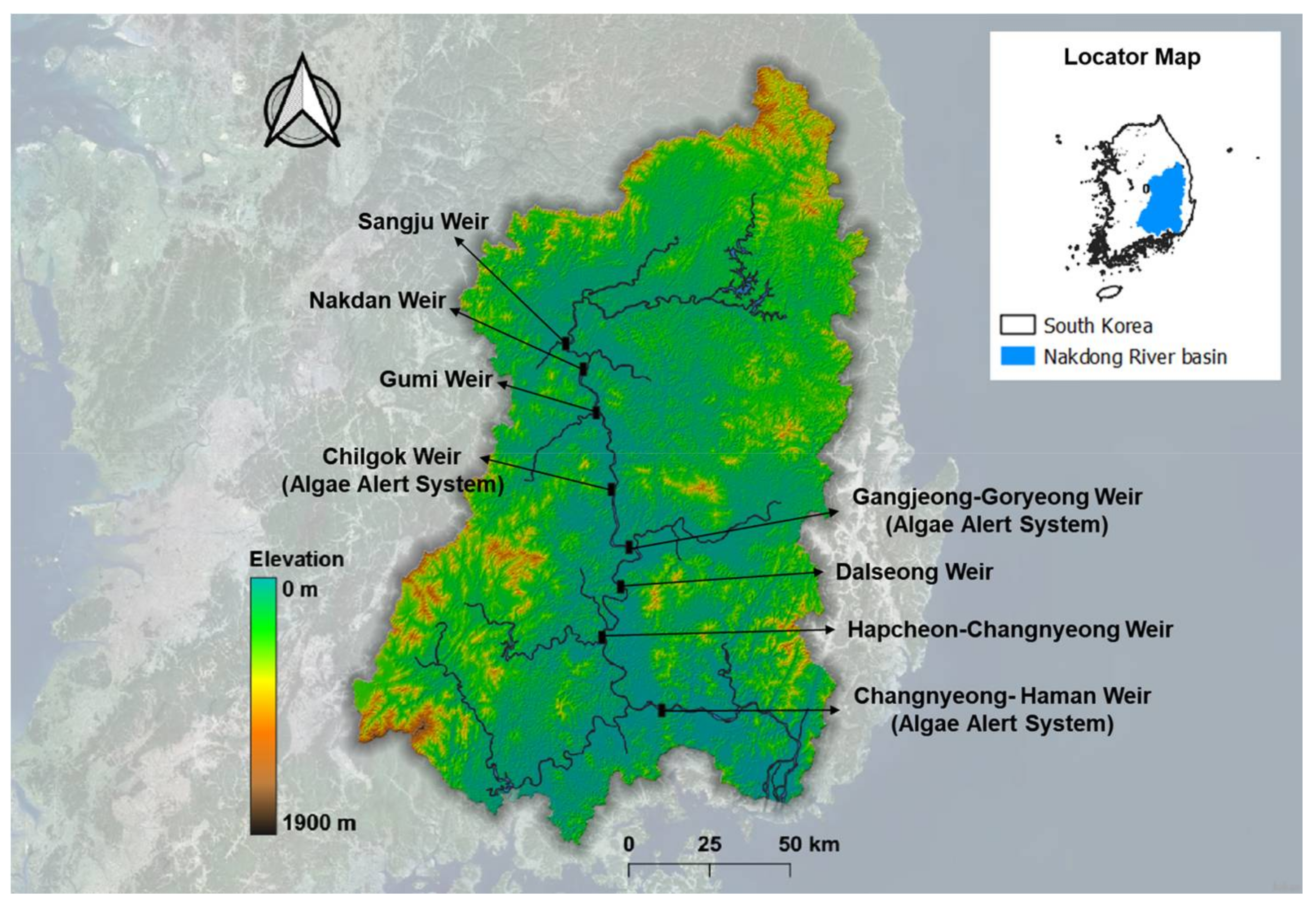
2.1. Study Area

Since 2012, 16 weirs have been operated on the four major rivers of South Korea; Hang River, Nakdong River, Geum River, and Yeongsan River [10]. The longest, Nakdong River [21] with a length of about 510 km, has been exposed to water quality problems due to adjacent industrial and agricultural districts [2]. In the Nakdong river basin, there are eight weirs [2,21], whose locations are shown in Figure 1.

Among the eight weirs, we selected Chilgok weir, completed in June 2012, as the target location of this study for two reasons. The first reason is the availability of the datasets related to the cyanobacterial blooms of Chilgok weir. The Algae Alert System in South Korea [2], based on cyanobacterial cell density as shown in

Table 1. Criteria for algae alert in South Korea.

Stage	Cyanobacterial Cell Density (cells mL−1)
Caution	≥1000
Warning	≥10,000
Outbreak	≥1,000,000

[2,9,23], has been operated by the National Institute of Environmental Research (NIER) to ensure the safety of drinking water [23]. One of the observation stations is at the upstream point about 500 m away from Chilgok weir [2]. The second is the location of the observation station. The station of Chilgok weir is located in the most upstream point among three stations involved in the Algae Alert System on the mainstream of Nakdong River. It enables us to consider as few factors as possible influencing the cyanobacterial blooms. In general, there are more factors in the downstream points affecting the occurrence of cyanobacterial blooms, such as the inflow of pollutants from tributaries or sewage treatment plants [2,21].

2.2. Dataset

2.2.1. Data Availability

For Chilgok weir point, we acquired datasets including water quality factors, climatic conditions, and hydrological factors known as the causes (or influencing factors) of the cyanobacterial blooms. Cyanobacteria-related water quality data, meteorological data, and hydrological data are open to the public by NIER, Korea Meteorological Administration (KMA), and Korea Water Resources Corporation (K-water), respectively [2,9,14,15,21,23,29,32].

Table 2. List of features.

Category	Feature	Description	Unit	Frequency	Source
Water quality data	Cyano	Cyanobacterial cell density	cells mL−1	Weekly	NIER
	WT	Water temperature	°C
	pH	Hydrogen ion concentration	-
	DO	Dissolved oxygen	mg L−1
	Chl-a	Chlorophyll a	mg m−3
	BOD	Biochemical oxygen demand	mg L−1
	COD	Chemical oxygen demand	mg L−1
	SS	Suspended solids	mg L−1
	TN	Total nitrogen	mg L−1
	TP	Total phosphorus	mg L−1
	N/P	TN/TP ratio	-
	TOC	Total organic carbon	mg L−1
	EC	Electrical conductivity	μS cm−1
	TotalColiform	Total coliforms	100 mL−1
	TDN	Total dissolved nitrogen	mg L−1
	NH3-N	Ammonium nitrogen	mg L−1
	NO3-N	Nitrate nitrogen	mg L−1
	TDP	Total dissolved phosphorus	mg L−1
	PO4-P	Phosphate phosphorus	mg L−1
	FecalColiform	Fecal coliforms	-
Meteorological data	AT	Average air temperature	°C	Daily	KMA
	LT	Lowest air temperature	°C
	HT	Highest air temperature	°C
	MaxSolarRad	Maximum amount of solar radiation for one hour	MJ m−2
	DaySolarRad	Total amount of solar radiation	MJ m−2
Hydrological data	WeirLevel	Water level of weir	EL.m	Daily	K-water
	StorageVolume	Storage volume of weir	million m3
	Rainfall	Rainfall in weir catchment area	mm
	Inflow	Weir inflow	m3 s−1
	Outflow	Weir outflow	m3 s−1

shows the feature, the frequency, and the source of each dataset. Regarding the cyanobacteria-related water quality, the harmful cyanobacteria include four genera: Microcystis, Anabaena, Aphanizomenon, and Oscillatoria spp. [2,9,23].

2.2.2. Data Preprocessing

Across a range of regions, there were previous studies in which the forecast horizons were set from real-time to as long as one month or more depending on the objective of developing the models and the frequency of the used datasets [16]. In this study, we used a week as the forecast horizon because the frequency of the cyanobacteria-related water quality dataset is on a weekly basis as shown in Table 2. The raw dataset consisted of 378 instances with the cyanobacterial cell density after a week (Cyano(t+1)) as a target variable and 30 input features including the current cell density (Cyano(t)) as shown in

Table 3. Nine-year mean, minimum, median, and maximum values for each feature in the raw dataset (378 instances).

Category	Feature	Mean	Minimum	Median	Maximum
Input features	Cyano(t)	2976	0	165	112,735
	WT	16.8	0.7	17.5	33.6
	pH	8.1	6.5	8.1	9.6
	DO	10.4	1.6	10.1	16.4
	Chl-a	20.1	2.3	15.45	87.2
	BOD	1.9	0.4	1.8	5.0
	COD	5.9	3.5	5.8	10.5
	SS	7.6	1.5	6.3	44.9
	TN	2.674	1.089	2.686	4.396
	TP	0.043	0.011	0.034	0.198
	N/P	81.5	12.7	76.6	255.5
	TOC	4.1	2.6	4.0	7.9
	EC	288	124	286	596
	TotalColiform	8219	2	264	340,000
	TDN	2.513	1.078	2.532	4.125
	NH3-N	0.113	0.003	0.091	0.790
	NO3-N	1.971	0.530	1.996	3.330
	TDP	0.024	0.003	0.018	0.125
	PO4-P	0.011	0.000	0.004	0.105
	FecalColiform	428	0	12	21,750
	AT	15.5	−4.8	15.8	32.5
	LT	10.8	−8.9	10.8	27.6
	HT	21.0	−1.0	21.9	38.0
	MaxSolarRad	2.39	0.19	2.54	3.74
	DaySolarRad	15.56	0.69	15.465	31.02
	WeirLevel	25.52	25.02	25.56	25.86
	StorageVolume	75.321	68.181	75.930	79.005
	Rainfall	2.290	0.000	0.023	57.263
	Inflow	112.867	3.604	67.733	1147.669
	Outflow	113.379	8.098	69.004	1140.136
Target variable (Output feature)	Cyano(t+1)	2903	0	165	112,735

. The period for the used data was from August 2012 to December 2020.

The machine learning models applying classification algorithms require a nominal or an ordinal data type for target variables [30]. In order to compare the performance of each model depending on the number of classes, we made three groups by classifying the target variable (Cyano(t+1)) based on the Algae Alert System, as presented in Table 1. For the first group, the dataset was classified into four classes (Normal, Caution, Warning, and Outbreak), which was the same as the Algae Alert System, and it was named Group1. It had an imbalanced dataset as it comprised 269 Normals, 83 Cautions, 26 Warnings, and zero Outbreaks. We made the other two groups (Group2 and Group3) by dividing the dataset into two classes (e.g., [9]) (Normal/Occurrence) for Group2 and three classes (e.g., [22,23]) (None/Normal/Occurrence) for Group3. As a result, Group1, Group2, and Group3 consisted of four, two, and three classes, respectively. We used these three groups to ensure which classification of the cyanobacterial cell density provided us with a better model with reference to performance.

Table 4. Classification framework for each group.

Group1			Group2			Group3
Class	Cyano(t+1)	Number	Class	Cyano(t+1)	Number	Class	Cyano(t+1)	Number
Normal	<1000	269	Normal	<1000	269	None	0	136
Caution	≥1000	83	Occurrence	≥1000	109	Normal	<1000	133
Warning	≥10,000	26	-			Occurrence	≥1000	109
Outbreak	≥1,000,000	0				-

shows how each group was specified in terms of cyanobacterial cell density.

In addition, the logarithmic transformation of base 10 was applied to Cyano(t) to convert the skewed distribution of the raw dataset into normal distribution as much as possible [31]. Consequently, it was named as logCyano. Here, when Cyano(t) was zero, logCyano was also given zero. Furthermore, we applied standardization to 30 input features according to Equation (1). It is one of the feature scaling methods, which is an important preprocessing task in machine learning modeling [30,33].

$$x^{\prime }=\frac{x-\mu }{\sigma }$$

(1)

where $x$′ is a standardized value, $x$ is an observation data for a specific feature from the raw dataset, $\mu$ is the mean of the whole observation data for the feature, and $\sigma$ is its standard deviation.

Table 5. Input features (including the mean, minimum, median, and maximum values for each feature) after preprocessing the dataset using logarithmic transformation and standardization, together with the classified target variable.

Category	Feature	Mean	Minimum	Median	Maximum
Input features	logCyano	0.000	−1.200	0.224	2.046
	WT		−1.974	0.085	2.071
	pH		−3.340	0.032	3.193
	DO		−3.115	−0.077	2.144
	Chl-a		−1.194	−0.310	4.514
	BOD		−2.066	−0.148	4.237
	COD		−2.316	−0.100	4.430
	SS		−1.240	−0.280	7.533
	TN		−2.451	0.018	2.661
	TP		−1.219	−0.329	6.019
	N/P		−1.602	−0.114	4.048
	TOC		−1.784	−0.133	4.468
	EC		−2.312	−0.041	4.324
	TotalColiform		−0.308	−0.299	12.455
	TDN		−2.357	0.031	2.646
	NH3-N		−1.213	−0.243	7.458
	NO3-N		−2.425	0.042	2.288
	TDP		−1.045	−0.307	4.957
	PO4-P		−0.570	−0.355	5.068
	FecalColiform		−0.252	−0.245	12.520
	AT		−2.286	0.024	1.907
	LT		−2.182	0.000	1.861
	HT		−2.372	0.088	1.826
	MaxSolarRad		−2.567	0.171	1.569
	DaySolarRad		−2.103	−0.014	2.186
	WeirLevel		−3.042	0.219	2.030
	StorageVolume		−3.250	0.277	1.677
	Rainfall		−0.349	−0.346	8.381
	Inflow		−0.751	−0.310	7.111
	Outflow		−0.723	−0.305	7.054
Target variable	Each class of three groups (Group1, Group2, and Group3) based on Cyano(t+1)

shows the values of the input features after preprocessing using the logarithmic transformation and the standardization of input features, together with the classified target variable.

2.3. Feature Selection

2.3.1. Analysis of Variance (ANOVA)

To build robust learning models, we need feature selection, leading to the elimination of redundant and irrelevant features [24]. This helps prevent overfitting, enhance model performance, and increase the running speed of a model [24]. The filter approach, one of the feature selection methods [24], uses techniques such as ANOVA, which is widely used in statistical studies. One-way ANOVA determines whether differences between two or more classes are statistically significant through a comparison of variances between classes [34]. Through one-way ANOVA, we can judge that the difference is significant when the F value is large enough and the p-value is less than 0.05 [34,35]. In this study, features with valid F and p values (F value > 50, p-value < 0.05) by one-way ANOVA were selected to develop the machine learning models for three groups formed by using the categorical variables [36]. This is because significant F and p values mean the features have a high correlation with the categorical target variable.

2.3.2. Multi-Collinearity

Multi-collinearity arises when inter-correlation between input features is strong [27,28]. It can be a problem in statistical analysis such as regression as it distorts the prediction results of the model [27,28]. For classification-based machine learning, the multi-collinearity problem can be addressed as part of feature selection (e.g., [27,37,38,39]). In this study, features with weak inter-correlation are candidates to be selected. To be specific, the features with high inter-correlation are removed after correlation analysis using all the features selected through one-way ANOVA. As a result, we could achieve the purpose of feature selection, such as warding off the overfitting of the model, by having only the minimum number of features [40].

2.4. Machine Learning

2.4.1. Classification Algorithms

For this study, we applied four classification-based machine learning algorithms, k-NN, DT, LR, and SVM, which are widely used [41]. The k-NN is a distance-based classification algorithm that finds the ‘k’ neighbors, which are closest to the data to be classified. The target data are allocated the same label as the closest neighbors [22]. The DT is a technique of classifying data based on the impurity of training data, such as the Gini index [29] and the entropy [42]. The LR is a classification method that uses logit functions to predict the probability that data fall into a category between zero and one [43]. Multinomial logistic regression, an extended form of LR, allows multiple classes to be applied [43]. The SVM is a machine learning algorithm that determines the optimal hyperplane to maximize the distance between the categories. The class of new data is determined by the hyperplane [22]. These four machine learning techniques can be implemented using scikit-learn, one of Python’s machine learning libraries [30].

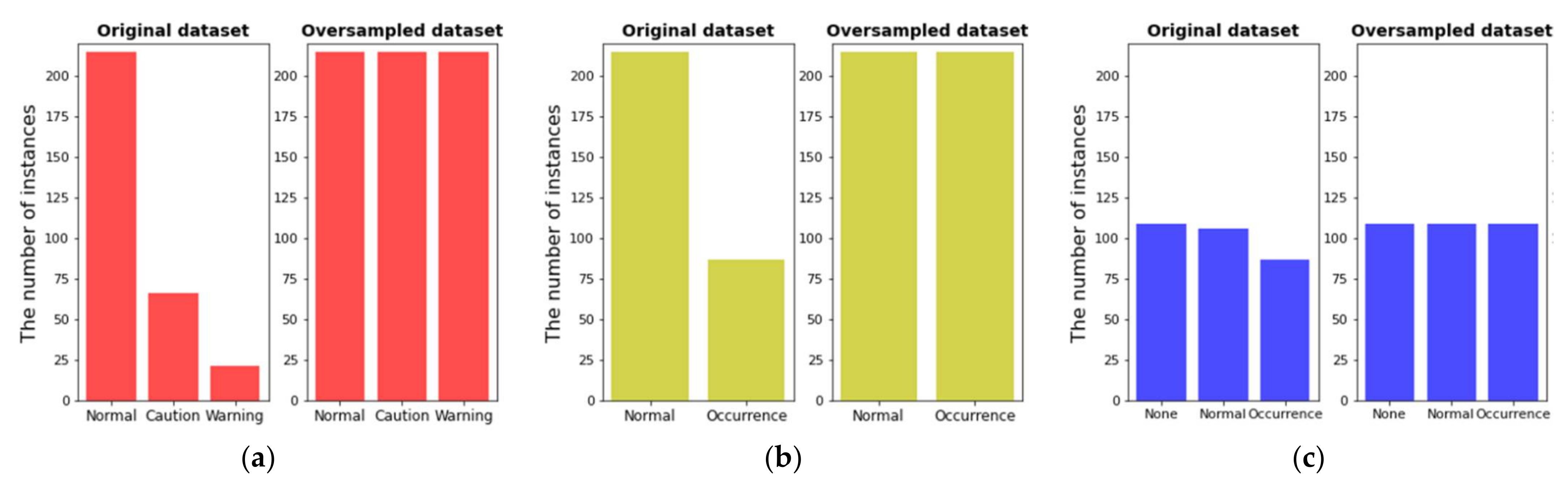
2.4.2. Oversampling Using SMOTE (Synthetic Minority Oversampling Technique)

As shown in Table 4 regarding the classification frameworks of three groups (Group1, Group2, and Group3), the dataset to be used in this study had an imbalance by class in all three groups. While the application of machine learning using such an imbalanced dataset gives rise to overfitting by increasing excessively prediction accuracy for the majority class [44], it may make an inaccurate prediction for the minority class [29]. To overcome the problem of an imbalanced dataset, oversampling can be applied, leading to improved prediction accuracy for minority classes. It is a process of producing new data of minority classes equal to the number of data belonging to a majority class [31].

One of the widely used oversampling techniques is SMOTE [45]. It is a method of synthesizing the interpolated points on a line connecting between adjacent groups of a minority class in a training set and labeling them as new samples of the minority class [29,31,45]. Shin et al. [29] and Choi et al. [31] suggested that the cyanobacterial-related models to which SMOTE was applied outperformed those without oversampling. In this study, SMOTE was employed by using a Python library, imblearn [30].

2.4.3. Training, Cross-Validation, and Test

The dataset should be split into a training set for learning and a test set for verification of the model [30]. In this study, the split ratio between the training set and the test set was 80%:20%. Additionally, four-fold cross-validation was performed on the training set to prevent the overfitting of the model [46]. At the same time, the optimal parameters for each classification algorithm were found through grid search that could improve the model performance [30,46]. Finally, the models built through four-fold cross-validation were evaluated using the test set. The parameters which were optimized in this study are shown in

Table 6. Parameters to be optimized in this study for four algorithms.

Algorithm	Parameter	Description
k-NN	n_neighbors	Number of neighbors
DT	max_depth	Maximum depth of the tree
LR	C	Regularization parameter
SVM	C	Regularization parameter
	kernel	The kernel type to be used in the algorithm such as ‘linear’, ‘poly’, ‘rbf’, ‘sigmoid’, etc.

[30].

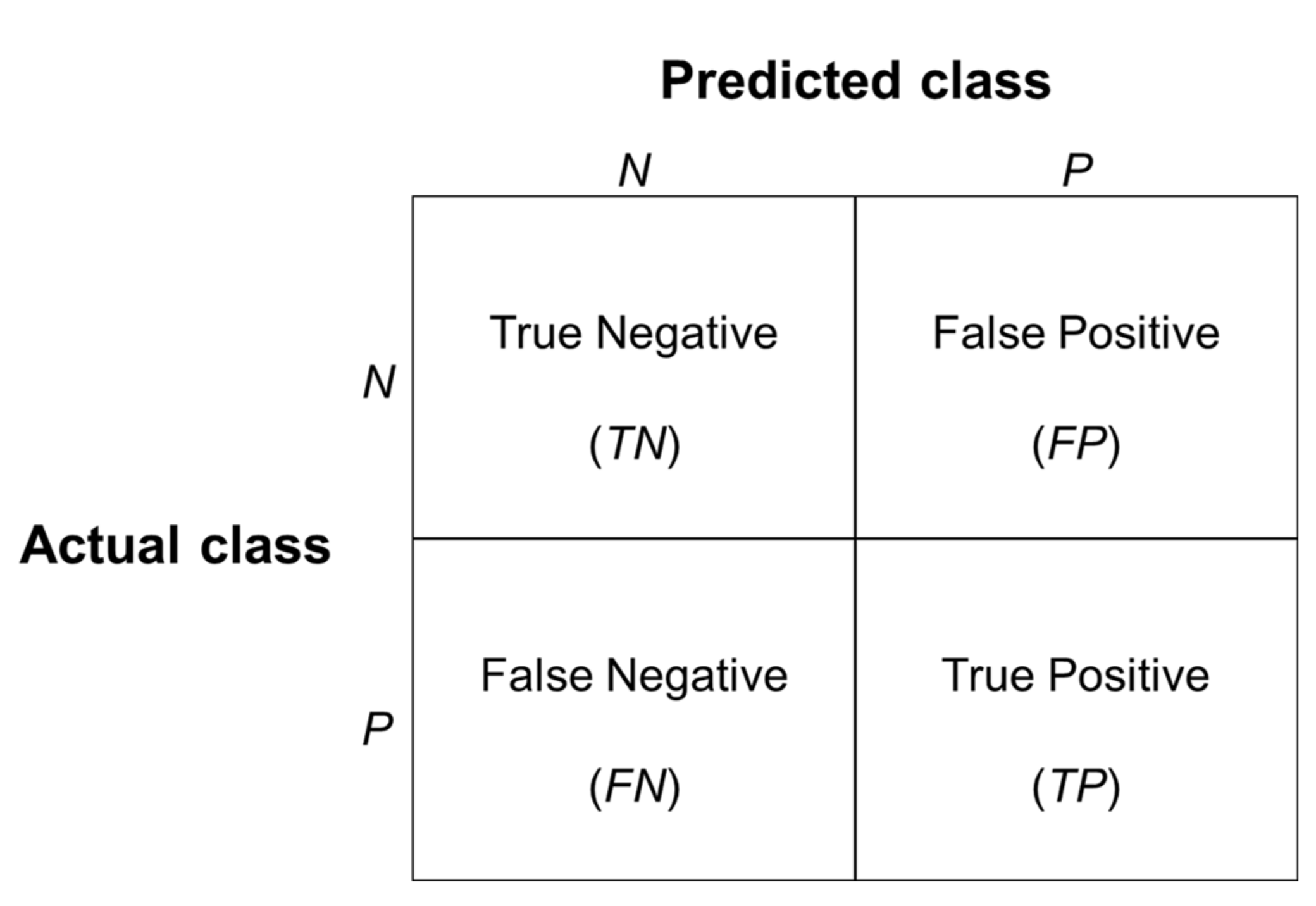
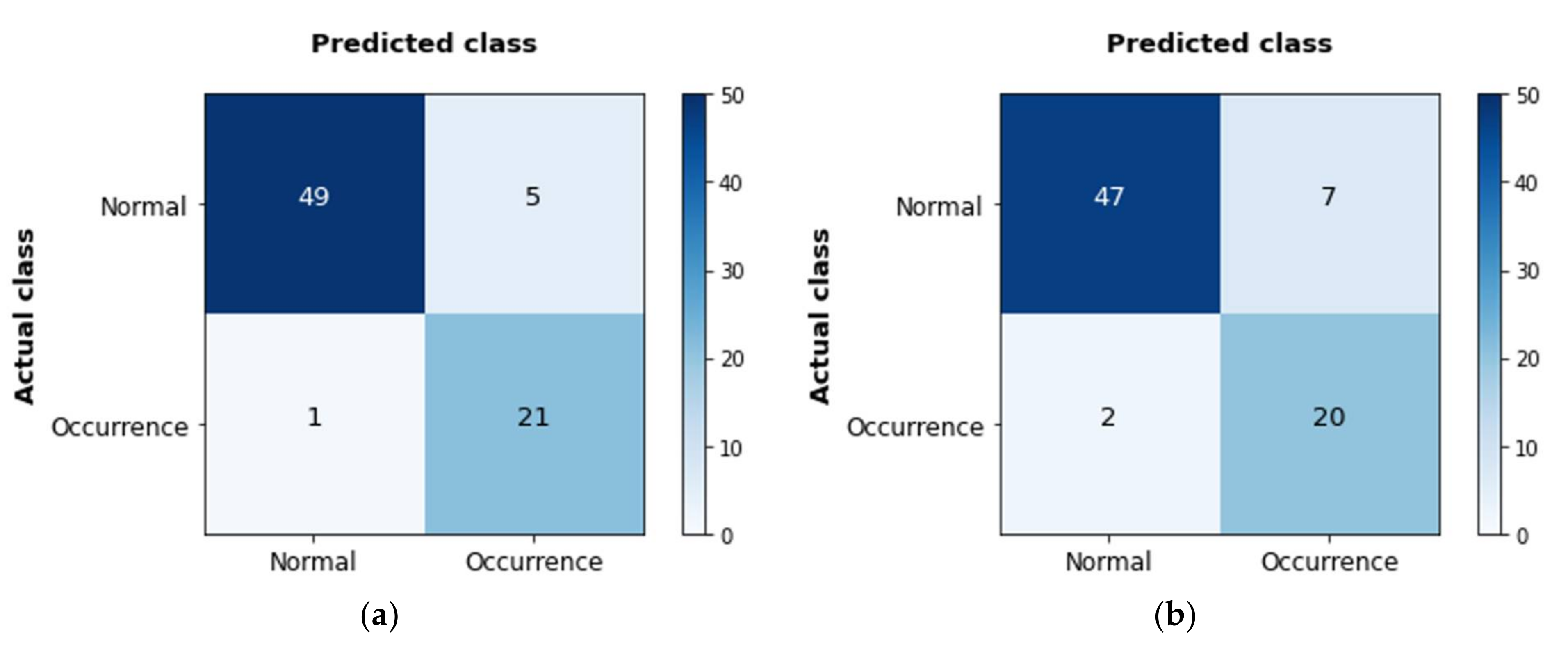
2.4.4. Model Evaluation

The metrics that evaluate the performance of the classification model include Accuracy (ACC), Precision (PRE), Recall (REC), and F1-score (F1) [30,44,47]. As shown in Figure 2 [30], we can describe each metric through a confusion matrix schematizing binary classification using True Positive (TP), True Negative (TN), False Positive (FP), and False Negative (FN). Accuracy is obtained by dividing the sum of correct predictions (TP + TN) by the total number of data. Precision represents the ratio of TP to the total number of samples predicted to be positive (TP + FP). Recall indicates the ratio of TP to the total number of samples belonging to the actual positive class (TP + FN). F1-score is expressed as a harmonic mean of Precision and Recall [47]. Precision, Recall, and F1-score are known as the more reliable metrics for an imbalanced dataset than Accuracy [47]. We, however, used Accuracy as a performance evaluation metric in this study. The reasons are that we developed the models using a balanced dataset through SMOTE and we needed to see their accuracy for both Negatives and Positives of the predicted classes. The four metrics are formulated as follows [30,44,47].

$$ACC=\frac{TP+TN}{TP+TN+FP+FN}$$

(2)

$$PRE=\frac{TP}{TP+FP}$$

(3)

$$REC=\frac{TP}{TP+FN}$$

(4)

$$F1=2 \frac{PRE\times REC}{PRE+REC}$$

(5)

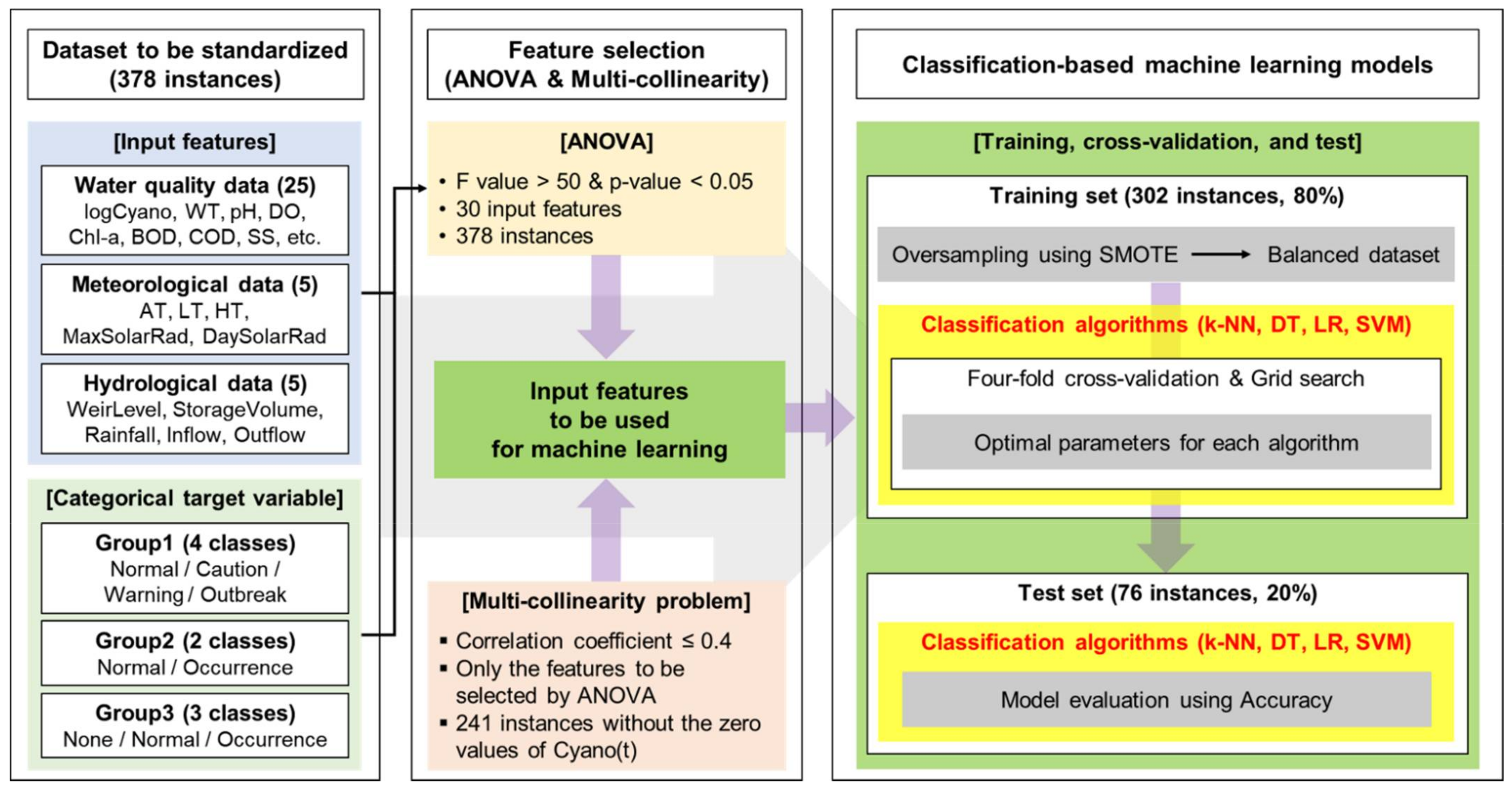
2.5. Summary of the Modeling Procedure

We summarized the modeling procedure as follows with Figure 3, based on the above subsections.

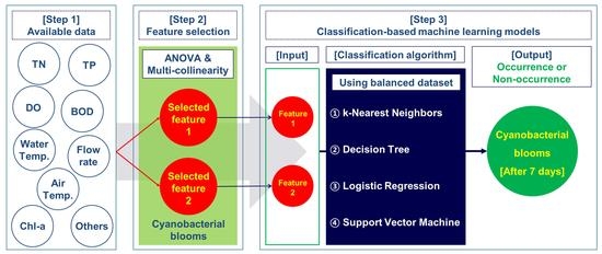
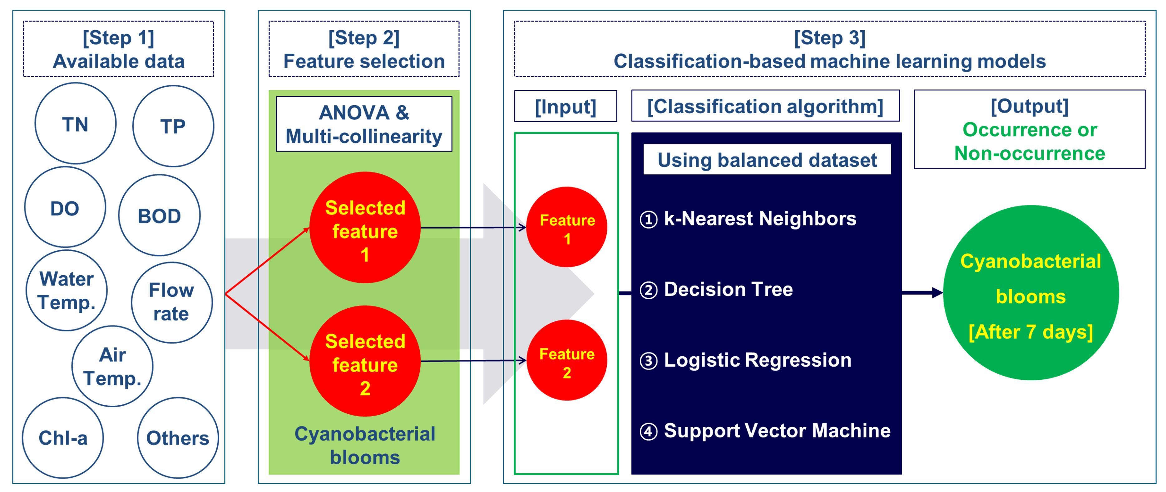
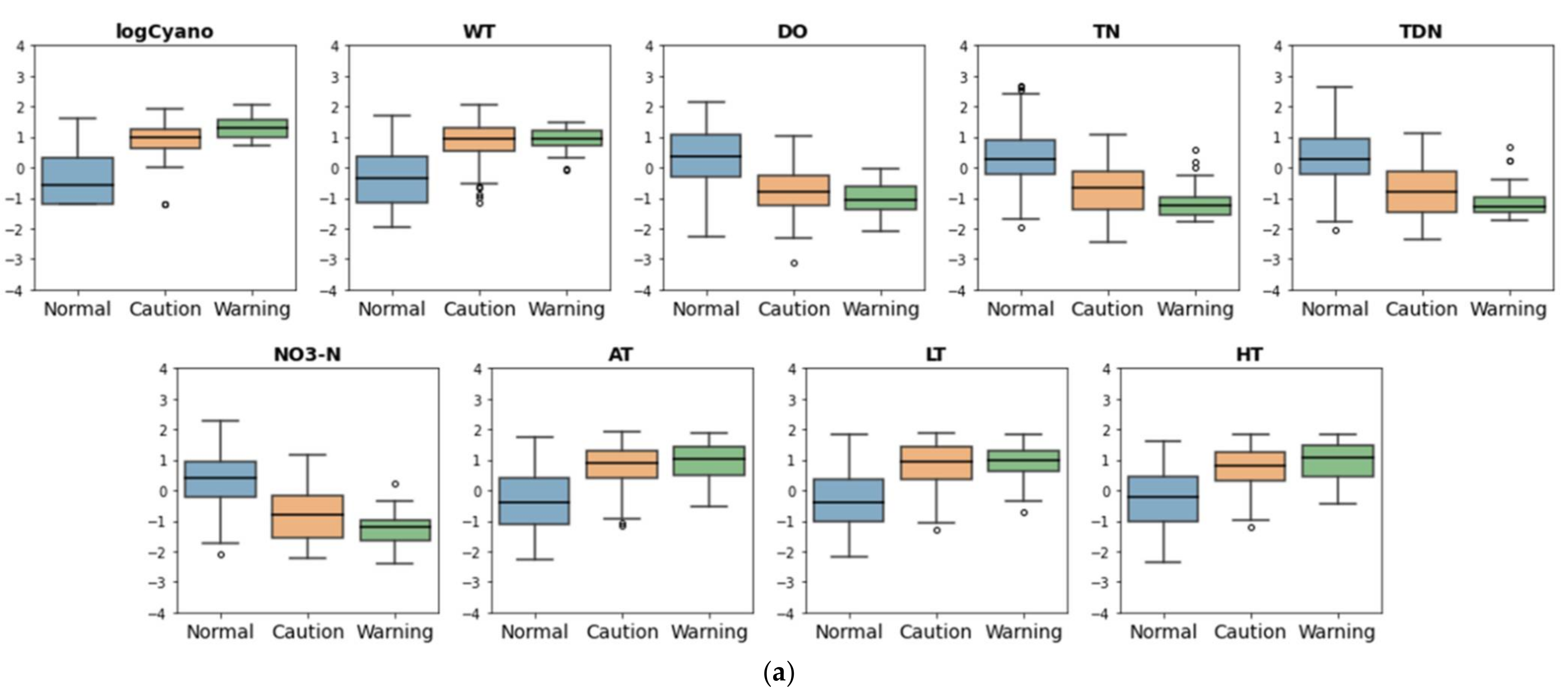
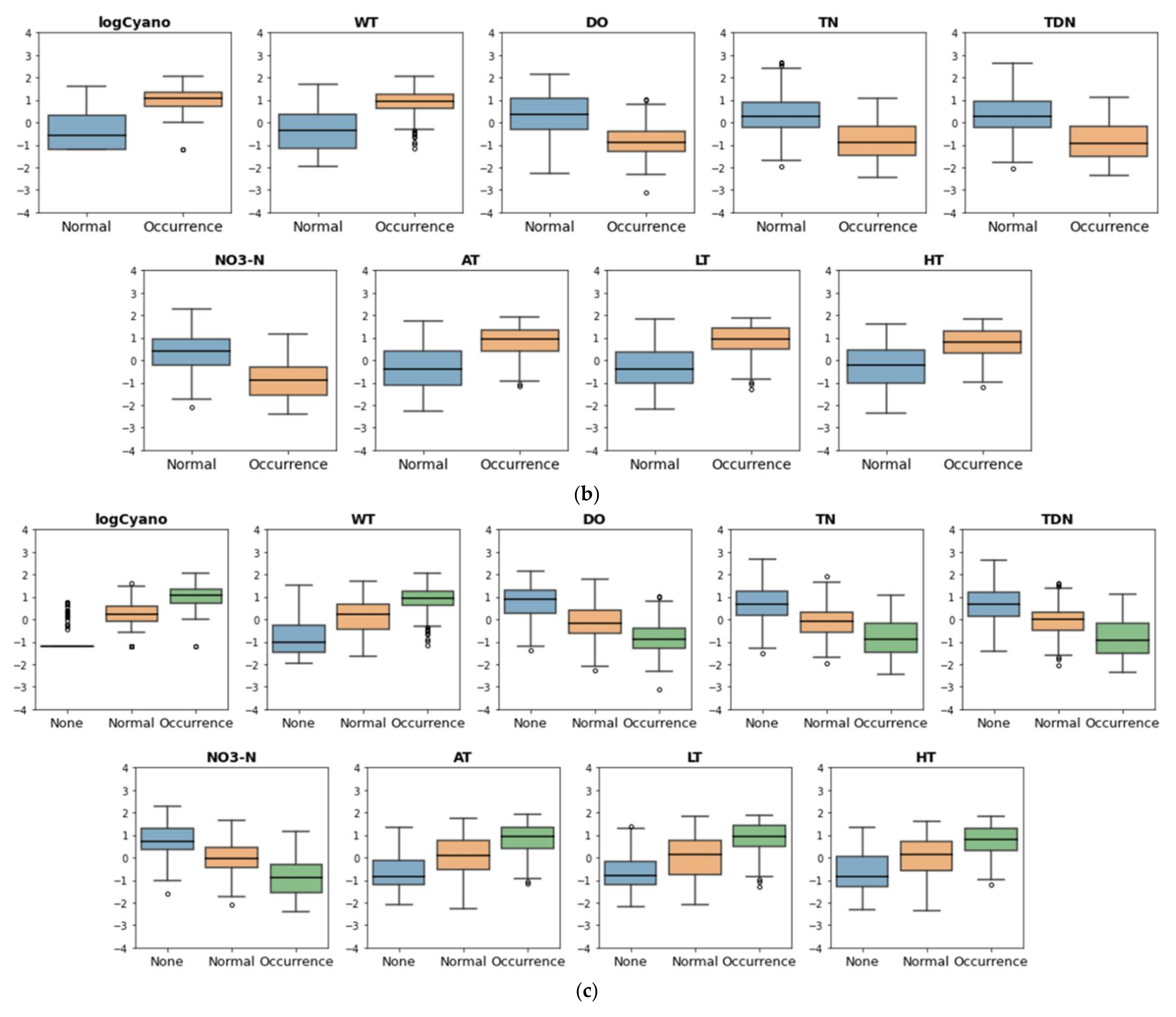
• One-way ANOVA was carried out using 30 features including logCyano of a standardized dataset with 378 instances for three groups (Group1, Group2, and Group3). For the purpose of selecting the features having a strong correlation with the target variable, F values of more than 50 and p-values of less than 0.05 [34,35] were applied. Here, the target variable was a class based on Cyano(t+1) for each group; Normal/Caution/Warning/Outbreak for Group1 (which was actually divided into three classes because the number of Outbreak elements was zero), Normal/Occurrence for Group2, and None/Normal/Occurrence for Group3.
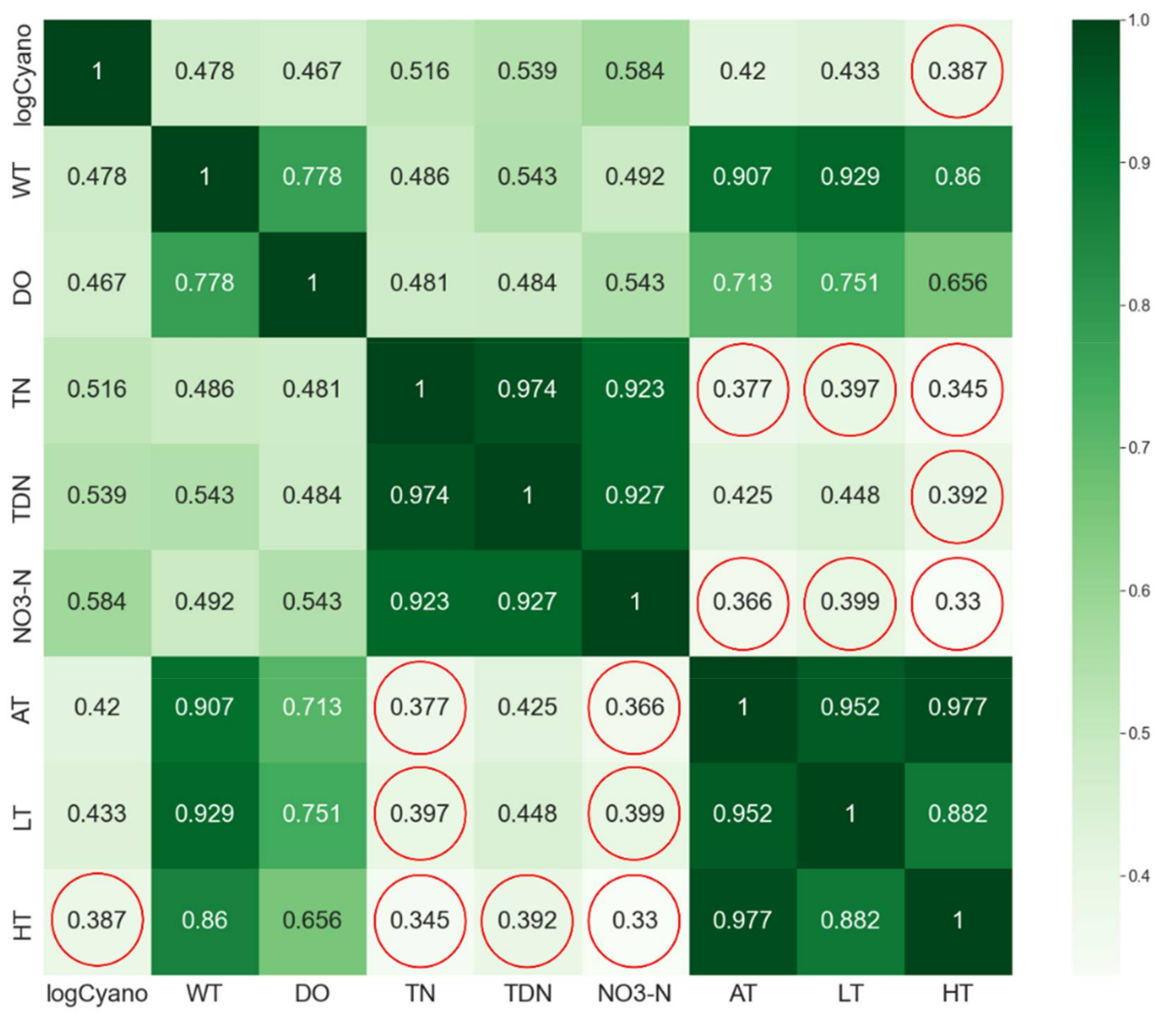
• To address the multi-collinearity problem, the correlation analysis was performed among the features selected in the first step. As the final process for the feature selection, the paired features with low inter-correlation coefficients (0.4 or less [48,49]) were selected. Here, Pearson’s correlation analysis was performed with only 241 instances by excluding the zero values of Cyano(t) in 378 instances, as the zero values were able to distort the analysis result.
• The dataset consisting of the input features selected in the second step and the target variable was split into a training set and a test set by 80% and 20%. Therefore, 302 and 76 out of 378 instances were used as the training set and the test set, respectively. After that, oversampling for the training set was performed [31] by applying SMOTE. As a result of the oversampling, the number of instances by class became the same.
• Using the balanced datasets of three groups acquired in the third step, four classification-based machine learning algorithms including k-NN, DT, LR, and SVM, were applied. The models with optimal parameters for each machine learning method were constructed through four-fold cross-validation and grid search using the training set.
• The optimal combination of input features and machine learning algorithms for predicting the categorical target variable was presented by evaluating the performance (Accuracy) from the test set using the models developed in the fourth step.

3. Results

3.1. Determination of the Modeling Cases

We could determine the modeling cases based on the result of feature selection. Through one-way ANOVA, as shown in

Table 7. F and p values of 30 features. (The nine features with the bold font have significant F and p values).

Feature	Group1		Group2		Group3
	F Value	p-Value	F Value	p-Value	F Value	p-Value
logCyano	132.367	<0.001	256.089	<0.001	270.917	<0.001
WT	71.613	<0.001	143.214	<0.001	142.227	<0.001
pH	0.545	0.580	0.313	0.576	6.180	0.002
DO	74.182	<0.001	145.698	<0.001	131.458	<0.001
Chl-a	7.137	0.001	14.118	<0.001	7.637	0.001
BOD	1.463	0.233	2.917	0.088	5.022	0.007
COD	2.599	0.076	5.186	0.023	18.898	<0.001
SS	5.244	0.006	3.924	0.048	4.928	0.008
TN	63.964	<0.001	123.352	<0.001	108.115	<0.001
TP	4.222	0.015	0.951	0.330	6.432	0.002
N/P	19.436	<0.001	38.336	<0.001	40.293	<0.001
TOC	1.499	0.225	1.456	0.228	18.843	<0.001
EC	6.176	0.002	0.170	0.680	8.701	<0.001
TotalColiform	4.703	0.010	6.984	0.009	7.137	0.001
TDN	66.039	<0.001	128.394	<0.001	103.655	<0.001
NH3-N	5.961	0.003	11.281	0.001	6.176	0.002
NO3-N	85.820	<0.001	163.285	<0.001	126.452	<0.001
TDP	3.874	0.022	2.428	0.120	12.020	<0.001
PO4-P	2.922	0.055	0.594	0.441	8.241	<0.001
FecalColiform	1.754	0.175	3.176	0.076	5.414	0.005
AT	63.407	<0.001	126.277	<0.001	98.519	<0.001
LT	66.861	<0.001	133.669	<0.001	103.961	<0.001
HT	53.737	<0.001	106.578	<0.001	83.166	<0.001
MaxSolarRad	5.712	0.004	9.368	0.002	6.774	0.001
DaySolarRad	4.996	0.007	7.154	0.008	5.754	0.003
WeirLevel	3.047	0.049	4.768	0.030	9.661	<0.001
StorageVolume	2.737	0.066	4.370	0.037	9.695	<0.001
Rainfall	2.256	0.106	0.370	0.543	0.327	0.721
Inflow	3.843	0.022	0.244	0.622	6.501	0.002
Outflow	3.649	0.027	0.148	0.701	6.543	0.002

, nine features such as logCyano, WT, DO, TN, TDN, NO₃-N, AT, LT, and HT had significant F and p values (F value > 50, p-value < 0.05 [34,35]) for the categorical target variable in all three groups. Figure 4 shows the box plots having the data distribution for each group for the selected nine features, which helps intuitively notice the differences between classes. As shown in Figure 4, the distinctions between classes in Group2 and Group3 are clear for the nine features, as in the results of Table 7. On the other hand, in Group1, the distinction between Normal and Caution is clear, but it is somewhat unclear between Caution and Warning. Nonetheless, we used Group1 to compare with the modeling results for the other two groups. This is because we applied the same classification as the Algae Alert System in Table 1 to Group1 and the F and p values for its three classes were significant as shown in Table 7.

Although those nine features were highly correlated with the target variable, two features among them had a multi-collinearity problem. This could be solved by eventually selecting the features with low inter-correlation coefficients (0.4 or less [48,49]). As shown in Figure 5, we could recognize that WT and DO should be eliminated because they were highly correlated with the other features. Accordingly, we were able to make eight modeling cases, which consisted of two features as shown in

Table 8. Modeling cases with a combination of input features.

Modeling Case	Input Features
Case1	logCyano, HT
Case2	TN, AT
Case3	TN, LT
Case4	TN, HT
Case5	TDN, HT
Case6	NO3-N, AT
Case7	NO3-N, LT
Case8	NO3-N, HT

.

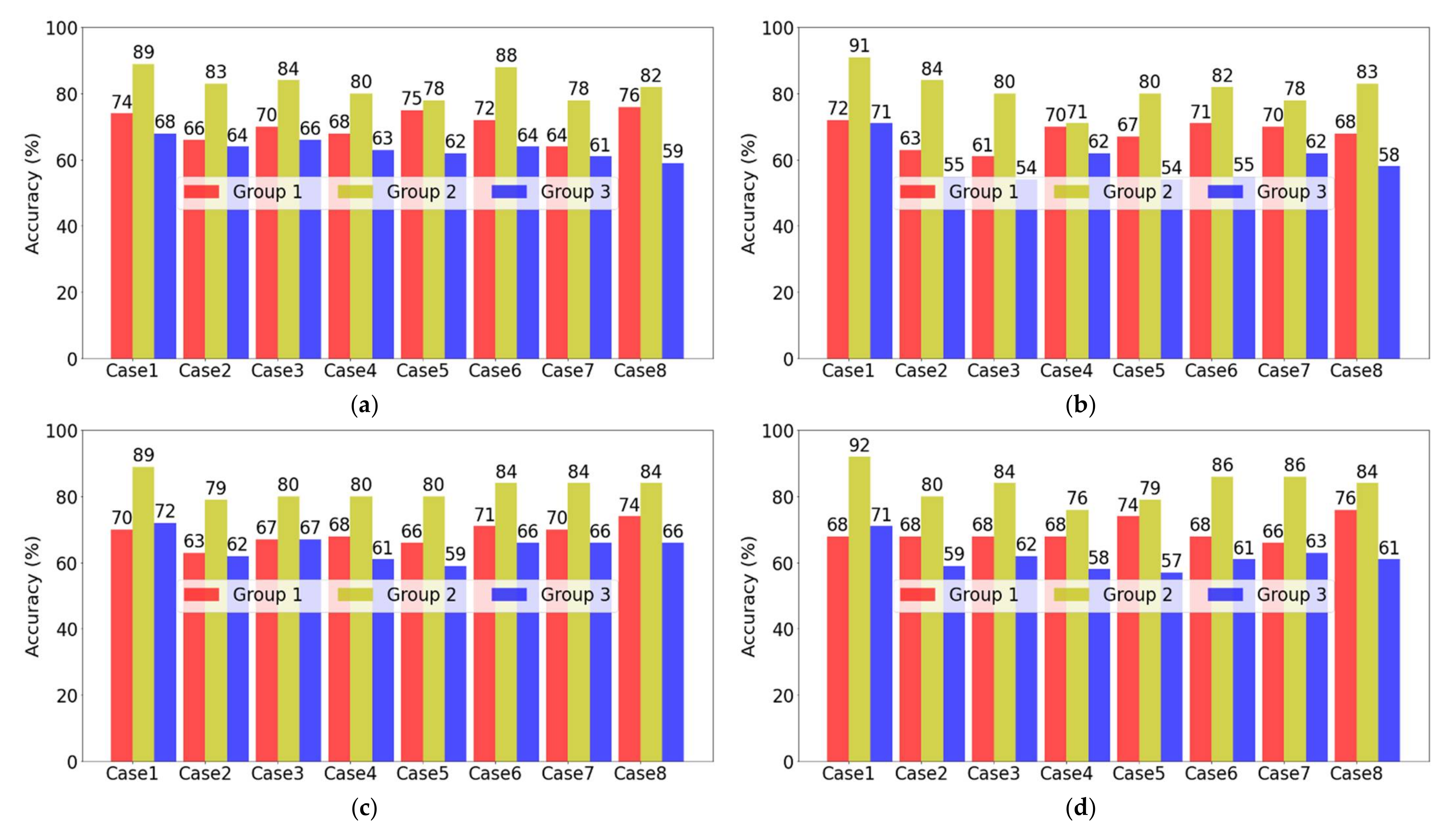
3.2. Accuracy of the Models

For eight modeling cases, the machine learning models were developed using four classification algorithms: k-NN, DT, LR, and SVM. Prior to applying those algorithms, oversampling for the training sets was implemented for the eight cases by a group as shown in Figure 6. As a result, a total of 96 models were built with the balanced datasets of the three groups for the eight cases using four machine learning techniques.

Table 9. Optimized parameters of four classification algorithms.

Algorithm (Parameter)	Group	Case1	Case2	Case3	Case4	Case5	Case6	Case7	Case8
k-NN (n_neighbors)	Group1	3	11	12	6	6	7	3	5
	Group2	3	16	13	13	9	5	5	3
	Group3	19	16	19	17	16	10	14	14
DT (max_depth)	Group1	15	11	10	9	15	9	12	14
	Group2	1	3	4	14	14	10	8	6
	Group3	3	4	3	3	3	4	3	2
LR (C)	Group1	0.01	1	0.001	0.1	1	0.01	0.01	0.001
	Group2	1	1	100	1	0.1	10	1	1
	Group3	1	10	100	100	0.1	10	1	1
SVM (C/kernel)	Group1	1000/rbf	1000/rbf	1000/rbf	1000/rbf	1000/rbf	1000/rbf	1000/rbf	1000/rbf
	Group2	10/linear	1/rbf	1/rbf	0.1/rbf	1/rbf	1/rbf	100/rbf	100/rbf
	Group3	10/rbf	100/rbf	10/linear	1/linear	0.1/rbf	0.1/rbf	1/linear	0.1/rbf

shows the parameters optimized by four-fold cross-validation and grid search of each model using the training sets. One thing we need to note in this table is that the parameter max_depth of the Case1 model using Group2 and the DT algorithm (DT-Group2-Case2) is one. It means that only one of the two input features was used to build the model, so we have to be careful when using this model.

We could verify which model was more accurate using the test sets as shown in Figure 7. The combination of SVM-Group2-Case1 using logCyano and HT as input features provided us with the most accurate model for predicting the cyanobacterial blooms of Chilgok weir, which ensured the highest accuracy of 92% among the 96 models. On the other hand, the model accuracy of DT-Group3-Case3 and DT-Group3-Case5 was the lowest at 54%.

Of the 96 models, 25 models with an accuracy of 80% or more came from Group2, but all 10 models with less than 60% were from Group3. The accuracy of all the models using Group2 with two classes was higher than the other groups with three classes. Moreover, when evaluating performance based on the used features, we could confirm the highest accuracy of the models using logCyano as a feature. Among the models without using logCyano, the ones with NO₃-N ensured the highest accuracy except the DT algorithm. To be specific, we obtained the highest accuracy of 88% in the models of k-NN-Group2-Case6 except for four models using logCyano. Figure 8 shows the confusion matrices for the two models, each with the highest accuracy when using logCyano (SVM-Group2-Case1) and when not using it (kNN-Group2-Case6). We could see that both models provided results that were not biased overall towards non-occurrence or occurrence.

3.3. Summary of the Modeling Results

The results of the modeling study can be summarized as follows:

• We had nine input features including logCyano, WT, DO, TN, TDN, NO₃-N, AT, LT, and HT from 30 input features by applying one-way ANOVA.
• Seven input features except for WT and DO were available finally for model construction due to the multi-collinearity problem.
• By using only two input features, we could build a model with a prediction accuracy of more than 80%.
• The models using Group2 with two classes surpassed the other models using Group1 and Group3 that were divided into three classes in terms of model performance.
• The optimal combination, developing the most accurate model was SVM-Group2-Case1, whose accuracy was the highest at 92%.
• All the models with the highest accuracy for each of the four machine learning algorithms (k-NN, DT, LR, and SVM) included logCyano as a feature.
• Among the models that did not use logCyano as a feature, the ones in combination with air temperature (AT, LT, or HT) and NO₃-N enabled high predictive accuracy of more than 80%.

These results will enable the concerned decision makers to understand how to build classification-based machine learning models for predicting the occurrences of cyanobacterial blooms (HABs) efficiently and effectively. They also indicate that monitoring the cyanobacterial cell density closely is very important for predicting HABs. For further prevention or minimization of HABs, actions could be considered targeting a reduction in pollutants in the water (e.g., NO₃-N), or reducing water temperature (e.g., by selective releases from upstream reservoirs, which do exist in the case study area considered). It should be noted, however, that the primary goal of this analysis is the efficient and effective prediction of HABs, while actions for their prevention may be quite diverse and case-study specific.

4. Discussion and Conclusions

We developed and evaluated the classification-based machine learning models to predict the cyanobacterial blooms after a week for Chilgok weir in South Korea. In order to build accurate models, we went through important processes such as feature selection, oversampling for the imbalanced dataset, and application of classification algorithms.

Through the feature selection, we could not retain features such as water temperature, total phosphorus, solar radiation, discharge, etc., which are theoretically known to affect the occurrence of cyanobacterial blooms [15,16]. However, it is noted that this was the result of the targeted data reduction, namely applying ANOVA and solving the multi-collinearity problem. At the same time, the more important thing is that we collected the data of 30 features based on the theories of cyanobacterial blooms. It would be possible to develop a more accurate and efficient model when we would combine an understanding of the physical or biological processes for the target variable and a rational approach to data analysis simultaneously [16,25,26].

We were able to develop the classification-based machine learning models to predict cyanobacterial blooms with more than 80% accuracy using only two features. That is to say, an efficient and effective model development methodology that could increase prediction accuracy with a few features was devised. However, it was essential to select features that were involved in the target variable statistically through feature selection methods such as one-way ANOVA. Furthermore, the problems of multi-collinearity and an imbalanced dataset needed to be addressed.

We confirmed that the accuracy of the models using two classes of Group2 was overall higher than the other groups with three classes. In other words, we needed to classify the cyanobacterial density into simple two classes rather than three classes to improve the model performance. Similar to the result of this study, most multi-class classification problems are more challenging than binary ones [50]. Although we concluded that the models using Group2 outperformed the others, we have to consider how to improve the performance of the models using Group1 or Group3, which can fit the real Algae Alert System through further research.

The models using algorithms other than SVM, which accuracy was highest at 92%, also made very slight differences by achieving an accuracy of 91% for DT or 89% for k-NN and LR. On the other hand, except for the highest accuracy, the algorithms’ performances were different for different groups (Group1, Group2, and Group3) or the input features. Hence, we need to decide which machine learning algorithm should be employed by considering the application purpose of a model and the available datasets. This consideration is necessary because it would assist in determining how to encode the target variable (as binary, or as multi-class), and which input features should be used.

In predicting the cyanobacterial blooms, we could recognize that the current cyanobacterial density (Cyano(t)) had high auto-correlation with ones after a week (Cyano(t+1)). Even if this auto-correlation was not considered, it could be seen that some models using NO₃-N or TN as input features along with air temperature were also very accurate. From these results, we could assume that nitrogen compounds were directly or indirectly involved in cyanobacterial blooms [23,51]. Therefore, further research could identify if the control of nitrogen compounds flowing into rivers or reservoirs according to the air temperature is possible to make the cyanobacterial blooms produce or fade.

With regard to decision making, the predictive models using nominal or ordinal data can be more efficient than real-valued data as the results using the former type of data are much more intuitive [9]. Nevertheless, building a model based on real-valued data, rather than on a classification basis, could support more detailed decision making. Further research would be needed on whether the feature selection process presented through this study can improve the accuracy of such a model.

One of the limitations of this study relates to the fact that we did not separate the four harmful cyanobacteria genera when applying the cyanobacterial cell density [9]. Referring to the previous studies [9,22,23,29], it was our decision to acquire a sufficient number of instances for the dataset to carry out this research. Further study will be aimed at developing models involving the cyanobacteria species by reflecting a wider spectrum of their characteristics.

References

1. Tong, Y.D.; Xu, X.W.; Qi, M.; Sun, J.J.; Zhang, Y.Y.; Zhang, W.; Wang, M.Z.; Wang, X.J.; Zhang, Y. Lake warming intensifies the seasonal pattern of internal nutrient cycling in the eutrophic lake and potential impacts on algal blooms. Water Res. 2021, 188, 116570. [Google Scholar]
2. Park, H.K.; Lee, H.J.; Heo, J.; Yun, J.H.; Kim, Y.J.; Kim, H.M.; Hong, D.G.; Lee, I.J. Deciphering the key factors determining spatio-temporal heterogeneity of cyanobacterial bloom dynamics in the Nakdong River with consecutive large weirs. Sci. Total Environ. 2021, 755, 143079. [Google Scholar] [CrossRef] [PubMed]
3. Kosten, S.; Huszar, V.L.; Bécares, E.; Costa, L.S.; van Donk, E.; Hansson, L.A.; Jeppesen, E.; Kruk, C.; Lacerot, G.; Mazzeo, N. Warmer climates boost cyanobacterial dominance in shallow lakes. Glob. Chang. Biol. 2012, 18, 118–126. [Google Scholar] [CrossRef]
4. Paerl, H.W.; Huisman, J. Climate change: A catalyst for global expansion of harmful cyanobacterial blooms. Environ. Microbiol. Rep. 2009, 1, 27–37. [Google Scholar] [CrossRef] [PubMed]
5. Paerl, H.W.; Scott, J.T. Throwing fuel on the fire: Synergistic effects of excessive nitrogen inputs and global warming on harmful algal blooms. Environ. Sci. Technol. 2010, 44, 7756–7758. [Google Scholar] [CrossRef]
6. Smith, G.J.; Daniels, V. Algal blooms of the 18th and 19th centuries. Toxicon 2018, 142, 42–44. [Google Scholar] [CrossRef] [PubMed]
7. Plaas, H.E.; Paerl, H.W. Toxic Cyanobacteria: A Growing Threat to Water and Air Quality. Environ. Sci. Technol. 2021, 55, 44–64. [Google Scholar] [CrossRef]
8. Ho, L.; Goethals, P. Research hotspots and current challenges of lakes and reservoirs: A bibliometric analysis. Scientometrics 2020, 124, 603–631. [Google Scholar] [CrossRef] [Green Version]
9. Kim, S.; Kim, S.; Mehrotra, R.; Sharma, A. Predicting cyanobacteria occurrence using climatological and environmental controls. Water Res. 2020, 175, 115639. [Google Scholar] [CrossRef]
10. Song, H.; Lynch, M.J. Restoration of Nature or Special Interests? A Political Economy Analysis of the Four Major Rivers Restoration Project in South Korea. Crit. Criminol. 2018, 26, 251–270. [Google Scholar] [CrossRef]
11. Lee, S.; Kim, J.; Choi, B.; Kim, G.; Lee, J. Harmful algal blooms and liver diseases: Focusing on the areas near the four major rivers in South Korea. J. Environ. Sci. Health C 2019, 37, 356–370. [Google Scholar] [CrossRef] [PubMed]
12. Paerl, H.W. Controlling cyanobacterial harmful blooms in freshwater ecosystems. Microb. Biotechnol. 2017, 10, 1106–1110. [Google Scholar] [CrossRef] [PubMed] [Green Version]
13. Wurtsbaugh, W.A.; Paerl, H.W.; Dodds, W.K. Nutrients, eutrophication and harmful algal blooms along the freshwater to marine continuum. Wiley Interdiscip. Rev. Water 2019, 6, e1373. [Google Scholar] [CrossRef]
14. Ahn, J.M.; Kim, J.; Park, L.J.; Jeon, J.; Jong, J.; Min, J.H.; Kang, T. Predicting Cyanobacterial Harmful Algal Blooms (CyanoHABs) in a Regulated River Using a Revised EFDC Model. Water 2021, 13, 439. [Google Scholar] [CrossRef]
15. Park, Y.; Pyo, J.; Kwon, Y.S.; Cha, Y.; Lee, H.; Kang, T.; Cho, K.H. Evaluating physico-chemical influences on cyanobacterial blooms using hyperspectral images in inland water, Korea. Water Res. 2017, 126, 319–328. [Google Scholar] [CrossRef]
16. Rousso, B.Z.; Bertone, E.; Stewart, R.; Hamilton, D.P. A systematic literature review of forecasting and predictive models for cyanobacteria blooms in freshwater lakes. Water Res. 2020, 182, 115959. [Google Scholar] [CrossRef]
17. Kim, J.; Lee, T.; Seo, D. Algal bloom prediction of the lower Han River, Korea using the EFDC hydrodynamic and water quality model. Ecol. Model. 2017, 366, 27–36. [Google Scholar] [CrossRef]
18. Yang, Y.; Huang, T.T.; Shi, Y.Z.; Wendroth, O.; Liu, B.Y. Comparing the Performance of An Autoregressive State-Space Approach to the Linear Regression and Artificial Neural Network for Streamflow Estimation. J. Environ. Inf. 2021, 37, 36–48. [Google Scholar] [CrossRef]
19. Zeng, Q.H.; Liu, Y.; Zhao, H.T.; Sun, M.D.; Li, X.Y. Comparison of models for predicting the changes in phytoplankton community composition in the receiving water system of an inter basin water transfer project. Environ. Pollut. 2017, 223, 676–684. [Google Scholar] [CrossRef]
20. Yajima, H.; Derot, J. Application of the Random Forest model for chlorophyll-a forecasts in fresh and brackish water bodies in Japan, using multivariate long-term databases. J. Hydroinform. 2018, 20, 206–220. [Google Scholar] [CrossRef] [Green Version]
21. Yi, H.S.; Park, S.; An, K.G.; Kwak, K.C. Algal Bloom Prediction Using Extreme Learning Machine Models at Artificial Weirs in the Nakdong River, Korea. Int. J. Environ. Res. Public Health 2018, 15, 2078. [Google Scholar] [CrossRef] [PubMed] [Green Version]
22. Mellios, N.; Moe, S.J.; Laspidou, C. Machine Learning Approaches for Predicting Health Risk of Cyanobacterial Blooms in Northern European Lakes. Water 2020, 12, 1191. [Google Scholar] [CrossRef] [Green Version]
23. Park, Y.; Lee, H.K.; Shin, J.K.; Chon, K.; Kim, S.; Cho, K.H.; Kim, J.H.; Baek, S.S. A machine learning approach for early warning of cyanobacterial bloom outbreaks in a freshwater reservoir. J. Environ. Manag. 2021, 288, 112415. [Google Scholar] [CrossRef] [PubMed]
24. Gnana, D.A.A.; Balamurugan, S.A.A.; Leavline, E.J. Literature review on feature selection methods for high-dimensional data. Int. J. Comput. Appl. 2016, 136, 9–17. [Google Scholar]
25. Jiang, S.J.; Zheng, Y.; Solomatine, D. Improving AI System Awareness of Geoscience Knowledge: Symbiotic Integration of Physical Approaches and Deep Learning. Geophys. Res. Lett. 2020, 47, e2020GL088229. [Google Scholar] [CrossRef]
26. Moreido, V.; Gartsman, B.; Solomatine, D.P.; Suchilina, Z. How Well Can Machine Learning Models Perform without Hydrologists? Application of Rational Feature Selection to Improve Hydrological Forecasting. Water 2021, 13, 1696. [Google Scholar] [CrossRef]
27. Al-Abadi, A.M.; Handhal, A.M.; Al-Ginamy, M.A. Evaluating the Dibdibba Aquifer Productivity at the Karbala-Najaf Plateau (Central Iraq) Using GIS-Based Tree Machine Learning Algorithms. Nat. Resour. Res. 2020, 29, 1989–2009. [Google Scholar] [CrossRef]
28. Yoo, C.; Cho, E. Effect of Multicollinearity on the Bivariate Frequency Analysis of Annual Maximum Rainfall Events. Water 2019, 11, 905. [Google Scholar] [CrossRef] [Green Version]
29. Shin, J.; Yoon, S.; Cha, Y. Prediction of cyanobacteria blooms in the lower Han River (South Korea) using ensemble learning algorithms. Desalin. Water Treat. 2017, 84, 31–39. [Google Scholar] [CrossRef] [Green Version]
30. Raschka, S.; Mirjalili, V. Python Machine Learning: Machine Learning and Deep Learning with Python, Scikit-Learn, and TensorFlow 2, Third Edition. Int. J. Knowl.-Based Organ. 2017, 10, 3175783. [Google Scholar]
31. Choi, J.-H.; Kim, J.; Won, J.; Min, O. Modelling chlorophyll-a concentration using deep neural networks considering extreme data imbalance and skewness. In Proceedings of the 2019 21st International Conference on Advanced Communication Technology (ICACT), PyeongChang, Korea, 17–20 February 2019; pp. 631–634. [Google Scholar]
32. Kim, S.; Chung, S.; Park, H.; Cho, Y.; Lee, H. Analysis of Environmental Factors Associated with Cyanobacterial Dominance after River Weir Installation. Water 2019, 11, 1163. [Google Scholar] [CrossRef] [Green Version]
33. Vien, B.S.; Wong, L.; Kuen, T.; Rose, L.F.; Chiu, W.K. A Machine Learning Approach for Anaerobic Reactor Performance Prediction Using Long Short-Term Memory Recurrent Neural Network. Struct. Health Monit. 8apwshm 2021, 18, 61. [Google Scholar]
34. Gradilla-Hernandez, M.S.; de Anda, J.; Garcia-Gonzalez, A.; Meza-Rodriguez, D.; Montes, C.Y.; Perfecto-Avalos, Y. Multivariate water quality analysis of Lake Cajititlan, Mexico. Environ. Monit. Assess. 2020, 192, 5. [Google Scholar] [CrossRef] [PubMed]
35. Peng, Y.P.; Khaled, U.; Al-Rashed, A.A.A.A.; Meer, R.; Goodarzi, M.; Sarafraz, M.M. Potential application of Response Surface Methodology (RSM) for the prediction and optimization of thermal conductivity of aqueous CuO (II) nanofluid: A statistical approach and experimental validation. Physica A 2020, 554, 124353. [Google Scholar] [CrossRef]
36. Wu, S.S.; Hu, X.L.; Zheng, W.B.; He, C.C.; Zhang, G.C.; Zhang, H.; Wang, X. Effects of reservoir water level fluctuations and rainfall on a landslide by two-way ANOVA and K-means clustering. B Eng. Geol. Environ. 2021, 80, 5405–5421. [Google Scholar] [CrossRef]
37. Xu, X.D.; Lin, H.; Liu, Z.H.; Ye, Z.L.; Li, X.Y.; Long, J.P. A Combined Strategy of Improved Variable Selection and Ensemble Algorithm to Map the Growing Stem Volume of Planted Coniferous Forest. Remote Sens. 2021, 13, 4631. [Google Scholar] [CrossRef]
38. Zhou, Q.; Zhang, X.D.; Yu, L.F.; Ren, L.L.; Luo, Y.Q. Combining WV-2 images and tree physiological factors to detect damage stages of Populus gansuensis by Asian longhorned beetle (Anoplophora glabripennis) at the tree level. Ecosyst 2021, 8, 35. [Google Scholar] [CrossRef]
39. Nagawa, K.; Suzuki, M.; Yamamoto, Y.; Inoue, K.; Kozawa, E.; Mimura, T.; Nakamura, K.; Nagata, M.; Niitsu, M. Texture analysis of muscle MRI: Machine learning-based classifications in idiopathic inflammatory myopathies. Sci. Rep. 2021, 11, 9821. [Google Scholar] [CrossRef]
40. Tousi, E.G.; Duan, J.N.G.; Gundy, P.M.; Bright, K.R.; Gerba, C.P. Evaluation of E. coli in sediment for assessing irrigation water quality using machine learning. Sci. Total Environ. 2021, 799, 149286. [Google Scholar] [CrossRef]
41. Kim, Y.; Oh, S. Machine-learning insights into nitrate-reducing communities in a full-scale municipal wastewater treatment plant. J. Environ. Manag. 2021, 300, 113795. [Google Scholar] [CrossRef]
42. Uma, K.V.; Balamurugan, S.A.A. C5.0 Decision Tree Model Using Tsallis Entropy and Association Function for General and Medical Dataset. Intell. Autom. Soft Comput. 2020, 26, 61–70. [Google Scholar] [CrossRef]
43. Bourel, M.; Segura, A.M. Multiclass classification methods in ecology. Ecol. Indic. 2018, 85, 1012–1021. [Google Scholar] [CrossRef]
44. Ahmed, M.; Mumtaz, R.; Mohammad, S. Analysis of water quality indices and machine learning techniques for rating water pollution: A case study of Rawal Dam, Pakistan. Water Supply 2021, 21, 3225–3250. [Google Scholar] [CrossRef]
45. Fernandez, A.; Garcia, S.; Herrera, F.; Chawla, N.V. SMOTE for Learning from Imbalanced Data: Progress and Challenges, Marking the 15-year Anniversary. J. Artif. Intell. Res. 2018, 61, 863–905. [Google Scholar] [CrossRef]
46. Arabgol, R.; Sartaj, M.; Asghari, K. Predicting Nitrate Concentration and Its Spatial Distribution in Groundwater Resources Using Support Vector Machines (SVMs) Model. Environ. Model. Assess. 2016, 21, 71–82. [Google Scholar] [CrossRef]
47. Mulyani, E.; Hidayah, I.; Fauziati, S. Dropout Prediction Optimization through SMOTE and Ensemble Learning. In Proceedings of the 2019 International Seminar on Research of Information Technology and Intelligent Systems (ISRITI), Yogyakarta, Indonesia, 5–6 December 2019; pp. 516–521. [Google Scholar]
48. Patil, V.B.; Pinto, S.M.; Govindaraju, T.; Hebbalu, V.S.; Bhat, V.; Kannanur, L.N. Multivariate statistics and water quality index (WQI) approach for geochemical assessment of groundwater quality—A case study of Kanavi Halla Sub-Basin, Belagavi, India. Environ. Geochem. Health 2020, 42, 2667–2684. [Google Scholar] [CrossRef]
49. Zhang, Y.P.; Yao, X.Y.; Wu, Q.; Huang, Y.B.; Zhou, Z.X.; Yang, J.; Liu, X.W. Turbidity prediction of lake-type raw water using random forest model based on meteorological data: A case study of Tai lake, China. J. Environ. Manag. 2021, 290, 112657. [Google Scholar] [CrossRef]
50. Chou, J.S.; Pham, T.T.P.; Ho, C.C. Metaheuristic Optimized Multi-Level Classification Learning System for Engineering Management. Appl. Sci. 2021, 11, 5533. [Google Scholar] [CrossRef]
51. Zhao, W.X.; Li, Y.Y.; Jiao, Y.J.; Zhou, B.; Vogt, R.D.; Liu, H.L.; Ji, M.; Ma, Z.; Li, A.D.; Zhou, B.H.; et al. Spatial and Temporal Variations in Environmental Variables in Relation to Phytoplankton Community Structure in a Eutrophic River-Type Reservoir. Water 2017, 9, 754. [Google Scholar] [CrossRef] [Green Version]
Figure 1. Location of the study area.
Water 14 00542 g001
Figure 2. Confusion matrix.
Water 14 00542 g002
Figure 3. Summary of the modeling procedure.
Water 14 00542 g003
Figure 4. Box plots of nine features selected by ANOVA. (a) Group1; (b) Group2; and (c) Group3.
Water 14 00542 g004aWater 14 00542 g004b
Figure 5. Pearson correlation coefficients (absolute values) among nine features selected by ANOVA. The red circles indicate the correlation coefficients of 0.4 or less.
Water 14 00542 g005
Figure 6. Bar graphs to show oversampling for train sets of three groups. (a) Group1; (b) Group2; and (c) Group3.
Water 14 00542 g006
Figure 7. Bar graphs to show models’ accuracy for test sets of three groups. (a) k-NN; (b) DT; (c) LR; and (d) SVM.
Water 14 00542 g007
Figure 8. Confusion matrices. (a) SVM-Group2-Case1; (b) k-NN-Group2-Case6.
Water 14 00542 g008