Review

Ocean Remote Sensing Techniques and Applications: A Review (Part I)

1
WSP Environment and Infrastructure Canada Limited, Ottawa, ON K2E 7L5, Canada
2
Department of Photogrammetry and Remote Sensing, Faculty of Geodesy and Geomatics Engineering, K. N. Toosi University of Technology, Tehran 19697-15433, Iran
3
Centre Tecnològic de Telecomunicacions de Catalunya (CTTC/CERCA), Geomatics Research Unit, Av. Gauss 7, Castelldefels, E-08860 Barcelona, Spain
4
Department of Applied Geomatics, Faculty of Letters and Human Sciences, University of Sherbrooke, Sherbrooke, QC J1K 2R1, Canada
5
Center for Remote Sensing and GIS Research, Faculty of Earth Sciences, Shahid Beheshti University, Tehran 19839-69411, Iran
6
Research Center for Digital Mountain and Remote Sensing Application, Institute of Mountain Hazards and Environment, Chinese Academy of Sciences, Chengdu 610041, China
7
Department if Electrical and Computer Engineering, Memorial University of Newfoundland, St. John’s, NL A1C 5S7, Canada
8
Department of Electrical and Computer Engineering, Queen’s University, Kingston, ON K7L 3N6, Canada
9
Research Center for Spatial Information (CEOSpaceTech), University POLITEHNICA of Bucharest (UPB), 011061 Bucharest, Romania
10
Department of Geomatics, University College of Engineering, University of Tehran, Tehran 14399-57131, Iran
11
School of Surveying and Land Information Engineering, Henan Polytechnic University, Jiaozuo 454000, China
12
Shanghai Astronomical Observatory, Chinese Academy of Sciences, Shanghai 200030, China
*
Author to whom correspondence should be addressed.
Water 2022, 14(21), 3400; https://doi.org/10.3390/w14213400
Submission received: 6 September 2022 / Revised: 19 October 2022 / Accepted: 23 October 2022 / Published: 26 October 2022
(This article belongs to the Special Issue RS, GIS and Machine Learning Applied in Marine Science)

Abstract

:
Oceans cover over 70% of the Earth’s surface and provide numerous services to humans and the environment. Therefore, it is crucial to monitor these valuable assets using advanced technologies. In this regard, Remote Sensing (RS) provides a great opportunity to study different oceanographic parameters using archived consistent multitemporal datasets in a cost-efficient approach. So far, various types of RS techniques have been developed and utilized for different oceanographic applications. In this study, 15 applications of RS in the ocean using different RS techniques and systems are comprehensively reviewed and discussed. This study is divided into two parts to supply more detailed information about each application. The first part briefly discusses 12 different RS systems that are often employed for ocean studies. Then, six applications of these systems in the ocean, including Ocean Surface Wind (OSW), Ocean Surface Current (OSC), Ocean Wave Height (OWH), Sea Level (SL), Ocean Tide (OT), and Ship Detection (SD), are provided. For each application, the applicable RS systems, their advantages and disadvantages, various RS and Machine Learning (ML) techniques, and several case studies are discussed. The other nine applications, including Iceberg, Sea Ice (SI), Sea Surface temperature (SST), Ocean Surface Salinity (OSS), Ocean Color (OC), Ocean Chlorophyll (OCh), Ocean Oil Spill (OOS), Underwater Ocean, and Fishery, are provided in Part II of this study.

1. Introduction

Oceans cover more than 70% of the Earth’s surface and provide countless benefits. For example, the oceans produce over 50% of the world’s oxygen and store carbon dioxide. Moreover, the oceans transport heat from the equator to the poles and regulate climate patterns. Additionally, oceans play a key role in transportation, food provision, and economic growth. Oceans are also important for recreational activities [1,2,3]. Considering the importance of ocean environments, it is important to protect them using advanced technologies. To this end, datasets collected by in situ, shipborne, airborne, and spaceborne systems are being utilized.
Although in situ measurements provide the most accurate datasets for ocean studies, they have several limitations. For example, they are point-based observations and cover small areas. Moreover, deployment and maintenance of in situ platforms (e.g., buoys) are expensive and labor-intensive [4]. Shipborne approaches also have their own disadvantages. For instance, they can only measure Ocean Surface Wind (OSW, see Table A1 for the list of acronyms) along specific tracks, and the vastness and remoteness of ocean environments hinder surveillance of human activities because authorities cannot frequently provide effective vessel control [5]. On the other hand, ocean mapping and monitoring using airborne and spaceborne Remote Sensing (RS) systems are of significant interest due to the large coverage, a wide range of temporal and spatial resolutions, as well as low cost of the corresponding datasets [6,7,8]. Our understanding of ocean environments, including marine animals, oceanic biogeochemical processes, and the relationship between oceans and climate changes, has considerably improved due to the availability of global, repetitive, and consistent archived satellite observations. It should be noted that although RS provides a great opportunity for ocean studies, it does not obviate the necessity of in situ measurements, and they usually play a supporting role to each other in different oceanographic applications.
Different methods have been so far developed to derive oceanographic parameters from RS datasets. These methods can be generally divided into three groups of statistical, physical, and Machine Learning (ML) models. Statistical algorithms are mainly based on the correlation relationships between in situ measurements of oceanographic parameters and the information collected by RS systems. These models are usually easy to develop and provide fairly reasonable accuracies. However, they require in situ data, which are sometimes not available over remote ocean areas. These models also need to be optimized for different study areas. Physical models (e.g., Radiative Transfer (RT)) are based on the physical laws of the RS systems. Although these models usually provide better results than statistical models, they require many inputs that are usually not available. Recently, ML algorithms, either traditional (e.g., Random Forest (RF) and Support Vector Machine (SVM)) or more advanced models (e.g., Convolutional Neural Network (CNN)), have been frequently utilized for various oceanographic applications. Generally, like many other applications of RS, Deep Learning (DL) methods provide higher accuracies compared to statistical, physical, and traditional ML algorithms [9,10,11]. However, it should be noted that DL methods require a very large number of training data and are computationally expensive [12]. Consequently, it is sometimes more reasonable to utilize other, less-costly ML algorithms [13,14].
As discussed, RS systems provide numerous opportunities for studying different oceanographic applications. However, there is not currently a literature review paper that comprehensively investigates and discusses these applications. Therefore, in this study, detailed discussions are provided about different applications of RS in the oceans. This literature review paper is divided into two parts, considering the wide range of RS applications in ocean environments. In Part 1, brief descriptions of different RS systems are first provided (Section 3), where 12 widely used RS systems for ocean studies are discussed. Since this study’s main goal is to discuss the applications of RS in oceans, the systems are not described in more detail. However, several references are provided for each system, and readers can refer to them for more information. Moreover, the main objective of this study is to investigate the oceanographic applications of spaceborne RS systems. However, some of the airborne (e.g., Light Detection and Ranging (LiDAR)), shipborne (Sound Navigation Ranging (SONAR)), and land-based systems (e.g., High Frequency (HF) radar) are also discussed. In Section 4, six applications of RS for ocean studies are comprehensively discussed through six subsections. In each subsection, an introduction of the application is initially provided. Then, the methods, advantages, and disadvantages of various RS systems for that particular application are discussed.

2. RS Systems

RS systems can be generally divided into two groups of passive and active. Passive RS systems record reflected electromagnetic energy in the visible, Near-Infrared (NIR), and Shortwave Infrared (SWIR) bands, as well as emitted electromagnetic energy in the Thermal Infrared (TIR) bands. On the other hand, most active RS systems (e.g., microwave systems) measure the backscattering radiation from different objects on the Earth at higher wavelengths compared to passive systems. In the following subsection, a brief description of different RS systems that are mainly used for oceanographic applications is provided.

2.1. Pasive

2.1.1. Optical

Optical RS systems mainly record the solar radiance reflected from the Earth’s surface at visible (400–700 nm), NIR (720–1300 nm), and SWIR (1300–3000 nm) parts of the electromagnetic spectrum. Optical RS primarily works based on the fact that different objects reflect and absorb the incoming solar light differently at various spectral bands. Therefore, each object has a unique spectral behavior, called spectral reflectance signature, by analyzing of which, different objects can be discriminated [15]. Optical satellites have been employed for various oceanographic applications, such as biogeo-optics, Ocean Color (OC), coastal waters, bathymetry, and sea surface topography [16,17]. Since the existence of solid microparticles alters the spectral behavior of seawater, scientists can globally monitor these substances, such as phytoplankton, algal bloom, nonalgal particles, and colored dissolved organic matter, using OC measurements [16,18,19]. The optical images also reveal oceanic waves, including internal and shallow-water waves [20]. Additionally, optical sensors provide useful images for mapping, monitoring, and managing aquatic vegetation and coral reef ecosystems [21]. Marine pollution, especially Ocean Oil Spill (OOS), can also be detected by optical images [22,23,24]. Despite the successful employment of optical RS systems, consideration should be taken into account, as all of the optical RS applications can be hampered by several environmental factors, such as sun glint, cloud cover, and inclement weather conditions [16].

2.1.2. TIR Radiometers

TIR radiometers measure the radiations emitted from the Earth’s surface in the TIR bands. TIR sensors usually operate at 3–5 μm and 8–14 μm regions of the electromagnetic spectrum. In these regions, the atmosphere is transparent, and the amount of solar-reflected radiation is less than that emitted from the Earth. Thus, these sensors primarily detect the thermal properties of objects on Earth [25]. There is a general consensus that any object with a temperature above absolute zero emits radiation. The amount of radiation that each object emits toward the TIR sensors depends on its temperature and a physical characteristic known as emissivity. Thermal images can be captured during both daytime and nighttime because TIR sensors do not require sunlight. However, for many applications, nighttime or predawn images are preferable because the impact of solar heating is at its minimum rate [15]. TIR systems have been widely used to estimate sea surface and cloud-top temperatures [26]. The measurement of Sea Surface Temperature (SST) is indispensable for various purposes, including investigating western boundary currents, studying global change, and estimating the source of heat at sea [27]. Additionally, thermal images facilitate the mapping of the current’s flow pattern and Gulf Stream eddies. More importantly, they allow us to detect OOS because there is a temperature difference between OOS and sea surface [28]. Although thermal images have various applications, they suffer from clouds in the atmosphere, which hinder frequent Ocean Surface Current (OSC) and temperature observations [26].

2.1.3. Microwave Radiometers

Microwave radiometers can be divided into real and synthetic aperture systems. Microwave radiometers can also be divided into two groups of polarimetric and nonpolarimetric. Currently, there is only one polarimetric microwave radiometer (i.e., Windsat), which can measure both OSW speed and direction. The other microwave radiometers are nonpolarimetric and can only measure OSW speed [29]. The measurements of microwave radiometers are target radiances, which are usually referred to as Brightness Temperature (BT). The propagation of electromagnetic radiation at microwave frequency through a material is determined by its electric conductivity, magnetic permeability, and electric permittivity [29,30]. Some of the applications of microwave radiometers include the measurements of OSW, SST, Ocean Salinity (OS), Sea Ice (SI), soil moisture, snow cover extent, ice-sheet melt, and atmospheric water vapor [31,32]. Due to the low amount of passive radiated energy from Earth sensed by the spaceborne microwave radiometers, the spatial resolution of these satellites is usually low (e.g., 20–50 km).

2.1.4. Global Navigation Satellite Systems Reflectometry (GNSS) Reflectometry (GNSS-R)

GNSS-R is one of the recent RS techniques which utilizes GNSS (e.g., United States Global Positioning System (GPS), Russian Global Navigation Satellite System (GLONASS), European Galileo, Chinese BeiDou, Indian Regional Navigation Satellite System (IRNSS), Japanese Quasi-Zenith Satellite System (QZSS)) Earth-reflected signals to study various geophysical parameters over ocean, land, and atmosphere [33]. In this technique, ground-based, airborne, or spaceborne receivers receive the GNSS signals from the ocean/land surface. GNSS observations rely on the cross-correlation of the reflected signal with the signal received from GNSS satellites [34]. Since the signal is affected by the environment, its shape is different from the main signal, and this variation is studied to derive information about the surface or atmosphere. Ocean surface topography, OSW speed [35,36,37], Ocean Wave Height (OWH), soil moisture, SI extent [38], snow depth, ocean precipitation, and atmosphere compositions are some of the applications which are being studied using GNSS observations. Currently, there are multiple satellite missions, airborne campaigns, and ground-based stations that are dedicated to collecting and studying GNSS signals. Some of the well-known satellite missions are United Kingdom Disaster Monitoring Constellation (UK-DMC) [37], TechDemoSat-1 (TDS-1) [39], and National Aeronautics and Space Administration (NASA)’s Cyclone Global Navigation System Satellite (CYGNSS) constellation [40].

2.2. Active

2.2.1. SAR

Synthetic Aperture Radar (SAR) systems are side-looking radar instruments that acquire surface information in two-dimensional directions (i.e., azimuth and range). SAR sensors successively transmit pulses toward different targets on Earth; afterwards, they record the scattering echoes [41]. Generally, SAR systems have a day-and-night imaging capability and can work in all weather conditions. The platform movement and signal processing techniques allow the generation of high-resolution SAR data [41]. Despite the high-resolution data, the narrow swath and incidence angle dependencies are the main limitations of SAR sensors. SAR data are usually processed and provided in two common formats of Single Look Complex (SLC) and Ground Range Detected (GRD) for further interpretation.

2.2.2. Scatterometer

Scatterometers are active microwave sensors and measure the backscattering coefficient ( σ ° ). σ ° depends on the dielectric and geometric characteristics of the incidence surface [42]. Generally, two architectures, namely, fan-beam and pencil-beam, have been considered to develop spaceborne scatterometers [43]. Fan-beam provides a fixed number of azimuths which look over a range of incidence angles (i.e., 20° to 60°) by employing multiple antennas. Pencil-beam collects σ ° values at two different incidence angles and wide azimuthal angles by a single rotating antenna. In terms of antenna configuration, spaceborne scatterometers are generally categorized into three groups: (1) the multiple fixed fan-beam scatterometers with constant azimuth angles [44]; (2) the rotating pencil-beam scatterometers with inflexible incidence angle [45]; and (3) the rotating fan-beam scatterometers, which offer a large swath coverage, increase the variety of observation geometry, and boost scanning speed [46].

2.2.3. Altimeter

Altimeters are active sensors that usually collect surface information in microwave domains (e.g., Ku and C bands). These radar-based systems transmit microwave pulses and record σ ° values in waveform echo, which then can be applied to identify features of interests and their topography [47]. The first generation of altimeters measured the nadir angle along the ground track with low spatial resolutions. They also had limitations near the coastlines [48]. SAR and Interferometric SAR (InSAR) altimeters were developed to overcome these limitations [49,50]. SAR altimeters work at the nadir angle with a higher azimuthal resolution. InSAR altimeters record the Earth’s surface information with high-resolution imaging capability in both range and azimuth directions. In recent years, owing to significant progress in radar systems and novel data processing techniques, the second generation of dual-frequency radar altimeters with a smaller footprint and better spatial resolutions has been launched.

2.2.4. LiDAR

A typical LiDAR system integrates several different units (e.g., optical, timing, and geo-referencing) to acquire three-dimensional point cloud measurements from the scanned area. LiDAR measures the time it takes for the emitted light to travel to the ground and be received back at the sensor. Each point in LiDAR data presents specific properties of the scanned area (e.g., coordinates and intensity). LiDAR measurements have been used for a variety of ocean and coastal applications, including but not limited to safe marine navigation, inundation and storm surge modelling, hydrodynamic modelling, and coastal vulnerability analysis [51]. In addition to the ocean surface mapping applications, LiDAR enables recovering of the ocean bottom depending on the laser wavelength and quality of ocean water. Thus, underwater target detection and coastal bathymetry have also been investigated using LiDAR data [52,53,54].

2.2.5. Gravimeter

The mass distribution in the Earth, including the Terra-firma and fluid Earth (e.g., ocean), determines the Earth’s gravity field [55]. Changes in the Earth’s gravity field are mostly caused by air and water redistributions. The most important RS system for gravimetric studies was the Gravity Recovery and Climate Experiment (GRACE) satellite mission, launched in March 2002. GRACE mission included twin satellites flying 220 km apart and mapped the gravity field of the Earth by accurate measurements of the distance changes between two satellites [56]. Various oceanographic applications, including sea-level rise [57], ocean circulations [58], estimating ocean bottom pressure [59], ice sheet loss monitoring [60], and glacier mass balance [61], have been investigated using the GRACE satellites. Despite the remarkable advantages of GRACE satellites, several limitations restrict their applications. For instance, raw data from the GRACE mission is just the distance between two satellites, and scientists have to determine the cause of the distance change in any changes in the mass below them, from OSC to atmospheric circulations [62]. Moreover, the smallest area that can be studied with GRACE data is 200,000 km2, which limits many smaller-scale applications [56]. Above all, the gravity field solutions from GRACE are mostly in monthly intervals, restricting short-term change detections [62]. The GRACE mission was operational until 2017, and the GRACE-FO, a follow-up mission with multiple enhancements from GRACE, was launched in 2018 to provide continuous satellite gravimetry data.

2.2.6. SONAR

SONAR systems use sound propagation to explore the underwater environment. Two major types of SONAR systems are passive and active SONAR systems. The former listens to the sound made by objects (e.g., vessels and whales), while the latter emits specific pulses of sound energy and then listens to the returned echoes [63]. Initially, an echo sounding method was investigated using sound waves bounced off the ocean bottom, which was the basis of seafloor mapping. SONAR systems can also be used to map various geological features or small cultural heritage areas [51]. Additionally, by increasing the utility of sophisticated SONAR systems, these systems have been employed to map pelagic fish schools and hydrography applications, such as marine organisms and gas plumes [64,65].

2.2.7. HF RADAR

HF radar systems are mainly land-based RS instruments that utilize high-frequency radio waves. These systems carry out Near Real-Time (NRT) measurements of the ocean surface parameters in coastal regions over relatively large areas from a few kilometers up to about 200 km from coastlines, regardless of the weather condition. Typically, HF radar operates in electromagnetic bands between 8 and 37 MHz, corresponding to wavelengths of 8–37 m. These systems transmit moderated radio waves and receive the backscattered signal, which is mainly from ocean waves spreading along the radar look direction [66]. HF radar measurements primarily rely on the Bragg scattering mechanism [67]. A growing number of HF radar systems are being installed and utilized worldwide for deriving many different oceanographic parameters, including OSC [67], OSW [68], OWH [69], tidal processes [67], ships [70], and tsunami [71]. Despite the remarkable advantages of HF radars, including high temporal and spatial resolution in multiple applications, several restrictions should be considered while using HF radar data. One of the limitations is the smaller coverage than satellite observations, which can be resolved through installing a network of HF radar antennas covering larger study areas [67]. Furthermore, HF radars provide only information from the surface of the ocean with at least a few centimeters to 1–2 m depth [66]. Another consideration is the relatively high uncertainty of the data associated with various hardware operational issues and uncertainty in the radial velocities [66].

2.2.8. Marine Radar

Marine radars mainly include X-band and S-band radar systems. These systems record the radar backscattering intensity from the ocean surface as a grayscale image [72,73]. X-/S-band radars are usually installed on offshore platforms, marine vessels, and harbors (nearshore buildings and structures) [74]. Regarding the wavelength, X-band marine radars have smaller antennas, are assembled on boats, and provide better target resolution. In addition to analyzing wave characteristics (e.g., height, length, and period), X-band radar can scan real-time ocean surface at high temporal and spatial resolutions. On the other hand, S-band radar is more useful in harsh weather conditions. S-band radar also provides acceptable accuracy for tracking and identification [75]. Recently, marine radars have also been developed to monitor OOS, support offshore platforms, and study air–sea interaction.

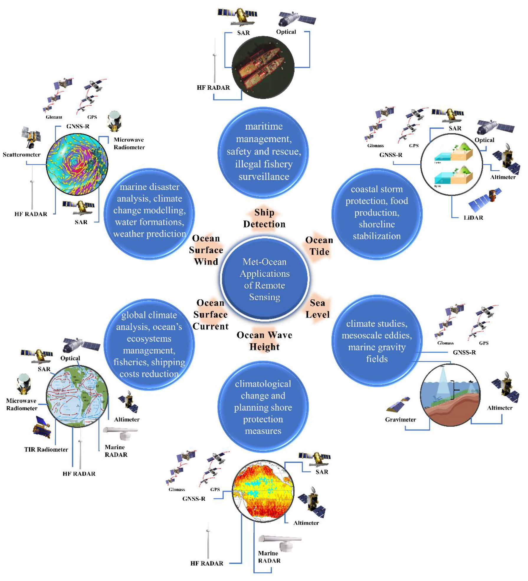
3. RS Applications in Ocean

As discussed in the Introduction, six oceanographic applications of RS are explained in Part 1 of this review paper. These applications, along with the RS systems which can be used to study them, are illustrated in Figure 1. More detailed discussions are also provided in the following six subsections.

3.1. Ocean Surface Wind (OSW)

OSW is an essential parameter for various applications, such as marine disaster monitoring, climate change modeling, water mass formations, and Numerical Weather Prediction (NWP) [76,77,78,79]. Considering the limitations of the traditional methods for OSW estimation (e.g., anemometers and buoys) [76,80], RS observations have emerged as cost-effective techniques [81]. Remotely sensed OSW information mainly relies on the relationship between the OSW and the sea surface roughness, which represents emissive and reflective properties of the ocean surface [79]. Five RS systems have been frequently applied to measure OSW: microwave radiometer, GNSS-R, SAR, scatterometer, and HF radar. The advantages and disadvantages of each system, summarized in Table 1, are discussed in more detail in the following subsections.

3.1.1. Microwave Radiometer

Microwave radiometers can estimate OSW based on the spectrum of the microwave radiation emitted by the ocean surface [79,82]. OSW measurements from microwave radiometers mainly rely on the physical RT models, which estimate the microwave emission from the ocean surface and the emission and absorption by the Earth’s atmosphere [83]. As discussed, the nonpolarimetric microwave radiometers (e.g., Advanced Microwave Scanning Radiometers (AMSR)) can only estimate OSW speed. However, the WindSat polarimetric microwave radiometer can provide both OSW speed and direction [79]. Polarimetric microwave radiometers contain ±45° polarized and right/left circularly polarized channels along with vertical and horizontal polarizations. Polarimetric microwave radiometers retrieve OSW speed and direction by measuring the complex correlation between horizontally and vertically polarized microwave radiations [32]. In fact, the difference between horizontal and vertical polarizations is related to OSW speed, and the complete state of polarization is related to OSW direction [82]. The OSW direction from polarimetric microwave radiometer systems becomes less precise when wind speed is less than 8 m/s [81,84]. This is because the passive OSW direction signal is small in all polarizations at low wind speeds, causing noisy and inaccurate measurement of the OSW direction [79,85].
Generally, microwave radiometers provide better results in high wind speeds than other low-resolution RS systems, such as scatterometers. For example, it has been reported that in spaceborne L-band radiometers, received signals remained sensitive to increasing wind speeds up to 70 m/s [86,87]. Accordingly, some of the L-band radiometers (e.g., Soil Moisture and Ocean Salinity (SMOS) and Soil Moisture Active Passive (SMAP)) can provide a reasonable estimation of extreme OSW speeds at a coarse spatial resolution [87]. The quality of the OSW measurements from microwave radiometers is negatively affected by rain [83]. However, L-band radiometers (e.g., SMOS) are almost insensitive to the presence of rain or frozen precipitation [88]. Various OSW products have been so far generated using the data collected by different microwave radiometers. For example, Yin et al. [89] implemented a novel method to estimate OSW vector in severe weather conditions (i.e., the high precipitation environment of tropical cyclones) using WindSat data. This study used HWind data [90] as the reference dataset and evaluated the proposed methodology in 17 tropical cyclones from 2003 to 2009. The results showed that the mean difference between the retrieved OSW speed and HWind data for 17 tropical cyclones was 0.2 m/s. The Root Mean Square Error (RMSE) was also 24.2°. The authors reported that the observed RMSE value was mainly related to a time or location mismatch between the HWind analysis and the WindSat data.

3.1.2. GNSS-R

As discussed, GNSS-R is a passive RS satellite utilizing the GNSS signals to estimate the OSW speed using the L-band (frequency and wavelength around 1.5 GHz and 20 cm) [34]. GNNS-R measures multiple points over the ocean to estimate the OSW speed, and its geometry is not like a swath, individual point, or limited to the nadir direction [91]. In contrast to traditional OSW speed retrieval methods, GNSS-R has better spatiotemporal sampling due to the global accessibility of the GNNS signal, which offers greater coverage over the ocean [35]. Another advantage of GNSS-R is its lower sensitivity to small atmospheric particles and small-scale capillary waves since it utilizes a longer wavelength compared to scatterometers (i.e., wavelengths = 2–5 cm) [35]. Additionally, lower cost and lower power needed for the GNSS-R receiver are the other benefits of these systems for OSW estimation [92].
The first GNNS-R data were collected by the UK-DMC satellite between 2004 and 2005 [37]. Later, in July 2014, the second spaceborne polar-orbiting satellite (TDS-1) was equipped with the Space GNSS Receiver Remote Sensing Instrument (SGR-ReSI) to collect the reflected GNNS signals [92]. The first OSW speed estimation from the TDS-1 mission was discussed in [92]. This study suggested an OSW speed retrieval method based on the Signal-to-Noise Ratio (SNR) and GNSS-R Biostatic Radar Equation. The Meteorological Operational (MetOp) Advanced SCATterometer (ASCAT) satellite measurements were used to validate the results. It was observed that when SNR was greater than 3 dB, OSW speed could be estimated with an accuracy of approximately 2.2 m/s for wind speed values between 3 and 18 m/s [92]. In late 2016, an advanced GNSS-R receiver was installed on the CYGNSS to provide higher-quality OSW speed products [93].
Fusing measurements from multiple GNSS-R systems can improve the spatiotemporal resolution of the estimated OSW speed [94]. Retrieval of OSW speed from GNNS-R data is usually based on quantities known as observables, which are extracted from the GNSS delay-Doppler maps peak [7,13]. A series of algorithms, including the delay-Doppler map variance, delay-Doppler map average, trailing edge slope, leading edge slope, and Allan delay-Doppler map variance, have been so far introduced in [8] for OSW speed estimation from GNSS-R data. The authors also suggested a new OSW speed estimation algorithm, known as minimum variance, based on the integration of OSW data from each single observation [35]. Moreover, a new parametric Geophysical Model Function (GMF), extracted from the CYGNSS measurements, was proposed by [95] to relate the OSW speed to the two observables of the slope of the leading edge of the radar return pulse scattered by the ocean surface and the normalized bistatic radar cross-section of the ocean surface. In this study, an overall RMSE of 1.4 m/s was obtained when the results were compared with in situ data [95].

3.1.3. SAR

SAR sensors measure the Normalized Radar Cross Section (NRCS) variation from the wind-roughened ocean surface as a function of both OSW speed and direction. Accordingly, GMFs are developed to establish the relationship between OSW vector information, calibrated NRCS, and sensor viewing angles for different SAR bands and polarizations [96]. However, since SAR sensors operate with a single azimuth view, it is required to infer whether backscatter variations are related to OSW speed (along-view OSW vector component) or OSW direction (across-view OSW vector component) [81]. To resolve this issue, several different methods have been implemented, a comprehensive list of which are discussed in [97]. It is also worth noting that rain can negatively affect the OSW estimation accuracy from SAR data, and rain contamination is more noticeable at shorter wavelengths [81].
SAR systems are the only satellite-based system that can provide OSW information with a subkilometer spatial resolution (between a few meters and 100 m) [96]. However, OSW retrieval using SAR data is generally implemented at spatial resolutions of 0.5–1 km for removing speckle noise as well as filtering ocean waves and other non-wind-induced features [81]. SAR systems are efficient at both low and high winds with subkilometer spatial resolutions [98]. The cross-polarized SAR data provide a very weak incidence and azimuth angle dependency, with no indication of saturation for the strongest wind speeds (up to 75 m/s). Accordingly, these capacities have opened new perspectives for OSW speed estimation in different settings, even in tropical cyclones [98,99,100]. In this regard, Li et al. [100] analyzed 83 SAR images, captured by Radarsat-1 and Envisat from 2001 to 2010, to investigate the morphology of the tropical cyclone eye in terms of shape and size distribution. The detailed atmospheric phenomena generated within tropical cyclones (e.g., rainbands, boundary layer rolls, and arc clouds) were also explored. This study demonstrated the application of SAR data for investigating the characteristics of windstorms with relatively higher resolution. In fact, by analyzing 30 typhoons and 43 hurricanes, the authors reported that the response of ocean surface to the storm-forced winds could be effectively explored by SAR data.

3.1.4. Scatterometer

Scatterometers have proven to be efficient tools for both OSW speed and direction measurements [101,102]. A scatterometer transmits a radar pulse and then measures the returned pulse ratio from the ocean surface [103]. The differential response and the intensity of the reflected pulses determine the OSW direction and speed, respectively [82]. The main operating radar frequencies in scatterometers are Ku-band (frequency = 13.4 GHz and wavelength = 5 cm) and C-band (frequency = 5.2 GHz and wavelength = 2 cm). Scatterometers provide global OSW vector information with spatial resolutions between 25 and 50 km, which is almost similar to that of microwave radiometers [79]. Unlike SAR systems, the low spatial resolution of these two instruments cannot effectively satisfy several local applications, such as tropical cyclone analysis and coastal OSW mapping. For low OSW speeds, scatterometers provide more reliable information compared to microwave radiometers. However, scatterometers lose sensitivity, and the signal begins to saturate, at high wind speeds (above 35 m/s) [104]. Like SAR systems, the rain contamination in scatterometers’ OSW measurements is more serious in the higher frequencies.
Many studies have so far investigated the potential of different scatterometers for OSW estimation. For example, Guo et al. [103] examined the spatial variability of global OSW resources at heights of 10 m and 100 m above Sea Level (SL) using multiple scatterometers, including Quick SCATterometer (QuikSCAT), ASCAT, and WindSat (see Figure 2). The authors also compared the results with mean OSW speeds and wind power densities collected by buoys during 1995–2015. Based on the results, although OSW information retrieved from each of these three scatterometers was fairly comparable, a combination of these instruments provided better results. Furthermore, other types of sensors, including terrestrial laser scanners, SONAR, and Autonomous Underwater Vehicles (AUV), have been utilized to collect data about the position, geometry, and morphology of icebergs [26,27]. Although the abovementioned approaches provide accurate information, they are resource-intensive and logistically arduous in oceans, especially in remote locations of polar regions [28]. Consequently, it is efficient to employ other RS systems, such as satellites, which can provide broad observations about the icebergs through space and time. Various RS systems have been so far applied to identify and track icebergs [10,29,31]. Optical, SAR, scatterometer, altimeter, and HF radar systems have been widely used for iceberg studies.

3.1.5. HF Radar

As discussed, HF radars measure ocean surface parameters, such as OSW speed, in a timely fashion over relatively larger areas and at a reasonable cost compared to in situ measurements. OSW speed can be extracted from either the first-order radar backscatter or the second-order sea echo. Stewart and Barnum [105] revealed that the 10-dB width of the first-order resonant scattering could be used for the estimation of the local OSW speed. However, this method was not a robust solution since it depended on different ocean parameters, such as OSC [106]. The second-order scattering is also employed to calculate the OSW speed because the amplitude of the second-order radar backscatter and its location in Range-Doppler is greatly dependent on the local OSW speed [107]. In other words, by increasing the wind speed, the second-order peaks increase and move to the first-order peaks. Moreover, Barrick et al. [108] postulated that the ratio of the second-order peak amplitudes to the first-order ones could be used for measuring the local OSW. Ahearn et al. [109] also suggested that the ratio of the second-order continuum closer to zero Doppler to the amplitude of the first-order resonant peak can be employed for OSW speed measurement because short waves represented in this region reflect the OSW speed. Additionally, Dexter and Theodoridis [110] proposed a method to calculate OSW speed from the significant OWH and period. Subsequently, Huang et al. [111] applied this method to an HF radar installed in the Eastern China Sea.

3.1.6. Summary and Future Direction

OSW is among the key components of ocean/atmosphere circulation. Accordingly, accurate knowledge of OSW is of substantial importance to understand and quantify different ocean-related characteristics. Despite the tremendous progress in the utilization of RS technology for quantitative and qualitative assessment of OSW, there are still different issues and challenges that need to be addressed in future research. These include but are not limited to improving the measurement accuracy and consistency of OSW products by integrating different data sources (e.g., buoys, satellite, and NWP), proposing novel automatic and/or semiautomatic methods for concurrently retrieving OSW and other related parameters (e.g., ocean currents and precipitation), developing new RS sensors to enhance the temporal resolution and spatial extent of global OSW products, integrating active and passive sensors to provide OSW products in all-weather conditions with the highest accuracy, and employing downscaling methodologies to enhance the temporal and spatial resolutions of OSW products.

3.2. Ocean Surface Current (OSC)

OSC is the continuous and directional movements of the mass of the seawater, transferring nutrients, energy, heat, pollutants, and chemical substances around the world [112,113]. Ocean currents affect the global climate, the ocean’s ecosystems, and fishing productivity. More importantly, they play a key role in reducing shipping costs, fuel consumption, as well as developing policies for preventing natural disasters [112,114]. OSC can originate from a wide range of factors, such as wind, Coriolis effect, water density variation, Ocean Tide (OT), as well as SST and OS differences [112,113,115,116]. The seafloor and shoreline topography can also affect OSC and hinder or boost the mixing and passageway of water from different areas [117]. Ocean currents can be generally divided into five categories: (1) geostrophic ocean current, which is balanced under pressure gradient force by the Coriolis effect; (2) tidal ocean current, which is created by the gravitational force of the moon, sun, and Earth; (3) wind-driven Ekman ocean current, which is created by the steady ocean wind; (4) wave-induced Stokes drift, which is characterized by the difference between the average Lagrangian flow velocity of a fluid parcel and the average Eulerian flow velocity of the fluid at a fixed position; and (5) small-scale ocean current, which is created by the small features such as eddies, fronts, and filaments [118]. Ocean currents are also separated into two groups based on their temperature: warm and cold ocean currents (see Figure 3) [3]. For instance, the Gulf stream, Kuroshio, and the Agulhas are warm currents that transport heat from the tropics poleward and significantly affect the global climate [112,119,120]. The Humboldt, Benguela, and California are cold currents that preserve highly upwelling waters and carry cold water toward the equator [112,120]. For example, the Labrador Current has a cooling effect with a low OS and is known for transporting icebergs from Greenland’s glaciers into shipping lanes in the North Atlantic [120,121].
Ocean currents can also be categorized into two groups according to their depth: surface and deep (subsurface) [112,118,122]. The surface currents are horizontal water streams that occur on local to global scales, and their effects are primarily restricted to the top 400 m of ocean water [112,123]. Along the coasts and offshore regions, there are local surface currents, which are typically small and short-lived (e.g., hourly/seasonal), generated by OT, waves, buoyant river plumes, and local-scale winds [112,123]. These currents control the local flooding, algal bloom, marine pollution, sediment transport, and ship navigation [112,123]. The global surface currents (e.g., the Gulf Stream) are typically controlled by dominant global winds (e.g., trade winds and the westerlies) together with Coriolis force and the restriction of flow by continental deflections [112,114,123]. These currents travel over long distances in the same direction as the wind and at a speed of approximately 3 to 4% of winds’ speed [112,123]. However, the Coriolis force deflects these currents from the equator to the right direction in the Northern Hemisphere and the left in the Southern Hemisphere, which creates the clockwise and counterclockwise circular patterns or gyres, respectively [112,114,115,123,124]. In contrast, the deep ocean currents are vertical streams under the influence of the thermohaline circulation generated by water density differences and depend on temperature and OS [112,125]. Deep ocean currents are formed with upwelling and downwelling directions below 400 m of the surface water [126].
Depending on the scale of the ocean currents, they are measured by different methods. Figure 4 illustrates various in situ and RS methods for ocean current estimation. It should be noted that the focus of this section is on the OSC using offshore, shipborne, and spaceborne platforms. Table 2 also summarizes these systems along with their advantages and limitations for OSC studies. More details about the applications of each system are also provided in the following subsections.

3.2.1. Optical

Optical satellites provide high/medium spatial resolution and multitemporal and multispectral images for oceanographic studies over large areas [112,127]. These images are typically captured in the visible (Red/Green/Blue) (0.4–0.7 µm) and Near-, Mid-, and Far-Infrared (0.7–3.5 µm) spectral ranges, and can be directly/indirectly used to investigate the spatiotemporal characteristics of OSC [112,127]. For example, OC products of optical satellites can be indirectly applied to estimate the OSC [112,116]. For instance, Sun et al. [128] employed two matching algorithms, including area-based cross-correlation and feature-based optical flow approaches, to estimate OSC from OC image pairs. The results demonstrated a high similarity between the derived OSC and the Ocean Surface Current Analysis Real-time (OSCAR) products. It was also observed that the robust optical flow method outperformed the Maximum Cross-Correlation (MCC) algorithm in terms of accuracy. Furthermore, optical RS images can be directly used to retrieve surface wave directional properties and OSC characteristics. For instance, Yurovskaya et al. [127] developed a new technique based on cross-spectral phase estimation to directly retrieve OSC and the characteristics of propagating ocean surface waves from Sentinel-2 images. The results showed that the retrieved OSC was well-matched with medium-resolution OSC models as well as the derived velocities from altimeter observations in deep ocean regions. The results over shallow water areas demonstrated that the retrieved wave propagation characteristics corresponded well with the sea-depth variations. These results confirmed the high potential of optical images in direct estimation of OSC velocity.
Although the optical satellite images are rich in content and are easy to use for OSC mapping, they are sensitive to cloud cover and are not suitable for nighttime. Moreover, the long revisit time and inappropriate latency of some optical datasets have made some of them unsuitable for real-time OSC measurements.

3.2.2. TIR Radiometer

In order to retrieve SST, Low Earth Orbit (LEO) and geostationary satellites acquire TIR data in the 7–14 µm region of the spectrum [129]. The derivations of SST from TIR satellites are typically utilized to estimate the OSC velocity by tracking the motion of natural surface features (e.g., oil and algae) in cloud-free images [112,129]. This tracking scheme is mainly carried out by analyzing the sequential TIR images in both human interactive and automatic methods [129]. In this regard, automated feature-tracking methods are more interested in retrieving OSC velocity due to the costly and time-consuming procedure of the human interactive approaches [130]. To this end, the feature tracking methods based on the MCC matching algorithm have provided promising results for NRT estimation of OSC velocity fields from consecutive TIR images [112,129,130,131]. For example, Heuzé et al. [130] used the MCC method to track features from 224 pairs of sequential TIR images acquired by Advanced Very High-Resolution Radiometer (AVHRR) between January and December 2015 in the western Mediterranean Sea. The results indicated that the satellite-based OSC resulted from tracking a small pattern with low speed and concurred well with in situ measurements, especially in summer times. Like optical satellite images, TIR radiometers are restricted by the cloud cover and undesirable viewing conditions, which reduce the spatial and temporal coverage of the resulting OSC velocity products [130].

3.2.3. Microwave Radiometer

SST and OSW measurements derived from microwave radiometers can be used to study OSC [112,132]. Compared to TIR radiometers, the coarse spatial resolution of microwave radiometers reduces the performance of sequence image analysis and MCC techniques for OSC estimation [133]. To resolve this issue, the Surface Quasi-Geostrophic (SQG) theory and multifractal analysis have been employed to retrieve OSC from a single SST microwave image [133,134]. To this end, the OSC can be reconstructed by converting the SST map to OWH using a transfer function obtained by the multifractal analysis or SQG approach [135]. In the multifractal analysis, the fact that SST multifractal structures are closely related to OSC is considered, and reasonable stream function approximation is allowed [133,134]. However, this technique cannot provide information on OSC orientation. In contrast, the SQG approach can reconstruct the 3D OSC field and is more commonly used by researchers [134]. For example, González-Haro and Isern-Fontanet [132] assessed the OSC, reconstructed from SST, using the SQG method at the global scale. The results indicated that the retrieved OSC could be improved by providing information on the energy spectrum of altimetry data.

3.2.4. SAR

SAR images are being widely used to map OSC dynamics and their variability in any weather conditions and at any time of day/night [116,122,136]. SAR-based OSC estimations are mainly obtained using two approaches: (1) feature tracking and (2) Doppler-based techniques [136]. The feature tracking methods compare sequential SAR images by measuring a similarity measure (e.g., correlation) between those images [137]. In the best case, the outputs of these methods have the same spatial resolution as the SAR images. On the other hand, the Doppler-based techniques can be divided into two groups based on their design, implementation, and performance: (1) the Doppler Centroid Anomaly (DCA) and (2) along-track InSAR [136]. The DCA methods model OSC at a coarse resolution (e.g., 1–2 km) with only one SAR image and are based on the Doppler shift concept [136,138]. These methods estimate OSC by determining the line-of-sight rate of the scatterers based on the Doppler shift [112,139]. On the other hand, along-track InSAR techniques are widely utilized to generate high-resolution OSC maps with two SAR images [136]. The spatiotemporal decorrelation and atmospheric delays strongly reduce the performance of these methods. Therefore, it is necessary to select multitemporal SAR images with appropriate temporal and spatial baselines to achieve better results from these methods. Multiple studies have investigated the potential of SAR-based methods for OSC retrieval. For instance, Fu et al. [140] proposed a new technique to provide maps of shallow water topography and OSC using SAR images. In this method, OSW and OSC were estimated by fitting the observed SAR signals to a simulated shallow water topography radar signal in an iterative procedure. The results showed the high efficacy of the proposed methods. Moreover, Elyouncha et al. [141] investigated the potential of Sentinel-1 SAR data for OSC mapping in the Skagerrak Sea with a focus on the Norwegian Coastal Current. They implemented several postprocessing algorithms for scalloping removal and the absolute and interbeam bias correction in the Sentinel-1 data. The results showed that the retrieved OSC velocity corresponded well with a regional ocean circulation model with values of ≈0.8 m/s.

3.2.5. Altimeter

Altimeters with Ku-band (13.8 GHz) also provide information about the large-scale dynamic topography of the ocean, particularly OWH and OSW speed, which can be directly used to estimate the global OSC and its variability at coarse spatial resolutions (e.g., 10 km) [112,135,142]. Moreover, integrating altimetry data with tide-gauge data and hydrodynamic models increases the knowledge about global OT and OSC variability [136,142]. However, altimeters cannot measure the non-geostrophic components of the OSC due to non-geostrophic and local winds [136]. Several efforts have been made so far to derive OSC from altimetry data. For example, the NRT Archiving, Validation, and Interpretation of Satellite Oceanographic (AVISO) products, as geostrophic OSCs, have been generated by integrating the satellite altimetry and precise satellite position data and are available at a global scale (see Hwang and Fan [90] for more information). Moreover, the OSCAR project, developed by the National Oceanic and Atmospheric Administration (NOAA) [112,113,114], and the GlobCurrent project, developed by European Space Agency (ESA) [90], provide the complementary information for AVISO products in reliable estimating of the Ekman component of the OSCs [118].

3.2.6. HF Radar

Over the last few decades, HF radar systems have been successfully employed to remotely measure coastal and offshore currents using the concept of Bragg-scattering [112,122,143]. The local currents can be typically measured by a land-based radar antenna pair over a wide area, up to 200 km or more, and with coarse spatial resolutions (e.g., 0.5–6 km), according to the selected HF radio band, which could be in the range of 3 to 45 MHz [122,136,143]. Consequently, HF radar systems, as a cost-efficient tool, cover a wider range than marine radars (i.e., X-/S-band radars) [112]. Moreover, HF radar systems are typically preferred over marine radars to support the worldwide monitoring of marine and coastal ecosystems, although they cannot produce high-quality data such as X-band image sequences [79]. For example, there is a global HF radar network operating throughout the world to produce continuous maps of local OSCs (see Figure 5) [90]. This network provides NRT measurements of OSC fields which are applicable for operational marine services, coastal marine studies, OOS detection, water quality assessment, pollution tracking, search and rescue, and numerical ocean forecasting models, especially near the coast [79,144]. Various studies have so far investigated HF radar data for OSC estimation. For example, Ji et al. [145] investigated the capability of the HF Hybrid Sky–Surface Wave Radar (HFHSSWR) for OSC estimation. The results were compared with in situ measurements from a current meter, and it was observed that there was a good agreement between HFHSSWR results and in situ data, with a correlation coefficient of 0.81 and an RMSE of 0.138 m/s.
The high sensitivity of HF radar signals to sea surface topography and electromagnetic interference from different sources, as well as data acquisition failures, causes frequent gaps in HF radar data, which is the main limitation in utilizing these datasets for continuous OSC retrieval [146]. To resolve this, Kolukula et al. [146] presented a gap-filling algorithm for HF radar data using the complex empirical orthogonal functions and validated it using two datasets with different gap rates. The results showed that the method had high efficacy in reconstructing data. The direction pattern and magnitude of the reconstructed data were well-matched with the existing data.

3.2.7. Marine Radar

Over the last four decades, marine radars, deployed on ships or land, have been widely employed for OSC [112,147]. In most studies, the X-band radars were preferred to S-band systems due to their clear sea-clutter images [148]. However, X-band radar data are more sensitive to interference from raindrops; thus, this radar frequency is mostly used by weather surveillance radar for rainfall monitoring [148,149]. Marine radars scan the sea surface at close ranges (i.e., limited by line-of-sight propagation to the horizon) with relatively high spatial (~9 m) and temporal resolutions [73,147,148] to derive OSC. The Wave and Current Analysis and Wave Spectra (WaMoS) II, developed by the OceanWaveS GmbH company, is an example of an operational system that works based on X-band [73,150]. The WaMoS II system measures and displays wave (e.g., peak wavelength and direction) and OSC parameters (e.g., OSC speed and direction) [73]. These measurements are mainly obtained by taking a sequence of X-band radar images and analyzing the subsequent waves [73,150]. Figure 6 demonstrates a scheme of a WaMoS II X-band radar installation and its images, along with bathymetry and OSC field.
Hessner et al. [73] investigated ocean wave variations and OSC characteristics by the WaMoS II High Resolution Current (HRC) at Tongue Point, New Zealand, during August 2011, using three scenarios based on high, low, and slack tides. The results showed that the WaMoS II HRC data had high efficiency in detecting small-scale OSC features and could demonstrate the influences of the OT and local bathymetry interaction on the diversity of current patterns. Furthermore, Chen et al. [72] improved the cross-spectral approach to estimate the velocity of OSC from the X-band image sequences. The results indicated that the estimated current velocity had a more acceptable accuracy compared to the current velocities measured by a current meter, with a correlation coefficient of 0.88 and a relative error of 7.79%. However, conditions such as the sampling period of one to three seconds, and radar image acquisition within 10 to 40 s, were necessary to obtain reasonable results.

3.2.8. Summary and Future Direction

In summary, HF radar has widely been applied to estimate coastal and offshore OSC, while altimeters have mostly been used to measure global OSC. However, the range of the HF radars was limited to between 200 km to 600 km, which should be further improved to obtain more accurate information from coastal OSC. Moreover, HF radar and altimeters observations have data gaps (no data) due to the presence of obstacles, such as artificial features (especially for HF radar) and atmospheric conditions and clouds (especially for radiometers). Integrating these datasets with in situ data and OSC derived from TIR/Microwave radiometers and SAR systems could help reduce the gaps and improve the accuracy of the OSC map.
Although the airborne RS systems provide high spatial resolution data for ocean applications compared to spaceborne systems, they have been rarely used for OSC estimation due to their high cost and lower coverage over ocean. The gap between spaceborne and airborne RS data has been recently filled by data derived from Unmanned Aerial Vehicles (UAVs). UAVs can provide affordable observations with very high spatial and temporal resolutions for OSC estimation and monitoring. Moreover, various sensors (e.g., optical, SAR, and LiDAR) can be mounted on a UAV to collect data over the ocean. Such multisource observations can drive new developments in the OSC estimation. RS CubeSats (i.e., mini satellite systems from 1 to 100 kg) have also created a paradigm shift in ocean applications by providing data with high temporal and spatial resolutions. These observations can efficiently be utilized to monitor a wide variety of ocean parameters describing the OSC.

3.3. Ocean Wave Height (OWH)

Wind blowing over the ocean surface creates ocean waves with a different range of heights depending on the wind speed, wind duration, and distance. The resulting waves can travel for hundreds or even thousands of kilometers and form swell waves of various heights. Although waves are generally caused by wind, catastrophic waves (e.g., landslide surges, tsunamis, and storm surges) [151] and internal waves (e.g., subsurface waves at the boundary between two water layers) [152] can also generate ocean waves. OWH information is a critical parameter for coastal construction, ship navigation, and human activities in the oceans [153].
The datasets collected by different RS systems, such as GNSS-R, SAR, altimeter, and marine radar, have been utilized for OWH estimation. In this regard, various models have been applied to retrieve OWH from these datasets [154]. For example, due to the complexity of physical models (e.g., RT models), empirical and semiempirical models have also been developed to estimate OWH [155]. The simplicity of empirical and semiempirical models has also led to the development of ML algorithms [156]. In this regard, DL algorithms, as the most advanced ML models, have received more attention due to their promising performance. For example, Shao et al. [157] proposed a hybrid statistical and a DL model in South China to predict several ocean surface variables, including OWH. In Liu et al. [158], a short-term memory deep network was also proposed to consider the time domain data in OWH estimation. Table 3 summarizes the advantages and disadvantages of each of these RS systems. In the following subsections, the studies that have been conducted to measure OWH based on various RS systems are discussed in more detail.

3.3.1. GNSS-R

Various GNSS-R techniques using either single or double antennas, as well as direct or reflected signals, have been proposed for OWH estimation. The signal arrival time was also used for OWH estimation in Rius et al. [159]. The recorded SNR ratio was first used for OWH measurement by Chen et al. [160] in 1995. Later, Larson et al. [161] and Santamaría-Gómez et al. [162] successfully showed the robustness of the proposed method in [160] for OWH estimation. Moreover, Penna et al. [163] used a GNSS Wave Glider (GNSS WG) through a 13-day experiment to measure OWH in the North Sea. Their results showed that GNSS WG could address the challenges of coastline-based tide gauges for OWH measurement, and the temporal and spatial resolution limitations of radar data.

3.3.2. SAR

SAR is a unique system for OWH observation from space because it has a high spatial resolution (e.g., 1–10 m), broad coverage, and it is independent of cloud cover and light conditions [164]. SAR uses the omitted backscattering signal from the ocean surface to measure OWH [165]. Theoretical and empirical algorithms are two main techniques that have been employed for OWH estimation using SAR images [166]. Theoretical algorithms, standing on the SAR wave mapping mechanism (i.e., nonlinear velocity bunching, tilt modulation, and hydrodynamic modulation), invert the SAR intensity spectrum into a wave spectrum [167]. The semiparametric retrieval [168], parameterized first-guess spectrum [169], and partition rescaling and shift [170] are three well-known theoretical-based algorithms for OWH estimation using SAR data. On the other hand, empirical algorithms, which do not need prior information of wind and wave, can directly estimate OWH from inputs generated from SAR images [171]. C-band WAVE models for European Remote Sensing (ERS)-2 [172], Envisat [173], and Sentinel-1 [174], as well as the X-band WAVE model [175] for TerraSAR-X, are some examples of the empirical algorithms.
Among SAR systems, Sentinel-1, which provides open-access imagery with dual-polarization, has been widely used for OWH estimation. For instance, Shao et al. [176] used a semiempirical algorithm along with Sentinel-1 imagery (C-band VV-polarization) for OWH retrieval. The results illustrated that the algorithm could successfully estimate OWH with an RMSE of 18.6.

3.3.3. Altimeter

Generally, altimeters measure the traveling time (T) of the transmitted radar pulses at regular intervals defined by the Pulse Repetition Frequency (PRF) from a nadir-pointed antenna to the ocean surface and back to the receiver onboard the satellite, according to the following equation:
T = 2 R c
where c is the speed of light and R is defined as the range from the sensor to the ocean surface. R can be calculated using Equation (2).
R = 1 2 c T
R is an uncorrelated range and should be modified based on Equation (3) to take into account various ranges of atmospheric and geophysical corrections, including wet and dry tropospheric correction, ionospheric correction, and solid and pole earth tide correction [177].
R c o r = 1 2 c T i Δ R i
where Δ R i is related to the aforementioned range corrections. The data collected by Jason-3, Chinese HY-2A/B, Satellite with ARgos and ALtiKa (SARAL), and Sentinel-3 altimeters have been widely used in OWH estimation. These satellites offer global observations under all weather conditions [178]. For example, Wang et al. [178] estimated OWH based on observations from HY2B. They used the data collected by the National Data Buoy Center (NDBC) from April 2019 to April 2020 for validation purposes. In this study, numerous DL algorithms were utilized to approximate the waveform of HY2B with high accuracy. Moreover, Peng and Deng [179] enhanced the Brown model to estimate OWH based on three years of observations from the Jason-1 data. The results were validated against observations from eight buoys and compared with the retrieved OWH by the four-parameter Maximum Likelihood Estimator (MLE) retracing method. Moreover, SARAL (i.e., the first Ka-band altimeter) observations were used to retrieve the OWH in the coastal ocean and inland water bodies. Validation of the results with the in situ measurements demonstrated a significant correlation (0.98) between field measurements and satellite measurements in the coastal ocean; the performance was remarkably stable across various coastal zones.

3.3.4. HF Radar

HF radar is another RS system to measure OWH. This parameter can be calculated based on the first- and second-order sea surface scattering mechanism. Generally, OWH depends on the integral of the second-order part of the radar-measured Doppler spectra [180]. Beamforming is required to obtain the OWH over various ranges and azimuths. Thus, a narrow-beam system along with a large aperture is essential for retrieving a wave map using HF radars [181]. In this regard, Tian et al. [182] proposed a method to calculate OWH based on the second-order harmonic peaks of radar Doppler spectra and its ratio to the Bragg peak power. The comparison of the results with buoy data over a 30-day experiment depicted that the RMSE was between 0.33 and 0.77 m. It is worth mentioning that the second-order scattering is vulnerable to the external clutters and noise which may reduce the robustness of the OWH measurement [183,184,185]. On the other hand, the first-order radar backscatter has stronger power compared to the second-order harmonic peaks. In this regard, Zhou and Wen [186] proposed an empirical method to calculate OWH from the power of the first-order peaks. Subsequently, Tian et al. [187] proposed a technique using the power ratio of the first-order peaks acquired at two radar frequencies to estimate OWH. By utilizing the first-order peaks instead of the second-order peaks to calculate the OWH, the detection range improves because of the high SNR value. Nevertheless, this method can be affected by low sea state conditions due to the saturation of the Bragg waves [182].

3.3.5. Marine Radar

Since the 1980s, marine radars have been mainly developed to measure ocean surface parameters such as OWH. This is because of their high temporal and spatial resolutions as well as the distinguishability of ocean waves in the corresponding images [188]. Several texture-analysis-based, spectral-analysis-based, and coherent radar algorithms have been so far developed for OWH estimation using marine radar data.
Spectral-analysis-based algorithms acquire wave spectra information from a series of radar images to generate OWH information. These methods can be generally divided into three groups, namely, the 3D discrete Fourier transform-based algorithms [189,190], 2D continuous wavelet transform-based algorithms [191], and the array beamforming algorithms [192]. Regarding texture-analysis-based algorithms, wave parameters are directly generated from image texture information based on seven different methods, including the probability of illumination [193], statistical analysis [194], tilt-based [195,196], shadowing-based [197], support vector regression [198], empirical orthogonal function [199], and ensemble empirical mode decomposition [200]. Finally, coherent radar algorithms have been developed based on the X-based coherent marine radars [201]. The image intensity and the radial velocity of the ocean surface scatters are two main advantages of coherent marine radars. These systems enable coherent radar-based algorithms to directly estimate OWH information from the radar data without calibration [188]. Based on this feature, several empirical [202], semiempirical [203], and nonempirical [204] methods have been developed for OWH estimation.

3.3.6. Summary and Future Direction

Most of the OWH studies using RS datasets have focused on data or algorithm-driven solutions, but the quality assessment of airborne/spaceborne-derived OWH under a variety of conditions has been investigated less. Moreover, application of advanced ML algorithms in analyzing, interpreting, and modeling RS data has received less attention from researchers, even though they can offer a great potential for accurate OWH mapping and monitoring tasks. For example, DL algorithms have rarely been used to model and estimate OWH from RS data, while they have significantly outperformed traditional methods by relying on their ability to train models with massive datasets. Indeed, DL methods can significantly facilitate understanding the complex structure of large RS data for OWH estimation/prediction.

3.4. Sea Level (SL)

SL is an important oceanographic variable that should be measured precisely for long-term trend assessments and climate studies [205]. SL has a pivotal role in studies related to OSC, mesoscale eddies, and marine gravity fields [206,207,208]. In recent decades, anthropogenic activities and global warming have mainly resulted in SL change. For instance, the Intergovernmental Panel for Climate Change (IPCC) reported a Global Mean SL (GMSL) rise of 3.6 mm/yr between 2006 and 2015 [209,210]. However, the relative rate of SL change is not globally identical because it depends on different spatial and temporal parameters (see Figure 7).
Conventionally, SL estimation was based on coastal monitoring stations, tide gauges, buoys, and ship surveys [212]. However, the high cost and sparse observations of these approaches make them inappropriate for SL measurements in most cases. Moreover, in situ measurements contain significant interannual and decadal effects and do not perfectly manifest the SL change [213]. However, with the advancement of RS technology, satellites provide valuable datasets to study SL at different local to global scales. In addition to studies that only focused on SL measurements using RS systems, many studies related SL observations to different environmental variables. Through these analyses, it was widely argued that the main contributors to SL rise are thermal expansion of seawater [214], Antarctic and Greenland ice sheet melting [215], and land-water storage change due to the groundwater depletion [216]. Consequently, SL rise has many environmental and economic impacts, including reef island destabilization [217], wave resource alteration [218], coastal erosion [219], saltwater intrusion into aquifers [220], sea turtle nesting threatening [221], lowland and delta vulnerability [222], coastal flooding [223], seaport infrastructure susceptibility [224], wetland inundation and displacement [225], island and offshore baseline loss [226], tidal dynamics [227], and length-of-day changes [228].
Among different RS systems, GNSS-R, altimeters, and gravimeters have been widely employed for SL studies [229,230,231,232,233]. The advantages and disadvantages of these systems applied for SL mapping are provided in Table 4. The following subsections discuss the applications of each system.

3.4.1. GNSS-R

GNSS-R systems use direct or reflected GNSS signals to measure the SL. To this end, different techniques, including floating carpet boats [234], unmanned surface vehicles [234], and spaceborne/airborne GNSS-R [235], can be employed. The first two approaches carry the GPS antenna to directly compute the elevation value of the corresponding instrument, which is then converted to SL. These approaches are only suitable for relatively small regions. On the other hand, GNSS-R employs reflections of signals transmitted from navigation satellites to infer several geophysical parameters [236,237]. GNSS-R can provide SL data at a global coverage with high spatiotemporal resolutions [212,229]. The concept of GNSS-R relies on measuring the delay between direct and reflected signals reaching the receiver (e.g., aircraft, satellite) above the ocean. In particular, the computed delay waveforms (from delay Doppler maps) enable the estimation of the SL through geometric models [238]. It was reported that the nominal precision of SL measurement from an individual 1-s GNSS-R was 5 m [239]. Further enhancements, such as employing more observations from multiple GNSS-R data over more time ranges, could improve the precision to about tens of centimeters [240]. For example, Qiu and Jin [212] employed the data acquired by the eight satellites of the CYGNSS mission to estimate the GMSL. The calculated GMSL was validated by satellite altimetry and the DTU-10 sea surface model. The results showed a significant correlation of 0.97 with both datasets, demonstrating the high potential of the CYGNSS for global SL measurements. Likewise, Wang et al. [241] implemented different ML algorithms to retrieve SL from GNSS-R data. They reported that the ensemble of ML algorithms, along with three input features (i.e., the 70% peak correlation power, peak first derivative, and leading-edge slope) from airborne delay waveform dataset, led to the best results, with an RMSE of 0.23 m concerning the DTU15 model.

3.4.2. Altimeter

The first generation of altimeters measured SL at the nadir angle along the ground track with low spatial resolution. Consequently, it was required to merge obtained data of multiple acquisitions to provide full coverage over relatively large study areas. Therefore, they had limitations in estimating SL at the mesoscale and short time intervals [229,237]. Moreover, the low spatial resolution of traditional altimeters and the waveform tracking effect at the sea–land boundary made these systems less applicable to near-shore regions [48]. To overcome these shortcomings, new principles were introduced to obtain high-resolution and wide-swath altimetry data. These new principles resulted in the invention of SAR and InSAR altimeters [49,50].
Generally, preprocessing (e.g., orbital correction and outlier observation removal) and geophysical correction (e.g., dry/wet tropospheric correction, sea state bias correction, dynamic atmospheric correction, ionospheric correction, and tidal effect correction [242,243,244,245,246]) steps are required to prepare altimetry data for further SL studies. For example, Ren et al. [247] employed the Chinese Tiangong-2 Interferometric Imaging Radar Altimeter (InIRA) data to measure SL. The results were compared with one-dimensional SL data from previous altimeters of Jason-2, SARAL, and Jason-3. Then, the observed systematic and parametric biases were analyzed and removed to obtain a standard deviation of 8.1 cm in OWH estimation, indicating the promising results of the InIRA SL measurements. Additionally, Dinardo et al. [248] investigated the potential of the CrySat-2 SAR altimetry for SL retrieval along the coasts of the German Bight and West Baltic Sea. The computed SL values were compared with in situ and regional models between 2010 and 2016. Their results showed an acceptable consistency with the regional ocean model, with a standard deviation of the differences of 24 cm. Finally, Mullick et al. [249] investigated the coastal vulnerability of Bangladesh using the Composite Vulnerability Index (CVI). To this end, satellite altimetry data from TOPEX/Poseidon (1992–2006) and Jason 1–3 (2006–2017) were combined with other parameters (e.g., land use, mean tidal range) to map the CVI along Bangladesh’s coast. It was observed that 16% of the total coastline (87 km) was highly vulnerable. Finally, Yang, et al. [250] developed a fusion approach based on deep belief network to integrate satellite altimetry and tide gauge data. The results revealed that the proposed method performed well when limited along-track altimetry and gauge data are available. Furthermore, it was observed that the distribution of altimetry and gauge datasets had a lower impact when the deep belief network was implemented.

3.4.3. Gravimeter

Ocean mass and steric changes cause variation in SL [251]. The ocean mass is associated with exchanges of ice and water mass with oceans, affecting the regional and global gravity. Therefore, it is possible to measure SL changes through gravimeters [252]. For example, the GRACE mission observes the Earth’s gravity, enabling the measurement of GMSL change associated with ocean mass alterations [253]. Although GRACE provides global coverage of the Earth’s gravity, it is difficult to employ it for regional studies due to the existing uncertainties in low spatial resolution gravity data [230]. For instance, Jeon et al. [230] applied RL05 GRACE monthly data provided by the Center of Space Research (CSR) and the GeoForschungsZentrum (GFZ) in Potsdam to quantify the global SL change. The atmospheric and ocean de-aliasing model was also used to remove the contributions of atmospheric surface and ocean bottom pressures. Finally, the gravity observations revealed a GMSL rise of about 2.14 ± 0.12 mm/yr. Additionally, Elsaka et al. [254] employed satellite gravimetry and altimetry data to evaluate the Nile Delta–Mediterranean Sea interactions. Gravity observations, acquired from GRACE, revealed an erosion rate over the eastern and western parts.

3.4.4. Summary and Future Direction

Despite the advantages of RS techniques over traditional SL mapping approaches, RS systems generally suffer from coarse spatial resolution over ocean environments. Data acquisition over an extended period is essential to obtain reliable results and to obtain comprehensive findings of SL changes. In this regard, improving the knowledge of SL either by developing more advanced RS systems with better spatial and temporal resolutions or by synergy of observations (i.e., different RS systems), consistent data acquisition, and developing advanced methodologies based on ML algorithms can assist in resolving some of the limitations of RS systems for SL studies [232,233]. In particular, employing ML and DL algorithms for accurate SL estimation should be considered in future studies due to their high potential for providing accurate SL data [158]. Furthermore, integrating SL observations acquired by different sources is highly required in order to improve our understanding of the global-to-local SL dynamics and resolve the limitations of single-source observations. Finally, the continuation of using RS observations to measure SL by developing and constructing new sensors with improved capabilities is an essential prospect [229,230,231].

3.5. Ocean Tide (OT)

OT refers to the regular rise and fall of the ocean water caused by the gravitational pull of the moon and sun in relationship with the geometric location of the Earth’s surface [255]. The cyclical effects of the Earth’s and the moon’s rotations are, respectively, the primary factors of the periodic rhythm and height of OT [256], and 24 h and 50 min is the tidal period [256]. When the water wave slowly rises to its crest (highest level), covering much of the shore, high tide occurs. Once the water wave falls to its trough (the lowest part of the wave), it is known as low tide [255,256]. Thus, the tidal range is the vertical difference between the high and low OT [256]. Ebb tide is called the flow of water from high tide to low tide [255]. During the moon’s revolution around the Earth, the direction of its gravitational attraction is aligned with that of the Sun. High spring OTs are created when the moon, Earth, and sun are in alignment. This alignment occurs every 14–15 days during full and new moons [256]. On the other hand, during the first and last quarters of the moon, neap OTs happen when the moon appears half-full [255,256]. Intertidal zones are the lands in the tidal range categorized in the splash, high-tide, mid-tide, and low-tide zones [257,258].
While traditionally, in situ measurements and numerical models have been used for OT studies, RS has been proposed to fill OT measurement gaps over the past four decades. RS technology has expanded our understanding of global OT [259,260,261] and facilitated continuous OT monitoring and predictions over wide-spread scales. RS systems can be used to study several aspects of OT, including tidal flats, tidal channels, tidal currents, Ocean Tidal Load (OTL), and tidal wetlands. In the following, a brief description of each type of OT is provided.
The area inundated between low- and high-tide waterlines is defined as tidal flats and is a mixture of seawater and freshwater environments [262]. Tidal flats provide essential services, such as coastal storm protection, food production, and shoreline stabilization [262]. A recent study has discovered that tidal flats occupy approximately 130,000 km2 of the planet (Figure 8) [263]. Murray et al. [263] also reported that about 70% of the global tidal flats occurred in three continents, namely, Asia (44% of total), North America (15.5% of total), and South America (11% of total), 49.2% of which were concentrated in eight countries, namely, Indonesia, China, Australia, the United States, Canada, India, Brazil, and Myanmar. Monitoring tidal flats using field observations is limited to estimating the ebb/flood characteristics, adequate surveys for large tidal flats, and the field access. However, RS in combination with in situ measurements facilitates monitoring tidal flats in a more cost- and time-efficient approach. In fact, RS data with a high temporal resolution are necessary for tidal flats studies because there are coastal areas that fall dry during each tidal cycle [264], and tidal flats are only exposed fully for a short period at low tides.
A tidal channel is a type of stream or a waterway that occurs during the ebb tide and flood tide in the tidal flats [265]. Tidal channel networks are crucial aspects of the neighboring ocean and estuaries. In addition to the control of the tidal basin hydrodynamics, tidal channels connect intertidal flats to the salt marshes, which play an important role in tidal propagation [266]. Due to various morphological characteristics from terrestrial river networks, conventional river system algorithms cannot be implemented on tidal channels. Thus, RS techniques have been effectively utilized to obtain the spatial distribution of tidal channels [266].
The periodic movement of water created by the out-of-phase OT, the local weather patterns (radiational tides), and ocean characteristics (internal tides) is defined as tidal currents [267]. Periodic tidal currents play an important role in the strait (a narrow waterway joining two larger water bodies) [267]. Tidal currents’ power intensifies when flowing through the narrow and shallow channels in the islands or over the shallow ridges, although they are weak in most parts of the strait [268]. Furthermore, tidal current power is renewable and predictable energy [269], mostly occurring at narrow tidal channels. Tidal current generators not only cause fewer environmental concerns than barrages, but can also be installed incrementally to meet the increase in demand over time [270]. Therefore, mapping the tidal energy density is crucial to consider the economic possibility, while tidal currents vary regionally. In this regard, a higher level of measurements, including spring and neap tidal cycles and higher temporal and spatial measurements, are required [269].
OTL displacements are the elastic response of the Earth to the redistribution of water mass from OT, which can cause deformation gradients of several millimeters to centimeters near coastal regions [271]. One of the most productive inland and coastal ecosystems is tidal wetlands. Tidal wetlands are important for trapping sediment and pollution, recreational purposes, and flood control. They are also natural barriers against saltwater intrusion into freshwater aquifers [272,273]. The tidal regime, relative SL rise, land cover change, and sedimentation are driving factors influencing tidal wetlands [274]. Tides increase rates of relative SL rise, resulting in brackish water and a shift to becoming nontidal wetlands in freshwater tidal areas. So far, different RS systems have been successfully employed for OT studies. Table 5 summarizes the advantages and limitations of the RS systems that have been frequently used for OT measurement.

3.5.1. Optical

Optical satellite images have been extensively exploited to study different aspects of OT mainly due to the availability of open-access imagery and proper temporal and spatial resolutions. For example, the Normalized Difference Water Index (NDWI), Modified Normalized Difference Water Index (MNDWI), Normalized Difference Vegetation Index (NDVI), Land Surface Water Index (LSWI), Automated Water Extraction Index (AWEI), Modified Soil-Adjusted Vegetation Index (MSAVI), and Enhanced Vegetation Index (EVI) generated from optical satellite images have been applied to delineate tidal flats by subtracting the classified images of the high and low tides [263,275,276]. Waterlines, which are important for studying changes in tidal flats and coastlines [277], can also be efficiently extracted using high spatial resolution optical satellite imagery. Appropriate spectral bands for waterline extraction must be selected based on various conditions. For instance, the NIR, SWIR, and TIR bands are efficient for flood tide [278,279].
Spatial analysis and edge detection methods in optical satellite images have also been applied to locate and map tidal channels. For instance, box-counting, a widely used fractal method, is a spatial analysis method used to identify linear features such as streams and coastlines. Moreover, a multilevel knowledge-based approach can extract channel edges using multiscale edge detection algorithms in optical images [266]. The low-level processing uses edge detection algorithms (e.g., the Sobel and Prewitt operators) to discover channel edges and then associates neighboring nonparallel edges together to form channels [266]. For example, Angeles et al. [280] proposed a fractal analysis of tidal channels using box-counting and contiguity methods for Landsat-5 data to derive the degree of geomorphological control on a tidal channel network in the Bahia Blanca Estuary, Argentina.
Finally, optical satellite data have been widely used for tidal wetland classification. To this end, various spectral and textural indexes, along with advanced ML algorithms, have been employed [272,273,281,282,283].

3.5.2. GNSS-R

GNSS-R provides range measurements, which can be used to remove vertical land motion from tide gauge records [284]. However, many GNSS-R stations are not directly collocated to the tide gauge stations. GNNS time-series have also been applied in models to remove the influence of non-OTL from GPS coordinates [285]. In this regard, the Precise Point Positioning (PPP) technique is used to process the GNSS-R data [286]. OT can cause horizontal and vertical motions of more than a centimeter during a day, which is large enough to be measured with space geodetic techniques. In this regard, Zhou et al. [286] investigated OTL displacement parameters with kinematic PPP using the harmonic analysis method from GNSS coordinate series considering the effect of mass loading.
Moreover, GNSS-R data, along with airborne RS techniques, have been utilized in a semiautomatic method to propose 3D distribution tidal channel maps including their shapes and locations [265]. The tidal channels’ volumes and locations were verified by comparing GNNS positioning solutions and the coordinates extracted from UAV images. Moreover, Lee et al. [265] generated 3D safety mapping of tidal channels located in the western coastal area in Korea, where tidal channels were considered the main cause of the summer drowning fatalities. Finally, GNNS technology has been extensively utilized to determine real-time tidal information using tidal level extraction algorithms, which can provide additional values to different aspects of OT studies.

3.5.3. SAR

SAR data have also been utilized for waterline extraction, which is an important step for studying tidal flats. This can be performed through measuring the roughness of the surface based on the differences in surface roughness between the smooth tidal flats and the water surface [287]. Thus, an efficient edge detection method should be applied to delineate the border between open water and tidal flats [288]. For instance, Heygster et al. [288] obtained the border between tidal flats and adjacent water areas by applying a multiscale edge detection algorithm using ERS-2 images. To this end, they used the computationally efficient wavelet transform method in combination with a segmentation algorithm.
Additionally, SAR data are the most popular RS resources for studying tidal currents. Thus, different SAR methods, such as radar Line of Sight (LOS), Fourier transformed images, and interferometry, have been so far implemented for tidal current studies. The components and variations of tidal currents can be found in the radar LOS [269]. Moreover, along-track InSAR has been widely applied to monitor surface tidal currents [289]. To this end, ocean waves are detected using SAR and transfer functions applied to the image spectra. Furthermore, Doppler measurements by the along-track interferometry of two SAR images can retrieve surface currents. For this purpose, phase differences between coregistered pixels of two images are obtained using the signal phase [269,289]. The phase difference is transferred into LOS scatterer velocity, and then the average effect of the horizontal wave motion is subtracted from the current field [269]. Moreover, tidal currents are mapped using equations including angular frequency, acceleration of gravity, two-dimension wave number, water depth, and the surface current [270]. MCC is another method for tidal current mapping using SAR data. Since this method cannot address the large spatiotemporal variations in a typical diurnal or semidiurnal tidal current, temporal decorrelation is minimized by a virtual SAR constellation data pair [290].
InSAR has also been used for OTL studies. Due to small changes caused by OTL, InSAR techniques are the most common RS methods for OTL studies. However, it is challenging to distinguish the OTL effects from similar signals in Differential InSAR (DInSAR) measurements. Since existing tools readily calculate the OTL effect, the OTL prediction model should be subtracted from an interferogram before tectonic analysis [291]. The dominant component of OTL displacement is vertical, and the LOS look angle of most SAR satellites makes them sensitive to vertical-ground deformation [291]. The proposed methods first accurately remove the orbit errors under the constraint of the relative displacements of the GPS PPP solutions in the LOS direction. Then, the crustal deformations caused by the OTL in DInSAR interferograms are analyzed. Finally, the OT model is applied to correct the OTL effect in the DInSAR interferograms [292]. Many studies have investigated the applications of the DInSAR technique for OTL analysis. For example, DiCaprio and Simons [291] investigated the capability of OTL correction in DInSAR using an empirical OT model to illustrate the superiority of an OT model in correcting the OTL effect in DInSAR results. The focus was on displacements from mass loading due to the OT to study processes occurring using ERS and ENVISAT data. Additionally, Peng et al. [292] measured the OTL effect as a potential error source exploiting DInSAR data and tried to use empirical models to correct the error. They proposed a linear surface model to correct the relative displacements of the GPS PPP in LOS over the Los Angeles basin. Then, an OT model was applied to correct the OTL effect in the DInSAR interferograms. It was observed that the bilinear ramp function model was in agreement with the experimental results. Finally, multitemporal SAR data have been extensively used for tidal wetland mapping [273,293,294,295]. For instance, Wdowinski et al. [293] presented the possibility of using high-resolution ALOS, RADARSAT-2, and TSX to characterize the extent of the OT flushing zone. They also provided quantitative constraints for detailed coastal wetland flow models using wetland InSAR techniques.

3.5.4. Altimeter

Satellite altimetry data have been utilized to study OT and improve the global OT models [296,297]. Furthermore, utilizing altimetry technology is one of the approaches used to detect shoreline changes over tidal flats [298]. For two decades, global SL changes were extensively studied using satellite altimetry [299]. For instance, Elachi et al. [49] estimated water level over tidal flats by analysis of the waveforms. Tseng et al. [299] also discussed the sufficiency of the coastal Digital Elevation Model (DEM) compared to current altimetry methods. The measurement of quantitative changes of tidal flats was performed by comparing the DEM produced using the waterline technique applied to SAR images and a DEM constructed from airborne altimetry data acquired in different years [300]. As discussed, satellite altimetry also enables global mapping of significant OWH, the results of which can be used for OT studies. For example, Passaro et al. [301] proposed a new algorithm for reprocessing altimetric waveforms to estimate significant OWH over a challenging tidal flat using Envisat, Jason-1, and Jason-2 data.
Satellite altimetry is highly effective in observing global tidal currents. The satellite altimetry sampling illustrates a broad view of the global distribution, variability, and spatial structures of currents. Considering the potential of tidal current energy at straits, Yu et al. [302] proposed a method to provide a global map of significant OWH. Lee et al. [303] also used TOPEX/Poseidon altimeter data as one of the inputs to model tidal currents. Additionally, Green and Pugh [304] argued that the current magnitude is underestimated in altimetry-constrained OT databases.

3.5.5. LiDAR

LiDAR data, which provide topographic data over ocean and land, are considerably helpful for OT studies. Since elevated shorelines can be detected using multiple images over a range of tide and surge elevations, DEM data generated from LiDAR systems are useful. Therefore, DEM data have been locally generated and applied along with waterline methods to detect tidal flat changes [18,29,305,306,307,308,309,310]. However, it should be noted that the coastal DEMs which are globally generated (e.g., WorldDEMTM, SRTM, and AW3D30) do not include tidal flats because of the water-impermeable nature of existing RS approaches [49].
As mentioned, the most useful RS data for tidal channels detection are DEM, which can be generated from LiDAR data. Different algorithms of fluvial channels extraction using DEM were provided by [311]. For example, several studies generated a high-resolution LiDAR DEM using a multilevel knowledge-based approach with multiscale edge detection methods to map tidal channels [266,312]. LiDAR products, such as DEM and Digital Surface Model (DSM), are also beneficial for tidal wetland classification [273,282]. For example, Magolan and Halls [273] investigated tidal wetland changes under increasing tidal range through time at two tidal creeks in south-eastern North Carolina, USA. Aerial photographs, LiDAR DEM and DSM data, Worldview-2 optical images, the National Agriculture Imagery Program (NAIP) orthophotos, and NOAA tide-gauge data were applied to classify tidal wetlands using an object-based classification algorithm. It was reported that LiDAR products were significantly helpful in tidal wetland mapping and change analysis.

3.5.6. Summary and Future Direction

The importance of areas affected by OT expands to food production, coastal storm protection, trapping pollution, and drowning prevention. Waterline extraction has widely been explored using optical, SAR, and LiDAR data to delineate tidal flats. These data have improved the monitoring of tidal flats and have facilitated shoreline stabilization programs compared to conventional techniques. Additionally, GNSS, UAV, and altimetry datasets help in determining spatial distribution of tidal channels where drowning fatalities happen. Moreover, tidal wetlands have been mapped using various types of RS data. SAR-based methods have also facilitated OTL and tidal currents studies. Finally, altimetry datasets have been employed for mapping the global distribution of tidal currents.
Although RS provides many advantages for OT studies, there are several challenges that need to be addressed in the future. For example, the temporal analysis of OTs and their effects on shorelines is limited due to the complex temporal nature of tides and the lack of suitable multitemporal RS datasets. Moreover, although a large volume of RS datasets is progressively produced, time dependency, low coverage, and complex processing steps still restrict the efficiency of RS techniques for OT monitoring. It is expected that the recent advances in ML and DL methods can fill some of these gaps. For example, DL architectures, such as CNN, Recurrent Neural Network (RNN), and Long Short-Term Memory (LSTM) can facilitate temporal analysis of OT.

3.6. Ship Detection (SD)
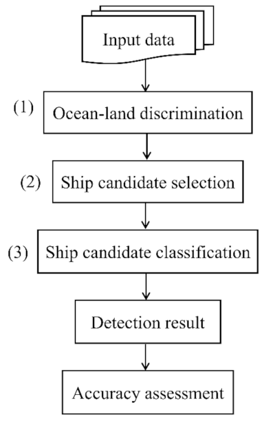
SD has a wide variety of environmental, civil, and military applications. For example, the benefits of automatic locating and tracking ships for the civil sector are maritime management, vessel traffic services, safety and rescue, fishery management, and illegal fishery surveillance. Moreover, the main applications in the military sector include naval warfare, battlefield environment assessment, and pirate activity surveillance [313,314,315]. RS has a leading role in SD and monitoring because of its several advantages, such as the availability of open-access multitemporal datasets and large area coverage.
Although various RS datasets have been used for SD (e.g., hyperspectral [316], TIR [317], and UAV [318] imagery), optical, SAR, and HF radar are the most common RS systems for SD [313]. Table 6 summarizes the main advantages and disadvantages of each of these systems for SD.
SD methods using spaceborne RS (i.e., optical and SAR) datasets generally have three main steps (see Figure 9): (1) ocean–land segmentation, (2) ship candidate extraction, and (3) classification of ship candidates [319,320,321]. Since the objective of the corresponding studies is to detect ships in oceans, the first step is separating ocean and land regions. This is usually performed using GIS layers of coastlines. However, with the end-to-end DL SD methods, this step is not necessary anymore. Most of the SD research studies have focused on the second and third steps by developing better features for ship description and False Alarm Rate (FAR) reduction. For example, in the second step, a simple shape analysis is performed to remove obvious FAR and extract Regions of Interest (ROI) that may contain potential ship candidates. In the third step, the ship candidates are classified into ship and nonship classes.
In the following three subsections, the most commonly used approaches for SD using optical, SAR, and HF radar data are discussed. However, it should be noted that more advanced ML methods, such as DL, have been recently employed for SD with high accuracies. For instance, among many object detection DL methods, the Region-based CNN (RCNN) [322] and its modified versions (e.g., Fast-RCNN [323] and Faster-RCNN [324]) are mostly used for SD. RCNN-based methods involve two major steps: (1) a CNN algorithm extracts the shared feature maps, and the region proposal network algorithm generates candidate regions, including potential ship targets; and (2) the network classifies these proposals into specified classes. DL methods can extract semantic-level features that are robust to varying ship sizes and different ocean conditions, resulting in better performance than traditional methods with human-crafted features and descriptors. However, the main limitation of DL methods is the limited accessibility to sufficient reference sample data [325,326].

3.6.1. Optical

With the advent of high-resolution optical systems, the volume of high spatiotemporal resolution imagery is growing, making them suitable for SD and monitoring applications [314]. Although optical RS systems can only operate during the daytime, recently, there has been a considerable focus on SD using optical imagery due to increasing the number of Very High Resolution (VHR) optical sensors [327]. There are a variety of methods for SD using optical images, such as threshold-based methods [328], anomaly detection [321], transform domain methods [313], Bayesian decision [329], shape and texture [314], and visual saliency [330]. In this study, the methods based on visual saliency and shape and texture are discussed in detail due to their relatively good performance and popularity.
A common approach for SD using optical images is applying the methods based on shape and texture features. These methods are robust and provide high accuracy in SD. However, false alarms (wakes and ocean clutter) still exist. So far, several studies have used the shape and texture features extracted from VHR optical satellite images for SD. For example, Zhu et al. [314] proposed an SD method based on shape and texture features using a combination of China–Brazil Earth Resources Satellite (CBERS) and SPOT images with a hierarchical coarse-to-fine FAR elimination process. They first carried out global and local image segmentation. Then, a simple shape analysis (e.g., region area and aspect ratio) was employed to remove obvious false candidates. Subsequently, finer shape features (e.g., compactness, rectangularity, and moment invariants), texture features (e.g., simple texture, wavelet-based, Multiscale Gaussian Differential Features (MGDFs)), and a novel operator, called local multiple pattern, proposed based on local binary pattern, were employed. Finally, they adopted a semisupervised hierarchical classification using SVM to identify ships.
Another popular approach in SD using optical satellite data is implementing methods based on visual saliency. Inspired by the human visual system, the visual saliency method tries to extract candidate regions that attract human eyes [330]. For example, Qi et al. [330] presented a method for extracting salient signals using a Phase spectrum of Fourier Transform (PFT). The binary saliency map was calculated through an adaptive segmentation. Then, the image was homogenized using a homogeneous filter to make it smooth. Finally, the Otsu segmentation method was applied to extract ship candidate regions. For discriminating ship targets, they developed a novel descriptor, called Ship Histogram of Oriented Gradient (S-HOG), based on the symmetrical shape of the ship. Their results on GaoFen-1 satellite images showed that the method was robust in detecting ships of various sizes in different ocean conditions.
As discussed, other than the abovementioned traditional methods, DL algorithms along with optical data have been recently used for SD. For instance, Zhang et al. [325] proposed a method based on Faster-RCNN to detect small ships and gather ships in offshore and inland water scenes to cover shortcomings of the traditional approaches of SD. They first classified the images into water and nonwater areas and created small ROIs that might contain ships using the SVM classifier. Then, the ROIs were ingested into an RCNN-based algorithm. They also modified the network architecture of the Faster-RCNN by combining multiresolution convolutional features and performing ROI pooling on a larger feature map. Their modified Faster-RCNN showed higher precision than various state-of-the-art SD methods, including the original Faster-RCNN.

3.6.2. SAR

SAR systems have also been extensively utilized for SD due to their operational ability in all weather conditions and all times [314]. However, compared to optical imagery, they contain a higher amount of noise. Consequently, it is difficult to detect small ships using SAR data. Moreover, there are relatively few SAR satellites compared to optical systems, causing challenges for real-time ship tracking and monitoring [314].
Numerous algorithms have been developed for SD using SAR images, including coherent target decomposition [331], polarimetric entropy [332], wavelet transforms [333], and generalized-likelihood ratio test [334]. However, the most-used method in this regard is the Constant FAR (CFAR) [335]. The CFAR algorithm searches for bright pixels in SAR images by comparing their grayscale value to the surrounding pixels. The most important step in the CFAR method is to design a distribution model for the background to specify an associated Probability Density Function (PDF). The Gaussian distribution, K-distribution, and Gamma PDFs have been widely used in this regard. Then, the Probability of False Alarm (PFA) for the threshold T is calculated by Equation (4).
P F A = 1 T f p d f x d x = T f p d f x d x
The conventional CFAR algorithm only considers the intensity value of the pixels. However, this can be due to the SAR ambiguities and ocean clutter in complex ocean conditions [320,321]. Therefore, FAR increases by incorrectly detecting bright clutter pixels as ships and missing some not-that-bright ship pixels due to factors such as speckles, incident angels, and materials of targets. With the advent of high spatial resolution SAR systems, such as TerraSAR-X and Sentinel-1, researchers are encouraged to take advantage of spatial relationships alongside the intensity of pixels to improve the conventional CFAR algorithm. For example, Leng et al. [336] proposed the bilateral CFAR algorithm, which used kernel density estimation as an analytical tool to determine the structure of the targets. Then, a combined value was generated using both intensity and spatial distributions. Finally, the standard CFAR method was applied to the SAR images with combined values to detect targets. Their results indicated that the bilateral CFAR reduced FAR compared to the conventional CFAR. Moreover, Wang et al. [337] proposed an Intensity-Space (IS) domain CFAR SD algorithm based on two factors [337]: (1) two neighboring pixels are more likely to be of the same kind, and (2) two pixels with similar intensity have a higher probability of belonging to the same class. In the IS-CFAR algorithm, intensity and locality were considered at the same time, as opposed to the sequential approach of the bilateral CFAR algorithm, and thus, the image was mapped into the IS domain to create a new transformed image. Then, the CFAR method was applied to extract ship targets. Finally, the results were refined using three target features of the target region area, form factor, and aspect ratio to further eliminate false alarms. The results showed that this method performed better than the bilateral CFAR only in terms of true target detection precision.
DL methods have also been widely investigated for SD using SAR data. For example, Jiao et al. [338] proposed an end-to-end, densely connected multiscale neural network based on Faster-RCNN for SD in SAR images [338]. They densely connected feature maps to each other from top to down, instead of using one feature map for region proposal, to achieve multiscale and multiscene (inshore and offshore) SD without ocean–land segmentation. They also proposed a training scheme to decrease the weight of easy-to-detect targets to decrease FAR in SD. Their results on multiresolution public SAR data, including imagery from RADARSAT-2, TerraSAR-X, Sentinel-1, and GaoFen-3, indicated the effectiveness of the method and its superiority over the Faster-RCNN algorithm. However, false alarms were observed, and the method had a problem when two ships were side by side (they were detected as one ship).

3.6.3. HF Radar

HF radars based on electromagnetic scattering and surface wave propagation can detect and track targets far beyond the conventional microwave radar coverage [339,340]. HF radars exploit the HF band (3–30 MHz) to offer a board coverage extended to more than 200 km in the range [340]. However, the radio frequency interferences and external noise restrict the detection capability of the HF radars [184,185]. Regarding SD using HF radar data, the sea clutter is considered to be self-generated interference and creates the first- and second-order resonant scattering effects in the Doppler spectrum. The first-order scattering is produced by ocean waves with half of the radar wavelength, while the second-order scattering is caused by the interaction of crossing sea waves [340]. SD using HF radar is mainly based on the CFAR algorithm following the beamforming data process. The CFAR threshold is usually calculated by the Neyman–Pearson approach and assuming a fixed PFA [341]. With this approach, a detection decision is made for each Range-Doppler (RD) cell.
Many studies have so far utilized HF radar data for SD. For example, in Dzvonkovskaya and Rohling [341], the adaptive threshold is obtained by applying the conventional curvilinear regression analysis [342] along with the Doppler and range cells to detect ships. Additionally, the gating approach was used to associate each target plot with a track in polar coordinates in order to track targets such as ships. Moreover, in Gorski et al. [343], target detection was accomplished by applying the space-time adaptive processing technique to each range cell. This algorithm was operated on a so-called data cube including complex samples, obtained from many coherent pulses for various range cells to acquire test statistics.
Although the aforementioned approaches are applicable for SD using HF radar, several issues may emerge when an HF radar observes the ocean surface and monitors moving ships. The first issue is that ships’ maneuvering during a long coherent processing interval creates Doppler blur in the Range-Doppler map. Therefore, SD may fail when the CFAR detector is applied. The second issue is that the Bragg scattering may mask a ship signal or be a considerable source of false detection since Range-Doppler cells associated with the Bragg scattering have a significant magnitude. In this regard, Roarty et al. [344] attempted to decrease the effect of ship maneuvers by applying a median filter before CFAR detection. Additionally, the decision fusion technique can be used for improving the detection performance to solve the second issue [70]. Park et al. [345] proposed a method to simultaneously solve the two abovementioned issues by adding a signal-enhancement procedure before CFAR detection. Finally, Hong et al. [346] proposed a DL method for SD using a combination of SAR and optical images. They developed a novel, robust framework based on a real-time object detection model, called YOLO, to improve the SD results compared to previous methods in the context of multisource, multiscale, and multisensor datasets. It was reported that their model could detect ships at any time with any available RS imagery with a high accuracy.

3.6.4. Summary and Future Direction

In summary, optical and SAR images have been extensively used for SD. However, they have usually been employed separately, and multisensor approaches have rarely been explored. Each of these data has its own advantages and disadvantages, and combining them for SD overcomes their limitations and provides better results. The focus of the future SD studies using SAR images should be concentrated on incorporating more precise spatial feature extraction and speeding up the algorithms of the spatial information extraction. This can improve the detection accuracy and reduce the detection time consumption [336]. Furthermore, in case of the existence of cooperative positioning data, more accurate and better results can be achieved.
DL methods have shown promising results for a variety of SAR applications. However, some further investigations are suggested for SD. First, more annotated SAR data are needed for accurate detection because it can improve the learning network. Thus, it is expected that more high-quality SAR datasets for SD will be provided for research in the future [338]. Additionally, it is recommended to concentrate on improving the segmentation algorithms in terms of both accuracy and computation time. In terms of optical images, it might be valuable to carry out more research on more complex CNN and RNN methods [325]. Moreover, regarding the spaceborne RS technology, it is worthwhile to exploit the hyperspectral data to for SD.

4. Conclusions

The pivotal role of oceans in regulating climate patterns, transportation, provision of human food, and economic growth is beyond any dispute. To this end, RS systems have been widely used to tackle the issues with the traditional in situ or shipborne approaches. In the first part of this review paper, 12 different RS systems, which are frequently utilized for ocean studies, and six oceanographic applications of RS systems (i.e., OSW, OSC, OWH, SL, OT, and SD) were discussed.
RS of OSW depends on the emissive and reflective properties of the ocean surface. Microwave radiometer, GNSS-R, SAR, scatterometers, and HF radar are the systems widely used for OSW estimation. Microwave radiometers provide large-scale coverage and are suitable for high wind speeds. However, they have coarse spatial resolution and suffer from low accuracy for estimating OSW direction in low wind speeds. Higher spatial and temporal resolutions and less sensitivity to atmospheric attenuation are the major privileges of GNSS-R systems for OSW estimation. SAR systems providing high spatial resolution are applicable at both low and high wind speeds. However, speckle noise issue and challenging preprocessing steps are the main drawbacks of SAR systems for OSW studies. Scatterometers provide acceptable efficiency in low wind speeds. They can be used for the entire globe at the cost of coarse spatial resolution. HF radars can provide appropriate accuracy at diverse wind speeds, but OSW data are only available at specific coastal regions where the HF radar has been installed.
There are many RS systems to directly/indirectly estimate OSC. Among these systems, HF and marine radar (i.e., X-band/C-band) provide a more accurate estimation of coastal OSC and its variations by real-time observations. However, they need costly maintenance and are not applicable for global OSC estimations. Therefore, the altimeter satellites have been commonly used to provide geostrophic OSC at a global scale with a high temporal frequency. However, the altimetry measurements are negatively affected by weather conditions and atmospheric variations and need corrections before being used in the OSC estimation.
Different RS systems, such as GNSS-R, SAR, altimeter, and marine radar, have been utilized for OWH estimation. GNSS-R systems have high temporal and spatial resolutions but have relatively low accuracy for OWH estimation. Although SAR data are less affected by the atmosphere, they are more affected by ocean surface substances. Altimeters also suffer from low spatial and temporal resolutions, as well as sensitivity to wind and wave directions. Although HF radars lack sufficient data availability, they provide accurate measurements of OWH and are operational in all-weather and day/night conditions. Marine radars provide a better SNR ratio and are cost-effective, but they can only be used for local scales.
Both active and passive RS systems can also measure SL and its variations. GNSS-R is often employed for global and regional SL monitoring. However, obtaining high accuracy in SL estimation with such systems requires long-term GNSS-R observations. Moreover, altimeters have been widely used for global SL mapping with a relatively coarse spatial resolution. Gravimetry satellites are used for measuring SL changes and distribution of ocean mass in very coarse spatial resolutions.
RS systems can be utilized to investigate various aspects of OT, such as tidal flats, tidal channels, tidal currents, OTL, and tidal wetlands. Optical, GNSS-R, SAR, altimeter, and LiDAR systems have been used for OT studies. Optical systems are not good at estimating water height changes but provide a wide range of spectral and spatial resolutions. The NRT data of GNSS-R are also important resources for OT studies. SAR systems are useful for all OT applications because they estimate ocean surface topographic changes with a high accuracy level. Altimeters benefit from multilook processing, but they are applicable only to tidal channels and tidal flats. Finally, LiDAR systems are useful for data acquisition at optimal tidal levels. Optical, SAR, and HF radar are the most commonly used RS systems for SD. Optical systems are only applicable in the daytime and are affected by clouds. Although SAR and HF radar are operational in all weather conditions and all times, the interpretation of the data acquired by the former system is difficult, and the latter system suffers from a lack of data availability.
Thanks to the high number of RS systems, along with their consistent archived datasets, the ocean RS experienced the big data era over the recent years. Big RS data in oceans provide the required datasets for advanced ML algorithms (e.g., DL). However, high performance, cloud computing platforms are required to efficiently process these big geo data. There is still plenty of room for future improvements in mapping various oceanographic parameters using DL models. For example, multidecade RS data series contain much hidden and critical information about oceans, which can be effectively investigated using advanced ML and cloud computing algorithms.

Author Contributions

M.A. designed and supervised the entire study, professionally optimized and revised all sections, and wrote the Abstract and Introduction sections; Section 2.1 was written by S.H.A.M. and S.A.A.; Section 2.2 was written by M.A., R.M.A., S.M.M., H.E., A.G., A.N., A.M. and S.O.; Section 3.1 was written by S.O., H.E. and M.E.N.; Section 3.2 was written by A.M.; Section 3.3 was written by S.O., A.N. and M.E.N.; Section 3.4 was written by A.G.; Section 3.5 was written by S.M.M.; Section 3.6 was written by B.R. and M.E.N.; Section 4 was written by S.M. (Soroosh Mehravar). All sections were professionally optimized and revised by F.M., S.M. (Sahel Mahdavi) and S.J. All authors have read and agreed to the published version of the manuscript..

Funding

This research received no external funding.

Institutional Review Board Statement

Not applicable.

Informed Consent Statement

Not applicable.

Conflicts of Interest

The authors declare no conflict of interest.

Appendix A

Table A1. Acronyms and corresponding descriptions.
AcronymDescription
ADDMVAllan Delay-Doppler Map Variance
AMSRAdvanced Microwave Scanning Radiometers
AODAtmospheric and Ocean De-aliasing
ASCATAdvanced SCATterometer
AT-InSARAlong-Track InSAR
AVHRRAdvanced Very High-Resolution Radiometer
AVISOArchiving, Validation, and Interpretation of Satellite Oceanographic
AWEIAutomated Water Extraction Index
BTBrightness Temperature
BTDBrightness Temperature Difference
BTDSFDifference between the temperature of sea surface and fog (BTSea surface − BTFog)
BTDTMBrightness Temperature Difference recorded by the Thermal Infrared and Mid Infrared bands (i.e., BTTIR − BTMIR)
CAACivil Aviation Authority
CBERSChina–Brazil Earth Resources Satellite
CEOFComplex Empirical Orthogonal Functions
CFARConstant FAR
CNNConvolutional Neural Network
CONUSContinental United States
CPICoherent Processing Interval
CSRCenter of Space Research
CTDCoherent Target Decomposition
CVIComposite Vulnerability Index
CYGNSSCyclone Global Navigation System Satellite
DCADoppler Centroid Anomaly
DDMADelay-Doppler Map Average
DDMsDelay-Doppler Maps
DDMVDelay-Doppler Map Variance
DEMDigital Elevation Model
DFODepartment of Fisheries and Oceans
DInSARDifferential InSAR
DLDeep Learning
DSMDigital Surface Model
ERSEuropean Remote Sensing
ESAEuropean Space Agency
ETSEquitable Threat Score
EVIEnhanced Vegetation Index
FARFalse Alarm Rate
GFZGeoForschungsZentrum
GNSSGlobal Navigation Satellite Systems Reflectometry
GNSS-RGNSS-Reflectometry
GNSS WGGNSS Wave Glider
GOES-16Geostationary Operational Environmental Satellite system-16
GLONASSGlobal Navigation Satellite System
GMFGeophysical Model Function
GMSLGlobal Mean SL
GPSGlobal Positioning System
GRACEGravity Recovery and Climate Experiment
GRDGround Range Detected
HFHigh Frequency
HFHSSWRHF Hybrid Sky–Surface Wave Radar
HRCHigh-Resolution Current
ICOADSInternational Comprehensive Ocean-Atmosphere Data Set
IFRInstrument Flight Rules
InIRAImaging Radar Altimeter
InSARInterferometric SAR
INSATIndian National Satellite
IPCCIntergovernmental Panel for Climate Change
IRNSSIndian Regional Navigation Satellite System
ISIntensity-Space
LBPLocal Binary Pattern
LEOLow Earth Orbit
LESLeading Edge Slope
LiDARLight Detection and Ranging
LIFRLow Instrument Flight Rules
LMPLocal Multiple Pattern
LOSLine of Sight
LSWILand Surface Water Index
LUTLook-Up Table
MANMARManual of Marine Weather Observations
MCCMaximum Cross-Correlation
METARMeteorological Aerodrome Report
MetOpMeteorological Operational satellite
MGDFsMultiscale Gaussian Differential Features
MIRMid Infrared
MLMachine Learning
MLE4Maximum Likelihood Estimator
MNDWIModified Normalized Difference Water Index
MSAVIModified Soil-Adjusted Vegetation Index
MVMinimum Variance
MVFRMarginal Visual Flight Rules
NAIPNational Agriculture Imagery Program
NASANational Aeronautics and Space Administration
NDBCNational Data Buoy Center
NDVINormalized Difference Vegetation Index
NDWINormalized Difference Water Index
NIRNear-Infrared
NLNewfoundland and Labrador
NOAANational Oceanic and Atmospheric Administration
NRCSNormalized Radar Cross Section
NRTNear Real-Time
NOAANational Oceanic and Atmospheric Administration
NSFNighttime Sea Fog
NWPNumerical Weather Prediction
OCOcean Color
OOSOcean Oil Spill
OSOcean Salinity
OSCOcean Surface Current
OSCAROcean Surface Current Analysis Real-time
OSWOcean Surface Wind
OTOcean Tide
OTLOcean Tidal Load
OTVOptimum Threshold Value
OWHOcean Wave Height
PDFProbability Density Function
PEPolarimetric Entropy
PFTPhase spectrum of Fourier Transform
PODProbability Of Detection
PPPPrecise Point Positioning
PRFPulse Repetition Frequency
P r S t d Probability of Nighttime Sea Fog for each pixel obtained from the spatial uniformity analysis
PrNSFProbability of Nighttime Sea Fog for each potential fog pixel
P r B T D T M Probability of Nighttime Sea Fog for each potential fog pixel obtained from the BTDTM
P r B T D S F Probability of Nighttime Sea Fog for each potential fog pixel obtained from the BTDSF
QuikSCATQuick SCATterometer
QZSSQuasi-Zenith Satellite System
RCNNRegion-based CNN
RDMRange-Doppler Map
RFRandom Forest
RIOPSRegional Ice-Ocean Prediction System
RMSERoot Mean Square Error
ROIRegions of Interest
RPNRegion Proposal Network
RSRemote Sensing
RSLRRelative SL Rise
RTRadiative Transfer
SARSynthetic Aperture Radar
SARALSatellite with ARgos and ALtiKa
SDShip Detection
SGR-ReSISpace GNSS Receiver Remote Sensing Instrument
S-HOGShip Histogram of Oriented Gradient
SHPSecond-order Harmonic Peaks
SISea Ice
SLSea Level
SLCSingle Look Complex
SMAPSoil Moisture Active Passive
SMVSignificant Minimum Value
SMOSSoil Moisture and Ocean Salinity
SNRSignal-to-Noise Ratio
SONARSound Navigation Ranging
SQGSurface Quasi-Geostrophic
SSTSea Surface Temperature
STAPSpace-Time Adaptive Processing
SVMSupport Vector Machine
SWIRShortwave Infrared
StdStandard deviation
TDS-1TechDemoSat-1
TESTrailing Edge Slope
TIRThermal Infrared
UAVUnmanned Aerial Vehicle
UK-DMCUnited Kingdom Disaster Monitoring Constellation
UTCUniversal Time Coordinated
VHRVery High Resolution
WaMoSWave and Current Analysis and Wave Spectra

References

  1. Devi, G.K.; Ganasri, B.P.; Dwarakish, G.S. Applications of Remote Sensing in Satellite Oceanography: A Review. Aquat. Procedia 2015, 4, 579–584. [Google Scholar] [CrossRef]
  2. Gholizadeh, M.H.; Melesse, A.M.; Reddi, L. A comprehensive review on water quality parameters estimation using remote sensing techniques. Sensors 2016, 16, 1298. [Google Scholar] [CrossRef] [Green Version]
  3. Bollmann, M. World ocean review: Living with the oceans. 2010. Available online: http://hdl.handle.net/1834/31403 (accessed on 12 December 2021).
  4. Amani, M.; Mahdavi, S.; Bullock, T.; Beale, S. Automatic nighttime sea fog detection using GOES-16 imagery. Atmos. Res. 2020, 238, 104712. [Google Scholar] [CrossRef]
  5. Honne Gowda, H.; Manikiam, B.; Jayaraman, V.; Chandrasekhar, M. Impact of satellite remote sensing on ocean modeling—An overview. Int. J. Remote Sens. 1993, 14, 3317–3331. [Google Scholar] [CrossRef]
  6. Minnett, P.; Alvera-Azcárate, A.; Chin, T.; Corlett, G.; Gentemann, C.; Karagali, I.; Li, X.; Marsouin, A.; Marullo, S.; Maturi, E. Half a century of satellite remote sensing of sea-surface temperature. Remote Sens. Environ. 2019, 233, 111366. [Google Scholar] [CrossRef]
  7. O’Carroll, A.G.; Armstrong, E.M.; Beggs, H.M.; Bouali, M.; Casey, K.S.; Corlett, G.K.; Dash, P.; Donlon, C.J.; Gentemann, C.L.; Høyer, J.L. Observational needs of sea surface temperature. Front. Mar. Sci. 2019, 6, 420. [Google Scholar] [CrossRef]
  8. Mahdavi, S.; Amani, M.; Bullock, T.; Beale, S. A probability-based daytime algorithm for sea fog detection using GOES-16 imagery. IEEE J. Sel. Top. Appl. Earth Obs. Remote Sens. 2020, 14, 1363–1373. [Google Scholar] [CrossRef]
  9. Kruk, R.; Fuller, M.C.; Komarov, A.S.; Isleifson, D.; Jeffrey, I. Proof of concept for sea ice stage of development classification using deep learning. Remote Sens. 2020, 12, 2486. [Google Scholar] [CrossRef]
  10. Chi, J.; Kim, H.-C. Prediction of arctic sea ice concentration using a fully data driven deep neural network. Remote Sens. 2017, 9, 1305. [Google Scholar] [CrossRef] [Green Version]
  11. Gao, Y.; Gao, F.; Dong, J.; Wang, S. Transferred deep learning for sea ice change detection from synthetic-aperture radar images. IEEE Geosci. Remote Sens. Lett. 2019, 16, 1655–1659. [Google Scholar] [CrossRef]
  12. Marmanis, D.; Datcu, M.; Esch, T.; Stilla, U. Deep learning earth observation classification using ImageNet pretrained networks. IEEE Geosci. Remote Sens. Lett. 2015, 13, 105–109. [Google Scholar] [CrossRef] [Green Version]
  13. Liu, H.; Guo, H.; Zhang, L. SVM-based sea ice classification using textural features and concentration from RADARSAT-2 dual-pol ScanSAR data. IEEE J. Sel. Top. Appl. Earth Obs. Remote Sens. 2014, 8, 1601–1613. [Google Scholar] [CrossRef]
  14. Su, H.; Wang, Y.; Xiao, J.; Yan, X.-H. Classification of MODIS images combining surface temperature and texture features using the Support Vector Machine method for estimation of the extent of sea ice in the frozen Bohai Bay, China. Int. J. Remote Sens. 2015, 36, 2734–2750. [Google Scholar] [CrossRef]
  15. Tempfli, K.; Huurneman, G.; Bakker, W.; Janssen, L.L.; Feringa, W.; Gieske, A.; Grabmaier, K.; Hecker, C.; Horn, J.; Kerle, N. Principles of Remote Sensing: An Introductory Textbook; International Institute for Geo-Information Science and Earth Observation: Enschede, The Netherlands, 2009. [Google Scholar]
  16. Raizer, V. Optical Remote Sensing of Ocean Hydrodynamics; CRC Press: Boca Raton, FL, USA, 2019. [Google Scholar]
  17. Parsons, S.; Amani, M.; Moghimi, A. Ocean colour mapping using remote sensing technology and an unsupervised machine learning algorithm. J. Ocean Technol. 2021, 16, 103–115. [Google Scholar]
  18. Sathyendranath, S. Remote Sensing of Ocean Colour in Coastal, and Other Optically-Complex, Waters; International Ocean Colour Coordinating Group (IOCCG): Dartmouth, NS, Canada, 2000. [Google Scholar]
  19. Embury, O.; Merchant, C.J.; Filipiak, M.J. A reprocessing for climate of sea surface temperature from the along-track scanning radiometers: Basis in radiative transfer. Remote Sens. Environ. 2012, 116, 32–46. [Google Scholar] [CrossRef]
  20. De Michele, M.; Leprince, S.; Thiébot, J.; Raucoules, D.; Binet, R. Direct measurement of ocean waves velocity field from a single SPOT-5 dataset. Remote Sens. Environ. 2012, 119, 266–271. [Google Scholar] [CrossRef]
  21. Amani, M.; Macdonald, C.; Mahdavi, S.; Gullage, M.; So, J. Aquatic vegetation mapping using machine learning algorithms and bathymetric lidar data: A case study from newfoundland, canada. J. Ocean Technol. 2021, 16, 76–94. [Google Scholar]
  22. Liu, S.; Chi, M.; Zou, Y.; Samat, A.; Benediktsson, J.A.; Plaza, A. Oil spill detection via multitemporal optical remote sensing images: A change detection perspective. IEEE Geosci. Remote Sens. Lett. 2017, 14, 324–328. [Google Scholar] [CrossRef]
  23. Seydi, S.T.; Hasanlou, M.; Amani, M.; Huang, W. Oil Spill Detection Based on Multiscale Multidimensional Residual CNN for Optical Remote Sensing Imagery. IEEE J. Sel. Top. Appl. Earth Obs. Remote Sens. 2021, 14, 10941–10952. [Google Scholar] [CrossRef]
  24. Bonnington, A.; Amani, M.; Ebrahimy, H. Oil Spill Detection Using Satellite Imagery. Adv. Environ. Eng. Res. 2021, 2, 1. [Google Scholar] [CrossRef]
  25. Kahle, A.B. A simple thermal model of the earth's surface for geologic mapping by remote sensing. J. Geophys. Res. 1977, 82, 1673–1680. [Google Scholar] [CrossRef]
  26. Klemas, V. Remote sensing techniques for studying coastal ecosystems: An overview. J. Coast. Res. 2011, 27, 2–17. [Google Scholar]
  27. Gentemann, C.L.; Donlon, C.J.; Stuart-Menteth, A.; Wentz, F.J. Diurnal signals in satellite sea surface temperature measurements. Geophys. Res. Lett. 2003, 30, 1140. [Google Scholar] [CrossRef]
  28. Lu, Y.; Zhan, W.; Hu, C. Detecting and quantifying oil slick thickness by thermal remote sensing: A ground-based experiment. Remote Sens. Environ. 2016, 181, 207–217. [Google Scholar] [CrossRef]
  29. Amlien, J. Remote sensing of snow with passive microwave radiometers—A review of current algorithms. Report 2008, 1019, 52. [Google Scholar]
  30. Woodhouse, I.H. Introduction to Microwave Remote Sensing; CRC Press: Boca Raton, FL, USA, 2017. [Google Scholar]
  31. Gaiser, P.W.; St Germain, K.M.; Twarog, E.M.; Poe, G.A.; Purdy, W.; Richardson, D.; Grossman, W.; Jones, W.L.; Spencer, D.; Golba, G. The WindSat spaceborne polarimetric microwave radiometer: Sensor description and early orbit performance. IEEE Trans. Geosci. Remote Sens. 2004, 42, 2347–2361. [Google Scholar] [CrossRef]
  32. Yueh, S.H.; Wilson, W.J.; Dinardo, S.J.; Hsiao, S.V. Polarimetric microwave wind radiometer model function and retrieval testing for WindSat. IEEE Trans. Geosci. Remote Sens. 2006, 44, 584–596. [Google Scholar] [CrossRef]
  33. Zavorotny, V.U.; Gleason, S.; Cardellach, E.; Camps, A. Tutorial on remote sensing using GNSS bistatic radar of opportunity. IEEE Geosci. Remote Sens. Mag. 2014, 2, 8–45. [Google Scholar] [CrossRef] [Green Version]
  34. Zavorotny, V.U.; Voronovich, A.G. Scattering of GPS signals from the ocean with wind remote sensing application. IEEE Trans. Geosci. Remote Sens. 2000, 38, 951–964. [Google Scholar] [CrossRef] [Green Version]
  35. Clarizia, M.P.; Ruf, C.S.; Jales, P.; Gommenginger, C. Spaceborne GNSS-R minimum variance wind speed estimator. IEEE Trans. Geosci. Remote Sens. 2014, 52, 6829–6843. [Google Scholar] [CrossRef]
  36. Garrison, J.L.; Komjathy, A.; Zavorotny, V.U.; Katzberg, S.J. Wind speed measurement using forward scattered GPS signals. IEEE Trans. Geosci. Remote Sens. 2002, 40, 50–65. [Google Scholar] [CrossRef] [Green Version]
  37. Gleason, S.; Hodgart, S.; Sun, Y.; Gommenginger, C.; Mackin, S.; Adjrad, M.; Unwin, M. Detection and processing of bistatically reflected GPS signals from low earth orbit for the purpose of ocean remote sensing. IEEE Trans. Geosci. Remote Sens. 2005, 43, 1229–1241. [Google Scholar] [CrossRef] [Green Version]
  38. Wiehl, M.; Legrésy, B. Potential of reflected GNSS signals for ice sheet remote sensing. Prog. Electromagn. Res. 2003, 40, 177–205. [Google Scholar] [CrossRef] [Green Version]
  39. Unwin, M.; Jales, P.; Tye, J.; Gommenginger, C.; Foti, G.; Rosello, J. Spaceborne GNSS-reflectometry on TechDemoSat-1: Early mission operations and exploitation. IEEE J. Sel. Top. Appl. Earth Obs. Remote Sens. 2016, 9, 4525–4539. [Google Scholar] [CrossRef]
  40. Ruf, C.S.; Chew, C.; Lang, T.; Morris, M.G.; Nave, K.; Ridley, A.; Balasubramaniam, R. A new paradigm in earth environmental monitoring with the cygnss small satellite constellation. Sci. Rep. 2018, 8, 8782. [Google Scholar] [CrossRef] [PubMed] [Green Version]
  41. Baghdadi, N.; Zribi, M. Microwave Remote Sensing of Land Surfaces: Techniques and Methods; Elsevier: Amsterdam, The Netherlands, 2016. [Google Scholar]
  42. Ulaby, F.; Long, D. Microwave Radar and Radiometric Remote Sensing; University of Michigan Press: Ann Arbor, MI, USA, 2014. [Google Scholar]
  43. Long, D.G. Polar applications of spaceborne scatterometers. IEEE J. Sel. Top. Appl. Earth Obs. Remote Sens. 2016, 10, 2307–2320. [Google Scholar] [CrossRef] [Green Version]
  44. Figa-Saldaña, J.; Wilson, J.J.; Attema, E.; Gelsthorpe, R.; Drinkwater, M.R.; Stoffelen, A. The advanced scatterometer (ASCAT) on the meteorological operational (MetOp) platform: A follow on for European wind scatterometers. Can. J. Remote Sens. 2002, 28, 404–412. [Google Scholar] [CrossRef]
  45. Dong, X.; Zhu, D.; Lin, W.; Liu, H.; Jiang, J. A Ku-band rotating fan-beam scatterometer: Design and performance simulations. In Proceedings of the 2010 IEEE International Geoscience and Remote Sensing Symposium, Honolulu, HI, USA, 25–30 July 2010; pp. 1081–1084. [Google Scholar]
  46. Lin, C.-C.; Rommen, B.; Wilson, J.J.W.; Impagnatiello, F.; Park, P.S. An analysis of a rotating, range-gated, fanbeam spaceborne scatterometer concept. IEEE Trans. Geosci. Remote Sens. 2000, 38, 2114–2121. [Google Scholar]
  47. Vu, P.L.; Frappart, F.; Darrozes, J.; Marieu, V.; Blarel, F.; Ramillien, G.; Bonnefond, P.; Birol, F. Multi-satellite altimeter validation along the French Atlantic coast in the southern bay of Biscay from ERS-2 to SARAL. Remote Sens. 2018, 10, 93. [Google Scholar] [CrossRef] [Green Version]
  48. Gómez-Enri, J.; Cipollini, P.; Gommenginger, C.; Martin-Puig, C.; Vignudelli, S.; Woodworth, P.; Benveniste, J.; Villares, P. COASTALT: Improving radar altimetry products in the oceanic coastal area. In Remote Sensing of the Ocean, Sea Ice, and Large Water Regions 2008; SPIE: Bellingham, WA, USA, 2008; pp. 132–141. [Google Scholar]
  49. Elachi, C.; Im, K.; Li, F.; Rodriguez, E. Global digital topography mapping with a synthetic aperture scanning radar altimeter. Int. J. Remote Sens. 1990, 11, 585–601. [Google Scholar] [CrossRef]
  50. Le Roy, Y.; Deschaux-Beaume, M.; Mavrocordatos, C.; Aguirre, M.; Heliere, F. SRAL SAR radar altimeter for sentinel-3 mission. In Proceedings of the 2007 IEEE International Geoscience and Remote Sensing Symposium, Barcelona, Spain, 23–28 July 2007; pp. 219–222. [Google Scholar]
  51. Wahle, C.M.; Dwight, D. Trueblood, National Ocean Service: What Is Eutrophication? Available online: https://oceanservice.noaa.gov/facts/eutrophication.html (accessed on 1 September 2021).
  52. Lowell, K.; Calder, B.; Lyons, A. Measuring shallow-water bathymetric signal strength in lidar point attribute data using machine learning. Int. J. Geogr. Inf. Sci. 2021, 35, 1592–1610. [Google Scholar] [CrossRef]
  53. Rogers, J.N.; Parrish, C.E.; Ward, L.G.; Burdick, D.M. Evaluation of field-measured vertical obscuration and full waveform lidar to assess salt marsh vegetation biophysical parameters. Remote Sens. Environ. 2015, 156, 264–275. [Google Scholar] [CrossRef]
  54. Massot-Campos, M.; Oliver-Codina, G. Optical sensors and methods for underwater 3D reconstruction. Sensors 2015, 15, 31525–31557. [Google Scholar] [CrossRef] [Green Version]
  55. Chen, J. Satellite gravimetry and mass transport in the earth system. Geod. Geodyn. 2019, 10, 402–415. [Google Scholar] [CrossRef]
  56. Besson, A. Weighing Earth, Tracking Water: Hydrological Applications of Data from GRACE Satellites. Doctoral Dissertation, Department of Geology and Geophysics, Yale University, New Haven, CT, USA, 2018. [Google Scholar]
  57. Ivins, E.R.; James, T.S.; Wahr, J.O.; Schrama, E.J.; Landerer, F.W.; Simon, K.M. Antarctic contribution to sea level rise observed by GRACE with improved GIA correction. J. Geophys. Res. Solid Earth 2013, 118, 3126–3141. [Google Scholar] [CrossRef]
  58. Peralta-Ferriz, C.; Morison, J.H.; Wallace, J.M.; Bonin, J.A.; Zhang, J. Arctic Ocean circulation patterns revealed by GRACE. J. Clim. 2014, 27, 1445–1468. [Google Scholar] [CrossRef] [Green Version]
  59. Johnson, G.C.; Chambers, D.P. Ocean bottom pressure seasonal cycles and decadal trends from GRACE Release-05: Ocean circulation implications. J. Geophys. Res. Ocean. 2013, 118, 4228–4240. [Google Scholar] [CrossRef]
  60. Schrama, E.J.; Wouters, B. Revisiting Greenland ice sheet mass loss observed by GRACE. J. Geophys. Res. Solid Earth 2011, 116. [Google Scholar] [CrossRef] [Green Version]
  61. Wouters, B.; Gardner, A.S.; Moholdt, G. Global glacier mass loss during the GRACE satellite mission (2002–2016). Front. Earth Sci. 2019, 7, 96. [Google Scholar] [CrossRef] [Green Version]
  62. Velicogna, I.; Wahr, J. Time-variable gravity observations of ice sheet mass balance: Precision and limitations of the GRACE satellite data. Geophys. Res. Lett. 2013, 40, 3055–3063. [Google Scholar] [CrossRef] [Green Version]
  63. Waite, A.D. Sonar for Practising Engineers; Wiley: Hoboken, NJ, USA, 2002. [Google Scholar]
  64. Hare, R.; Whittaker, C.; Clarke, J.; Beaudoin, J. Establishing a Multibeam Sonar Evaluation Test Bed near Sidney, British Columbia. In Proceedings of the 2012 Canadian Hydrographic Conference, Niagara Falls, Ontario, Canada, 15–17 May 2012. [Google Scholar]
  65. McConnell, J.A.; Weber, T.C.; Lauchle, G.C.; Gabrielson, T.B. Development of a high frequency underwater acoustic intensity probe. In Proceedings of the OCEANS'02 MTS/IEEE, Biloxi, MI, USA, 29-31 October 2002; pp. 1924–1929. [Google Scholar]
  66. Rubio, A.; Mader, J.; Corgnati, L.; Mantovani, C.; Griffa, A.; Novellino, A.; Quentin, C.; Wyatt, L.; Schulz-Stellenfleth, J.; Horstmann, J. HF radar activity in European coastal seas: Next steps toward a pan-European HF radar network. Front. Mar. Sci. 2017, 4, 8. [Google Scholar] [CrossRef] [Green Version]
  67. Paduan, J.D.; Washburn, L. High-frequency radar observations of ocean surface currents. Annu. Rev. Mar. Sci. 2013, 5, 115–136. [Google Scholar] [CrossRef] [PubMed] [Green Version]
  68. Lipa, B.; Barrick, D.; Alonso-Martirena, A.; Fernandes, M.; Ferrer, M.I.; Nyden, B. Brahan project high frequency radar ocean measurements: Currents, winds, waves and their interactions. Remote Sens. 2014, 6, 12094–12117. [Google Scholar] [CrossRef] [Green Version]
  69. Wyatt, L.; Thompson, S.; Burton, R. Evaluation of high frequency radar wave measurement. Coast. Eng. 1999, 37, 259–282. [Google Scholar] [CrossRef]
  70. Roarty, H.J.; Lemus, E.R.; Handel, E.; Glenn, S.M.; Barrick, D.E.; Isaacson, J. Performance evaluation of SeaSonde high-frequency radar for vessel detection. Mar. Technol. Soc. J. 2011, 45, 14–24. [Google Scholar] [CrossRef]
  71. Grilli, S.T.; Grosdidier, S.; Guérin, C.-A. Tsunami detection by high-frequency radar beyond the continental shelf. In Global Tsunami Science: Past and Future, Volume I; Springer: Berlin/Heidelberg, Germany, 2015; pp. 3895–3934. [Google Scholar]
  72. Chen, Z.; Zhang, B.; Kudryavtsev, V.; He, Y.; Chu, X. Estimation of sea surface current from X-band marine radar images by cross-spectrum analysis. Remote Sens. 2019, 11, 1031. [Google Scholar] [CrossRef] [Green Version]
  73. Hessner, K.; Reichert, K.; Borge, J.C.N.; Stevens, C.L.; Smith, M.J. High-resolution X-band radar measurements of currents, bathymetry and sea state in highly inhomogeneous coastal areas. Ocean Dyn. 2014, 64, 989–998. [Google Scholar] [CrossRef]
  74. Dankert, H.; Rosenthal, W. Ocean surface determination from X-band radar-image sequences. J. Geophys. Res. Ocean. 2004, 109, C04016. [Google Scholar] [CrossRef]
  75. Neill, S.P.; Hashemi, M.R. Fundamentals of Ocean Renewable Energy: Generating Electricity from the Sea; Academic Press: Cambridge, MA, USA, 2018. [Google Scholar]
  76. Chelton, D.B.; Schlax, M.G.; Freilich, M.H.; Milliff, R.F. Satellite measurements reveal persistent small-scale features in ocean winds. Science 2004, 303, 978–983. [Google Scholar] [CrossRef] [Green Version]
  77. Isaksen, L.; Stoffelen, A. ERS scatterometer wind data impact on ECMWF's tropical cyclone forecasts. IEEE Trans. Geosci. Remote Sens. 2000, 38, 1885–1892. [Google Scholar] [CrossRef]
  78. Rodríguez, E.; Bourassa, M.; Chelton, D.; Farrar, J.T.; Long, D.; Perkovic-Martin, D.; Samelson, R. The winds and currents mission concept. Front. Mar. Sci. 2019, 6, 438. [Google Scholar] [CrossRef]
  79. Villas Bôas, A.B.; Ardhuin, F.; Ayet, A.; Bourassa, M.A.; Brandt, P.; Chapron, B.; Cornuelle, B.D.; Farrar, J.T.; Fewings, M.R.; Fox-Kemper, B. Integrated observations of global surface winds, currents, and waves: Requirements and challenges for the next decade. Front. Mar. Sci. 2019, 6, 425. [Google Scholar] [CrossRef]
  80. Fang, H.; Xie, T.; Perrie, W.; Zhao, L.; Yang, J.; He, Y. Ocean wind and current retrievals based on satellite SAR measurements in conjunction with buoy and HF radar data. Remote Sens. 2017, 9, 1321. [Google Scholar] [CrossRef] [Green Version]
  81. Bourassa, M.; Stoffelen, A.; Bonekamp, H.; Chang, P.; Chelton, D.; Courtney, J.; Edson, R.; Figa, J.; He, Y.; Hersbach, H. Remotely sensed winds and wind stresses for marine forecasting and ocean modeling. Proc. Ocean. 2010, 9. [Google Scholar] [CrossRef] [Green Version]
  82. Hilburn, K.A.; Meissner, T.; Wentz, F.J.; Brown, S.T. Ocean vector winds from WindSat two-look polarimetric radiances. IEEE Trans. Geosci. Remote Sens. 2015, 54, 918–931. [Google Scholar] [CrossRef]
  83. Meissner, T.; Wentz, F.J. Wind-vector retrievals under rain with passive satellite microwave radiometers. IEEE Trans. Geosci. Remote Sens. 2009, 47, 3065–3083. [Google Scholar] [CrossRef]
  84. Ricciardulli, L.; Meissner, T.; Wentz, F. Towards a climate data record of satellite ocean vector winds. In Proceedings of the 2012 IEEE International Geoscience and Remote Sensing Symposium, Munich, Germany, 22–27 July 2012; pp. 2067–2069. [Google Scholar]
  85. Meissner, T.; Wentz, F. Ocean retrievals for WindSat: Radiative transfer model, algorithm, validation. In Proceedings of the OCEANS 2005 MTS/IEEE, Washington, DC, USA, 17–23 September 2005; pp. 130–133. [Google Scholar]
  86. Meissner, T.; Wentz, F.J.; Ricciardulli, L. The emission and scattering of L-band microwave radiation from rough ocean surfaces and wind speed measurements from the Aquarius sensor. J. Geophys. Res. Ocean. 2014, 119, 6499–6522. [Google Scholar] [CrossRef]
  87. Fore, A.G.; Yueh, S.H.; Tang, W.; Stiles, B.W.; Hayashi, A.K. Combined active/passive retrievals of ocean vector wind and sea surface salinity with SMAP. IEEE Trans. Geosci. Remote Sens. 2016, 54, 7396–7404. [Google Scholar] [CrossRef]
  88. Reul, N.; Tenerelli, J.; Chapron, B.; Vandemark, D.; Quilfen, Y.; Kerr, Y. SMOS satellite L-band radiometer: A new capability for ocean surface remote sensing in hurricanes. J. Geophys. Res. Ocean. 2012, 117, C02006. [Google Scholar] [CrossRef] [Green Version]
  89. Yin, X.; Wang, Z.; Song, Q.; Huang, Y.; Zhang, R. Estimate of ocean wind vectors inside tropical cyclones from polarimetric radiometer. IEEE J. Sel. Top. Appl. Earth Obs. Remote Sens. 2017, 10, 1701–1714. [Google Scholar] [CrossRef]
  90. Hwang, P.A.; Fan, Y. Low-frequency mean square slopes and dominant wave spectral properties: Toward tropical cyclone remote sensing. IEEE Trans. Geosci. Remote Sens. 2018, 56, 7359–7368. [Google Scholar] [CrossRef]
  91. Jales, P. Spaceborne Receiver Design for Scatterometric GNSS Reflectometry; University of Surrey: Guildford, UK, 2012. [Google Scholar]
  92. Foti, G.; Gommenginger, C.; Jales, P.; Unwin, M.; Shaw, A.; Robertson, C.; Rosello, J. Spaceborne GNSS reflectometry for ocean winds: First results from the UK TechDemoSat-1 mission. Geophys. Res. Lett. 2015, 42, 5435–5441. [Google Scholar] [CrossRef] [Green Version]
  93. Ruf, C.S.; Atlas, R.; Chang, P.S.; Clarizia, M.P.; Garrison, J.L.; Gleason, S.; Katzberg, S.J.; Jelenak, Z.; Johnson, J.T.; Majumdar, S.J. New ocean winds satellite mission to probe hurricanes and tropical convection. Bull. Am. Meteorol. Soc. 2016, 97, 385–395. [Google Scholar] [CrossRef]
  94. Bu, J.; Yu, K.; Zhu, Y.; Qian, N.; Chang, J. Developing and testing models for sea surface wind speed estimation with GNSS-R delay doppler maps and delay waveforms. Remote Sens. 2020, 12, 3760. [Google Scholar] [CrossRef]
  95. Ruf, C.S.; Balasubramaniam, R. Development of the CYGNSS geophysical model function for wind speed. IEEE J. Sel. Top. Appl. Earth Obs. Remote Sens. 2018, 12, 66–77. [Google Scholar] [CrossRef]
  96. Yang, X.; Li, X.; Pichel, W.G.; Li, Z. Comparison of ocean surface winds from ENVISAT ASAR, MetOp ASCAT scatterometer, buoy measurements, and NOGAPS model. IEEE Trans. Geosci. Remote Sens. 2011, 49, 4743–4750. [Google Scholar] [CrossRef]
  97. Beal, R.C. High Resolution wind Monitoring with Wide Swath SAR: A User's Guide; US Department of Commerce, National Oceanic and Atmospheric Administration: Silver Spring, MD, USA, 2005. [Google Scholar]
  98. Zhang, B.; Perrie, W. Cross-polarized synthetic aperture radar: A new potential measurement technique for hurricanes. Bull. Am. Meteorol. Soc. 2012, 93, 531–541. [Google Scholar] [CrossRef] [Green Version]
  99. Hwang, P.A.; Stoffelen, A.; van Zadelhoff, G.J.; Perrie, W.; Zhang, B.; Li, H.; Shen, H. Cross-polarization geophysical model function for C-band radar backscattering from the ocean surface and wind speed retrieval. J. Geophys. Res. Ocean. 2015, 120, 893–909. [Google Scholar] [CrossRef]
  100. Li, X.; Zhang, J.A.; Yang, X.; Pichel, W.G.; DeMaria, M.; Long, D.; Li, Z. Tropical cyclone morphology from spaceborne synthetic aperture radar. Bull. Am. Meteorol. Soc. 2013, 94, 215–230. [Google Scholar] [CrossRef] [Green Version]
  101. Wentz, F.J.; Ricciardulli, L.; Rodriguez, E.; Stiles, B.W.; Bourassa, M.A.; Long, D.G.; Hoffman, R.N.; Stoffelen, A.; Verhoef, A.; O'Neill, L.W. Evaluating and extending the ocean wind climate data record. IEEE J. Sel. Top. Appl. Earth Obs. Remote Sens. 2017, 10, 2165–2185. [Google Scholar] [CrossRef] [Green Version]
  102. Lin, C.-C.; Lengert, W.; Attema, E. Three generations of C-band wind scatterometer systems from ERS-1/2 to MetOp/ASCAT, and MetOp second generation. IEEE J. Sel. Top. Appl. Earth Obs. Remote Sens. 2016, 10, 2098–2122. [Google Scholar] [CrossRef]
  103. Guo, Q.; Xu, X.; Zhang, K.; Li, Z.; Huang, W.; Mansaray, L.R.; Liu, W.; Wang, X.; Gao, J.; Huang, J. Assessing global ocean wind energy resources using multiple satellite data. Remote Sens. 2018, 10, 100. [Google Scholar] [CrossRef] [Green Version]
  104. Sapp, J.W.; Alsweiss, S.O.; Jelenak, Z.; Chang, P.S.; Frasier, S.J.; Carswell, J. Airborne co-polarization and cross-polarization observations of the ocean-surface NRCS at C-band. IEEE Trans. Geosci. Remote Sens. 2016, 54, 5975–5992. [Google Scholar] [CrossRef]
  105. Stewart, R.H.; Barnum, J.R. Radio measurements of oceanic winds at long ranges: An evaluation. Radio Sci. 1975, 10, 853–857. [Google Scholar] [CrossRef]
  106. Maresca, J.; Barnum, J. Measurement of oceanic wind speed from HF sea scatter by skywave radar. IEEE Trans. Antennas Propag. 1977, 25, 132–136. [Google Scholar] [CrossRef]
  107. Barrick, D. Remote sensing of sea state by radar. In Proceedings of the Ocean 72-IEEE International Conference on Engineering in the Ocean Environment, Newport, RI, USA, 13–15 September 1972; pp. 186–192. [Google Scholar]
  108. Barrick, D.E.; Headrick, J.M.; Bogle, R.W.; Crombie, D.D. Sea backscatter at HF: Interpretation and utilization of the echo. Proc. IEEE 1974, 62, 673–680. [Google Scholar] [CrossRef]
  109. Ahearn, J.L.; Curley, S.R.; Headrick, J.M.; Trizna, D. Tests of remote skywave measurement of ocean surface conditions. Proc. IEEE 1974, 62, 681–687. [Google Scholar] [CrossRef]
  110. Dexter, P.; Theodoridis, S. Surface wind speed extraction from HF sky wave radar Doppler spectra. Radio Sci. 1982, 17, 643–652. [Google Scholar] [CrossRef]
  111. Huang, W.; Wu, S.; Gill, E.; Wen, B.; Hou, J. HF radar wave and wind measurement over the Eastern China Sea. IEEE Trans. Geosci. Remote Sens. 2002, 40, 1950–1955. [Google Scholar] [CrossRef]
  112. Klemas, V. Remote sensing of coastal and ocean currents: An overview. J. Coast. Res. 2012, 28, 576–586. [Google Scholar]
  113. Fu, L.-L.; Lee, T.; Liu, W.T.; Kwok, R. 50 years of satellite remote sensing of the ocean. Meteorol. Monogr. 2019, 59, 5.1–5.46. [Google Scholar] [CrossRef]
  114. Dohan, K.; Maximenko, N. Monitoring ocean currents with satellite sensors. Oceanography 2010, 23, 94–103. [Google Scholar] [CrossRef] [Green Version]
  115. Briney, A. How Ocean Currents Work. Available online: https://www.thoughtco.com/ocean-currents-1435343.2019 (accessed on 5 February 2021).
  116. Isern-Fontanet, J.; Ballabrera-Poy, J.; Turiel, A.; García-Ladona, E. Remote sensing of ocean surface currents: A review of what is being observed and what is being assimilated. Nonlinear Process. Geophys. 2017, 24, 613–643. [Google Scholar] [CrossRef] [Green Version]
  117. Gille, S.T.; Metzger, E.J.; Tokmakian, R. Seafloor Topography and Ocean Circulation; Naval Research Lab Stennis Space Center Ms Oceanography Div: Stennis Space Center, MS, USA, 2004. [Google Scholar]
  118. Dagestad, K.-F.; Röhrs, J. Prediction of ocean surface trajectories using satellite derived vs. modeled ocean currents modeled ocean currents. Remote Sens. Environ. 2019, 223, 130–142. [Google Scholar] [CrossRef]
  119. Ribbe, J.; Brieva, D. A western boundary current eddy characterisation study. Estuar. Coast. Shelf Sci. 2016, 183, 203–212. [Google Scholar] [CrossRef] [Green Version]
  120. Hartmann, D.L. Global Physical Climatology, 2nd ed.; Elsevier: Amsterdam, The Netherlands.
  121. Lazier, J.R.; Wright, D.G. Annual velocity variations in the Labrador Current. J. Phys. Oceanogr. 1993, 23, 659–678. [Google Scholar] [CrossRef]
  122. Joseph, A. Measuring Ocean Currents: Tools, Technologies, and Data, 1st ed.; Elsevier: Waltham, MA, USA.
  123. Constantin, A. Frictional effects in wind-driven ocean currents. Geophys. Astrophys. Fluid Dyn. 2021, 115, 1–14. [Google Scholar] [CrossRef] [Green Version]
  124. Pinet, P.R. Invitation to Oceanography; Jones & Bartlett Learning: Burlington, MA, USA, 2019. [Google Scholar]
  125. Rahmstorf, S. Thermohaline circulation: The current climate. Nature 2003, 421, 699. [Google Scholar] [CrossRef]
  126. Schott, F.A.; Zantopp, R.; Stramma, L.; Dengler, M.; Fischer, J.; Wibaux, M. Circulation and deep-water export at the western exit of the subpolar North Atlantic. J. Phys. Oceanogr. 2004, 34, 817–843. [Google Scholar] [CrossRef]
  127. Yurovskaya, M.; Kudryavtsev, V.; Chapron, B.; Collard, F. Ocean surface current retrieval from space: The Sentinel-2 multispectral capabilities. Remote Sens. Environ. 2019, 234, 111468. [Google Scholar] [CrossRef]
  128. Sun, H.; Song, Q.; Shao, R.; Schlicke, T. Estimation of sea surface currents based on ocean colour remote-sensing image analysis. Int. J. Remote Sens. 2016, 37, 5105–5121. [Google Scholar] [CrossRef]
  129. Carvajal, G.K.; Eriksson, L.E.; Ulander, L.M.; Berg, A. Comparison between current fields detected with infrared radiometry and modeled currents around Sweden. In Proceedings of the 2013 IEEE International Geoscience and Remote Sensing Symposium-IGARSS, Melbourne, VIC, Australia, 21–26 July 2013; pp. 1270–1273. [Google Scholar]
  130. Heuzé, C.; Carvajal, G.K.; Eriksson, L.E.; Soja-Woźniak, M. Sea surface currents estimated from spaceborne infrared images validated against reanalysis data and drifters in the Mediterranean Sea. Remote Sens. 2017, 9, 422. [Google Scholar] [CrossRef] [Green Version]
  131. Crocker, R.I.; Matthews, D.K.; Emery, W.J.; Baldwin, D.G. Computing coastal ocean surface currents from infrared and ocean color satellite imagery. IEEE Trans. Geosci. Remote Sens. 2007, 45, 435–447. [Google Scholar] [CrossRef]
  132. González-Haro, C.; Isern-Fontanet, J. Ocean surface currents reconstruction at a global scale from microwave measurements. In Proceedings of the 2012 IEEE International Geoscience and Remote Sensing Symposium, Munich, Germany, 22–27 July 2012; pp. 3780–3783. [Google Scholar]
  133. González-Haro, C.; Isern-Fontanet, J. Assessment of ocean surface currents reconstruction at a global scale from the synergy between microwave and altimetric measurements. In Proceedings of the 2013 IEEE International Geoscience and Remote Sensing Symposium-IGARSS, Melbourne, VIC, Australia, 21–26 July 2013; pp. 2950–2953. [Google Scholar]
  134. González-Haro, C.; Isern-Fontanet, J. Global ocean current reconstruction from altimetric and microwave SST measurements. J. Geophys. Res. Ocean. 2014, 119, 3378–3391. [Google Scholar] [CrossRef]
  135. González-Haro, C.; Isern-Fontanet, J.; Tandeo, P.; Garello, R. Ocean surface currents reconstruction: Spectral characterization of the transfer function between SST and SSH. J. Geophys. Res. Ocean. 2020, 125, e2019JC015958. [Google Scholar] [CrossRef]
  136. Elyouncha, A. Sea Surface Current Measurements Using Along-Track Interferometric SAR. Ph.D. Thesis, Chalmers Tekniska Hogskola (Sweden), Göteborg, Sweden, 2018. [Google Scholar]
  137. Lyzenga, D.R.; Marmorino, G.O. Measurement of surface currents using sequential synthetic aperture radar images of slick patterns near the edge of the Gulf Stream. J. Geophys. Res. Ocean. 1998, 103, 18769–18777. [Google Scholar] [CrossRef]
  138. Hansen, M.W.; Collard, F.; Dagestad, K.-F.; Johannessen, J.A.; Fabry, P.; Chapron, B. Retrieval of sea surface range velocities from Envisat ASAR Doppler centroid measurements. IEEE Trans. Geosci. Remote Sens. 2011, 49, 3582–3592. [Google Scholar] [CrossRef]
  139. Marghany, M.; Hashim, M. Robust of doppler centroid for mapping sea surface current by using radar satellite data. Am. J. Eng. Appl. Sci. 2009, 2, 781–788. [Google Scholar] [CrossRef]
  140. Fu, B.; Huang, W.; Fan, K.; Gan, X.; Zhang, H.; Shi, A. Method for ocean surface currents measurement by SAR. In Remote Sensing and Modeling of the Atmosphere, Oceans, and Interactions II; SPIE: Bellingham, WA, USA, 2008; Volume 7148, pp. 56–61. [Google Scholar]
  141. Elyouncha, A.; Eriksson, L.E.; Johnsen, H.; Ulander, L.M. Using Sentinel-1 ocean data for mapping sea surface currents along the southern Norwegian coast. In Proceedings of the IGARSS 2019-2019 IEEE International Geoscience and Remote Sensing Symposium, Yokohama, Japan, 28 July–2 August 2019; pp. 8058–8061. [Google Scholar]
  142. Townsend, W.; McGoogan, J.; Walsh, E. Satellite radar altimeters-present and future oceanographic capabilities. In Oceanography from Space; Springer: Berlin/Heidelberg, Germany, 1981; pp. 625–636. [Google Scholar]
  143. Roarty, H.; Cook, T.; Hazard, L.; George, D.; Harlan, J.; Cosoli, S.; Wyatt, L.; Alvarez Fanjul, E.; Terrill, E.; Otero, M. The global high frequency radar network. Front. Mar. Sci. 2019, 6, 164. [Google Scholar] [CrossRef]
  144. Mantovani, C.; Corgnati, L.; Horstmann, J.; Rubio, A.; Reyes, E.; Quentin, C.; Cosoli, S.; Asensio, J.L.; Mader, J.; Griffa, A. Best practices on high frequency radar deployment and operation for ocean current measurement. Front. Mar. Sci. 2020, 7, 210. [Google Scholar] [CrossRef] [Green Version]
  145. Ji, Y.; Zhang, J.; Chu, X.; Wang, Y.; Yang, L. Ocean surface current measurement with high-frequency hybrid sky–surface wave radar. Remote Sens. Lett. 2017, 8, 617–626. [Google Scholar] [CrossRef]
  146. Kolukula, S.S.; Baduru, B.; Murty, P.; Kumar, J.P.; Rao, E.; Shenoi, S. Gaps Filling in HF Radar Sea Surface Current Data Using Complex Empirical Orthogonal Functions. Pure Appl. Geophys. 2020, 177, 5969–5992. [Google Scholar] [CrossRef]
  147. Huang, W.; Wu, X.; Lund, B.; El-Darymli, K. Advances in coastal HF and microwave (S-or X-band) radars. Int. J. Antennas Propag. 2017, 2017, 3089046. [Google Scholar] [CrossRef] [Green Version]
  148. Cheng, H.-Y.; Chien, H. Implementation of S-band marine radar for surface wave measurement under precipitation. Remote Sens. Environ. 2017, 188, 85–94. [Google Scholar] [CrossRef]
  149. Neill, S.P.; Hashemi, M.R. Ocean modelling for resource characterization. Fundam. Ocean Renew. Energy 2018, 193–235. [Google Scholar] [CrossRef]
  150. Horstmann, J.; Carrasco, R.; Seemann, J.; Cysewski, M. Surface current measurements using marine radars. In Proceedings of the 2015 IEEE/OES Eleveth Current, Waves and Turbulence Measurement (CWTM), St. Petersburg, FL, USA, 2-6 March 2015; pp. 1–3. [Google Scholar]
  151. Hongo, C.; Kawamata, H.; Goto, K. Catastrophic impact of typhoon waves on coral communities in the Ryukyu Islands under global warming. J. Geophys. Res. Biogeosci. 2012, 117, G02029. [Google Scholar] [CrossRef]
  152. Osadchiev, A. Small mountainous rivers generate high-frequency internal waves in coastal ocean. Sci. Rep. 2018, 8, 16609. [Google Scholar] [CrossRef] [Green Version]
  153. Dobson, E.; Monaldo, F.; Goldhirsh, J.; Wilkerson, J. Validation of Geosat altimeter-derived wind speeds and significant wave heights using buoy data. J. Geophys. Res. Ocean. 1987, 92, 10719–10731. [Google Scholar] [CrossRef]
  154. Chowdhary, J.; Zhai, P.-W.; Boss, E.; Dierssen, H.; Frouin, R.; Ibrahim, A.; Lee, Z.; Remer, L.A.; Twardowski, M.; Xu, F. Modeling atmosphere-ocean radiative transfer: A PACE mission perspective. Front. Earth Sci. 2019, 7, 100. [Google Scholar] [CrossRef]
  155. Gabarró, C.; Font, J.; Camps, A.; Vall-llossera, M.; Julià, A. A new empirical model of sea surface microwave emissivity for salinity remote sensing. Geophys. Res. Lett. 2004, 31, L01309. [Google Scholar] [CrossRef] [Green Version]
  156. James, S.C.; Zhang, Y.; O'Donncha, F. A machine learning framework to forecast wave conditions. Coast. Eng. 2018, 137, 1–10. [Google Scholar] [CrossRef] [Green Version]
  157. Shao, Q.; Li, W.; Han, G.; Hou, G.; Liu, S.; Gong, Y.; Qu, P. A Deep Learning Model for Forecasting Sea Surface Height Anomalies and Temperatures in the South China Sea. J. Geophys. Res. Ocean. 2021, 126, e2021JC017515. [Google Scholar] [CrossRef]
  158. Liu, J.; Jin, B.; Wang, L.; Xu, L. Sea surface height prediction with deep learning based on attention mechanism. IEEE Geosci. Remote Sens. Lett. 2020, 19, 1501605. [Google Scholar] [CrossRef]
  159. Rius, A.; Cardellach, E.; Martin-Neira, M. Altimetric analysis of the sea-surface GPS-reflected signals. IEEE Trans. Geosci. Remote Sens. 2010, 48, 2119–2127. [Google Scholar] [CrossRef]
  160. Chen, F.; Liu, L.; Guo, F. Sea surface height estimation with multi-GNSS and wavelet de-noising. Sci. Rep. 2019, 9, 15181. [Google Scholar] [CrossRef] [Green Version]
  161. Larson, K.M.; Löfgren, J.S.; Haas, R. Coastal sea level measurements using a single geodetic GPS receiver. Adv. Space Res. 2013, 51, 1301–1310. [Google Scholar] [CrossRef]
  162. Santamaría-Gómez, A.; Watson, C.; Gravelle, M.; King, M.; Wöppelmann, G. Levelling co-located GNSS and tide gauge stations using GNSS reflectometry. J. Geod. 2015, 89, 241–258. [Google Scholar] [CrossRef]
  163. Penna, N.T.; Morales Maqueda, M.A.; Martin, I.; Guo, J.; Foden, P.R. Sea surface height measurement using a GNSS Wave Glider. Geophys. Res. Lett. 2018, 45, 5609–5616. [Google Scholar] [CrossRef]
  164. Zhang, B.; Perrie, W.; He, Y. Remote sensing of ocean waves by along-track interferometric synthetic aperture radar. J. Geophys. Res. Ocean. 2009, 114, C10015. [Google Scholar] [CrossRef] [Green Version]
  165. Lin, B.; Shao, W.; Li, X.; Li, H.; Du, X.; Ji, Q.; Cai, L. Development and validation of an ocean wave retrieval algorithm for VV-polarization Sentinel-1 SAR data. Acta Oceanol. Sin. 2017, 36, 95–101. [Google Scholar] [CrossRef]
  166. Shao, W.; Hu, Y.; Yang, J.; Nunziata, F.; Sun, J.; Li, H.; Zuo, J. An empirical algorithm to retrieve significant wave height from Sentinel-1 synthetic aperture radar imagery collected under cyclonic conditions. Remote Sens. 2018, 10, 1367. [Google Scholar] [CrossRef] [Green Version]
  167. Alpers, W.R.; Ross, D.B.; Rufenach, C.L. On the detectability of ocean surface waves by real and synthetic aperture radar. J. Geophys. Res. Ocean. 1981, 86, 6481–6498. [Google Scholar] [CrossRef]
  168. Mastenbroek, C.; De Valk, C. A semiparametric algorithm to retrieve ocean wave spectra from synthetic aperture radar. J. Geophys. Res. Ocean. 2000, 105, 3497–3516. [Google Scholar] [CrossRef]
  169. Jian, S.; Changlong, G. Parameterized first-guess spectrum method for retrieving directional spectrum of swell-dominated waves and huge waves from SAR images. Chin. J. Oceanol. Limnol. 2006, 24, 12–20. [Google Scholar] [CrossRef]
  170. Schulz-Stellenfleth, J.; Lehner, S.; Hoja, D. A parametric scheme for the retrieval of two-dimensional ocean wave spectra from synthetic aperture radar look cross spectra. J. Geophys. Res. Ocean. 2005, 110, C05004. [Google Scholar] [CrossRef] [Green Version]
  171. Wang, H.; Wang, J.; Yang, J.; Ren, L.; Zhu, J.; Yuan, X.; Xie, C. Empirical algorithm for significant wave height retrieval from wave mode data provided by the Chinese satellite Gaofen-3. Remote Sens. 2018, 10, 363. [Google Scholar] [CrossRef]
  172. Schulz-Stellenfleth, J.; König, T.; Lehner, S. An empirical approach for the retrieval of integral ocean wave parameters from synthetic aperture radar data. J. Geophys. Res. Ocean. 2007, 112, C03019. [Google Scholar] [CrossRef]
  173. Li, X.-M.; Lehner, S.; Bruns, T. Ocean wave integral parameter measurements using Envisat ASAR wave mode data. IEEE Trans. Geosci. Remote Sens. 2010, 49, 155–174. [Google Scholar] [CrossRef] [Green Version]
  174. Stopa, J.E.; Mouche, A. Significant wave heights from S entinel-1 SAR: Validation and applications. J. Geophys. Res. Ocean. 2017, 122, 1827–1848. [Google Scholar] [CrossRef] [Green Version]
  175. Bruck, M.; Lehner, S. TerraSAR-X/TanDEM-X sea state measurements using the XWAVE algorithm. Int. J. Remote Sens. 2015, 36, 3890–3912. [Google Scholar] [CrossRef]
  176. Shao, W.; Zhang, Z.; Li, X.; Li, H. Ocean wave parameters retrieval from Sentinel-1 SAR imagery. Remote Sens. 2016, 8, 707. [Google Scholar] [CrossRef] [Green Version]
  177. Tarpanelli, A.; Benveniste, J. On the potential of altimetry and optical sensors for monitoring and forecasting river discharge and extreme flood events. In Extreme Hydroclimatic Events and Multivariate Hazards in a Changing Environment; Elsevier: Amsterdam, The Netherlands, 2019; pp. 267–287. [Google Scholar]
  178. Wang, J.; Aouf, L.; Jia, Y.; Zhang, Y. Validation and calibration of significant wave height and wind speed retrievals from HY2B altimeter based on Deep Learning. Remote Sens. 2020, 12, 2858. [Google Scholar] [CrossRef]
  179. Peng, F.; Deng, X. Validation of improved significant wave heights from the Brown-Peaky (BP) retracker along the east coast of Australia. Remote Sens. 2018, 10, 1072. [Google Scholar] [CrossRef] [Green Version]
  180. Barrick, D.E. Extraction of wave parameters from measured HF radar sea-echo Doppler spectra. Radio Sci. 1977, 12, 415–424. [Google Scholar] [CrossRef]
  181. Gurgel, K.-W.; Essen, H.-H.; Schlick, T. An empirical method to derive ocean waves from second-order Bragg scattering: Prospects and limitations. IEEE J. Ocean. Eng. 2006, 31, 804–811. [Google Scholar] [CrossRef]
  182. Tian, Z.; Tian, Y.; Wen, B.; Wang, S.; Zhao, J.; Huang, W.; Gill, E.W. Wave-height mapping from second-order harmonic peaks of wide-beam HF radar backscatter spectra. IEEE Trans. Geosci. Remote Sens. 2019, 58, 925–937. [Google Scholar] [CrossRef]
  183. Zhou, H.; Wen, B. Radio frequency interference suppression in small-aperture high-frequency radars. IEEE Geosci. Remote Sens. Lett. 2012, 9, 788–792. [Google Scholar] [CrossRef]
  184. Nazari, M.E.; Huang, W.; Zhao, C. Dense Radio Frequency Interference Cancellation by CEMD and Temporal Windowing Processing for HFSW Radar. In Proceedings of the OCEANS 2019-Marseille, Marseille, France, 17–20 June 2019; pp. 1–4. [Google Scholar]
  185. Nazari, M.E.; Huang, W.; Zhao, C. Radio frequency interference suppression for HF surface wave radar using CEMD and temporal windowing methods. IEEE Geosci. Remote Sens. Lett. 2019, 17, 212–216. [Google Scholar] [CrossRef]
  186. Zhou, H.; Wen, B. Wave height extraction from the first-order Bragg peaks in high-frequency radars. IEEE Geosci. Remote Sens. Lett. 2015, 12, 2296–2300. [Google Scholar] [CrossRef]
  187. Tian, Y.; Wen, B.; Zhou, H.; Wang, C.; Yang, J.; Huang, W. Wave height estimation from first-order backscatter of a dual-frequency high frequency radar. Remote Sens. 2017, 9, 1186. [Google Scholar] [CrossRef] [Green Version]
  188. Huang, W.; Liu, X.; Gill, E.W. Ocean wind and wave measurements using X-band marine radar: A comprehensive review. Remote Sens. 2017, 9, 1261. [Google Scholar] [CrossRef] [Green Version]
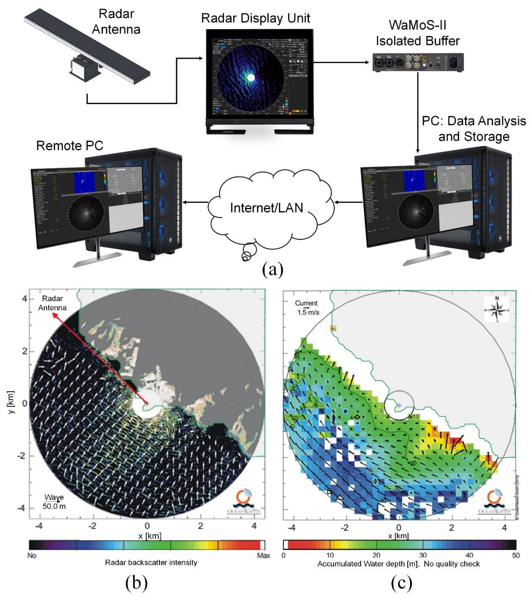
  189. Hessner, K.G.; Nieto-Borge, J.C.; Bell, P.S. Nautical radar measurements in Europe: Applications of WaMoS II as a sensor for sea state, current and bathymetry. In Remote Sensing of the European Seas; Springer: Berlin/Heidelberg, Germany, 2008; pp. 435–446. [Google Scholar]
  190. Vicen-Bueno, R.; Lido-Muela, C.; Nieto-Borge, J.C. Estimate of significant wave height from non-coherent marine radar images by multilayer perceptrons. EURASIP J. Adv. Signal Process. 2012, 2012, 84. [Google Scholar] [CrossRef] [Green Version]
  191. Chuang, L.Z.-H.; Wu, L.-C.; Doong, D.-J.; Kao, C.C. Two-dimensional continuous wavelet transform of simulated spatial images of waves on a slowly varying topography. Ocean Eng. 2008, 35, 1039–1051. [Google Scholar] [CrossRef]
  192. Ma, K.; Wu, X.; Yue, X.; Wang, L.; Liu, J. Array beamforming algorithm for estimating waves and currents from marine X-band radar image sequences. IEEE Trans. Geosci. Remote Sens. 2016, 55, 1262–1272. [Google Scholar] [CrossRef]
  193. Henschel, M.; Buckley, J.; Dobson, F. Estimates of wave height from low incidence angle sea clutter. Proceedings of the Fourth International Workshop on Wave Hindcasting and Forecasting; Federal Panel on Energy R&D, 1995. Available online: https://www.google.com.hk/url?sa=t&rct=j&q=&esrc=s&source=web&cd=&cad=rja&uact=8&ved=2ahUKEwjqjtDjrf36AhXH9zgGHeDdC2EQFnoECAgQAQ&url=https%3A%2F%2Fwaves-vagues.dfo-mpo.gc.ca%2FLibrary%2F223549.pdf&usg=AOvVaw393d9o6YAGnWxW6h4MfTPN (accessed on 4 September 2022).
  194. Gangeskar, R. Wave height derived by texture analysis of X-band radar sea surface images. In Proceedings of the IGARSS 2000. IEEE 2000 International Geoscience and Remote Sensing Symposium. Taking the Pulse of the Planet: The Role of Remote Sensing in Managing the Environment. Proceedings (Cat. No. 00CH37120), Honolulu, HI, USA, 24-28 July 2000; pp. 2952–2959. [Google Scholar]
  195. Dankert, H.; Horstmann, J.; Rosenthal, W. Wind-and wave-field measurements using marine X-band radar-image sequences. IEEE J. Ocean. Eng. 2005, 30, 534–542. [Google Scholar] [CrossRef]
  196. Liu, X.; Huang, W.; Gill, E.W. Comparison of wave height measurement algorithms for ship-borne X-band nautical radar. Can. J. Remote Sens. 2016, 42, 343–353. [Google Scholar] [CrossRef]
  197. Gangeskar, R. An algorithm for estimation of wave height from shadowing in X-band radar sea surface images. IEEE Trans. Geosci. Remote Sens. 2013, 52, 3373–3381. [Google Scholar] [CrossRef]
  198. Salcedo-Sanz, S.; Borge, J.N.; Carro-Calvo, L.; Cuadra, L.; Hessner, K.; Alexandre, E. Significant wave height estimation using SVR algorithms and shadowing information from simulated and real measured X-band radar images of the sea surface. Ocean Eng. 2015, 101, 244–253. [Google Scholar] [CrossRef]
  199. Chen, Z.; He, Y.; Zhang, B.; Qiu, Z.; Yin, B. A new algorithm to retrieve wave parameters from marine X-band radar image sequences. IEEE Trans. Geosci. Remote Sens. 2013, 52, 4083–4091. [Google Scholar] [CrossRef]
  200. Liu, X.; Huang, W.; Gill, E.W. Estimation of significant wave height from X-band marine radar images based on ensemble empirical mode decomposition. IEEE Geosci. Remote Sens. Lett. 2017, 14, 1740–1744. [Google Scholar] [CrossRef]
  201. Trizna, D.B. Coherent marine radar measurements of ocean wave frequency spectra and near surface currents. In Proceedings of the OCEANS 2016-Shanghai, Shanghai, China, 10-13 April 2016; pp. 1–5. [Google Scholar]
  202. Hwang, P.A.; Sletten, M.A.; Toporkov, J.V. A note on Doppler processing of coherent radar backscatter from the water surface: With application to ocean surface wave measurements. J. Geophys. Res. Ocean. 2010, 115, C03026. [Google Scholar] [CrossRef] [Green Version]
  203. Carrasco, R.; Streßer, M.; Horstmann, J. A simple method for retrieving significant wave height from Dopplerized X-band radar. Ocean Sci. 2017, 13, 95–103. [Google Scholar] [CrossRef] [Green Version]
  204. Carrasco, R.; Horstmann, J.; Seemann, J. Significant wave height measured by coherent X-band radar. IEEE Trans. Geosci. Remote Sens. 2017, 55, 5355–5365. [Google Scholar] [CrossRef]
  205. Seiz, G.; Foppa, N. National climate observing system of switzerland (GCOS Switzerland). Adv. Sci. Res. 2011, 6, 95–102. [Google Scholar] [CrossRef] [Green Version]
  206. Shum, C.; Ries, J.; Tapley, B. The accuracy and applications of satellite altimetry. Geophys. J. Int. 1995, 121, 321–336. [Google Scholar] [CrossRef] [Green Version]
  207. Wang, G.; Su, J.; Chu, P.C. Mesoscale eddies in the South China Sea observed with altimeter data. Geophys. Res. Lett. 2003, 30, 2121. [Google Scholar] [CrossRef]
  208. Jiang, X.; Song, Q. Satellite microwave measurements of the global oceans and future missions. Keji Daobao/Sci. Technol. Rev. 2010, 28, 105–111. [Google Scholar]
  209. Oppenheimer, M.; Glavovic, B.C.; Hinkel, J.; van de Wal, R.; Magnan, A.K.; Abd-Elgawad, A.; Cai, R.M.; Cifuentes-Jara, R.M.; DeConto, T.; Ghosh, J.; et al. 2019: Sea Level Rise and Implications for Low-Lying Islands, Coasts and Communities Supplementary Material. In IPCC Special Report on the Ocean and Cryosphere in a Changing Climate; Pörtner, H.-O., Roberts, D.C., Masson-Delmotte, V., Zhai, P., Tignor, M., Poloczanska, E., Mintenbeck, K., Alegría, M., Nicolai, A., Okem, J., et al., Eds.; Available online: https://www.ipcc.ch/site/assets/uploads/sites/3/2019/11/SROCC_Ch04-SM_FINAL.pdf (accessed on 5 September 2022).
  210. Climate.gov, Climate Change: Global Sea Level. Available online: https://www.climate.gov/news-features/understanding-climate/climate-change-global-sea-level (accessed on 23 May 2022).
  211. NOAA/NESDIS/STAR, Laboratory for Satellite Altimetry/Sea Level Rise. Available online: https://www.star.nesdis.noaa.gov/socd/lsa/SeaLevelRise/ (accessed on 27 July 2022).
  212. Qiu, H.; Jin, S. Global Mean Sea Surface Height Estimated from Spaceborne Cyclone-GNSS Reflectometry. Remote Sens. 2020, 12, 356. [Google Scholar] [CrossRef] [Green Version]
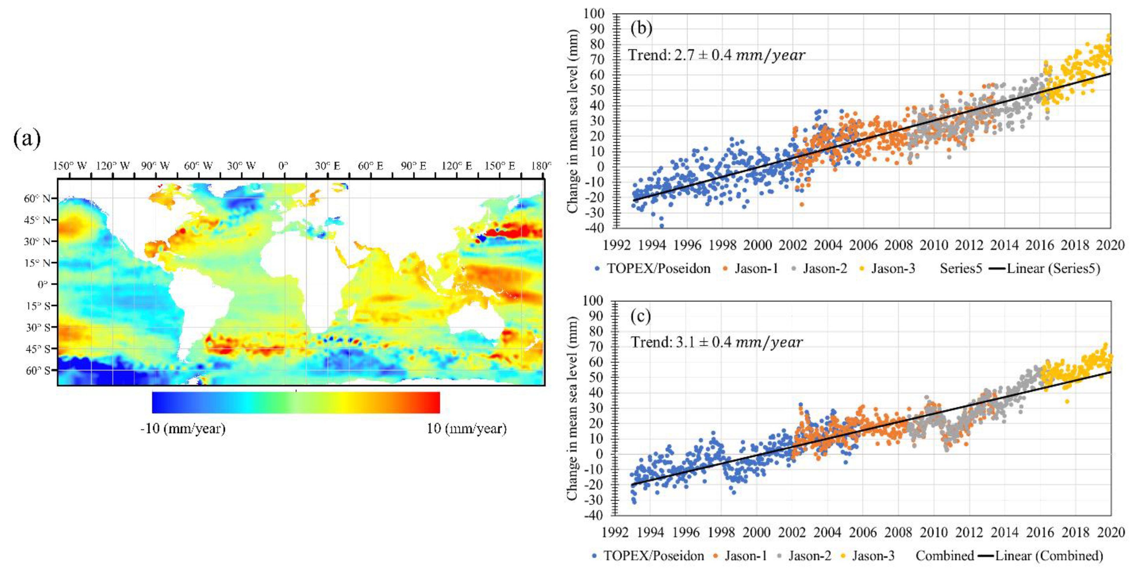
  213. Church, J.A.; White, N.J. Sea-level rise from the late 19th to the early 21st century. Surv. Geophys. 2011, 32, 585–602. [Google Scholar] [CrossRef] [Green Version]
  214. Palmer, M.D.; Harris, G.R.; Gregory, J.M. Extending CMIP5 projections of global mean temperature change and sea level rise due to thermal expansion using a physically-based emulator. Environ. Res. Lett. 2018, 13, 084003. [Google Scholar] [CrossRef]
  215. Frederikse, T.; Landerer, F.; Caron, L.; Adhikari, S.; Parkes, D.; Humphrey, V.W.; Dangendorf, S.; Hogarth, P.; Zanna, L.; Cheng, L. The causes of sea-level rise since 1900. Nature 2020, 584, 393–397. [Google Scholar] [CrossRef]
  216. Feng, W.; Shum, C.; Zhong, M.; Pan, Y. Groundwater storage changes in China from satellite gravity: An overview. Remote Sens. 2018, 10, 674. [Google Scholar] [CrossRef] [Green Version]
  217. Tuck, M.E.; Kench, P.S.; Ford, M.R.; Masselink, G. Physical modelling of the response of reef islands to sea-level rise. Geology 2019, 47, 803–806. [Google Scholar] [CrossRef]
  218. Reineman, D.R.; Thomas, L.N.; Caldwell, M.R. Using local knowledge to project sea level rise impacts on wave resources in California. Ocean Coast. Manag. 2017, 138, 181–191. [Google Scholar] [CrossRef]
  219. Sahin, O.; Stewart, R.A.; Faivre, G.; Ware, D.; Tomlinson, R.; Mackey, B. Spatial Bayesian Network for predicting sea level rise induced coastal erosion in a small Pacific Island. J. Environ. Manag. 2019, 238, 341–351. [Google Scholar] [CrossRef]
  220. Meyer, R.; Engesgaard, P.; Sonnenborg, T.O. Origin and dynamics of saltwater intrusion in a regional aquifer: Combining 3-D saltwater modeling with geophysical and geochemical data. Water Resour. Res. 2019, 55, 1792–1813. [Google Scholar] [CrossRef] [Green Version]
  221. Varela, M.R.; Patrício, A.R.; Anderson, K.; Broderick, A.C.; DeBell, L.; Hawkes, L.A.; Tilley, D.; Snape, R.T.; Westoby, M.J.; Godley, B.J. Assessing climate change associated sea-level rise impacts on sea turtle nesting beaches using drones, photogrammetry and a novel GPS system. Glob. Change Biol. 2019, 25, 753–762. [Google Scholar] [CrossRef]
  222. Kheir, A.M.; El Baroudy, A.; Aiad, M.A.; Zoghdan, M.G.; Abd El-Aziz, M.A.; Ali, M.G.; Fullen, M.A. Impacts of rising temperature, carbon dioxide concentration and sea level on wheat production in North Nile delta. Sci. Total Environ. 2019, 651, 3161–3173. [Google Scholar] [CrossRef]
  223. Carvalho, K.; Wang, S. Characterizing the Indian Ocean sea level changes and potential coastal flooding impacts under global warming. J. Hydrol. 2019, 569, 373–386. [Google Scholar] [CrossRef]
  224. Christodoulou, A.; Christidis, P.; Demirel, H. Sea-level rise in ports: A wider focus on impacts. Marit. Econ. Logist. 2019, 21, 482–496. [Google Scholar] [CrossRef]
  225. Parker, V.T.; Boyer, K.E. Sea-level rise and climate change impacts on an urbanized Pacific Coast estuary. Wetlands 2019, 39, 1219–1232. [Google Scholar] [CrossRef]
  226. Oral, N. International Law as an Adaptation Measure to Sea-level Rise and Its Impacts on Islands and Offshore Features. Int. J. Mar. Coast. Law 2019, 34, 415–439. [Google Scholar] [CrossRef]
  227. Lafta, A.A.; Altaei, S.A.; Al-Hashimi, N.H. Impacts of potential sea-level rise on tidal dynamics in Khor Abdullah and Khor Al-Zubair, northwest of Arabian Gulf. Earth Syst. Environ. 2020, 4, 93–105. [Google Scholar] [CrossRef]
  228. Dill, R.; Dobslaw, H. Seasonal variations in global mean sea level and consequences on the excitation of length-of-day changes. Geophys. J. Int. 2019, 218, 801–816. [Google Scholar] [CrossRef]
  229. Lowe, S.T.; Zuffada, C.; Chao, Y.; Kroger, P.; Young, L.E.; LaBrecque, J.L. 5-cm-Precision aircraft ocean altimetry using GPS reflections. Geophys. Res. Lett. 2002, 29, 13-11–13-14. [Google Scholar] [CrossRef] [Green Version]
  230. Jeon, T.; Seo, K.-W.; Youm, K.; Chen, J.; Wilson, C.R. Global sea level change signatures observed by GRACE satellite gravimetry. Sci. Rep. 2018, 8, 13519. [Google Scholar] [CrossRef] [Green Version]
  231. Quartly, G.D.; Rinne, E.; Passaro, M.; Andersen, O.B.; Dinardo, S.; Fleury, S.; Guillot, A.; Hendricks, S.; Kurekin, A.A.; Müller, F.L. Retrieving sea level and freeboard in the Arctic: A review of current radar altimetry methodologies and future perspectives. Remote Sens. 2019, 11, 881. [Google Scholar] [CrossRef]
  232. Balogun, A.-L.; Adebisi, N. Sea level prediction using ARIMA, SVR and LSTM neural network: Assessing the impact of ensemble Ocean-Atmospheric processes on models’ accuracy. Geomat. Nat. Hazards Risk 2021, 12, 653–674. [Google Scholar] [CrossRef]
  233. Nieves, V.; Radin, C.; Camps-Valls, G. Predicting regional coastal sea level changes with machine learning. Sci. Rep. 2021, 11, 7650. [Google Scholar] [CrossRef]
  234. Chupin, C.; Ballu, V.; Testut, L.; Tranchant, Y.-T.; Calzas, M.; Poirier, E.; Coulombier, T.; Laurain, O.; Bonnefond, P.; Project, T.F. Mapping sea surface height using new concepts of kinematic GNSS instruments. Remote Sens. 2020, 12, 2656. [Google Scholar] [CrossRef]
  235. Clarizia, M.P.; Ruf, C.; Cipollini, P.; Zuffada, C. First spaceborne observation of sea surface height using GPS-Reflectometry. Geophys. Res. Lett. 2016, 43, 767–774. [Google Scholar] [CrossRef] [Green Version]
  236. Gleason, S.; Gebre-Egziabher, D.; Egziabher, D.G. GNSS Applications and Methods; Artech House: Norwood, MA, USA, 2009. [Google Scholar]
  237. Martin-Neira, M. A passive reflectometry and interferometry system (PARIS): Application to ocean altimetry. ESA J. 1993, 17, 331–355. [Google Scholar]
  238. Hajj, G.A.; Zuffada, C. Theoretical description of a bistatic system for ocean altimetry using the GPS signal. Radio Sci. 2003, 38, 10-11–10-19. [Google Scholar] [CrossRef]
  239. Cardellach, E.; Rius, A.; Martín-Neira, M.; Fabra, F.; Nogues-Correig, O.; Ribó, S.; Kainulainen, J.; Camps, A.; D'Addio, S. Consolidating the precision of interferometric GNSS-R ocean altimetry using airborne experimental data. IEEE Trans. Geosci. Remote Sens. 2013, 52, 4992–5004. [Google Scholar] [CrossRef]
  240. Camps, A.; Park, H.; i Domènech, E.V.; Pascual, D.; Martin, F.; Rius, A.; Ribo, S.; Benito, J.; Andrés-Beivide, A.; Saameno, P. Optimization and performance analysis of interferometric GNSS-R altimeters: Application to the PARIS IoD mission. IEEE J. Sel. Top. Appl. Earth Obs. Remote Sens. 2014, 7, 1436–1451. [Google Scholar] [CrossRef]
  241. Wang, Q.; Zheng, W.; Wu, F.; Xu, A.; Zhu, H.; Liu, Z. A New GNSS-R Altimetry Algorithm Based on Machine Learning Fusion Model and Feature Optimization to Improve the Precision of Sea Surface Height Retrieval. Front. Earth Sci. 2021, 758. [Google Scholar] [CrossRef]
  242. Taqi, A.M.; Al-Subhi, A.M.; Alsaafani, M.A.; Abdulla, C.P. Improving sea level anomaly precision from satellite altimetry using parameter correction in the Red Sea. Remote Sens. 2020, 12, 764. [Google Scholar] [CrossRef] [Green Version]
  243. Fernandes, M.J.; Lázaro, C.; Ablain, M.; Pires, N. Improved wet path delays for all ESA and reference altimetric missions. Remote Sens. Environ. 2015, 169, 50–74. [Google Scholar] [CrossRef]
  244. Carrere, L.; Faugère, Y.; Ablain, M. Major improvement of altimetry sea level estimations using pressure-derived corrections based on ERA-Interim atmospheric reanalysis. Ocean Sci. 2016, 12, 825–842. [Google Scholar] [CrossRef] [Green Version]
  245. Carrere, L.; Lyard, F.; Cancet, M.; Guillot, A. FES 2014, a new tidal model on the global ocean with enhanced accuracy in shallow seas and in the Arctic region. In Proceedings of the EGU General Assembly 2015, Vienna, Austria, 12–17 April 2015. [Google Scholar]
  246. Passaro, M.; Nadzir, Z.A.; Quartly, G.D. Improving the precision of sea level data from satellite altimetry with high-frequency and regional sea state bias corrections. Remote Sens. Environ. 2018, 218, 245–254. [Google Scholar] [CrossRef] [Green Version]
  247. Ren, L.; Yang, J.; Dong, X.; Zhang, Y.; Jia, Y. Preliminary Evaluation and Correction of Sea Surface Height from Chinese Tiangong-2 Interferometric Imaging Radar Altimeter. Remote Sens. 2020, 12, 2496. [Google Scholar] [CrossRef]
  248. Dinardo, S.; Fenoglio-Marc, L.; Buchhaupt, C.; Becker, M.; Scharroo, R.; Fernandes, M.J.; Benveniste, J. Coastal sar and plrm altimetry in german bight and west baltic sea. Adv. Space Res. 2018, 62, 1371–1404. [Google Scholar] [CrossRef]
  249. Mullick, M.R.A.; Tanim, A.; Islam, S.S. Coastal vulnerability analysis of Bangladesh coast using fuzzy logic based geospatial techniques. Ocean Coast. Manag. 2019, 174, 154–169. [Google Scholar] [CrossRef]
  250. Yang, L.; Jin, T.; Gao, X.; Wen, H.; Schöne, T.; Xiao, M.; Huang, H. Sea Level Fusion of Satellite Altimetry and Tide Gauge Data by Deep Learning in the Mediterranean Sea. Remote Sens. 2021, 13, 908. [Google Scholar] [CrossRef]
  251. Bindoff, N.L.; Willebrand, J.; Artale, V.; Cazenave, A.; Gregory, J.; Gulev, S.; Hanawa, K.; Le Quéré, C.; Levitus, S.; Nojiri, Y.; et al. 007: Observations: Oceanic Climate Change and Sea Level. In Climate Change 2007: The Physical Science Basis. Contribution of Working Group I to the Fourth Assessment Report of the Intergovernmental Panel on Climate Change; Solomon, S.D., Qin, M., Manning, Z., Chen, M., Marquis, K.B., Averyt, M.T., Miller, H.L., Eds.; Cambridge University Press: Cambridge, UK; New York, NY, USA.
  252. Chen, J.; Tapley, B.; Seo, K.W.; Wilson, C.; Ries, J. Improved quantification of global mean ocean mass change using GRACE satellite gravimetry measurements. Geophys. Res. Lett. 2019, 46, 13984–13991. [Google Scholar] [CrossRef]
  253. Cazenave, A.; Dominh, K.; Guinehut, S.; Berthier, E.; Llovel, W.; Ramillien, G.; Ablain, M.; Larnicol, G. Sea level budget over 2003–2008: A reevaluation from GRACE space gravimetry, satellite altimetry and Argo. Glob. Planet. Change 2009, 65, 83–88. [Google Scholar] [CrossRef] [Green Version]
  254. Elsaka, B.; Radwan, A.M.; Rashwan, M. Evaluation of Nile Delta-Mediterranean Sea conjunction using GPS, satellite-based gravity and altimetry datasets. J. Geosci. Environ. Prot. 2020, 8, 33. [Google Scholar] [CrossRef] [Green Version]
  255. Drogoudi, P.D.; Tsipouridis, C.; Michailidis, Z. Physical and chemical characteristics of pomegranates. HortScience 2005, 40, 1200–1203. [Google Scholar] [CrossRef]
  256. Roadmap, T. Welcome to Tides and Water Levels. Available online: https://oceanservice.noaa.gov/education/tutorial_tides/welcome.htmldate (accessed on 5 September 2022).
  257. Taylor, G.I.I. Tidal friction in the Irish Sea. Philos. Trans. R. Soc. London. Ser. A Contain. Pap. A Math. Or Phys. Character 1920, 220, 1–33. [Google Scholar]
  258. Jeffreys, H., VIII. Tidal friction in shallow seas. Philos. Trans. R. Soc. London. Ser. A Contain. Pap. A Math. Or Phys. Character 1921, 221, 239–264. [Google Scholar]
  259. Cartwright, D.E.; Ray, R. Oceanic tides from Geosat altimetry. J. Geophys. Res. Ocean. 1990, 95, 3069–3090. [Google Scholar] [CrossRef]
  260. Egbert, G.; Ray, R. Significant dissipation of tidal energy in the deep ocean inferred from satellite altimeter data. Nature 2000, 405, 775–778. [Google Scholar] [CrossRef] [PubMed]
  261. Tierney, C.C.; Kantha, L.H.; Born, G.H. Shallow and deep water global ocean tides from altimetry and numerical modeling. J. Geophys. Res. Ocean. 2000, 105, 11259–11277. [Google Scholar] [CrossRef]
  262. Ryu, J.-H.; Choi, J.-K.; Lee, Y.-K. Potential of remote sensing in management of tidal flats: A case study of thematic mapping in the Korean tidal flats. Ocean Coast. Manag. 2014, 102, 458–470. [Google Scholar] [CrossRef]
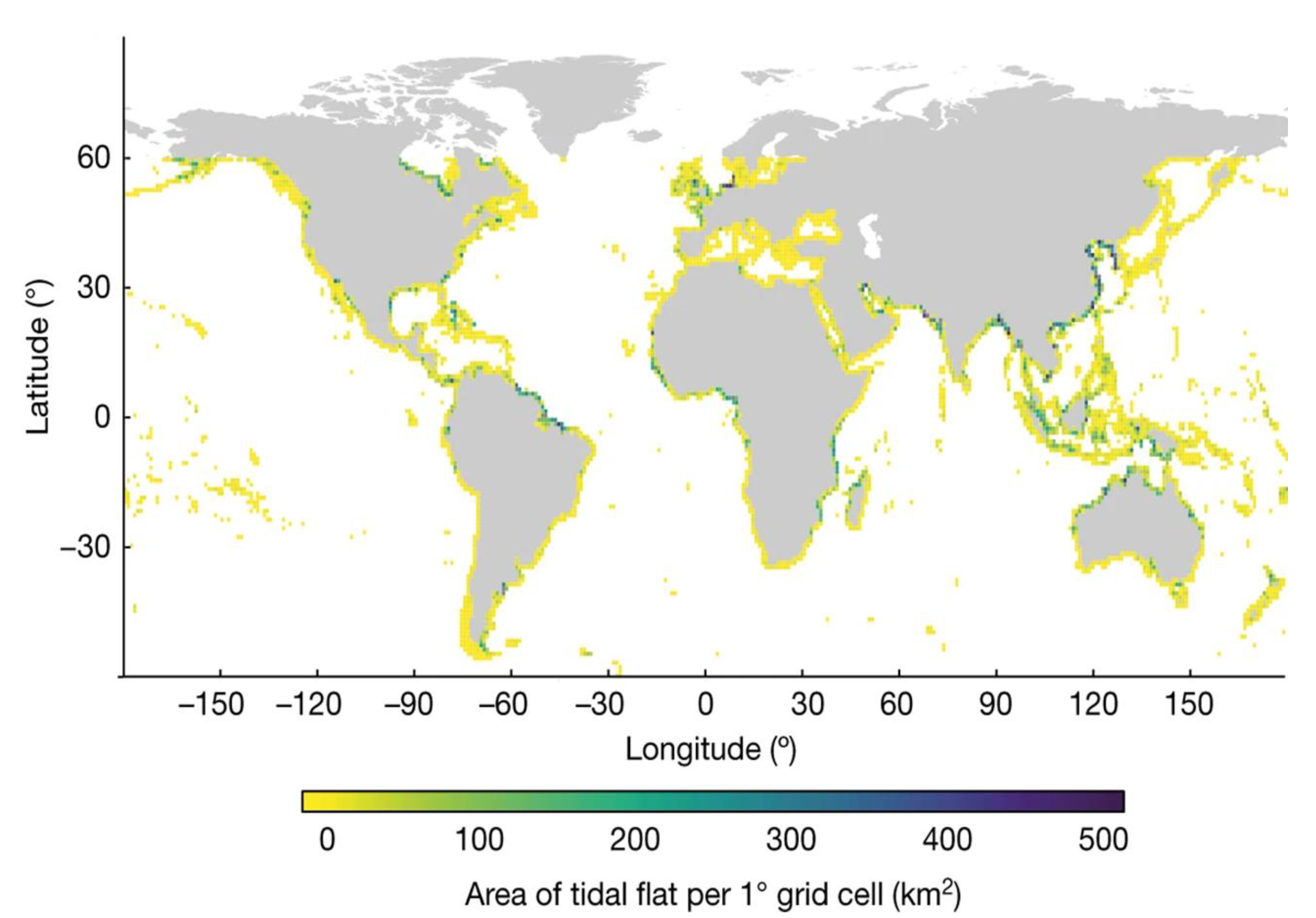
  263. Murray, N.J.; Phinn, S.R.; DeWitt, M.; Ferrari, R.; Johnston, R.; Lyons, M.B.; Clinton, N.; Thau, D.; Fuller, R.A. The global distribution and trajectory of tidal flats. Nature 2019, 565, 222–225. [Google Scholar] [CrossRef] [PubMed]
  264. Gade, M.; Alpers, W.; Melsheimer, C.; Tanck, G. Classification of sediments on exposed tidal flats in the German Bight using multi-frequency radar data. Remote Sens. Environ. 2008, 112, 1603–1613. [Google Scholar] [CrossRef]
  265. Lee, J.K.; Lee, I.; Kim, J.O. Analysis on tidal channels based on UAV photogrammetry: Focused on the west coast, South Korea case analysis. J. Coast. Res. 2017, 199–203. [Google Scholar] [CrossRef] [Green Version]
  266. Mason, D.C.; Scott, T.R.; Wang, H.-J. Extraction of tidal channel networks from airborne scanning laser altimetry. ISPRS J. Photogramm. Remote Sens. 2006, 61, 67–83. [Google Scholar] [CrossRef]
  267. Letcher, T.M. Future Energy: Improved, Sustainable and Clean Options for Our Planet; Elsevier: The Netherlands, 2008. [Google Scholar]
  268. Du, T.; Tseng, Y.H.; Yan, X.H. Impacts of tidal currents and Kuroshio intrusion on the generation of nonlinear internal waves in Luzon Strait. J. Geophys. Res. Ocean. 2008, 113, C08015. [Google Scholar] [CrossRef]
  269. Ferreira, R.M.; Estefen, S.F.; Romeiser, R. Under what conditions sar along-track interferometry is suitable for assessment of tidal energy resource. IEEE J. Sel. Top. Appl. Earth Obs. Remote Sens. 2016, 9, 5011–5022. [Google Scholar] [CrossRef]
  270. Tsai, C.-H.; Doong, D.-J.; Chen, Y.-C.; Yen, C.-W.; Maa, M.J. Tidal stream characteristics on the coast of Cape Fuguei in northwestern Taiwan for a potential power generation site. Int. J. Mar. Energy 2016, 13, 193–205. [Google Scholar] [CrossRef]
  271. Schubert, G. (Ed.) Treatise on Geophysics, 2nd ed.; Elsevier: Amsterdam, The Netherlands, 2015. [Google Scholar]
  272. Kelly, M.; Tuxen, K. Remote sensing support for tidal wetland vegetation research and management. In Remote Sensing and Geospatial Technologies for Coastal Ecosystem Assessment and Management; Springer: Berlin/Heidelberg, Germany, 2009; pp. 341–363. [Google Scholar]
  273. Magolan, J.L.; Halls, J.N. A multi-decadal investigation of tidal creek wetland changes, water level rise, and ghost forests. Remote Sens. 2020, 12, 1141. [Google Scholar] [CrossRef] [Green Version]
  274. Slatton, K.C.; Crawford, M.M.; Chang, L.-D. Modeling temporal variations in multipolarized radar scattering from intertidal coastal wetlands. ISPRS J. Photogramm. Remote Sens. 2008, 63, 559–577. [Google Scholar] [CrossRef]
  275. Wang, C.; Liu, H.-Y.; Zhang, Y.; Li, Y.-f. Classification of land-cover types in muddy tidal flat wetlands using remote sensing data. J. Appl. Remote Sens. 2014, 7, 073457. [Google Scholar] [CrossRef] [Green Version]
  276. Whyte, A.; Ferentinos, K.P.; Petropoulos, G.P. A new synergistic approach for monitoring wetlands using Sentinels-1 and 2 data with object-based machine learning algorithms. Environ. Model. Softw. 2018, 104, 40–54. [Google Scholar] [CrossRef] [Green Version]
  277. Ryu, J.-H.; Won, J.-S.; Min, K.D. Waterline extraction from Landsat TM data in a tidal flat: A case study in Gomso Bay, Korea. Remote Sens. Environ. 2002, 83, 442–456. [Google Scholar] [CrossRef]
  278. Murray, N.J.; Phinn, S.R.; Clemens, R.S.; Roelfsema, C.M.; Fuller, R.A. Continental scale mapping of tidal flats across East Asia using the Landsat archive. Remote Sens. 2012, 4, 3417–3426. [Google Scholar] [CrossRef] [Green Version]
  279. Zhao, Y.; Liu, Q.; Huang, R.; Pan, H.; Xu, M. Recent Evolution of Coastal Tidal Flats and the Impacts of Intensified Human Activities in the Modern Radial Sand Ridges, East China. Int. J. Environ. Res. Public Health 2020, 17, 3191. [Google Scholar] [CrossRef] [PubMed]
  280. Angeles, G.R.; Perillo, G.M.; Piccolo, M.C.; Pierini, J.O. Fractal analysis of tidal channels in the Bahıa Blanca Estuary (Argentina). Geomorphology 2004, 57, 263–274. [Google Scholar] [CrossRef]
  281. Mahdavi, S.; Salehi, B.; Granger, J.; Amani, M.; Brisco, B.; Huang, W. Remote sensing for wetland classification: A comprehensive review. GIScience Remote Sens. 2018, 55, 623–658. [Google Scholar] [CrossRef]
  282. Amani, M.; Mahdavi, S.; Berard, O. Supervised wetland classification using high spatial resolution optical, SAR, and LiDAR imagery. J. Appl. Remote Sens. 2020, 14, 024502. [Google Scholar] [CrossRef]
  283. Mahdavi, S.; Salehi, B.; Amani, M.; Granger, J.; Brisco, B.; Huang, W. A dynamic classification scheme for mapping spectrally similar classes: Application to wetland classification. Int. J. Appl. Earth Obs. Geoinf. 2019, 83, 101914. [Google Scholar] [CrossRef]
  284. Kleinherenbrink, M.; Riva, R.; Frederikse, T. A comparison of methods to estimate vertical land motion trends from GNSS and altimetry at tide gauge stations. Ocean Sci. 2018, 14, 187–204. [Google Scholar] [CrossRef] [Green Version]
  285. Takiguchi, H.; Otsubo, T.; Fukuda, Y. Reduction of influences of the earth's Surface Fluid Loads on GPS Site Coordinate Time Series and Global Satellite Laser Ranging Analysis. 2006. Available online: https://openrepository.aut.ac.nz/handle/10292/3985 (accessed on 12 January 2022).
  286. Zhou, M.; Liu, X.; Guo, J.; Jin, X.; Chang, X. Ocean Tide Loading Displacement Parameters Estimated From GNSS-Derived Coordinate Time Series Considering the Effect of Mass Loading in Hong Kong. IEEE J. Sel. Top. Appl. Earth Obs. Remote Sens. 2020, 13, 6064–6076. [Google Scholar] [CrossRef]
  287. MirMazloumi, S.M.; Sahebi, M.R. Assessment of different backscattering models for bare soil surface parameters estimation from SAR data in band C, L and P. Eur. J. Remote Sens. 2016, 49, 261–278. [Google Scholar] [CrossRef] [Green Version]
  288. Heygster, G.; Dannenberg, J.; Notholt, J. Topographic mapping of the German tidal flats analyzing SAR images with the waterline method. IEEE Trans. Geosci. Remote Sens. 2009, 48, 1019–1030. [Google Scholar] [CrossRef]
  289. Lamont-Smith, T.; Dovey, P. The effect of tidal currents on radar backscatter from the sea around Portland Bill. Int. J. Remote Sens. 2005, 26, 2061–2079. [Google Scholar] [CrossRef]
  290. Ren, Y.; Li, X.-M.; Gao, G.; Busche, T.E. Derivation of sea surface tidal current from spaceborne SAR constellation data. IEEE Trans. Geosci. Remote Sens. 2017, 55, 3236–3247. [Google Scholar] [CrossRef] [Green Version]
  291. DiCaprio, C.J.; Simons, M. Importance of ocean tidal load corrections for differential InSAR. Geophys. Res. Lett. 2008, 35, L22309. [Google Scholar] [CrossRef] [Green Version]
  292. Peng, W.; Wang, Q.; Cao, Y. Analysis of ocean tide loading in differential InSAR measurements. Remote Sens. 2017, 9, 101. [Google Scholar] [CrossRef]
  293. Wdowinski, S.; Hong, S.-H.; Mulcan, A.; Brisco, B. Remote-sensing monitoring of tide propagation through coastal wetlands. Oceanography 2013, 26, 64–69. [Google Scholar] [CrossRef] [Green Version]
  294. Amani, M.; Salehi, B.; Mahdavi, S.; Brisco, B.; Shehata, M. A Multiple Classifier System to improve mapping complex land covers: A case study of wetland classification using SAR data in Newfoundland, Canada. Int. J. Remote Sens. 2018, 39, 7370–7383. [Google Scholar] [CrossRef]
  295. Mahdavi, S.; Salehi, B.; Amani, M.; Granger, J.E.; Brisco, B.; Huang, W.; Hanson, A. Object-based classification of wetlands in Newfoundland and Labrador using multi-temporal PolSAR data. Can. J. Remote Sens. 2017, 43, 432–450. [Google Scholar] [CrossRef]
  296. Egbert, G.D.; Ray, R.D. Tidal prediction. J. Mar. Res. 2017, 75, 189–237. [Google Scholar] [CrossRef]
  297. Ray, R.D.; Zaron, E.D. Non-stationary internal tides observed with satellite altimetry. Geophys. Res. Lett. 2011, 38, L17609. [Google Scholar] [CrossRef] [Green Version]
  298. Chen, L. Detection of shoreline changes for tideland areas using multi-temporal satellite images. Int. J. Remote Sens. 1998, 19, 3383–3397. [Google Scholar] [CrossRef]
  299. Tseng, K.-H.; Kuo, C.-Y.; Lin, T.-H.; Huang, Z.-C.; Lin, Y.-C.; Liao, W.-H.; Chen, C.-F. Reconstruction of time-varying tidal flat topography using optical remote sensing imageries. ISPRS J. Photogramm. Remote Sens. 2017, 131, 92–103. [Google Scholar] [CrossRef]
  300. Mason, D.; Scott, T.; Dance, S. Remote sensing of intertidal morphological change in Morecambe Bay, UK, between 1991 and 2007. Estuar. Coast. Shelf Sci. 2010, 87, 487–496. [Google Scholar] [CrossRef] [Green Version]
  301. Passaro, M.; Fenoglio-Marc, L.; Cipollini, P. Validation of significant wave height from improved satellite altimetry in the German Bight. IEEE Trans. Geosci. Remote Sens. 2014, 53, 2146–2156. [Google Scholar] [CrossRef]
  302. Yu, H.; Li, J.; Wu, K.; Wang, Z.; Yu, H.; Zhang, S.; Hou, Y.; Kelly, R.M. A global high-resolution ocean wave model improved by assimilating the satellite altimeter significant wave height. Int. J. Appl. Earth Obs. Geoinf. 2018, 70, 43–50. [Google Scholar] [CrossRef]
  303. Lee, M.; Oh, N.; Kim, G.; Kang, J. Modeling tidal current around mokpo, the south western coastal zone of korea. In Proceedings of the the 7th International Conference on Asian and Pacific Coasts, Bali, Indonesia, 24–26 September 2013; pp. 521–526. [Google Scholar]
  304. Green, J.; Pugh, D.T. Bardsey–an island in a strong tidal stream: Underestimating coastal tides due to unresolved topography. Ocean Sci. 2020, 16, 1337–1345. [Google Scholar] [CrossRef]
  305. Niedermeier, A.; Hoja, D.; Lehner, S. Topography and morphodynamics in the German Bight using SAR and optical remote sensing data. Ocean Dyn. 2005, 55, 100–109. [Google Scholar] [CrossRef]
  306. Anthony, E.J.; Dolique, F.; Gardel, A.; Gratiot, N.; Proisy, C.; Polidori, L. Nearshore intertidal topography and topographic-forcing mechanisms of an Amazon-derived mud bank in French Guiana. Cont. Shelf Res. 2008, 28, 813–822. [Google Scholar] [CrossRef]
  307. Ryu, J.-H.; Kim, C.-H.; Lee, Y.-K.; Won, J.-S.; Chun, S.-S.; Lee, S. Detecting the intertidal morphologic change using satellite data. Estuar. Coast. Shelf Sci. 2008, 78, 623–632. [Google Scholar] [CrossRef]
  308. Lee, Y.-K.; Ryu, J.-H.; Choi, J.-K.; Soh, J.-G.; Eom, J.-A.; Won, J.-S. A study of decadal sedimentation trend changes by waterline comparisons within the Ganghwa tidal flats initiated by human activities. J. Coast. Res. 2011, 27, 857–869. [Google Scholar] [CrossRef]
  309. Kang, Y.; Ding, X.; Xu, F.; Zhang, C.; Ge, X. Topographic mapping on large-scale tidal flats with an iterative approach on the waterline method. Estuar. Coast. Shelf Sci. 2017, 190, 11–22. [Google Scholar] [CrossRef]
  310. Zhang, S.; Liu, Y.; Yang, Y.; Sun, C.; Li, F. Erosion and deposition within Poyang Lake: Evidence from a decade of satellite data. J. Great Lakes Res. 2016, 42, 364–374. [Google Scholar] [CrossRef]
  311. Lohani, B. Construction of a digital elevation model of the Holderness coast using the waterline method and airborne thematic mapper data. Int. J. Remote Sens. 1999, 20, 593–607. [Google Scholar] [CrossRef]
  312. Lohani, B.; Mason, D.C. Application of airborne scanning laser altimetry to the study of tidal channel geomorphology. ISPRS J. Photogramm. Remote Sens. 2001, 56, 100–120. [Google Scholar] [CrossRef]
  313. Corbane, C.; Najman, L.; Pecoul, E.; Demagistri, L.; Petit, M. A complete processing chain for ship detection using optical satellite imagery. Int. J. Remote Sens. 2010, 31, 5837–5854. [Google Scholar] [CrossRef]
  314. Zhu, C.; Zhou, H.; Wang, R.; Guo, J. A novel hierarchical method of ship detection from spaceborne optical image based on shape and texture features. IEEE Trans. Geosci. Remote Sens. 2010, 48, 3446–3456. [Google Scholar] [CrossRef]
  315. Bi, F.; Zhu, B.; Gao, L.; Bian, M. A visual search inspired computational model for ship detection in optical satellite images. IEEE Geosci. Remote Sens. Lett. 2012, 9, 749–753. [Google Scholar]
  316. Park, J.-J.; Oh, S.; Park, K.-A.; Foucher, P.-Y.; Jang, J.-C.; Lee, M.; Kim, T.-S.; Kang, W.-S. The ship detection using airborne and in-situ measurements based on hyperspectral remote sensing. J. Korean Earth Sci. Soc. 2017, 38, 535–545. [Google Scholar] [CrossRef]
  317. Yang, F.; Xu, Q.; Li, B.; Ji, Y. Ship detection from thermal remote sensing imagery through region-based deep forest. IEEE Geosci. Remote Sens. Lett. 2018, 15, 449–453. [Google Scholar] [CrossRef]
  318. Xu, C.; Zhang, D.; Zhang, Z.; Feng, Z. BgCut: Automatic Ship Detection from UAV Images. Sci. World J. 2014, 2014, 171978. [Google Scholar] [CrossRef] [Green Version]
  319. Yang, G.; Li, B.; Ji, S.; Gao, F.; Xu, Q. Ship detection from optical satellite images based on sea surface analysis. IEEE Geosci. Remote Sens. Lett. 2013, 11, 641–645. [Google Scholar] [CrossRef]
  320. Yang, X.; Sun, H.; Fu, K.; Yang, J.; Sun, X.; Yan, M.; Guo, Z. Automatic ship detection in remote sensing images from google earth of complex scenes based on multiscale rotation dense feature pyramid networks. Remote Sens. 2018, 10, 132. [Google Scholar] [CrossRef] [Green Version]
  321. Wang, N.; Li, B.; Xu, Q.; Wang, Y. Automatic ship detection in optical remote sensing images based on anomaly detection and SPP-PCANet. Remote Sens. 2018, 11, 47. [Google Scholar] [CrossRef] [Green Version]
  322. Girshick, R.; Donahue, J.; Darrell, T.; Malik, J. Region-based convolutional networks for accurate object detection and segmentation. IEEE Trans. Pattern Anal. Mach. Intell. 2015, 38, 142–158. [Google Scholar] [CrossRef]
  323. Girshick, R. Fast r-cnn. In Proceedings of the IEEE International Conference on Computer Vision; Santiago, Chile, 7–13 December 2015, pp. 1440–1448.
  324. Ren, S.; He, K.; Girshick, R.; Sun, J. Faster r-cnn: Towards real-time object detection with region proposal networks. Adv. Neural Inf. Process. Syst. 2015, 28. [Google Scholar] [CrossRef] [Green Version]
  325. Zhang, S.; Wu, R.; Xu, K.; Wang, J.; Sun, W. R-CNN-based ship detection from high resolution remote sensing imagery. Remote Sens. 2019, 11, 631. [Google Scholar] [CrossRef]
  326. Tang, J.; Deng, C.; Huang, G.-B.; Zhao, B. Compressed-domain ship detection on spaceborne optical image using deep neural network and extreme learning machine. IEEE Trans. Geosci. Remote Sens. 2014, 53, 1174–1185. [Google Scholar] [CrossRef]
  327. Kanjir, U.; Greidanus, H.; Oštir, K. Vessel detection and classification from spaceborne optical images: A literature survey. Remote Sens. Environ. 2018, 207, 1–26. [Google Scholar] [CrossRef] [PubMed]
  328. Zhang, W.; Bian, C.; Zhao, X.; Hou, Q. Ship target segmentation and detection in complex optical remote sensing image based on component tree characteristics discrimination. In Optoelectronic Imaging and Multimedia Technology II; SPIE: Bellingham, WA, USA, 2012; Volume 8558, pp. 502–510. [Google Scholar]
  329. Proia, N.; Pagé, V. Characterization of a Bayesian ship detection method in optical satellite images. IEEE Geosci. Remote Sens. Lett. 2009, 7, 226–230. [Google Scholar] [CrossRef]
  330. Qi, S.; Ma, J.; Lin, J.; Li, Y.; Tian, J. Unsupervised ship detection based on saliency and S-HOG descriptor from optical satellite images. IEEE Geosci. Remote Sens. Lett. 2015, 12, 1451–1455. [Google Scholar]
  331. Ringrose, R.; Harris, N. Ship detection using polarimetric SAR data. In SAR Workshop; CEOS Committee on Earth Observation Satellites: Toulouse, France, 1999; p. 687. [Google Scholar]
  332. Touzi, R.; Charbonneau, F.; Hawkins, R.; Murnaghan, K.; Kavoun, X. Ship-sea contrast optimization when using polarimetric SARs. In Proceedings of the IGARSS 2001. Scanning the Present and Resolving the Future. Proceedings. IEEE 2001 International Geoscience and Remote Sensing Symposium (Cat. No. 01CH37217), Sydney, NSW, Australia, 9–13 July 2001; pp. 426–428. [Google Scholar]
  333. Tello, M.; López-Martínez, C.; Mallorquí, J.J.; Greidanus, H. A novel algorithm for ship detection in Envisat SAR imagery based on the wavelet transform. IEEE Geosci. Remote Sens. Lett. 2005, 2, 201–205. [Google Scholar] [CrossRef]
  334. Iervolino, P.; Guida, R. A novel ship detector based on the generalized-likelihood ratio test for SAR imagery. IEEE J. Sel. Top. Appl. Earth Obs. Remote Sens. 2017, 10, 3616–3630. [Google Scholar] [CrossRef] [Green Version]
  335. Crisp, D.J. The State-of-the-Art in Ship Detection in Synthetic Aperture Radar Imagery; Defence Science and Technology Organisation; DSTO information Sciences Laboratory: Edinburg, South Australia, 2004. [Google Scholar]
  336. Leng, X.; Ji, K.; Yang, K.; Zou, H. A bilateral CFAR algorithm for ship detection in SAR images. IEEE Geosci. Remote Sens. Lett. 2015, 12, 1536–1540. [Google Scholar] [CrossRef]
  337. Wang, C.; Bi, F.; Zhang, W.; Chen, L. An intensity-space domain CFAR method for ship detection in HR SAR images. IEEE Geosci. Remote Sens. Lett. 2017, 14, 529–533. [Google Scholar] [CrossRef]
  338. Jiao, J.; Zhang, Y.; Sun, H.; Yang, X.; Gao, X.; Hong, W.; Fu, K.; Sun, X. A densely connected end-to-end neural network for multiscale and multiscene SAR ship detection. IEEE Access 2018, 6, 20881–20892. [Google Scholar] [CrossRef]
  339. Nazari, M.E.; Ghorbani, A. Predicting a Three-Dimensional Radar Coverage Area: Introducing a new method based on propagation of radio waves. IEEE Antennas Propag. Mag. 2016, 58, 28–34. [Google Scholar] [CrossRef]
  340. Shearman, E. Propagation and scattering in MF/HF groundwave radar. In IEE Proceedings F (Communications, Radar and Signal Processing). IET Digital Library, 1983; 590, p. 579. Available online: https://ui.adsabs.harvard.edu/abs/1983IPCRS.130..579S/abstractdate (accessed on 5 September 2022).
  341. Dzvonkovskaya, A.; Rohling, H. HF radar ship detection and tracking using WERA system. In Proceedings of the IET International Conference on Radar Systems 2007, Edinburgh, UK, 15–18 October 2007. [Google Scholar]
  342. Kendall, M.G. The Advanced Theory of Statistics, 2nd ed.; Charles Griffin & Co.: London, UK, 1946. [Google Scholar]
  343. Gorski, T.; Le Caillec, J.-M.; Kawalec, A.; Czarnecki, W.; Lennon, M.; Thomas, N. Target detection using HF radar data. In Proceedings of the OCEANS 2007-Europe, Aberdeen, UK, 18–21 June 2007; pp. 1–5. [Google Scholar]
  344. Roarty, H.; Barrick, D.; Kohut, J.; Glenn, S. Dual-use of compact HF radars for the detection of mid-and large-size vessels. Turk. J. Electr. Eng. Comput. Sci. 2010, 18, 373–388. [Google Scholar] [CrossRef]
  345. Park, S.; Cho, C.J.; Ku, B.; Lee, S.; Ko, H. Simulation and ship detection using surface radial current observing compact HF radar. IEEE J. Ocean. Eng. 2016, 42, 544–555. [Google Scholar] [CrossRef]
  346. Hong, Z.; Yang, T.; Tong, X.; Zhang, Y.; Jiang, S.; Zhou, R.; Han, Y.; Wang, J.; Yang, S.; Liu, S. Multi-Scale Ship Detection From SAR and Optical Imagery Via A More Accurate YOLOv3. IEEE J. Sel. Top. Appl. Earth Obs. Remote Sens. 2021, 14, 6083–6101. [Google Scholar] [CrossRef]
Figure 1. Overview of the met-ocean applications of RS which are discussed in this review paper.
Water 14 03400 g001
Figure 2. The spatial distribution of the global mean (a) OSW speeds and (b) wind power densities at 10 m above SL derived by a combination of QuikSCAT, Windsat, and ASCAT datasets from 1999 to 2015. The figure is directly adopted from Reference [103].
Water 14 03400 g002
Figure 3. The global ocean currents, including warm currents (red line), cold currents (blue line), and neutral current (black line) adopted from https://commons.wikimedia.org/wiki/File:Corrientes-oceanicas.png (accessed on 8 October 2022).
Water 14 03400 g003
Figure 4. Different methods for ocean current estimation.
Water 14 03400 g004
Figure 5. The locations of the global HF radar network.
Water 14 03400 g005
Figure 6. (a) Outline of the WaMoS II setting up, (b) sample of a WaMoS II X-band radar backscatter image, and (c) its bathymetry and current field at Tongue Point, Cape Terawhiti, New Zealand. The white arrows in (b) and black arrows in (c) show the peak wave direction of the incoming waves and the current vectors, respectively. The figure is directly adopted from References [73,121].
Water 14 03400 g006
Figure 7. (a) Global SL change between 1993 and 2022. Regional mean SL changes and trends of (b) the Atlantic Ocean and (c) the Pacific Ocean calculated from a combination of TOPEX/Poseidon, Jason-1, Jason-2, and Jason-3 satellite altimetry datasets. Satellite altimetry data were downloaded from [211].
Water 14 03400 g007
Figure 8. Global distribution of tidal flats during 2014–2016. The figure is directly adopted from Reference [9].
Water 14 03400 g008
Figure 9. A general ship detection method using spaceborne RS data.
Water 14 03400 g009
Table 1. Different RS systems for OSW estimation along with their advantages and disadvantages.
RS System (Passive/Active)RS System (Type)AdvantageDisadvantage
PassiveMicrowave radiometer Appropriate efficiency in high wind speeds, large-scale coverageLow accuracy for OSW direction estimation in low wind speeds, coarse spatial resolution
GNSS-RHigher spatial and temporal resolution, less sensitivity atmospheric attenuation, low-cost, low weight, low power needs for receivers, unique sensing geometryInadequate number of satellites, need more investigation and validation
ActiveSARHigh spatial resolution, applicable at both low and high wind speedsSpeckle noise issue, challenging preprocessing steps
ScatterometerGood efficiency in low wind speeds, global coverageCoarse spatial resolution, saturated signal in high wind speeds, rain contamination
HF radarReasonable accuracy at different wind speeds, large-scale coverageAvailability of OSW data only at specific coastal locations where the HF radar has been installed
Table 2. Different RS systems for OSC estimation along with their advantages and limitations.
RS System (Passive/Active)RS System (Type)AdvantageDisadvantage
PassiveOpticalProvides high spatial resolution images for retrieving and characterizing spatiotemporal OSCCalibrating issues due to defining several input parameters, limited by cloud cover, requires a reliable operational procedure for feature tracking, not suitable for nighttime
TIR
radiometers
Mesoscale OSC fields retrieval based on the feature tracking at high temporal rates Limited by cloud cover, edge-of-scan distortions, hard for features to evolve due to degradation of their surface signature
Microwave radiometersCan measure under clouds and in all weather conditions except for rain, OSC estimation at a global scaleCoarse resolution, limited to regions with sun-glitter, rain, or proximity to land
ActiveSARNot limited by cloud cover or daytime, contains physical properties, high spatial resolution, different data acquisition modes are available, ability to detect small leads, penetration capabilityDifficult data interpretation, speckle noise, different ice types might have similar scattering behavior, similarity of wind roughened water and ice
AltimeterAlmost daily global coverage, accurate topography for SI thickness measurement, ability to map small leadsError due to the roughened sea surface, no physical characteristics
HF radarSuitable for global-scale studiesLimited data availability, not frequent observations
Marine radarNot limited by cloud cover and daytime, long-time data archiveUnable to provide images, signal loss in propagation into dense ice, unable to detect SI presence constantly
Table 3. Different RS systems for OWH estimation along with their advantages and disadvantages.
RS System (Passive/Active)RS System (Type)AdvantageDisadvantage
PassiveGNSS-RHigh temporal and spatial resolution, all-weather capability, low costHigh dependency on the angle of incidence, relatively low accuracy
ActiveSARHigh spatial resolution, image-based measurement, significantly less affected by the atmosphere, all-day and weather capabilitySmall swath width
AltimeterLarge swath width and global coverage, data availability of four decades, nadir-looking geometry, range-based estimation, relatively insensitive to cloud droplet size and rainfall rate, better spatial resolution in the along-flight directionLow spatial and temporal resolutions, spot-based measurements, more affected by the atmosphere, more sensitive to wind and wave direction
HF radarReasonable accuracy at different wind speeds, large scale coverageAvailability of OSW data only at specific coastal locations where the HF radar has been installed
Marine radarHigh spatial and temporal resolutions, cost-effective, better SNR ratio, not affected by atmospheric conditionsOnly for local scales, operates at grazing incidence, better to be integrated with buoys and shipborne measurements
Table 4. Different RS systems for SL Mapping along with their advantages and disadvantages.
RS System (Passive/Active)RS System (Type)AdvantageDisadvantage
PassiveGNSS-RProvides frequent all-weather data for regional to global studiesRequires data collected over a long period to enhance the accuracy of the SL estimation
ActiveAltimeterAll-weather data acquisition with global coverageRelatively coarse spatial resolution and low temporal resolution
GravimeterAll-weather data acquisition, global coverage, and unique ocean mass measurementsVery coarse spatial resolution and unsuitable for regional studies
Table 5. Different RS systems for OT studies along with their advantages and disadvantages.
RS System (Passive/Active)RS System (Type)AdvantageDisadvantage
PassiveOpticalAvailability of open-access data, useful for all tidal applications, a wide range of spectral and spatial resolutionsTime and weather dependency, low accuracy in estimating water height changes
GNSS-RNRT data, continuous data, independent from weather, cost-efficientSensitive to sea surface reflections, dependency on complementary data, applicable only to tidal channels and OTL
ActiveSARAccurate estimation of ocean surface topographic changes, independent from weather conditions and time, useful for all tidal applicationsComplex processing steps
AltimeterMultilook processing, accurate topographic measurementsOnly global surface geostrophic, low track density, limited applications, applicable only to tidal channels and tidal flats
LiDARRelatively higher spatial resolution, accurate estimation of ocean surface topographic changesComparatively costly, useful for the data acquisition at optimal tidal and weather conditions, insufficient coverage, applicable only to tidal channels, tidal flats, and tidal wetlands
Table 6. Different RS systems for SD along with their advantages and disadvantages.
RS System (Passive/Active)RS System (Type)AdvantageDisadvantage
PassiveOpticalRelatively high resolutionFunctional only during the daytime, affected by clouds and weather condition
ActiveSAROperational in all weather conditions and all timesSpeckle noise, difficult interpretation
HF RadarOperational in all weather conditions and all timesLack of data availability due to the limited number of radars
Publisher’s Note: MDPI stays neutral with regard to jurisdictional claims in published maps and institutional affiliations.

