Abstract
As discussed in the first part of this review paper, Remote Sensing (RS) systems are great tools to study various oceanographic parameters. Part I of this study described different passive and active RS systems and six applications of RS in ocean studies, including Ocean Surface Wind (OSW), Ocean Surface Current (OSC), Ocean Wave Height (OWH), Sea Level (SL), Ocean Tide (OT), and Ship Detection (SD). In Part II, the remaining nine important applications of RS systems for ocean environments, including Iceberg, Sea Ice (SI), Sea Surface temperature (SST), Ocean Surface Salinity (OSS), Ocean Color (OC), Ocean Chlorophyll (OCh), Ocean Oil Spill (OOS), Underwater Ocean, and Fishery are comprehensively reviewed and discussed. For each application, the applicable RS systems, their advantages and disadvantages, various RS and Machine Learning (ML) techniques, and several case studies are discussed.
1. Introduction
Remote Sensing (RS, see Abbreviations for the list of acronyms) systems provide valuable information for mapping and monitoring different oceanographic parameters. RS is a practical tool to monitor oceans due to the remoteness and broad coverage of these environments. For example, satellites acquire multi-temporal Near Real Time (NRT) datasets over large areas, which makes them suitable for analyzing the changes in oceanographic variables [1]. Moreover, several types of microwave RS systems, such as Synthetic Aperture Radar (SAR) and scatterometers, can work during both daytime and nighttime and almost in any weather conditions, which can be very helpful in the continuous monitoring of oceans [1,2,3,4].
Considering the importance of ocean environments and the advantages of RS technology for ocean studies, various research works have been conducted so far to investigate the potential of RS systems to derive different oceanographic parameters. However, currently, there is not a study that comprehensively discusses various applications of RS in the oceans. Therefore, this study discusses and reviews the most important applications of RS systems for oceanographic studies. The first part of this review paper was about six applications of RS in the oceans (i.e., Ocean Surface Wind (OSW), Ocean Surface Current (OSC), Ocean Wave Height (OWH), Sea Level (SL), Ocean Tide (OT), and Ship Detection (SD)). Part II of this study discusses nine other applications (i.e., Iceberg, Sea Ice (SI), Sea Surface temperature (SST), Ocean Surface Salinity (OSS), Ocean Color (OC), Ocean Chlorophyll (OCh), Ocean Oil Spill (OOS), Underwater Ocean, and Fishery) through nine subsections.
In each subsection, the introduction of the application is first provided. Then, it is discussed how various RS systems are being employed to study that particular application. Finally, the advantages and limitations of each system are discussed. It should be noted that the main focus of this review paper is on the spaceborne active RS systems for oceanographic applications. However, some non-spaceborne RS systems, such as Sound Navigation and Ranging (SONAR) and High Frequency (HF) radars are also discussed due to their important applications in ocean environments.
2. RS Applications in Ocean
As discussed in the Introduction, nine oceanographic applications of RS are explained in Section 3 of this review paper. These applications, along with the applicable RS systems, are illustrated in Figure 1. More detailed discussions are also provided in the following six subsections.
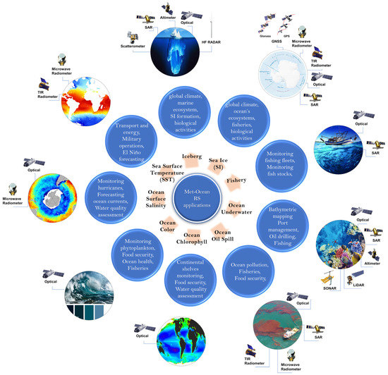
Figure 1.
Overview of the met-ocean applications of RS, which are discussed in this review paper.
2.1. Iceberg
Icebergs are freely floating chunks of freshwater ice calved from marine glaciers, ice shelves, or ice tongues, interacting with the ocean, atmosphere, and cryosphere [5]. With continuous and accelerating global climate change, research on the cryosphere has emerged as a pivotal discipline in climate change studies [6]. Moreover, the cryosphere elements (e.g., icebergs, glaciers, and ice sheets) are recognized as natural climate change indicators due to their sensitivity to small-scale meteorological changes [7]. Recent calving icebergs in both the Arctic and Antarctic have created enormous tabular icebergs, drifting in the open ocean [8,9]. Icebergs, ranging from a few square kilometers up to hundreds of square kilometers, can freely drift in the ocean based on several environmental features, such as ocean currents, waves, wind, and seafloor topography [10]. Iceberg deterioration produces meltwater into the ocean, disrupting and influencing SI formation [11], ocean circulation [12], marine ecosystems [13], SST [14], OSS [14], as well as biological activities [15]. Finally, icebergs can threaten vessel navigation [16] and offshore structures, such as oil and gas platforms [17].
As mentioned, icebergs have many environmental, ecological, and socio-economic impacts. Thus, developing efficient workflows to monitor and track icebergs has been considered a high priority. For instance, the database of iceberg positions was generated to facilitate the navigation of vessels and to conduct research on icebergs and their surroundings [18]. Conventionally, in situ measurements and marine vessels have been employed to obtain accurate information about icebergs [19]. For example, an Aircraft Deployable Ice Observation System (ADIOS) was developed to deploy tracking devices on icebergs from fixed-wing aircraft, enabling the tracking of icebergs through Global Positioning System (GPS) observations [20,21].
Furthermore, other types of sensors, such as terrestrial laser scanners, SONAR, and Autonomous Underwater Vehicle (AUV), have been utilized to collect data about the position, geometry, and morphology of icebergs [22,23]. Although the above-mentioned approaches provide accurate information, they are resource-intensive and logistically arduous in the oceans, especially in remote locations of polar regions [24]. Consequently, it is efficient to employ other RS systems, such as satellites, which can provide broad observations about icebergs through space and time.
Various RS systems have been so far applied to identify and track icebergs [10,25,26,27,28,29,30,31,32,33]. Optical, SAR, scatterometer, altimeter, and HF radar systems have been widely used for iceberg studies. Table 1 summarizes the advantages and disadvantages of each of these systems for iceberg mapping and monitoring. Figure 2 also demonstrates an example of iceberg detection using optical and SAR imagery.

Table 1.
Different RS systems for iceberg studies along with their advantages and disadvantages.
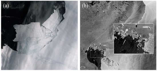
Figure 2.
An example of iceberg in satellite imagery: (a) A 300 square kilometer iceberg spawned from the Pine Island Glacier captured by the Sentinel-2 optical image (ESA, n.d.), and (b) Sentinel-1 SAR data acquired over parts of the Pine Island Glacier and Thwaite Glacier (ESA, n.d.).
2.1.1. Optical
As mentioned in Table 1, optical satellites are considerably beneficial for iceberg mapping and monitoring due to the availability of high-resolution images and the simplicity of iceberg visualization. However, atmospheric conditions, cloud-prone possibility, and the lack of reflected solar radiation, especially in the winters in Arctic regions, are the main limitations of these systems [21].
Generally, floating icebergs have bright sharp boundaries when compared with dark open water, making them easily distinguishable [33]. Furthermore, when other features (i.e., boats, islands, and ships) exist in the imagery, the red and NIR bands could be used to compute the redness index for discriminating these features [27]. For instance, it has been reported that icebergs had redness values between 0.3 and 0.45, while ships were in the range of 0.45 and 0.6 [27].
Both airborne and spaceborne optical satellite images have been extensively applied to detect and monitor icebergs in the Arctic and Antarctic regions [22,33,34]. For instance, A. J. Crawford et al. (2018) investigated the efficiency of aerial photogrammetry for iceberg deterioration estimation. To this end, the Structure-from-Motion (SfM) and deterioration detection threshold algorithms were combined to calculate the masses of two icebergs. The authors recommended developing more sophisticated algorithms based on SfM because it provided promising results for the iceberg’s mass estimation. Additionally, Podgórski and Pętlicki [33] employed very high-resolution Worldview-2 optical images to create a comprehensive calving iceberg inventory (i.e., population, size distribution, and area-volume scaling) of the San Quintin glacier in Chile. They used the multiresolution segmentation algorithm and the Random Forest (RF) classifier to identify icebergs. Various contextual information along with the watershed algorithm were applied to enhance the performance of the proposed approach, enabling the detection of 3184 out of 3212 icebergs. In another study, Heiselberg [27] compared the application of Convolutional Neural Networks (CNN) and Support Vector Machine (SVM) for iceberg-ship classification. The results indicated the higher accuracy of the CNN approach compared to other methods.
Several sophisticated algorithms, including the Cross-correlation in the frequency domain on orientation images [35] and the Normalized Cross-Correlation (NCC) [36], have also been introduced to track and estimate the velocity of drifting icebergs. For example, Liu et al. [28] developed a novel rotation-invariant feature tracking approach to estimate the ice velocity fluctuations from 2004 to 2015 in East Antarctica. To this end, multi-temporal Landsat images were combined, and the obtained results showed an acceptable performance compared to the NCC-based approaches.
2.1.2. SAR
In SAR data, icebergs are the sum of volume and surface scattering mechanisms [37]. The scattering intensity reflects the characteristics of icebergs and, thus, it can be employed to estimate the physical parameters of icebergs (e.g., size, roughness, and freeboard). Due to the scattering properties of icebergs, they appear brighter in comparison with the darker backgrounds of SI and open water. This contrast enabled the researchers to utilize SAR data for iceberg studies. In this regard, great effort was made to employ SAR data for iceberg studies by generating mosaic datasets and developing various Machine Learning (ML) algorithms [25,38,39,40]. For instance, Jezek et al. (1998) utilized over 3000 individual Radasat-1 C-band data, acquired between September and October of 1997, to construct the Antarctic near-coastal zone mosaic dataset. Moreover, Bentes et al. (2016) developed a CNN algorithm to discriminate between ships and icebergs in high-resolution TerraSAR-X images. The CNN algorithm was employed to solve the existing challenges of the algorithm of the constant false alarm rate [41,42]. The achieved high Precision, Recall, and F1-score criteria demonstrated the capability of the CNN algorithm for ship and iceberg discrimination in SAR images. Furthermore, Barbat et al. (2019b) developed an adaptive ML algorithm to improve the automatic detection capability of icebergs in SAR images. The proposed approach was comprised of three concepts of superpixel segmentation, ensemble learning, and incremental learning applied to two SAR mosaic datasets. The low average false positive rate of 2.3 and the high average classification accuracy of 97.5% confirmed the robustness of the proposed method for iceberg detection.
Icebergs are generally observed as brighter than the surrounding backgrounds (i.e., open water) in SAR images. The main challenge of identifying icebergs is when ships have existed in an SAR image. Since some radar signals like L-band can penetrate icebergs there are lower possibilities for corner reflector backscattering returns, while this happens more for ships. In particular, the HH polarization is preferred over VV for only iceberg detection in open water, while the HV polarization proved its higher potential for iceberg-ship discrimination [43].
2.1.3. Scatterometer
As discussed in Part I of this review paper, scatterometers have two main architectures: fan-beam and pencil-beam. Considering their properties, each has its own benefits and limitations for iceberg studies. The fan-beam systems allow for the investigation of the scattering mechanism, while the pencil-beam systems enable narrow azimuthal sampling with broader coverage.
It was also mentioned that σ° could be used to distinguish different targets in the ocean environment. Regarding iceberg studies from RS data, seawater has a lower σ° value than icebergs, which typically can be applied to discriminate between these features. The contrast between seawater and iceberg allows us to locate and monitor icebergs in the oceans. Generally, an iceberg can be efficiently identified by homogenous high σ° values due to the volume scattering of iceberg constituents. For instance, the daily SeaWinds scatterometer data were collected and processed using the resolution-enhancement technique to detect and track large icebergs [44]. The authors only considered large tabular icebergs due to the low resolution of scatterometer data. The icebergs were identified as high-backscattered objects within lower-backscattered surroundings (e.g., SI and seawater) in daily images, enabling real-time positioning of icebergs. The detection and tracking results, which were validated by in situ observation of the National Science Foundation (NSF) ships and high-resolution satellite imagery, demonstrated the high potential of SeaWinds scatterometer data for large iceberg tracking. Additionally, Budge and Long (2018) developed a new consolidated database for the Antarctic icebergs by combining daily positional data from Brigham Young University and weekly tracking data from the National Ice Center (NIC). Currently, Brigham Young University comprises data from several scatterometers (e.g., Advanced SCATterometer (ASCAT) and OceanSat SCATterometer (OSCAT)), and the NIC contains optical and infrared data for the iceberg studies. The size and rotational patterns of the detected icebergs are also estimated from σ° values of scatterometers using the automatic contour estimation method.
2.1.4. Altimeter
Tournadre et al. [45] proved that existing targets on the ocean surface, such as ships and icebergs, were detectable in the thermal noise section of the waveform echoes. These targets can be identified based on radar equations by demining their impact on the waveform echo. Icebergs can significantly affect the altimeter waveform echo and can be detected through their signatures. However, iceberg detection performance by altimeters is negatively affected by the presence of SI, which requires high caution [11]. Considering the Gaussian antenna pattern and altimeter pulses, specific radar equations can be applied to delineate the iceberg signature [46]. The iceberg signature is deterministic and is in parabolic shape in the altimeter waveform echo. Therefore, automatic methods can be developed for their delineation. For instance, Ref. [47] introduced an automatic method based on a convolution product and filtering method to distinguish the parabolic signature of icebergs in the thermal section of altimeter waveform echo. This method was then applied to estimate the minimum height of approximately 8000 icebergs using one-year Jason data. Furthermore, Ref. [48] created a database (e.g., position, size, and volume) of small icebergs using archives of nine altimeters between 1992 and 2014. Intercalibrated altimetric data were merged to obtain reliable monthly iceberg volumes. Finally, the correlation between global small and large iceberg volumes revealed that the smaller icebergs were dominantly generated by the disruption of larger ones. Furthermore, Ref. [49] implemented eight ML algorithms to discriminate icebergs and ships using Jason-2 satellite altimetry data. The reference samples were generated using ENVISAT-ASAR images, and the results indicated the superiority of the SVM algorithm for iceberg-ship discrimination.
2.1.5. HF Radar
Although HF radar has been mostly employed for the RS of the ocean surface, it also has iceberg detection capability. However, the detection of icebergs in the Doppler spectrum received from the ocean surface might be challenging. This is because the backscattered fields from the ocean surface spread over a wide range of frequencies, particularly close to zero Doppler, where the iceberg returns occur [50]. In other words, the clutter can mask the iceberg return because both of them appear in a narrow frequency band around zero Doppler. In this regard, Ref. [51] proposed an analytical method based on the generalized functions approach [52,53,54] to estimate the scattered field for mixed paths with discontinuities, which is an extension of [55] for the analysis of scattered fields over layered media. Moreover, Walsh and Srivastava [56] developed the radar cross-section of icebergs with arbitrary size and shape in the presence of a vertical dipole antenna using the presented methods in [51,55]. Ref. [50] also compared the iceberg-measured spectrum parameters with modeled spectrum to show the validity of their developments in [56]. An experiment was conducted using an HF radar operating at 25.40 MHz between July and August 1984 at Byron Bay, Labrador, to test the accuracy of the proposed method.
2.1.6. Summary and Future Direction
Based on both the advantages and disadvantages of RS systems for iceberg mapping and monitoring, several strategies can be considered in future research to enhance iceberg studies. In this regard, synergistic use of RS systems could help in obtaining results with a higher confidence [10]. Additionally, multi-source RS systems resolve the revisit time limitation and provide further opportunities for iceberg detection [28]. Furthermore, the development of RS systems with more advanced specifications (e.g., higher spatial and temporal resolutions) would benefit iceberg studies [29]. For example, developing SAR systems with higher penetration capability (e.g., L-band SAR systems) can considerably facilitate iceberg detection and relevant parameter estimation [29]. Finally, the availability of a huge volume of RS data requires more sophisticated data mining and processing algorithms (e.g., Deep Learning (DL)) and big data processing platforms (e.g., Google Earth Engine (GEE)) to exploit the full potential of RS data for iceberg studies [30,31,32].
2.2. Sea Ice (SI)
SI is formed when the surface water of the ocean freezes. The main difference between SI and glaciers or icebergs is that SI forms from salty ocean water, while glaciers and icebergs form from fresh water and snow [57]. Generally, SI forms, grows, and melts exclusively in the ocean [57]. Although SI can cover up to about 30 million square kilometers of the Earth’s surface [58], many people might never directly encounter SI in their lives because SI is found primarily in the Arctic and Antarctic regions [57,58]. SI has direct and indirect effects on the climate, wildlife, and many human activities. Because of its bright surface, SI has a high surface albedo and reflects a significant portion of the sunlight into space because of its bright surface. The high surface albedo decreases the solar energy absorbed by SI and helps to keep the temperature of the polar regions low [59]. The warmer climate in the polar regions melts SI and decreases the bright surfaces’ ability to reflect the received sunlight. Consequently, even a minor SI loss in the polar regions can lead to a global cycle of warming and melting [59].
Moreover, SI affects the thermohaline circulation by changing the water temperature, water salinity, and salt concentration [60]. SI also influences global atmospheric circulation by affecting the heat exchange between the ocean and the atmosphere [61]. Additionally, many animals that live in the Arctic and Antarctic, such as polar bears, penguins, and seals, depend on and are heavily affected by SI and its changes [62]. SI is also very crucial for human activities in the Arctic and Antarctic. For instance, indigenous people living in the Arctic depend on SI-covered areas for transportation, fishing, and hunting [63]. Finally, SI mapping and monitoring are essential for many industrial operations, including oil rigs, factories, safe ship navigation, and scientific research in polar regions [63,64].
Despite its crucial role, gathering in situ data for SI studies is very difficult due to their remote locations, extreme climate, and changing nature. Scientists have previously used ships, submarines, buoys, and field camps to gather data for SI monitoring over relatively small regions [58]. These methods are costly and labor-intensive. However, RS provides various types of information from remote locations in broad areas and with suitable spatial and temporal resolutions. Consequently, RS techniques have become the primary data gathering methods for SI studies [65]. Various characteristics and physical parameters of SI, including extent [66,67,68], thickness [69,70], drift and motion [6], lead [71], temperature [72], type [73], age [74], and snow cover [75] can be effectively derived from RS datasets.
The reflected, emitted, or backscattered electromagnetic energy in the visible, Near Infrared (NIR), Thermal Infrared (TIR), and microwave parts of the electromagnetic spectrum can be measured by different RS systems to study SI. Different characteristics of SI (e.g., thickness, temperature, type, and age) can affect the electromagnetic wave received by RS systems and, thus, can be measured by these systems. Based on these characteristics, many studies have applied RS data to study SI [76,77,78,79,80,81,82,83,84,85]. Moreover, imaging (e.g., geometry, imaging season, and weather conditions) and sensor (e.g., frequency, spatial resolution, and polarization) properties can affect electromagnetic energy and should be considered in SI mapping and monitoring using RS systems [76]. Table 2 summarizes different types of RS systems along with their advantages and limitations for SI studies. More details of the most commonly used RS systems for SI studies (i.e., optical, TIR radiometers, microwave radiometers, SAR, scatterometer, and altimeter) are also provided in the following subsections.
Table 2.
Different RS systems for SI studies along with their advantages and disadvantages.
2.2.1. Optical
Although the primary focus of SI remote sensing has been on microwave RS systems, especially active sensors, optical imagery, which measures the solar radiation reflectance from the earth, has also provided valuable information for SI studies [66,73]. SI usually appears brighter than the surrounding water in the visible bands of the optical satellite images due to the high surface albedo. Many researchers considered this feature and applied a global or local threshold to distinguish SI from ocean water in optical imagery [66,69]. Additionally, histogram analysis based on the higher reflectance of the SI has been used for SI classification in optical images [73]. Moreover, texture analysis and image segmentation algorithms, considering differences in statistical texture features between ice and water, have been utilized through various texture analysis methods (e.g., Gray Level Co-occurrence Matrix (GLCM)) for the SI extent and outer edge detection [67].
Many multispectral satellites have been used for SI studies. Some of the most frequently used spaceborne optical systems for SI studies are the Moderate Resolution Imaging Spectroradiometer (MODIS), Advanced Very High-Resolution Radiometer (AVHRR), Visible/Infrared Imager Radiometer Suite (VIIRS), Landsat, and Sentinel-2. For instance, Ref. [67] utilized the GLCM texture analysis for SI detection using MODIS multispectral images over the Bohai Sea. The prominent differences between the SI and water statistical texture features were used in this study, along with a texture segmentation method for mapping SI extent and its outer edge. Textural analysis resolved the spectral confusion and SI misassignment due to the suspended sediment presence, which is problematic in Bohai SI detection through conventional thresholding methods. The 30 m spatial resolution imagery of HJ1B-CCD was also used for visual validation and statistical accuracy assessment by calculating the confusion matrix. It was reported that the difficulty of cloud separation from SI due to their similar textural features was the main limitation of the proposed method.
Despite the feasibility of SI monitoring through optical imagery, multiple limitations restrict the practical application of visible, NIR, and Shortwave Infrared (SWIR) spectral bands for SI monitoring. For example, since visible and infrared radiations can be reflected and emitted from clouds, optical systems cannot collect data under clouds, which is very common in polar regions. Additionally, since the reflection of the sunlight is an essential prerequisite for imagery in the visible, NIR, and SWIR bands, these sensors can only collect daytime data, which is problematic in the dark seasons of the polar regions. Finally, other natural phenomena, such as the suspended sediment or the clouds, have similar spectral characteristics with SI making it difficult to distinguish them in optical imagery [58,67].
2.2.2. TIR Radiometer
The images acquired by TIR radiometers, which can be interpreted as an indication of the heat emitted by the surface, have been utilized for SI studies, including SI condition monitoring [86], SI surface temperature estimation [72], SI thickness modeling [70], and SI lead detection [71]. Furthermore, thermal bands have proved useful for other applications related to SI, such as wildlife monitoring in polar regions [87]. Among various TIR systems, MODIS and AVHRR instruments have been frequently used for SI monitoring. Although the application of TIR images, especially for SI thickness retrieval, has also been proved in multiple studies [88,89], the major problem is still the cloud cover in TIR images [90]. Furthermore, the temperature of the newly formed thin SI is very close to the freezing water, which makes it difficult to be distinguished from the surrounding water. During summer, the melting surface of SI also has a temperature close to the freezing point and would be very similar to the surrounding water that is also in the freezing point [58,67].
2.2.3. Microwave Radiometer
Due to the higher microwave radiation emitted by SI compared to clouds, microwave radiometers can gather data during day and night and regardless of the cloud condition. This feature makes microwave radiometers suitable for SI studies. The most important parameter determining the amount of microwave radiation emission from SI are its physical properties, such as atomic composition and crystalline structure [91]. Among different microwave radiometers, the Special Sensor Microwave/Imager (SSM/I) and the Special Sensor Microwave Imager Sounder (SSMIS) are the most frequently used radiometers for SI mapping and monitoring [92]. Moreover, the Scanning Multichannel Microwave Radiometer (SMMR), Advanced Microwave Scanning Radiometer for EOS (AMSR-E), and Advanced Microwave Scanning Radiometer 2 (AMSR2) have provided valuable data for SI studies. For instance, Ref. [92] retrieved SI concentration from microwave radiometer data. The National Aeronautics and Space Administration (NASA) Team algorithm and the artist SI algorithm were utilized in this study to retrieve SI concentration. The developed algorithm was applied to the brightness temperatures measured by the SSM/I instrument in different channels. Furthermore, the Wide Swath Mode ASAR images with 150 m × 150 m spatial resolution and MODIS band-1 images with 250 m × 250 m spatial resolution were used for the evaluation.
The main limitation of microwave radiometers is their relatively coarse spatial resolution due to the low emitted microwave radiation. The coarse spatial resolution restricts many SI applications, such as SI lead detection, and increases the mixed-pixels problem [92,93].
2.2.4. SAR
Generally, a newly formed thin ice would have a smooth surface which causes specular reflectance and appears very dark in SAR images. The specular reflectance makes it challenging to distinguish thin and new SI on a calm water surface as a specular reflector [58,94]. When SI is covered with moist snow, it usually has volume or composite scattering, making such areas appear bright in SAR images [94]. The aged SI can also cause volume scattering. Moreover, the morphology of the SI can change due to temperature fluctuations and SI movement [94]. These changes would roughen the SI surface and create small pressure ridges. Therefore, aged SI would appear brighter in SAR images because of the rough surface [58,94].
The imaging frequency and polarization of SAR systems are important for SI mapping. For example, Figure 3 illustrates various properties of SI in C-, L-, and P-bands SAR images [94]. As is clear, C-band was a better discriminator for new and aged SI. Additionally, the penetration of the microwave radiation in L- and P-band would complicate the interpretation of SI scattering characteristics, especially for new and aged SI discrimination. However, L-band was generally reported to be a better demonstrator of the pressure ridges of the SI [94]. In terms of polarization types, the Horizontal transmit and Horizontal receive (HH) polarization is generally the preferred polarization for discriminating SI from ocean water because it is less sensitive to water roughness than the Vertical transmit and Vertical receive (VV) polarization [94]. For example, Ref. [95] extracted 12 different polarimetric features from the HH-VV dual polarization TerraSAR-X images and trained an Artificial Neural Network (ANN) for pixel-wise SI type classification. A comprehensive statistical analysis of the correlation between the extracted polarimetric features and their relevance for SI classification was conducted in this study. It was observed that the features purely based on the covariance matrix were more informative for SI classification than the features involving eigen decomposition of the coherency matrix. The in situ data acquired during the N-ICE2015 field campaign was also used for validation. The percentages of in situ samples of each SI class that were assigned to the respective SI type by the classifier were computed to assess the stability of the classification procedure. Over 90% stability for almost all SI types indicated that the approach was consistent and stable.
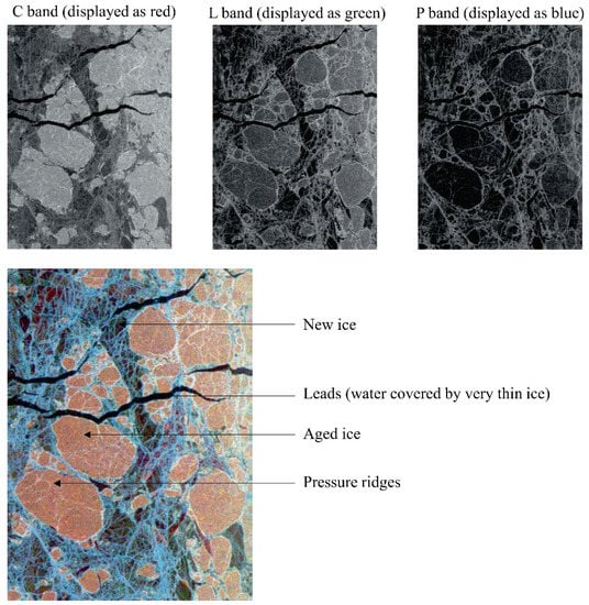
Figure 3.
Different properties of SI in different channels of SAR images [94].
So far, many SAR satellites have so far provided valuable data for SI mapping and monitoring. For example, RADARSAT-1 and -2, Sentinel-1, ENVironmental SATellite (ENVISAT), TerraSAR-X, and Advanced Land Observing Satellite (ALOS) satellites have been extensively used for SI studies.
2.2.5. Scatterometer
Although scatterometers are mainly designed for OSW measurements, they have also proved to be useful for SI studies [96,97]. Scatterometers directly measure the Normalized Radar Cross Section (NRCS), from which the wind parameters can be extracted. The measured NRCS data can also be utilized for other applications, including SI studies [96]. Despite their coarser spatial resolution, scatterometers can provide daily data from polar regions to study SI, which makes them very useful for global SI monitoring [85]. Among various microwave scatterometers, the Ku-band NASA scatterometer (NSCAT) onboard the Advanced Earth Observing Satellite (ADEOS) platform, the Ku-band SeaWinds scatterometer instrument of the QuikSCAT, OSCAT onboard the OceanSat-2, and C-band ASCAT carried by MetOp-A are the most commonly used spaceborne scatterometers for SI studies.
2.2.6. Altimeter
Altimeters are mainly used to determine the topography of the SI surface, which can be used to calculate SI thickness [85]. The calculated SI thickness from altimetry data is invaluable for the SI volume change monitoring [85]. Cryosat, the European Space Agency (ESA) mission, launched in April 2010, is specifically designed to provide polar ice data, including SI altimetry. Additionally, other altimetry missions, such as Joint Altimetry Satellite Oceanography Network (JASON) satellites, NASA Radar Altimeter (NRA) on board of the TOPEX-Poseidon, and Synthetic Aperture Radar Altimeter (SRAL) on Sentinel-3 missions, have provided altimetry data for SI studies. Finally, laser altimeter instruments, which use visible pulses for altimetry measurements, have also been employed for SI studies. The data acquired by the Ice, Cloud, and land Elevation Satellite (ICESat-1) and ICESat-2 are the most popular laser altimetry data for SI studies [85].
In terms of ML algorithms, the SVM algorithm has shown a high potential for SI classification [81]. Additionally, rule-based ML models, including the decision tree and RF algorithms, have been utilized for deriving melt pond statistics and detection [82], as well as for SI thickness estimation and leads detection [83]. Dumitru et al. [84] also implemented an automated processing chain using content-based ML algorithms to analyze and interpret the specific ice-related parameters using high-resolution SAR images.
2.2.7. Summary and Future Direction
Despite the significant advances in SI monitoring using RS techniques, there are still several challenges. For instance, due to the fast-changing nature and seasonal changes of SI conditions, RS data with a higher temporal resolution is required for up-to-date information on SI. The launch of recent satellites has an important role in alleviating this issue. Furthermore, the snow cover affects the reflected or backscattered signal from the SI surface and complicates the detection and classification of various SI types, as well as the estimation of their physical parameters [85]. These issues might be resolved using multi-sensor observations. Additionally, the snow cover causes uncertainty in the SI thickness measurements using the altimetry sensors, which could be mitigated by the combined use of laser and microwave altimeters [85]. Moreover, despite the penetration capability of microwave systems into the cloud, the existence of thick clouds, which is common in the Arctic and Antarctic, may affect the microwave signal and results in ambiguous information about SI [29,85]. Another challenge in SI monitoring using RS is the heterogeneity and incompatibility of different measurements. Many SI studies have been carried out by independent teams with varying standards and formats, which is problematic for comparing these measurements and acquiring long-term SI information. In the future, a standardized format for SI measurements could resolve this issue [29].
The portion of SI studies that have utilized microwave RS, especially SAR data, has been increased in recent years. This is because of the remarkable advantages of this data, recent advances in SAR data processing techniques, and the availability of SAR images. However, multi-source studies are necessary to achieve all-weather, real-time, and large-scale SI monitoring programs. Moreover, using multi-platform measurements (satellites, drones, ships, and ground-based stations) is also important to study different aspects of SI. Therefore, multi-source multi-platform SI monitoring will be of immense importance in future studies.
Developing more advanced ML models for SI study will be another future direction in this field. Different ML and data processing algorithms have been evaluated for SI studies using various RS datasets. Like many other RS applications, DL methods have proved to be very beneficial for SI studies [77,78,79]. However, DL models require a very large number of training data and are computationally expensive [80]. Consequently, it is sometimes more reasonable to utilize other less costly ML algorithms.
Finally, different oceanographic parameters are not independent, and each parameter affects and gets affected by the other parameters. So far, a few studies have been conducted to relate SI with other oceanographic parameters, Thus, multi-phenomena studies and considering the effects of the other parameters on SI should be investigated further in future studies.
2.3. Sea Surface Temprature (SST)
SST is one of the most important oceanic variables for the global climate system and has been widely utilized to forecast and monitor long-term climate changes [98,99,100]. Moreover, the fluctuating flux of dormant and sensible heat from the ocean affects the atmosphere. Thus, SST is often used as a critical variable to study the atmosphere-ocean interaction at different scales [98,99,101,102,103]. Furthermore, SST measurements are widely used in various operational applications, such as civilian and military maritime operations [104], validation of atmospheric models [105], estimation and prediction of coral bleaching [106], human health [107], food security and environmental policy [108], transport and energy [109,110], tourism [111], tracking marine life [112,113], studding the El Niño and La Niña events [114], and commercial fisheries management [115].
SST measurements are negatively affected by variability and complexity of temperature over ocean surface layers due to various factors, such as air–sea fluxes of heat, moisture and momentum, and ocean turbulence [98]. To address the challenges of variation of sea skin temperature, the Group for High Resolution Sea Surface Temperature (GHRSST), as an open international science team, classified SST into five categories [116,117,118,119]: (1) interface SST(SSTint), which is the temperature at the exact air–sea interface on microscopic scales and cannot be measured using current technologies [119]; (2) skin SST (SSTskin), which is the temperature retrieved by an TIR radiometers (wavelength = 3.7–12 μm) within the conductive diffusion-dominated sub-layer with the depth of approximately 10–20 μm; (3) sub-skin SST (SSTsub-skin), which is the temperature at the base of the conductive laminar sub-layer of the ocean surface measured by microwave radiometers (frequency = 6–10 GHz); (4) SST at depth (SSTdepth or SSTZ ), which is defined as the temperature at the bottom of the SSTsub-skin, and is measured by drifters, autonomous/non-autonomous profiling floats, or deep thermistor chains at different depths; (5) foundation temperature (SSTfnd), which is the temperature at the first time of the day and is independent from diurnal temperature variability and is only measured by in situ contact thermometry at the depths of approximately 1–5 m.
Figure 4 demonstrates a schematic diagram of the day and night temperature profiles of the ocean near-surface layer for each SST definition. Based on this figure, SST measurements are affected by the main heat transport processes and time scales [119]. During the day, most of the incoming solar radiation is entered into the near-surface ocean (5 m depth), leading to the formation of thermal stratification (layers of different temperatures) in the ocean. This effect is exacerbated by the light winds (low wind speeds) [98,120,121,122]. On the other hand, the water column gradually cools from the surface during the night [120]. This heating and cooling cycle creates a diurnal cycle in SST, which is very important in improving the ocean-atmosphere models [120,122].
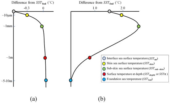
Figure 4.
Near-surface oceanic temperature profiles for different types of SSTs at (a) nighttime and (b) daytime (adopted from the Group for High Resolution Sea Surface Temperature (GHRSST)).
SST can be measured by deploying temperature sensors on different instruments, such as in situ moored and drifting buoys, ships (with a thermometer into a bucket of seawater), and offshore platforms, as well as airborne and spaceborne RS systems [99]. Since 1970, by deploying the Visible and Thermal Infrared Radiometers (VTIR) on geostationary satellites, using SST measurements derived from RS data has become routine [98]. In this section, SST measurements from spaceborne RS systems are only discussed. The satellite-based SST is determined by estimating the thermal emission of electromagnetic radiation from the sea surface using radiometers, which can be expressed by the Planck’s Function (Equation (1)) [123,124].
where Bλ refers to the Brightness Temperatures (BT); T is the sea surface at absolute temperature; h is Planck’s constant; c is the speed of light (in the vacuum); k is the Boltzmann’s constant; and λ is the wavelength [124]. According to Planck’s Equation, radiance at a known wavelength should be measured to determine the emitting temperature from the sea surface [98].
Two types of spaceborne RS systems, both of which are passive systems, can be mainly used for SST measurement: TIR and microwave radiometers. The TIR spaceborne systems are onboarded on the Low-Earth Orbiters (LEO) and Geostationary (GEO) satellites, while the microwave radiometers are onboarded on the LEO orbiters. The advantages and disadvantages of each system for SST estimation are provided in Table 3. Moreover, the main satellites to estimate SST are demonstrated in Figure 5.
Table 3.
Different RS systems for SST estimation along with their advantages and disadvantages.
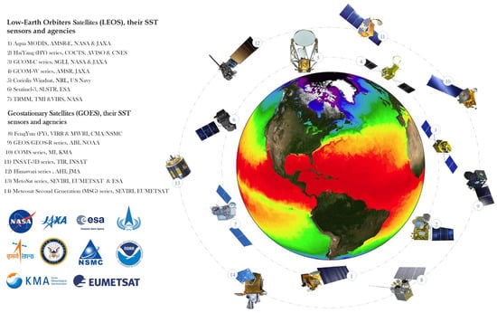
Figure 5.
The main satellites for SST measurements.
2.3.1. TIR Radiometer
TIR radiation does not penetrate through clouds. Even in cloud-free conditions, the atmosphere scattering and absorption can negatively affect TIR radiation due to haze and aerosols [125,126,127]. The transmissivity of the clear-sky atmosphere in the TIR range of the electromagnetic spectrum depends on the wavelength and absorptions of atmospheric gases [124]. Consequently, the TIR wavelength intervals in an RS system should be carefully determined based on the atmospheric window where the atmosphere is more transparent [98]. The TIR radiometers measure SST within two atmospheric windows at λ = 3.5–4.1 μm and λ = 9.5–12.5 μm [128]. However, measurements at the λ = 9.5–12.5 μm window are negatively affected by solar effects, making them usable only at nighttime [98].
The presence of clouds is one of the most important challenges in measuring SST using Equation (1), which requires an accurate scheme for removing cloud-contaminated and weather-contaminated pixels [98,129,130,131]. Identifying the clear sky pixels is a fundamental step for achieving an accurate time-series SST estimation [131]. In this regard, many algorithms have been proposed for cloud screening in TIR measurements, including BT minima, binary tests in a decision tree based on BT uniformity, and comparisons with lower-resolution gap-free reference fields [130]. However, these methods depend on the selected threshold values, resulting in potential errors in SST estimation at high latitudes and near ocean thermal fronts at semi-transparent clouds [98,129,132].
To address these limitations, a Bayesian probabilistic approach was proposed in [133] for cloud screening of TIR imagery, which was widely used for operational SST estimation in several satellite missions, such as the Advanced Along-Track Scanning Radiometer (AATSR) [134], the Geostationary Operational Environmental Satellite (GOES) [135], and the Japanese geostationary meteorological Himawari-8 satellite [136]. Moreover, alternating decision tree [137,138] methods were identified to improve the performance of the decision-tree approaches in cloud screening, where instead of trial-and-error methods, ML algorithms are applied to determine threshold values and their weights.
After cloud screening, SST can be mainly obtained using the Single-Channel (SC) and Multi-Channel (MC) approaches. Measuring SST using the SC method requires the sea surface emissivity and the atmospheric profiles, which can be obtained using the following equation [128,139]:
where , , and refer to the sensor spectral radiance, the downward radiance of atmosphere, and Top Of Atmosphere (TOA) spectral radiance, respectively; and are the atmospheric transmittance and the emissivity of the sea surface, respectively. The is computed using the geometric-optics models [140,141] of the sea surface in the TIR atmospheric windows and the rest of the parameters are computed from the Radiative Transfer (RT) models. SST estimation using the SC method is negatively affected by uncertainties from the profile fed into the model and limitations in modeling water vapor absorption [128]. In fact, these methods can only be used for SST estimation when accurate atmospheric profiles are available. To cope with these uncertainties, MC methods that use the differential BTs measured in the two or more than two channels were proposed. Equation (3) provides the general formulation for an MC algorithm [98,124]:
in which and are the BTs measured in the two channels; c is an offset; and γ is the water vapor absorption coefficient. The MC methods have a high potential for SST estimation from all TIR radiometers with at least two thermal channels, and there is no need for accurate atmospheric profiles [142]. The coefficients in Equation (3) can be derived by regression analysis or RT simulations [98,124,129].
Since MC algorithms are not sufficiently accurate to represent the water vapor effects [98,129], a group of other algorithms, called the nonlinear SST algorithms [143,144] have been developed. These equations are mainly based on the BT values of the channels at the atmospheric windows (i.e., λ = 3.5–4.1 μm and λ = 9.5–12.5 μm) with correction terms of the effects of atmospheric moisture and satellite zenith angles [131]. Moreover, depending on the selected atmospheric windows, these equations can be divided into three categories of dual window (at λ = 3.7 and λ = 11 μm), split window (at λ = 11 and λ = 12 μm), and triple window (at λ = 3.7, λ = 11 μm, and λ = 12 μm) [129,145].
TIR radiometers onboarded LEO can produce global SSTs at a medium spatial resolution [99]. The number of thermal bands and the spatial resolution are the most important characteristics of the TIR radiometry for SST estimation. For example, the hyperspectral TIR radiometers with several narrow spectral bands are very useful for SST estimation [98]. The Atmospheric Infrared Sounder (AIRS) [146] deployed on the NASA satellite Aqua, and Infrared Atmospheric Sounding Interferometer (IASI) on the three Metopolar-orbiting satellites of the European Organization for the Exploitation of Meteorological Satellites (EUMETSAT) [147] are the examples of the hyperspectral TIR sensors which have been used for SST estimation. For example, Figure 6 demonstrates SST products generated from ASTER and MODIS around the Sendai Bay. As is clear, the thermal variations of coastal waters in Sendai Bay are more evident in the ASTER SST image compared to that of the MODIS, indicating the potential of ASTER data to produce high-resolution SST maps in the coastal areas.
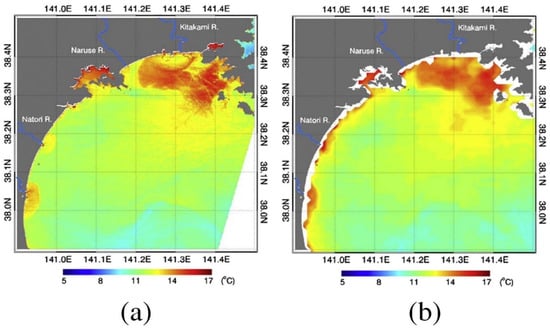
Figure 6.
SST maps at 01 UT on 2 May 2003 generated from (a) ASTER image with 90 m spatial resolution and (b) MODIS data with 1 km spatial resolution [100].
Landsat, ASTER, and MODIS are among the most important LEO TIR radiometers for SST estimation. For example, Landsat-8 has two TIR channels (λ = 10.3–11.3 μm, and λ = 11.5–12.5 μm) with a spatial resolution of 100 m, which are very helpful for estimating SST in coastal waters [98]. Moreover, ASTER onboard the Terra satellite acquires images with 14 spectral channels, five of which are TIR channels, with a spatial resolution of 90 m. These datasets are also valuable for accurate SST estimation, especially for coastal areas [98,100]. MODIS data with four TIR channels (channels 29, 30, 31, and 32) has also been widely used to estimate SST. The ECOsystem Spaceborne Thermal Radiometer Experiment on Space Station (ECOSTRESS) is also another source to derive high-resolution SST products using five spectral bands (λ = 8.29, 8.78, 9.20, 10.49, 12.09 μm) with the spatial resolution of 38 m × 68 m [98]. The LEO TIR systems have been widely utilized for SST retrieval. For example, Matsuoka et al. [100] developed a statistical algorithm for high-resolution SST retrieval from the TIR channels of ASTER data in the coastal waters of Sendai Bay, Japan. The results indicated that ASTER SST products were independent of the satellite zenith angle. Moreover, Cavalli (2017) [148] proposed an accurate technique for SST estimation from MODIS data. Their method was based on the incorporation of column water vapor value and the effect of total suspended particulate matter concentration on Sea Surface Emissivity (SSE) values. The results indicated that the proposed approach accomplished a decrease in SST estimation error in coastal waters by incorporating the effect of total suspended particulate matter in the estimation of SSE. Finally, Koner (2020) [149] proposed a daytime split-window technique for SST retrieval from MODIS data by incorporating the mid-wave channel/s. The results showed that the proposed method was superior to the physical deterministic SST retrieval scheme.
Although the GEO TIR satellite images have coarser spatial resolution compared to the LEO satellites, they provide SST data with higher temporal resolutions (e.g., every 15 min) over a large portion of the globe [1,4,99,150]. Thus, the corresponding SST products are widely used in clear-sky masking to describe the SST diurnal variations [99]. The GEO TIR radiometers provide approximately global SST measurements, missing only high latitudes [99,150,151]. For example, the field of view of GOES-16 (in the East position), Meteosat-8 (over the Indian Ocean), and Meteosat-11 (over the Atlantic Ocean), which are processed by the OSI SAF [152] are demonstrated in Figure 7.
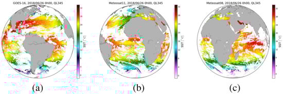
Figure 7.
SST maps from (a) GEOS-16, (b) Meteosat-11, and (c) Meteosat-18 [151].
2.3.2. Microwave Radiometer
The cloud penetrating capability of microwave radiometers enables them to provide SST data regardless of the cloud cover and atmospheric aerosols [98,99,153]. At long wavelengths, where hc ≪ λkT, the spectral radiance can be formulated using the Rayleigh-Jean Law (Equation (4)) instead of Planck’s Function [1]:
where
in which T is the thermodynamic temperature; and ε denotes emissivity. When radiation passes through the atmosphere, some portions of it are absorbed, scattered, and emitted. Consequently, the measured BT by radiometers can be obtained based on the following equation [98]:
where , , and are the temperatures of the surface, upward atmosphere, downward atmosphere, and space, respectively. The RT models and statistical algorithms are typically employed for deriving SST from microwave radiometer measurements [98]. These models require environmental data (e.g., SST, atmospheric profiles, and wind speed/direction) and radiometer information (e.g., frequency, polarization, azimuth, and incidence angle) for modeling the TOA BTs [98]. The performance of such algorithms is dramatically reduced by the presence of instrument calibration errors and inaccurate environmental data [154]. However, the implementation of the statistical algorithms is much simpler, and calibration errors can be compensated in these methods [155]. Generally, the predicted SST by both techniques is negatively affected by variations in wind speed and foam coverage [153].
Different microwave radiometers have been launched and employed for SST estimation. AMSR2, AMSR-E, SMMR, Windsat, GPM Microwave Imager (GMI), and TRMM Microwave Imager (TMI) are well-known microwave radiometers for SST estimation. The Remote Sensing Systems (RSS) organization generates the SST products provided on a daily, 3-days, weekly, and monthly basis using the TMI, AMSR-E, WindSat, AMSR2, and GMI datasets.
2.3.3. Summary and Future Direction
The availability of more RS observations and advanced SST retrieval algorithms in recent years has facilitated generating high-quality SST products. However, there are still several challenges and opportunities in SST estimation that need to be addressed in the future. For example, although DL algorithms have exhibited better performance for deriving accurate SST products, they are data-hungry models and not robust against variation in data distributions, resulting in a reduction in their generality in SST estimation [156]. To address this issue, several rule-based information can be added to the learning process of DL algorithms to improve their robustness. Transfer learning or semi-supervised learning could also improve the efficiency of DL algorithms in SST estimation [157,158]. Moreover, since many DL algorithms have been developed in recent years, comparing their performance in SST prediction can show their potential benefits and extend novel research ideas. Of course, such studies require different local and global datasets, which must be prepared in collaboration with space agencies, oceanographic institutes, universities, and research institutes.
Extensive advancement has been made in large-scale SST mapping with TIR and microwave radiometers. However, the corresponding products still need to have better spatial and temporal resolutions. Estimating precise SST from satellite observation in the Polar regions (high latitude regions) has remained a challenge due to different factors, such as atmospheric conditions. More advanced SST algorithms are required for producing accurate SST products in these regions. Moreover, Unmanned Aerial Vehicles (UAVs), which are equipped with thermal sensors have emerged as a feasible and low-cost option for retrieving SST and temperature profiles from Polar regions [159].
High-resolution SST products are one of the most critical factors for generating accurate and stable climate models. As mentioned before, such products can be retrieved from UAV observations, but typically on a local scale. In this case, advanced image/signal processing algorithms are required to produce global high-resolution SST products from low-resolution RS observations, which are nothing but super-resolution algorithms. Although several DL-based super-resolution methods have recently been developed to generate high-resolution SST maps [158], more research work is required for this purpose.
2.4. Ocean Surface Salinity (OSS)
OSS is defined as the amount of dissolved salt in ocean water, which affects the electrical conductivity of water [160], and is measured in Practical Salinity Units (PSU). The average ocean salinity is about 35 PSU, meaning that there are 35 g of salt in each liter of ocean water [160]. Since salinity is defined as the salt density in a water solution, it is affected by ecological processes which alter the amount of water or salt, such as ice formation or melting, evaporation or precipitation that can change the amount of fresh water in the solution, and river runoffs which enter salty matters into the ocean [161]. Moreover, global ocean circulations in both horizontal and vertical directions change the amount of OSS [160].
OSS is an important parameter for oceanographic applications, such as ocean circulations and biogeochemical processes, and is widely used in ocean forecasting models [162]. OSS is also an important variable in understanding the amount of terrestrial substance delivered into the ocean [163], water density, carbonate chemistry near coasts and deep ocean waters, water acidification [164], optical properties, and algal blooms in coastal regions [163]. Additionally, a better understanding of OSS provides more profound knowledge of coastal water quality and hazards, marine pollution, ocean-atmosphere interactions [165], river discharge into the oceans and river-influenced regions [166]. Moreover, OSS is a key parameter in monitoring hurricanes, El Nino and La Nina forecasting, predicting terrestrial floods and droughts, understanding rainfall over the oceans, and forecasting ocean circulations [167].
In situ ocean salinity measurements are mostly collected by the Array for Real-time Geostrophic Oceanography (ARGO) floats, moored buoys, ocean drifters, surface gliders, Thermo-Salino-Graph sensors, research vessels, marine mammals, and XCTD profilers [161,168,169,170,171]. Continuous monitoring of global OSS was a difficult task until 2009 due to the low density of these in situ measurements and unreliable global models. However, launching the first RS system capable of OSS measurements in 2009 (i.e., Soil Moisture and Ocean Salinity (SMOS) microwave radiometer) brought new opportunities for various oceanographic applications. It should be noted that although in situ measurements do not suffice for mapping OSS [171], mainly because they are the only representative of one specific geographical point [172], they are usually required to calibrate, train, and validate the RS models. To this end, various physical parameters of the ocean, such as temperature, conductivity, and depth which provide salinity based on the electrical conductivity of the water can be used [160]. Moreover, in situ instruments are usually collated from lower than 1 m depth while satellite-based OSS values refer to a few centimeters on top of the ocean [170]. Therefore, this difference should be considered when in situ and RS data are jointly utilized in oceanographic models.
Two types of RS systems can be mainly used for OSS estimation: optical and microwave radiometers operating in L-band. Table 4 provides these RS techniques along with their advantages and disadvantages. More information about the applications of each system for OSS estimation is provided in the following two subsections.
Table 4.
Different RS systems for OSS estimation along with their advantages and disadvantages.
2.4.1. Optical
The first group of spaceborne OSS products is based on reflectance measurements from optical satellites. The corresponding algorithms are based on a direct relationship between OSS and another ocean parameter, such as OC [160]. The Colored Dissolved Organic Matter (CDOM) [160], single-band reflectance from MODIS [173], SeaWiFS [163], Geostationary Ocean Color Imager (GOCI) [174], Landsat [175], and Sentinel-2 [176], as well as band ratios and band combinations from these satellites, are different methods to empirically estimate OSS from reflectance data.
Both statistical and ML models have been so far applied to derive OSS using optical imagery. For example, Reul et al. (2020) developed a regression model to estimate OSS from CDOM values in coastal areas to estimate the extent of the problem of saline waters. Additionally, Yu (2020) [177] used seven years of cloud-free MODIS and in situ data along with an ANN model to fill the gap of lacking nearshore OSS measurements in the Northern Gulf of Mexico coast. Finally, West et al. [163] proposed a method to generate NRT OSS maps with a resolution of 1 km from MODIS and SeaWiFS data using an ANN model.
2.4.2. Microwave Radiometer
Microwave radiometers can estimate OSS by measuring ocean BT [161]. The dielectric constant in open water is determined using microwave frequency and electrical conductivity. The ocean surface emissivity is a function of the dielectric constant and the state of the surface roughness. In principle, OSS can be estimated from BT observations [178]. The emissivity is the linking quantity between BT and OSS [160] and depends on multiple parameters.
Multiple factors affect the spaceborne BT measurements from microwave radiometers, consequently decreasing the accuracy of the retrieved OSS. For instance, land contamination in large ground pixels (pixel sizes of about ~50 km) and antenna orientation (due to the existence of side lobes) decrease the OSS accuracy [171]. Furthermore, SI contamination occurring in high latitudes could affect OSS estimation [162]. On the other hand, BT values derived from microwave radiometers are less accurate in cold waters (polar regions) due to the reduced sensitivity of L-band measurements [162]. Moreover, several variables, such as Radio Frequency Interferences (RFI), solar and galactic radiations, ionosphere Faraday rotation, surface roughness, and atmospheric effects should be precisely modeled to obtain an accurate OSS product using microwave radiometer data [161]. It is also worth noting that some error patterns have not been fully modeled. For instance, SMOS is affected by seasonal biases, differences between ascending and descending passes, and some systematic sources of RFI [179]. Finally, it should be noted that differences in OSS estimation from SMOS, Soil Moisture Active/Passive (SMAP), and Aquarius are expected because these missions use different dielectric constants, surface roughness correction models [180], minimization equations, filtering criteria, and debiasing techniques [181].
There are currently three main microwave radiometers that are capable of measuring OSS: SMOS, SMAP, and Aquarius. SMOS is known as ESA’s Water Mission, launched on November 2, 2009. It was designed to improve understanding of Earth’s water cycle and land moisture for hydrological cycles. SAC-D/Aquarius was an international project between NASA and Argentina National Space Activities Commission (Comisión Nacional de Actividades Espaciales—CONAE). The mission objectives were to study OSS variations to understand better water cycle changes and ocean circulation and their influence on climate. The overall objective of the SMAP mission was to monitor global soil moisture. SMAP includes an L-band radiometer and an L-band radar both of which operate at multiple polarizations at the frequencies of 1.41 GHz and 1.29 GHz, respectively. Although SMAP was primarily designed to measure soil moisture, its radiometer data have been used for OSS estimation. Figure 8 illustrates a sample of SMAP observations which was processed into higher level products (8-day averaged). The uncertainty of this product increases by increasing latitudes towards north and south poles due to the SI contamination.
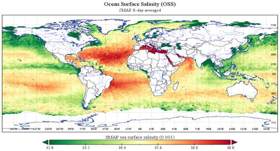
Figure 8.
Ocean surface salinity map derived from 8-day averaged SMAP observations.
Many studies have been so far conducted to retrieve OSS from the SMOS, Aquarius, and SMAP radiometers. For example, Sun et al. (2019) compared OSS data from these microwave radiometers with in situ measurements and analyzed the causes of differences. It was observed that OSS values, obtained from these radiometers were relatively less accurate in near-polar regions due to decreased temperature and a less dense network of in situ instruments in high latitudes. Moreover, Olmedo et al. (2017) compared OSS estimations from SMAP with SMOS and Aquarius in the Red Sea, which is an extreme case for OSS measurement due to the significant land contamination. It was observed that SMAP captured OSS in open ocean water with similar efficiency as the other two instruments. ML algorithms have also been employed along with microwave radiometer data for OSS estimation. For instance, Menezes (2020) estimated SMAP OSS in the Persian Gulf region using ANN, SVM, RF, and Gradient Boosting Method (GBM) algorithms. Feature importance analysis revealed the high importance of latitude in both RF and GBM algorithms [165].
2.4.3. Summary and Future Direction
Considering the effect of OSS on marine ecosystems and ocean-related economies, the future direction of OSS observation using the RS systems can contribute to ocean sustainability and monitoring studies. It is also important to investigate different RS systems for OSS estimation and select the optimal RS systems and corresponding techniques for reliable monitoring of OSS. Frequent RS measurements with reasonable spatial resolutions should be combined with state-of-the-art ML algorithms to provide accurate long-term monitoring of OSS.
2.5. Ocean Color (OC)
OC is of substantial importance in monitoring aquatic environments and in studying the biology, chemistry, and physics of oceans. The main reason for measuring OC is to study phytoplankton. Phytoplankton has a foundational role in forming the oceanic food web and is the initiation element of the food chain for most of the Earth. OC can also represent the health and chemistry of the ocean. Finally, OC information can help the fishing industry by finding suitable fishing spots that are rich in phytoplankton.
The wide variety of RS systems (e.g., satellites with different spectral, spatial, and temporal resolutions) has facilitated OC studies by developing various algorithms to derive biogeochemical and optical parameters related to OC. This has also helped to efficiently characterize the ocean biosphere properties at high spatiotemporal scales [182,183]. OC measurement using RS methods is highly required for various oceanographic applications, especially on a global scale. Due to the need for efficient environmental monitoring of the offshore and onshore oceans, there have been considerable developments in spaceborne OC technology and the corresponding algorithms in recent years.
OC can be mainly studied by analyzing the reflectance data and, thus, optical RS systems are the main instruments that have been used for OC mapping. However, it should be noted that TIR radiometers, MIR radiometers, and SAR systems have also been rarely used for OC estimation. OC mapping using optical satellites is only discussed in this section.
2.5.1. Optical
Remotely sensed OC measurements provide information about the spectrum of water reflectance and enable us to retrieve marine Inherent Optical Properties (IOPs). IOPs are the spectral absorption and scattering attributes associated with ocean water and its constituents [183]. OC is generally referred to as the spectrum of reflectance (called Rrs), which is computed as the ratio of water-leaving radiance to downwelling irradiance above the ocean surface [184]. The total radiance (Lt) from the TOA is also measured by optical RS systems.
Considering the several radiances involved in the satellite OC measurements, there are generally two main approaches in the literature that define the relationship between the intended radiance and geophysical properties [185]. The first and most common approach is based on the fact that OC applications seek to measure the spectral distribution of water-leaving radiance (Lw). Lw illustrates photons emanating from absorption and scattering processes beneath the sea surface and emit into space [183,186]. For example, a simple equation of different reflectance pertaining to satellite OC applications can be formulated as Equation (7) [187].
where the superscript TOA demonstrates radiances reaching the TOA. The atmospheric contribution () is known as the scattering caused by atmospheric gases and aerosols and multiple scattering interactions between them. The term total surface reflectance () includes the reflection of sun glint and background sky radiance from the sea surface and the contribution of their radiance, which is reflected by surface whitecaps and foam [187]. All these correction terms must ultimately be subtracted from Lt to calculate [188]. can be then converted into Rrs after division by downwelling irradiance. Finally, the geophysical properties can be estimated by applying different algorithms to Rrs.
Regarding the second approach, can be directly related to IOPs or representatives of biogeochemical properties without the obligation of implementing complicated atmospheric corrections [183,189]. Although atmospheric corrections are highly prone to be confounded by absorbing aerosols and optically complex waters, there are multiple non-conventional approaches that circumvent this prerequisite. For example, a combination of atmospheric and oceanographic methods can solve both atmospheric and marine variables at the same time. Generally, this method combines two models in which one model accounts for aerosol properties and the other one expresses water components via IOPs. Operation of the coupled atmosphere–ocean approaches is similar to semi-analytical inversion approaches. However, in these methods, the number of unknown variables in the coupled models is higher because both aerosol and marine expressions are involved. Additionally, coupled models normally need more spectral bands than conventional semi-analytical inversion approaches. By employing the existing RS OC data, coupled models use 𝐿𝑡 from the visible and NIR bands by which the retrieval of aerosol and hydrosol variables converts to a classic inverse problem. The principal privilege of coupled atmosphere-ocean approaches is that they can better account for absorbing aerosols and intense NIR radiances. Nevertheless, the coupled models have inherent limitations due to their dependence on the general formulation of the aerosol and marine components, which has been historically challenging [183].
Total marine IOPs can be considered as the sum of the contributions of common component IOPs from different water constituents, namely phytoplankton, Total Suspended Matter (TSM), and CDOM. Investigations into TSM and CDOM concentrations from RS OC data and retrieval of main IOPs of OCh, which expresses phytoplankton abundance and physiology, have been widely performed using different arithmetic algorithms. In fact, IOP retrieval of each constituent type employs different absorption and backscattering ranges and ratios of specific bands (e.g., reflectance classification algorithms, spectral band-ratios, and spectral band-difference algorithms). More approaches in this category, such as OC Chl algorithms, are widely discussed in [190,191].
The IOP retrieval algorithms of ocean water can be generally divided into two groups of band arithmetic and spectral inversion algorithms. Researchers have so far made many efforts to develop RS models to define the relationship between Rrs and IOPs. Considering Rrs as a function of IOPs (called forward model, F), after the development of an appropriate forward model, retrieving the IOPs from Rrs is possible by solving a mathematical inverse problem of F − 1. To this end, although scalar RT simulations and approximation to the RT [183] are the two main approaches; however, other approaches, such as empirical-statistical regressions and ANNs have also been utilized [192]. Several RT computations, which depend on user input IOP measurements or models as well as approximations with empirical coefficients, have been proposed to obtain Rrs [193]. Semi-analytical inversion algorithms are also a combination of empiricism and RT theory. The Quasi-Single Scattering Approximations (QSSA) as an approximation to the RT, ignores multiple scattering impact as opposed to hydrological RT algorithms and are less accurate than RT codes. The reflectance beneath the sea surface, which can be obtained from Rrs, can be approximated as a function of total absorption and backscattering coefficients in many QSSA models used in various OC applications [183,194]. In this regard, partitioning the total spectral absorption and backscattering coefficients into water constituents’ normalized absorption and backscattering coefficients, including shape and magnitude coefficients has been an imperative stage for further processes of IOP retrievals using semi-analytical inversion approaches, look-up-table approaches, empirical methods, and ML algorithms [190].
Over the past decades, many researchers have utilized various optical RS datasets to study OC. For example, temporal dynamics of coastal water turbidity have been mapped by Choi et al. [195] using the Geostationary Ocean Color Imager (GOCI) OC data. The main objective was to investigate the sedimentary processes and environments that were mostly influenced by semidiurnal tides in specific coastal areas. They developed an empirical TSM algorithm using in situ measurements of TSM concentrations and water-leaving reflectance of coastal water surface. This helped them map the temporal transformations of TSM concentrations from GOCI images acquired at hourly intervals. The assessment process was consequently performed by comparing the results with in- situ measurements and TSM concentration results yielded from the MODIS sensor. Furthermore,
Choi et al. (2014) investigated the dynamics of Dissolved Organic Carbon (DOC) as the major representative of the total organic carbon in the oceans’ coastal water and CDOM. Since DOC and CDOM are significantly important in climatic and biogeochemical cycles and have considerable effects on the estuarine ecosystem, they developed new algorithms for DOC and CDOM retrievals. These algorithms were found suitable to be applied to different regions using various RS datasets and over different water conditions [196].
There have always been several challenges of OC mapping using optical RS imagery. In this regard, it is essential to consider the necessity for documentation of IOPs’ output uncertainties and investigate the instabilities of satellite instruments in the prelaunch or on-orbit characterization. IOPs outputs are mostly affected by uncertainties of Rrs caused by sensor noises, deficiencies in atmospheric corrections, types of parameterization and approximations, as well as assumptions in the forward and the inverse solutions methods [183]. In the case of spectral inversion algorithms, the main weakness is related to finding the proper parameters of the IOP spectral shapes [193]. As discussed in Blondeau-Patissier et al. [191], the limitations and challenges of diverse algorithms differ from one another and they highly depend on the intended OC applications. Additionally, there is no universally accepted approach for IOP retrievals in all ocean waters, such as coastal water, turbid water, and complex water. Thus, they usually suffer from region-specific parameterizations. Another issue is that alterations in SST and OSS can result in volatility of thermodynamic properties and changes in marine IOPs in some spectral ranges [183].
RS techniques for OC mapping have several limitations that are mainly related to data availability, sources of uncertainties in remotely sensed biomass and diffuse attenuation, sub-surface estimations, as well as seasonal and regional variations in phytoplankton photosynthetic parameters. These issues are more challenging in Arctic oceans due to frequent SI and cloud presence. Additionally, the near-surface fogs and clouds, which are typically caused by the melted SI in Polar regions, increase in summer. Therefore, the challenges increase in summer times mainly due to a lack of suitable RS observations [150].
ML algorithms have been reported to resolve some of the challenges discussed above. It was also reported that a combination of physical and DL models is a promising approach to reducing the limitations of the traditional RS models for OC mapping [197]. For example, Nock et al. (2019) [198] developed a CNN architecture to parameterize the water column, including depth, bottom type, and IOPs, using 89 spectral bands of hyperspectral images. Moreover, combining the spatiotemporal autocorrelation and heterogeneity of oceanographic variables within a DL model or designing the spatiotemporally constrained DL models could be a practical solution for many challenges in future OC studies. Finally, it should be noted that despite the numerous advantages of DL techniques, their use for OC retrieval is limited due to the need for large in situ samples [197].
2.5.2. Summary and Future Direction
The future of OC using RS methods heavily relies on our ability to plan beyond a single sensor mission and to provide long-term, high-quality, traceable satellite reflectance measurements. These capabilities along with coupling between missions as well as calibration and validation exercises could result in having more reliable multi-decadal datasets. Along with the parameters derived from OC, many satellite-derived variables, including photosynthetic-active radiations, OSW, rainfall, and OSS could be combined to provide better opportunities for studying OC.
2.6. Ocean Chlorophyll (OCh)
Phytoplankton is the main photosynthesizer in oceans providing the ocean’s food chain and primary production [182,199]. Therefore, investigating the impact of principal phytoplankton groups on marine ecosystems and global biogeochemical cycles has long been a hot research topic. In this regard, Chl concentration as a biological property along with phytoplankton absorption coefficient as an optical property can be considered as the key information about phytoplankton biomasses. Since Chlorophyll a (Chl-a) is the main pigment involved in photosynthesis, it has been mainly studied to monitor and analyze phytoplankton concentrations in many ocean studies. Ocean Chl-a studies help to understand the reaction of the marine ecosystem to human activities and facilitate detecting and monitoring eutrophication [199]. Moreover, estimating Chl-a concentration at the ocean surface can help in identifying potential fishing zones [200]. Finally, observing the spatiotemporal distribution of Chl-a concentration can reveal the ocean’s role in climate change [182].
The global distribution of Chl-a has been reported to be rich in areas located along the coasts and continental shelves, especially in the north of the northern hemisphere [191]. Temperate Chl-a concentrations have also been observed in the south of the 45th parallel south [191]. Although coastal waters account for a small portion of the Earth’s ocean water, they contain almost a quarter of the global marine primary production and represent the effect of coastal detrimental phytoplankton blooms on human activities [199]. Therefore, coastal waters have been the major focus of most studies investigating the variability and concentration of Chl-a [185,199].
Although various RS systems, such as optical, TIR radiometer [201], microwave radiometer [202,203], and SAR [204,205] have been used for Chl-a mapping, optical OC systems have been most frequently used for this application. Therefore, Chl-a mapping using only optical RS systems is discussed in this section.
2.6.1. Optical
Chl-a can be studied using optical RS imagery due to its effects on ocean water. For example, the color of ocean waters can be affected by phytoplankton blooms. Phytoplankton blooms either raise light backscattering due to the spectrally localized water-leaving radiance minima of Chl-a or increase especial algal pigments absorption in some of the algal species [191]. Furthermore, similar to the process of IOP retrievals of ocean water constituents from RS measurements, the absorption and backscattering properties of Chl-a as the spectral marine IOPs can be estimated by applying bio-optical algorithms to Rrs.
Generally, water reflects electromagnetic energy in the visible up to the NIR ranges of the spectrum. As shown in Figure 9, all energy beyond 1.2 μm is absorbed by water. The spectral signatures of three types of water, including ocean water, turbid water, and water with chlorophyll are provided in Figure 9a. Chl-a mainly reflects green and absorbs most energy from wavelengths of violet-blue and orange-red light whose reflectance makes chlorophyll appear green. Figure 9b illustrates the absorption spectrum of both Chl-a and Chl-b pigments. This pigment characteristic offers a basis for Chl-a estimation from blue-to-green ratios of RS reflectance in clear oceanic waters.
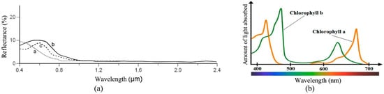
Figure 9.
(a) Typical effects of chlorophyll and sediments on water reflectance [205]: graph a, b, and c indicate ocean water, turbid water, and water with chlorophyll respectively; (b) the absorption spectrum of both the Chl-a and the Chl-b pigments [185].
The approaches applied by the RS community to estimate Chl-a from Rrs can be categorized into the following groups: empirical, semi-analytical [184], and ML models.
Empirical algorithms statistically relate in situ measurements of Chl-a and Rrs (radiance or reflectance in narrow bands) observed by an optical system [182,190,191,200]. The reflectance band-ratio and spectral band difference algorithms are the most common empirical methods for Chl-a estimation. The blue-green (440–550 nm) spectral band ratio, Tassan’s approach [206], linear red-edge ratio methods [207], and OC band-ratio algorithms (e.g., OC2 [208] to OC6 [190]) for SeaWiFS and their corresponding versions for other OC sensors are the examples of the reflectance band-ratio algorithms. Among these methods, the empirical blue-green spectral band ratios have been widely utilized. Blue-green ratios are mainly applicable for open ocean waters because they show less sensitivity to changes in Chl-a concentrations in optically complex coastal waters [191]. Regarding the spectral band difference algorithms, diverse band triplets from the red-NIR or the blue-green spectral ranges can be used. The fluorescence line height algorithm [209], maximum Chl index [210], which can be only applied to MEdium Resolution Imaging Spectrometer (MERIS), color index algorithm [211], which is applicable to SeaWiFS, MODIS, and MERIS, are the popular spectral band difference algorithms.
Semi-analytical algorithms are developed by a composition of empiricism and simplified RT models [190]. Semi-analytic bio-optical models have allowed us to simultaneously estimate Chl, suspended particulate matter, and absorption by CDOM, which can potentially be more efficient for optically complex waters (e.g., coastal waters) [212]. For this purpose, spectral shape functions have usually been assumed for all constituent absorption and scattering components of ocean water. Additionally, linear or nonlinear inversion methods have been employed to retrieve the magnitudes of constituents, which are required for matching the spectral distribution of Rrs [190].
Multiple ML-based algorithms, such as ANN and SVM, have also been applied to Chl-a concentration estimation [213,214]. The non-linear and complex nature of the measurements provided by OC sensors and the need for techniques declining high-dimensional data have recently encouraged the RS community to produce high-dimensional predictors using different models of DL [215]. Due to the complexity of the marine environment, many DL algorithms have been used to ameliorate the precision and reliability of empirical-predictive methods [216]. ML algorithms can tackle the difficulties associated with traditional empirical modelling for Chl-a retrievals, hence modelling non-linear relations between dependent (Chl-a) and independent variables [216]. The popular approach to training ML models is often supervised learning using match-ups from in situ Chl-a measurements and Rrs data (known input-output pairs) [216,217]. Many studies (e.g., [214,215,216,217,218]) have so far demonstrated the superiority of various ML methods in comparison with conventional approaches for Chl-a concentration estimation using RS data.
There are numerous RS studies focused on ocean Chl-a retrievals. For instance, Loisel et al. [219] delineated the spatiotemporal patterns of the Chl-a concentration in the Vietnamese inshore waters using OC RS data which was acquired by MERIS between 2002 and 2012. To this end, a wide range of in situ data of Chl-a, Rrs, and IOPs was collected from different parts of the Vietnamese coastal waters. Subsequently, they evaluated different Chl-a inversion algorithms utilizing the aforementioned in situ data. The functionality of the most appropriate bio-optical algorithm was also investigated considering the geographical location and bio-optical environment. After applying the best algorithm to the monthly RS reflectance data of MERIS, they also analyzed the temporal variability trends of Chl-a. Moreover, a comprehensive study to develop the Chl-a algorithms for 25 OC RS systems has been conducted by Blondeau-Patissier et al. [190] using 65 different empirical algorithms. They aimed to fulfill consistency and comparability among Chl-a algorithms which is required for synthesizing data from overlapping OC missions of various sensors. This process led to a considerable increase in coverage of accessible data over the global ocean and resulted in expanding the existing time series. They also introduced their expanded versions of the OC algorithms in which the 412 nm band was utilized in the maximum band ratio.
Despite the advantages of optical RS systems in estimating Chl-a concentrations, there are still several challenges restricting the application of Chl-a algorithms. For example, A single OC sensor cannot be solely utilized to evaluate long-term Chl-a changes due to its limited operation time. Moreover, combining Chl-a data from multiple sensors augments their global coverage especially in cloudy regions of cloudy seasons. However, this data combination faces several challenges. Inadequate quality of Chl-a multi-source data calibrations can degrade the overall quality of Chl-a estimations. Overall, inconsistent and incomparable atmospheric correction algorithms, and inconsistency of the geophysical algorithms utilized for different sensors can negatively affect the accuracy of multi-instrument Chl-a products [191].
Moreover, considering the dependence of passive OC sensors on daylight measurement of reflectance, multiple regional, seasonal, and latitudinal differences could occur in Chl-a mapping. This can also affect long-term studies of Chl-a. Consequently, most long-term approaches suffer from latitudinal and seasonal biases and contain errors due to coverage gaps [190]. Additionally, estimating Chl-a concentrations in optically complex waters is highly required because the optical properties of these water regions may differ from multiple assumptions in the algorithms. This difference may result in creating large errors in the produced Chl-a maps [212]. Finally, multiple studies (e.g., [191,220]) have reported that optical RS systems cannot always sense deep Chl maxima. Consequently, ocean Chl-a observations are restricted to specific optical depths [221].
2.6.2. Summary and Future Direction
The coastal ocean accounts for almost one-third of all marine biological productivity in the world. Most studies have shown that retrieval of Chl-a concentrations in complex coastal waters is more challenging than in open ocean waters, especially when band-ratio algorithms use blue and green bands. This is because the impact of CDOM and TSM at those wavelengths adversely affects Chl-a retrievals [191]. Since the spectral range of the red and NIR bands is less affected by these two optically active constituents, the great potential of band ratios using the red and NIR bands for Chl-a detection in coastal waters deserves much more attention in future studies.
Over recent years, significant advances have been made in the development of bio-optical models in coastal waters focusing on the use of specific IOPs for detecting phytoplankton blooms instead of the historically used Chl-a proxy. Evaluating the accuracy of bio-optical algorithms for detecting phytoplankton blooms in coastal waters is required in the future. While there are currently few optical and biogeochemical in situ datasets which characterize pre- and post-blooms conditions, automated sensors, such as autonomous underwater vehicles equipped with bio-optical sensors, can be helpful in the future.
It is also expected that hyperspectral sensors with higher spectral and temporal resolutions could improve the development of efficient OC algorithms and, thus the algorithms of Chl-a retrievals.
2.7. Ocean Oil Spill (OOS)
The importance of petroleum for human life and industry is undeniable. Every day, numerous ships move oil and, consequently, this high amount of travel increases the risk of OOS pollution. Generally, OOS may occur due to two primary reasons [222]. The first reason is transportation accidents. For instance, a Tunisian cargo ship had a collision with an anchored Cypriot container ship in the Mediterranean on 7 October 2018 [223]. Although no one was injured in this accident, it caused a fuel leak of about 600 tones. The second and the most prominent reason is the oil waste illegally discharged by tankers [222,224]. The tankers consider illegal waste discharging the most economical option because the chance of being caught is slight and the risk of fines is low [222,225].
When the oil is spilled on the ocean surface, it tends to form a thin layer, called an oil spill or oil slick. Ocean wind and ocean currents spread the OOS over a wide area [226]. OOS can cause severe issues to the marine environment. It can also negatively impact the population of sea birds and fish. Moreover, phytoplankton and aquatic organisms that play an essential role in the food chain are severely affected by OOS. Finally, people with livelihoods based on fishing and tourism intensely suffer from this pollution [226,227,228].
Among various approaches for OOS study, RS is the most cost-effective technology. It helps to collect valuable information about the spills, such as the size and extent, which are critical for cleaning up the pollution before they cause widespread damage [222]. It is suggested that the combination of satellite and airborne RS datasets must be applied to create an effective OOS surveillance system [222]. In such a system, satellite data are first used to search a wide area and rapidly identify OOS candidates before they spread over the ocean. Then, aircraft images are applied for a detailed analysis and the collection of legal evidence to identify the possible polluter [222].
There are different types of RS systems that can be effectively used for OOS detection. Table 5 summarizes these systems and their advantages and disadvantages for OOS studies.
Table 5.
Different RS systems for OOS detection along with their advantages and disadvantages.
Among these, SAR and optical RS systems have been widely used for OOS mapping and monitoring. Although optical sensors have been used for OOS detection [229,230,231], they only acquire images during the daytime. Furthermore, they cannot provide useful images in cloudy days/regions and inclement weather conditions [226,232]. However, airborne optical systems (e.g., hyperspectral sensors), which do not have these limitations, have frequently been employed for OOS mapping. However, the high dimensionality of hyperspectral images causes challenges in the transmission, storage, and processing phases. Additionally, a well-known phenomenon, called the curse of dimensionality, decreases the accuracy of the classification of these datasets. More importantly, hyperspectral sensors are expensive and mostly publicly unavailable compared with multispectral and microwave RS systems [233]. Several studies on OOS successfully applied hyperspectral systems. For example, Lu et al. (2013) [234] applied a normalization method to retrieve the oil slick thickness within a specific range using Hyperion data. Moreover, Wang et al. (2021) [235] developed a CNN model to employ both spectral and spatial information of hyperspectral images for classifying OOS into thick and thin oil classes. Moreover, Zhu et al. (2019) [236] combined spatial information and the Stacked Autoencoders neural network for OOS classification using Airborne Visible/Infrared Imaging Spectrometer (AVIRIS) data.
In summary, SAR systems provide data both day and night without being affected by bad weather conditions. Thus, SAR systems attract more attention to OOS studies [224,226]. In the following subsection, more details of OOS mapping using SAR data are provided.
2.7.1. SAR
OOS makes the oil-covered surface smoother than its surroundings by diminishing the Bragg waves of the ocean surface. Consequently, as illustrated in Figure 10, the oil-covered areas appear as dark spots in a bright background of seawater in SAR images [222]. In fact, the contrast between OOS and its surrounding is a crucial factor for the successful detection of OOS using SAR data. The contrast depends on wind speed, the type and amount of pollution, OWH, and two important sensor parameters of polarization and wavelength [222].
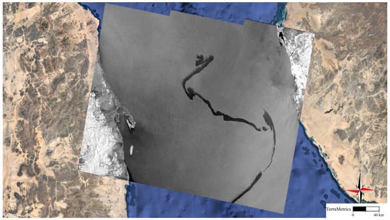
Figure 10.
An OOS caused by the explosion of Sabity Oil tanker in the Red Sea. The spill looks darker than its surrounding because it has lower backscattering values. The image was acquired by Sentinel-1 on 11 October 2019.
Although OOS is detectable in wind speed values between 2 and 12 m/s, the ideal range is 5–6 m/s [237]. Ocean surface relatively appears smoother for areas with low wind speed in SAR images. In this condition, there will be no backscattering from the ocean surface. This makes OOS detection impossible because there will be no contrast between the spill and its clutter (i.e., water) [222]. On the other hand, spills, especially thin ones, are invisible in high wind speed conditions. This is because the spills are sunk into the water for regions with high wind speed values [224,238,239].
SAR images with X (2.4–3.75 cm) and C (3.75–7.5 cm) bands are the most appropriate datasets for OOS detection. This is because they have the same scale as the Bragg waves. Additionally, the spills are more detectable in VV polarization because it has a larger backscatter from the ocean surface than the other polarizations [222,227,240]. Several research works have studied the feasibility of dual-pol and quad-pol SAR images for OOS detection. Although it is argued that SAR polarimetry improves the accuracy of the discrimination [224], processing polarimetric images is computationally expensive and costly. Quad-pol features, including a polarimetric entropy, anisotropy and span [241], mean scattering angle [224], and conformity coefficient [242], were more utilized for OOS detection. Regarding dual-pol images, the standard deviation of co-polarized phase difference [243,244,245], co-polarized correlation coefficient [246], and the degree of polarization [247] have been widely applied to detect OOS.
The major drawback of SAR images for OOS detection is the presence of other dark structures called lookalikes. The lookalikes are phenomena with similar behavior as OOS. These phenomena are usually caused by various factors, such as low wind speed, wind-sheltered by land, rain cells, zones of upwelling, ocean or atmospheric fronts, and grease ice [244,248]. Therefore, the most critical challenge of employing SAR data for OOS detection is accurately discriminating the OOS from OOS lookalikes. It is worth noting that there is also a similar challenge for optical sensors. For instance, sun glints and wind sheen may cause lookalikes in the optical sensor [226].
OOS mapping using SAR images generally contains three steps: (1) segmentation; (2) feature extraction; and (3) classification. More details of each step are provided below. In the first step, the dark regions which contain the OOS and lookalikes are extracted from images after a series of preprocessing steps, including land masking, radiometric and geometric corrections, speckle reduction, and incidence angle correction. The thresholding methods are generally applied to separate the dark area from the SAR images. Adaptive thresholding was utilized in several studies [239,249] and found to be a better option than global thresholding methods, such as the Otsu algorithm. For instance, several studies employed a segmentation method based on the Laplace and difference of Gaussian [250,251]. The feasibility of the wavelet transforms and a hidden Markov chain model was also studied in [252,253]. Additionally, a well-known constant false alarm rate algorithm was applied to identify dark regions [254]. The clustering algorithms have the feasibility in the detection of dark regions. For example, Barni et al. (1995) [255] applied a fuzzy c-mean algorithm. A combination of opening and closing as two mathematical operations was also adopted by Gasull et al. [256] to detect suspicious spills.
In the feature extraction step, several discriminative features are extracted from the dark regions obtained from the first step. Feature extraction is the most crucial and challenging step in OOS detection. A series of features describing OOS and lookalikes are extracted in this step. The extracted features must be adequately discriminative to facilitate the following classification step (i.e., the third step). The proposed features can be summarized into four main groups [224].
- Geometrical features: OOS generally has a regular shape. For instance, sailing tankers that illegally discharge oil waste form a linear spill. The geometrical features provide useful information about the shape of the identified dark regions. The following geometrical features are the most well-known features for OOS detection using RS data:
Spill area (A), Spill perimeter (P), Spill width, Spill complexity (), and Hu moments [257,258].
- Radiometric features: radiometric features provide information about the physical property of the segmented areas and their surrounding based on the backscattering coefficient (σ0). The well-known radiometric features are the average and standard deviation of σ0 inside and outside dark regions [239,258], maximum and mean contrast between dark area and background [258], maximum, mean, and standard deviation gradient of dark region’s border [258], local area contrast ratio [239], power-to- mean ratio of background [239], and the homogeneity of background [239,259].
- Texture features: these features provide information about the spatial correlation between neighboring pixels [224]. The most commonly used texture features are those obtained from the GLCM (e.g., contrast, dissimilarity, homogeneity, angular second moment, and energy and correlation) [259], statistical features after applying a discrete wavelet transformation (e.g., the logarithm of energy, Shannon’s index, angular second moment, and entropy) [260], and fractal [261,262].
- Ancillary information: in addition to the above-mentioned features, several features were proposed to facilitate discriminating between OOS and lookalikes. These features are wind speed, the number of ships in the image [238], distance to ships and lands [263], and weather information [264].
In the final step, a classification algorithm is trained based on the extracted features to discriminant the OOS from lookalikes. Various classifiers have been applied in the literature, including ANNs [258], Mahalanobis classifier [257], SVM, fuzzy classifier, an algorithm based on a statistical model and rule-based approach [239].
2.7.2. Summary and Future Direction
OOS detection using RS technology has several limitations: (1) there is a lack of open-source annotated datasets that have been compiled from numerous multisensory sources in various places; (2) to discover optimal parameter configurations, fine-tuning of hyperparameters of ML models necessitates substantial trial-and-error testing; (3) the literature lacks a detailed classification of oil spills/slicks, including oil type, thickness, and other chemical parameters; (4) many RS images are accessible; however, the traditional method of image downloading, preprocessing, and core processing should be replaced by web processing algorithms. Given the ongoing advancements in RS technology, cloud computing services, computer vision methods, and the growing availability of publically annotated RS data, the aforementioned issues could be reduced in the future [265].
There is a clear requirement for server-based algorithms to process images in the cloud. A new type of in situ measurement is also required, such as tiny and low-cost buoys that measure the type of oil and its chemical composition, as well as small UAVs for high-resolution monitoring tasks. Given their strong discriminating capabilities, hyperspectral sensors will have more attention in the future, particularly when combined with UAVs for OOS detection [2]. Furthermore, future approaches will use more background auxiliary information, such as OSC, OSW, and Chl-a distribution, to increase OOS detection accuracy [255,266].
Recently, several DL algorithms have been developed for OOS detection from RS data [267,268,269,270] with very high accuracy. These algorithms merit robust feature extraction and autonomous learning capabilities, paving way for the automatic and rapid detection of OOS by clearly distinguishing OOS from lookalikes [271,272]. Thus, it is expected more DL models along a combination of various RS datasets will be applied for OOS monitoring in the future.
2.8. Underwater Ocean
RS has several applications for underwater ocean environments. In this study, three important applications of bathymetry, Aquatic Vegetation (AV), and Coral Reef (CR) using different types of RS systems are discussed.
Bathymetric data provide the depth of water bodies as a function of geographical coordinates [273]. Bathymetric mapping is important in planning near-shore activities (e.g., pipeline laying, port management, dredging operations, oil drilling, and fishing), navigation, oceanography, marine geology, and paleoclimate research [273,274,275]. Additionally, accurate bathymetry maps are required for marine power plant planning, storm surge modeling, and coastal management [2].
AVs, including all underwater flowering plants, play a critical role in aquatic ecosystems. For example, AV provides food and habitat to wildlife [274,276,277], and is important for biogeochemical cycling [278], sediment stabilization and trapping [279], nutrient uptake [280], as well as wave attenuation and hydraulic resistance [281]. Despite various ecological, physical, and economic benefits of AVs, they are disappearing mainly due to climate change and anthropogenic disturbance, especially in coastal areas [282,283]. Given the importance of studying AV, several national and international protocols and frameworks, such as hyperspectral RS protocol development for AV mapping and monitoring in shallow waters [284], have been proposed.
CR is home to at least 25% of all marine species [285]. CRs provide different ecosystem services, such as flood protection [286], tourism [287], coastline protection [288], fisheries, and food sources to millions of people [289]. For example, it was estimated that nearly 500 million people worldwide depend on CRs [290]. CR is very sensitive to changes in hydrodynamic settings (e.g., water quality, light, and temperature), and can only thrive in a restricted domain of environmental conditions [291,292]. Based on the most recent report from the global CR monitoring network in 2008, 54% of the world’s CRs are suffering from regional or global threats [293]. This is mainly related to the side effects of climate change and anthropogenic disturbance [288,293]. The increasing global awareness of the importance of CR, on the one hand, and the necessity of detailed mapping and classification of CRs based on actions 15 and 17 of the reef 2050 long-term sustainability plan [294], on the other hand, have been leading to conducting a wide range of CR programs worldwide.
Despite the importance of underwater ocean studies, there are still challenges in generating adequate data on global oceans due to the large extent and limited accessibility in the ocean environment [273]. For instance, it is estimated that 70% of the world’s littoral zone has not yet been mapped based on modern standards [279]. In recent decades, several methods have been investigated to obtain accurate information about ocean topography, AV and CR, ranging from field surveys to RS methods (see Figure 11).
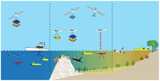
Figure 11.
Summary of approaches applied to underwater studies [295].
Field surveys are time-consuming, expensive and have accessibility issues [277,296]. On the other hand, a pre-measured cable or rope located on ships, which was historically used to collect bathymetric data, is sometimes inefficient because it can only provide point-based information [273]. The shipborne methods, such as echo sounding, are relatively efficient for underwater studies [274]. However, these methods are also limited over large remote ocean areas mainly due to the high cost [297,298]. Additionally, the applicability of this technique is negatively affected by technological restraints and environmental conditions in coastal regions [299]. Airborne and spaceborne RS methods, however, can effectively address several limitations of field surveys and shipborne methods. RS methods are safer, cost-effective, and faster than field surveys. For example, Mumby et al. [300] reported that six days of field survey is equal to 20 s of airborne acquisition time. Furthermore, the consistent archived and frequent observations of spaceborne RS systems allow for identifying underwater changes over time in a cost-efficient manner.
Both airborne and spaceborne RS systems have been of interest in underwater studies since 1975 and the interest has grown on an annual basis [301]. Table 6 summarizes the advantages and disadvantages of the most important RS systems for underwater studies. The application and details of each of these systems are also discussed in the two following subsections of bathymetric and AV/CR mapping.
Table 6.
Different RS systems for underwater ocean studies along with their advantages and disadvantages.
2.8.1. Bathymetric Mapping
Optical, SAR, altimeter, LiDAR, and SONAR systems have been widely used for bathymetric mapping. To date, several algorithms have been developed to extract bathymetry information from the corresponding datasets. The analytical [302], semi-analytical [303,304], approximation [305], and optimization of analytical and semi-analytical [306] models are some examples in these regards. Although the analytical and semi-analytical algorithms can simultaneously generate various bathymetric information (i.e., water optical properties, benthic albedo, cover, and depth), they are complex [307]. On the other hand, the approximation equations can contain multiple residual errors and they require pre-processed RS data [305]. Additionally, when multi-temporal approaches are implemented, consistent water reflectance is required in these models [308].
Optical
Optical multi-spectral satellite-derived bathymetry is based on the statistical relationships between the in situ measurement of water depth and image pixel values. The blue spectrum (0.45–0.52 µm) can be used for optically sensing bathymetry because of its high penetration capabilities [297,298] (see Figure 12).
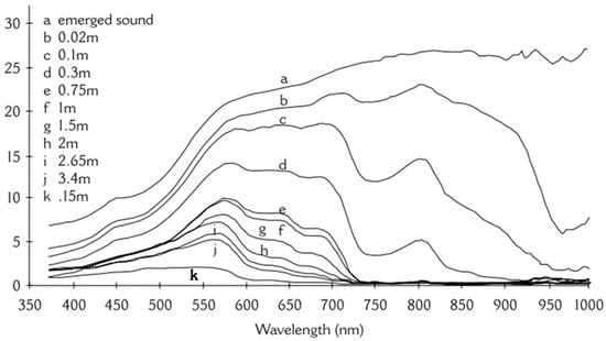
Figure 12.
Reflectance spectra of water at different depths [309].
During the past decades, a vast number of algorithms varying from empirical (e.g., band rations, logarithmic-transformed models, and ML models) to physics-based models have been developed for bathymetric mapping using optical satellite imagery [302,304,310].
Optical RS imagery usually has a lower cost, high spatial and temporal resolutions, and wide coverage, making them appropriate for underwater ocean and bathymetric studies [311]. The most important limitation of optical techniques in bathymetry is the certain, fairly restrictive conditions in which spectrally based bathymetric mapping is feasible [312]. The results of optical bathymetry are primarily reliable in clear and relatively shallow waters. Since most of the earlier studies attempted to estimate the underwater topography in shallow streams conducive, this limitation of optical-based bathymetry remains undiscovered [313]. On the other hand, to estimate the relationships between topography and pixel values, these techniques have a large amount of in situ data, which makes them inappropriate for many studies. Shen et al. (2019) [314] assessed the capability of GF-2 for shallow water bathymetry mapping by applying three different techniques of single- band regression, dual-band ratio, and multi-band regression. Based on the results, the dual-band ratio and single-band ratio methods showed the highest and lowest accuracies, respectively. Additionally, it was observed that GF-2 was a suitable alternative for the expensive Worldview-2 images for bathymetric mapping.
SAR
SAR is an active solution for measuring underwater topography down to the depth of about 100 m using emitting and receiving a microwave pulse, the frequency of which ranges from hundreds of MHz to tens of GHz [315]. Although microwave pulses cannot penetrate water, SAR can indirectly estimate the ocean bottom topography using the variations in the small-scale sea surface roughness [316]. The underlying concept is that the bathymetric features are distinguishable from SAR data of the water surface when currents are flowing over them. Regarding SAR data, [317,318,319,320] developed the first theories describing the radar imaging of underwater bottom topography. However, these theoretical models are not capable of estimating underwater bottom topography from SAR data alone. In other words, there is a need for other accurate measurements (e.g., SONAR or optical data) to be combined with SAR data and to estimate seafloor topography. In this regard, Pleskachevsky et al. (2011) [321] synergistically applied the optical data from QuickBird satellite and TerraSAR-X data to retrieve the bathymetric information. Using this fusion, they obtained water depths between 20–60 m.
Moreover, Pereira et al. (2019) [322] explored the Sentinel-1 C-band SAR images for bathymetric estimation of the Aveiro (northwestern Portugal) study site. To investigate the proposed approach in retrieving the nearshore bathymetry, they considered four high temporal resolution images. Additionally, they analyzed the sensitivity of the results to both offshore and local internal factors related to the estimation of the wavelength. Their results showed that a combined solution that merges the results of all the images slightly improved the results.
Altimeter
OWH measured by altimeter is affected by various static or dynamic characteristics, such as gravity, tides, ocean currents, El Niño, and the dynamics of basin circulation. Since the mountains on the seafloor add extra pull to Earth’s gravity field and draw more water around them, the effect of ocean bottom topography on OWH is 100 times greater than other oceanographic signals [323]. Moreover, a bathymetric signal is expressed in a shorter-spatial scale than the other oceanographic signals and, therefore, is readily distinguished [324]. These facts make altimeters promising tools for globally uniform reconnaissance of deep-sea bottom topography. Estimating the shape and structure of the ocean bottom using altimeters is called altimetric bathymetry [325].
To investigate the performance of altimetric bathymetry in retrieving topographic profiles, Salameh et al. (2018) [326] compared the bathymetry from four altimetry missions (European Remote Sensing 2 (ERS-2), ENVISAT, Satellite with ARgos and ALtiKa (SARAL), and CryoSat-2) with the LiDAR-derived topography over the intertidal area of the Arcachon Bay. They found that SARAL and CryoSat-2 with a Root Mean Square Error (RMSE) of lower than 0.44 m provided more accurate bathymetric maps than LiDAR.
Altimetric bathymetry has many scientific and commercial applications, such as numerical ocean modeling, fisheries, and locating obstructions/constrictions to the major ocean currents. However, they do not have sufficient accuracy and resolution for assessing navigational hazards [327].
LiDAR
LiDAR is another active RS system that estimates the physical characteristics of the seafloor mainly using a green laser pulse (532 nm), with a laser repetition frequency of approximately 10 KHz [328,329]. LiDAR emits a light pulse that can penetrate through the water column and then receives the returning signal to measure the range of the seabed [330]. As such, the returning signal from the ocean can be analyzed to provide high-resolution ocean floor topography. LiDAR systems have proven to be remarkably useful in mapping seamless, coastal topographic–bathymetric due to the high penetration in ocean water (nearly three times deeper than passive RS systems) [329,331].
Both airborne and spaceborne LiDAR systems have been employed for bathymetric mapping. Regarding accuracy and speed, airborne LiDAR systems are very promising for obtaining underwater topography in coastal areas [332]. They can measure the ocean floor topography with a spatial resolution smaller than 1 m and vertical resolutions of around 15 cm [333]. However, they are not relatively cost-efficient, reducing their applications, especially over areas where airplanes have difficulties getting close to them [334,335]. Although spaceborne LiDAR systems have been developed since 2003, their applications were limited until 2018 when the Ice, Cloud, and Land Elevation Satellite-2 (ICESat-2)), which carries the photon- counting LiDAR sensor (i.e., Advanced Topographic Laser Altimeter System (ATLAS)) was launched [336]. This spaceborne LiDAR system has been employed to determine ocean floor topography, as well as the mass balance of the polar ice sheets and their contributions to global sea-level change [337]. For example, Ma et al. (2020) produced the bathymetric maps based on empirical linear and the band ratio models using ICESat-2 and Sentinel-2 imagery. Ma et al. (2020) also employed the bathymetric points derived from ICESat-2 instead of the in situ auxiliary bathymetric points to train the traditional empirical linear and band ratio models. Then, bathymetric maps for an area in the South China Sea were produced using the trained empirical models and Sentinel-2 multispectral images. These studies provided evidence that ICESat-2 has the potential to reach a sub-meter bathymetric accuracy (nearly 10% of the maximum depth of water) in shallow and clean water areas after calibrating the bathymetric errors [336]. However, compared to the other RS bathymetric techniques, spaceborne LiDAR systems have multiple disadvantages. For example, they are subject to bathymetric inaccuracies in turbid water [329]. Moreover, some other error resources, including the SL variability persuaded by tides and waves, the non-nadir incidence, the refraction effect of sloping sea surface and water column, and inherent water properties reduce the accuracy of these systems [338,339].
SONAR
SONAR, in general, is a shipborne RS technique that has revolutionized oceanography and bathymetry. Based on the technique of receiving and recording pulses, SONAR instruments can be categorized into single-beam SONAR, multi-beam SONAR, synthetic aperture SONAR, and side scan SONAR [340]. The most frequently used SONAR systems for seafloor mapping are multi-beam SONAR and side-scan SONAR. Multi-beam instruments, also known as MultiBeam EchoSounders (MBES), mounted on the ship’s hull determine the seafloor topography by transmitting sound signals and receiving the echo from the seafloor to measure the round-trip time taken during the transmission period [341]. Unlike multi-beam SONAR, which measures the timing of echoes, side scan SONAR measures the strength of echoes. Therefore, side-scan SONAR produces black-and-white photographs of the seafloor, instead of topography data [342]. As such, Multi-beam SONAR is usually used for bathymetric mapping of the seafloor for mapping both shallow and deep waters and also updating nautical charts [331].
It should be noted that there is another classification of SONAR systems: active and passive. Although both of these instruments employ sound echoes for bathymetric mapping active SONAR is emitting pulses of sounds and listens for echoes. However, passive SONAR is principally listening for the sound made by other targets (e.g., whales and other vessels) [343].
The accuracy of SONAR systems is affected by boat pitch, roll, and yaw. Moreover, SONAR techniques are usually more expensive and time-consuming than airborne and spaceborne bathymetric systems, making them inappropriate for many applications [344]. Several studies have attempted to reduce these errors. For instance, Bio et al. (2020) [345] integrated depth measurements from a low-cost single beam sonar with a dual-frequency differential high-precision GNSS data for shallow water bathymetric mapping. Given this technique, they attempted to eliminate the need for applying the method based on tidal corrections, which always introduce several uncertainties. They also eliminated the influences of boat pitch, roll, and yaw on depth measurements.
Summary and Future Direction
Satellite derived bathymetry has gained popularity among scientists because of its synoptic coverage and capacity to collect information from inaccessible locations. Bathymetric mapping research is currently focusing on the efficacy of providing operational products, with the future focusing on real-time operational application in ports, harbors, channels, creeks, etc. In this manner, several satellite agencies are currently debating the current constraints of best-fit sensors for precision data collecting for bathymetric mapping, particularly in shallow waters of coastal regions.
In the case of classification tasks, the hybrid approach undeniably offers the opportunity to think beyond the horizon of conventional methods/algorithms. Some of the constraints, such as chlorophyll, turbidity, and other parameters in the complex water bodies pose significant challenges that has fallen by the wayside in bathymetric mapping literature for the past several years. To address these challenges, accurate datasets, as well as advanced statistical and machine learning models are required.
2.8.2. AV and CR Mapping
Optical, SAR, LiDAR, and SONAR datasets have been widely used for AV and CR mapping. AV and CR mapping methods using RS data can be generally divided into two groups of empirical and physical models [295]. Empirical models focus on the empirical relationship between in situ and RS data [346]. On the other hand, physical approaches utilize prior knowledge about AV and CR based on RT models [295,347], which simulate the attenuation of the irradiance through the atmosphere. RT models require a considerable amount of input parameters, the optimization of which increases the computational cost and the amount of effort. In the following subsections, the applications of different RS systems for AV and CR mapping are discussed.
Optical
The number of extracted AV and CR classes and the level of accuracy of optical RS methods directly depend on the environmental conditions (e.g., water quality, water depth, and sea surface situation) and optical sensor characteristics (spatial, spectral, and temporal). If water quality is suitable and the seabed is visible, AV and CR can be reasonably mapped. However, if the seabed is invisible, mapping is almost impossible, even after the optical imagery is enhanced [295]. Moreover, Due to the air-water interface issues, the spectral differentiation of AV and CR using optical sensors needs specialized strategies [346]. The spatial resolution is also important for accurate AV and CR mapping. For example, very high spatial resolution images acquired by UAVs are commonly used for this purpose over relatively small areas and near coastlines. Moderate and high spatial resolution optical datasets (e.g., those acquired by Landsat and SPOT) are also common for this application over relatively large areas with acceptable accuracies [346,348]. Furthermore, it has been argued that the spectral resolution of optical sensors plays an important role in the detection and classification of AV and CR types [346,349]. Therefore, selecting a suitable sensor with a proper number of spectral bands (e.g., hyperspectral sensors), which can effectively identify small spectral differences, is very important for accurate AV and CR classification (see Figure 13).
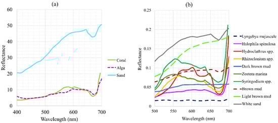
Figure 13.
Spectral signatures of different (a) CRs [349] and (b) AVs [295].
Many studies have employed optical datasets for AV and CR classification. For instance, Ghirardi et al. (2019) [350] mapped the extent of AV in Lake Iseo, Italy, between 2015 and 2017 based on in situ measurements and 22 Sentinel-2 images. For this purpose, a physical inversion model was applied to classify bare sand and AV classes. Inter- and intra-annual fluctuations in lacustrine spatial coverage, patterns of AV, and intense uprooting phenomena were also recorded in this study. The proposed method for mapping AV was concluded to be robust with acceptable accuracy. Moreover, Roelfsema et al. (2018) [351] combined an object-based image classification method and an ecological model for CR habitat mapping in the Great Barrier Reef. It was observed that the combination of Landsat-8 with geomorphic-ecological models could provide satisfactory results over a large area. Additionally, Visser et al. (2013) [352] discussed the application of optical RS for AV mapping using statistical and ML algorithms. They studied the role of spatial and textural information for improving the discrimination of AV species using very high-resolution optical images. Their results showed that water depth was a limiting factor for AV species mapping from optical RS images. It was also observed that shape and texture information could improve the accuracy of the detection of AV species.
LiDAR
LiDAR has also been applied in the marine environment to map and monitor AV and CR [353]. Not only LiDAR can sample the depth of the seabed along straight lines in clear water, but it can also estimate the intensity of returning light pulse. Therefore, various LiDAR-derived indices can be efficient proxies for illustrating different seafloor ecosystem characteristics, including reef fish assemblages, CR, and different AVs [354,355,356]. For example, airborne LiDAR systems provide very dense point cloud data and can accurately compute the coral reef ecosystem’s surface at the decimeter scale over relatively large areas (e.g., 1–100 km2) [355,357]. However, all the disadvantages mentioned in LiDAR bathymetry negatively affect the accuracy of AV and CR mapping.
Many studies have so far investigated the potential of LiDAR data for AV and CR mapping. For instance, Wang and Philpot (2007) [358] applied bathymetric LiDAR data to detect bottom type variation and submerged vegetation in shallow waters. They argued that the main sources of uncertainties were water absorption and the effect of the water column on the LiDAR signal. Furthermore, Collin et al. (2018) integrated the observations of a passive multispectral camera and a bathymetric LiDAR system mounted on an airborne drone to map the CR ecological state at a sub-meter resolution. Finally, Wang and Philpot (2007) applied the airborne drone visible bands, with a spatial resolution of 0.03 m, to calibrate LiDAR intensity data (0.5 m pixel size). Then, they applied an ANN algorithm to classify images into five ecological states with an overall accuracy of 75%.
SONAR
Single-beam, multi-beam, and side-scan SONAR systems have been frequently applied to AV and CR mapping [359,360]. Generally, in SONAR aquatic macrophyte estimation, the acoustic signals are transmitted through submerged vegetation canopies on the way to bottom sediments. Considering that the substratum has a sharper echo-return than the AV, analyzing the return signals makes it possible to determine the presence of aquatic macrophytes [361]. As such, SONAR sensors can provide acoustic images over large spatial scales at an appropriate spatial and temporal resolution. SONAR systems have been effectively employed for AV and CR studies even in deep and turbid waters [361,362,363]. Using SONAR systems, AV and CR could be spatially located and classified by the specific characteristics of the captured echoes (e.g., intensity, time lag) from the seafloor. In this regard, Costa et al. (2009) compared and evaluated the performance of airborne LiDAR and ship-based multi-beam SONAR in monitoring CR ecosystems using surface fractal dimensions and fast Fourier transformations methods. They found that since both LiDAR and SONAR can collect seafloor intensity, LiDAR provided better results in relatively shallow waters (depth <50 m). However, due to higher spatial resolutions, SONAR can provide more details about CR by differentiating between fine and coarse sediments.
It should be noted although SONAR systems have significantly improved underwater aquatic macrophytes monitoring speeds, their accuracy is directly dependent on the movements of vessels carrying the hydroacoustic sensing equipment, study objectives, and environmental conditions of the study area [361].
Overall, experimental and semi-empirical techniques have gained considerable attention in underwater studies. However, only a few studies have employed advanced ML techniques to assess the underwater features of oceans and shallow waters. For example, da Silveira et al. (2021) [364] used WorldView-3 and Landsat-8 data to monitor suitable habitats for the occurrence of a model species, the hydrocoral Millepora alcicornis, in CRs of Northeast Brazil’s marine protected areas. They used three ML techniques: geographically weighted regressions for bathymetry, SVM for habitat mapping, and MaxEnt to build the species distribution model for Millepora alcicornis. Moreover, Gapper et al. (2019) [365] used in situ data and Landsat images along with an ML classifier to identify changes in the coral-dominated benthic. They showed that ML classifiers could provide a generalized average accuracy of 75.3%. Tonion et al. (2020) [366] also estimated the depth of water along the shoreline using different multispectral satellite datasets (i.e., Landsat 8, Sentinel 2, and Planetscope imagery). They investigated the performance of two ML methods, SVM and RF, to estimate water depth. The results of bathometry showed that RF provided the highest accuracy, with an RMSE of 0.228 m.
Despite the benefits of RS techniques for assessing underwater features, multiple restrictions still exist that diminish their applications (e.g., see Table 6). One efficient way to increase the accuracy of RS methods in underwater research is to identify, estimate, and eliminate the parameters that affect the accuracy of RS methods. Water quality, for example, has a significant impact on optical data and, consequently, low water quality could decrease the accuracy of optical passive RS systems in mapping AV and CR. Consequently, estimating the water quality factors and modeling their impacts on RS data could improve the accuracy of RS systems in underwater studies. Combining different RS datasets is another solution to resolve issues with AV/CR mapping.
Summary and Future Direction
RS data has been playing an essential role in the environmental monitoring and management of AV and CR ecosystems. Accelerated research of global change has provided a strong impetus to the development of RS technology for CR and AV monitoring in recent years. However, the present technology is still insufficient to monitor complex CR and AV ecosystems. Based on the conducted literature review, future development tendencies would focus on (1) investigating the impact of various input data (e.g., photo transects, underwater camera videos, bathymetry, salinity or temperature measurements) on the accuracy of the models; (2) accurate CR spectral measurements and establishing a spectral database for different CR and AV; (3) integrating applications of multi-source RS data and techniques; (4) establishing advanced models using ensemble and DL models; (5) employing web-based cloud computing platforms.
2.9. Fishery
Fishery is one of the primary sources of food production and is vital for the functionality of the marine ecosystems and sustainable development [367]. Generally, fishery management consists of monitoring the fish stocks and fishing fleets [368]. Monitoring fishing fleets is mainly related to SD, which was discussed in more detail in Part I of this review paper. Thus, in this section, only the fish stock mapping and monitoring using RS methods are explained. Two important aspects should be considered in monitoring fish stock: (1) analyzing fish distribution to find potential places where fish is available to help fishing fleet reach a higher catch rate; and (2) assessing habitat suitability for different types of fish to ensure sustainable development. Fish distribution is related to finding potential fishing zones.
RS is an excellent tool for fish stock mapping and monitoring because it provides NRT and large-scale imagery. For example, RS helps in generating fish abundance maps for fishermen to assist them to reduce fuel usage and search-time during their exploration for fish, modeling different environmental variables to produce fisheries forecasts, and habitat suitability analysis to develop policies for sustainable fisheries management [369,370,371]. Other than two main applications of RS in fishery (i.e., fish stock and fishing fleets monitoring), RS can help in the following fishery-related applications: AV mapping (Section 2.8.2) for freshwater fisheries [372], generating the Digital Elevation Model (DEM) for watershed topography and hydrological analysis [373], and monitoring natural disasters, such as floods that can impact fishery ecosystems [374].
Different RS systems can directly/indirectly support fishery activities by estimating various oceanographic parameters, the most important of which are SST (Section 2.3), OSS (Section 2.4), OC (Section 2.5), Chl-a (Section 2.6), and OWH (Part I of this review paper). Since these parameters have already been discussed in previous subsections, several studies that have used these parameters for fishery applications are discussed in this section.
Chl-a, derived from optical imagery and SST estimated by the TIR and microwave radiometers, are the most important fish distribution indicators. Thus, several studies have so far investigated the capability of optical, TIR, and microwave radiometer datasets to predict Chl-a and SST to help fisheries. For example, Nurdin et al. (2017) [375] used catch data of pelagic Rastrelliger kanagurta fishes along with satellite-based Chl-a and SST, to determine the distribution and abundance of fishes. They obtained Chl-a and SST from MODIS satellite data and used the Generalized Additive Model (GAM) to identify the relationship between these parameters and fish presence. Their results showed that areas with high catch probability were located near the coast to offshore (3–20 m) with relatively acceptable accuracy. Moreover, regarding habitat suitability, Lan et al. (2017) investigated the preferred habitats of Yellowfin Tuna in the Tropical Pacific Ocean. They used SST data, derived from the AVHRR and AMSR satellite data. The Chl-a concentration was generated from MODIS data, and a combined sea surface height anomaly was also produced from the TOPEX Poseidon, ERS, and Jason-1 satellites. They used GAM analysis to predict patterns of Yellowfin Tuna habitat based on the relationships determined between oceanographic parameters and catch rates. Moreover, Lee et al. (2020) [376] developed an empirical habitat suitability model for determining optimal habitats for the Albacore Tuna in the North Pacific Ocean. They compared two Habitat Suitability Index (HSI) models, called the Arithmetic Mean Model (AMM) and GAM, along with six satellite-based oceanographic parameters, including SST, Chl-a, OWH, OSS, Mixed Layer Depth (MLD), and Eddy Kinetic Energy (EKE). The results indicated that the AMM HSI model with five variables of the SST, OWH, MLD, Chl-a, and EKE was the important feature.
Summary and Future Direction
Currently, the only biotic factor observed at the macroscale is Chl-a. Moreover, the number of studies still remains particularly slender, which is partially due to the inherent limitations of optical RS tools and their cost. One of the major gaps also seems to be the need for further awareness of project managers to incorporate RS capabilities early in the design of the fishery evaluation [369,370,371]. More platforms and better sensors will continue to progress the spatial, temporal, and spectral resolutions of RS data and its derived products. Thus, these developments will continue to help answer new problems and take action at finer spatial and temporal resolutions across larger ocean environments [369,370,371].
Since most of the fish habitats are located in the nearshore area (e.g., depth < 20 m), UAVs can play a significant role in helping fisheries. However, there has been a lack of attention to using these tools. UAVs, compared to satellites, can provide higher resolution imagery. This can considerably assist fleets in finding areas with a higher number of fishes. However, it should be noted that UAVs suffer from practical limitations, such as high-speed wind. There are also technical issues, such as short-life batteries that hinder long-time and long-distance flights [377].
Traditional methods using medium-resolution RS imagery have multiple limitations for fishery studies. Therefore, using advanced ML algorithms, such as DL models, would facilitate efficient fishery management systems and the classification of aquaculture areas. So far, only a few studies (e.g., [378,379]) have shown that DL could provide better results compared to traditional approaches for fishery analyses. This illustrates the importance of further investigations into DL methods for better fishery management.
3. Conclusions
RS systems are great resources for oceanographic studies regardless of time, weather, and geographical location. Large coverage and multi-temporal NRT RS data provide a context to monitor different oceanographic parameters. The second part of this review paper explored nine widely used oceanographic applications of RS, including iceberg, SI, SST, OSS, OC, OCh, OOS, underwater ocean, and fishery. RS systems, including optical, SAR, scatterometer, altimeter, and HF radar, have been employed for iceberg detection and tracking. Atmospheric conditions, data availability, and SI presence can negatively affect iceberg studies.
The extent, thickness, temperature, type, age, and snow cover of SI can be efficiently studied using Optical, TIR radiometer, altimeter, microwave radiometers, and SAR systems. However, the low spatial resolution of some of the RS systems (e.g., TIR and microwave radiometers) is one of the main limitations of the RS systems for SI mapping. Two passive RS systems (i.e., TIR and microwave radiometers) can be mainly used for SST estimation. However, cloud cover, coarse spatial resolution, discontinuous temporal coverage, and atmospheric aerosols hinder generating high-quality SST products from these systems. Optical satellites provide the required reflectance measurements to derive OSS using statistical and ML algorithms. Microwave radiometers have also been employed for OSS studies. The optical spectrum of water reflectance is associated with OC and OCh and, thus, optical satellites are the main RS systems for these applications. In this regard, two main approaches related to the intended radiance and geophysical properties have been widely discussed. Empirical, ANN, SVM, and semi-analytical algorithms have also been widely applied to estimate OCh concentration.
SAR data are the primary RS resources for OOS detection. Two critical OOS parameters (i.e., the size and extent) can be detected using SAR data. The general steps in OSS detection are segmentation, feature extraction, and classification. Optical, SAR, altimeter, LiDAR, and SONAR systems have been mostly used for underwater studies, including bathymetric and AV/CR mapping. In this regard, Irregular and continuous variation of aquatic ecology brings limitations to the RS methods for underwater studies. Studies related to SST, OSS, OC, OChl, and OWH can support fishery activities. For example, OCh and SST indicate fish distribution. Moreover, SST, OWH, and OCh are input variables of fishery models to determine the suitability of fish habitats. Finally, fish abundance maps derived from RS data provide an efficient fuel and time plan, fisheries forecast, and sustainable fisheries management.
Author Contributions
M.A. designed and supervised the entire study, professionally optimized all sections, wrote the Abstract and Introduction sections; Section 2.1 was written by A.G. and M.E.N.; Section 2.2 was written by R.M.A.; Section 2.3 was written by A.M.; Section 2.4 was written by S.A.A.; Section 2.5 and Section 2.6 were written by S.M. (Soroosh Mehravar); Section 2.7 was written by S.H.A.M.; Section 2.8 and Section 2.9 were written by H.E., A.N. and F.M.; Section 2.1.1 was written by B.R.; Conclusion was written by S.M.M. and M.A.; All sections were professionally optimized by S.J., S.M. (Sahel Mahdavi) and S.O. All authors have read and agreed to the published version of the manuscript.
Funding
This research received no external funding.
Institutional Review Board Statement
Not applicable.
Informed Consent Statement
Not applicable.
Conflicts of Interest
The authors declare no conflict of interest.
Abbreviations
The following abbreviations are used in this manuscript:
| Acronym | Description |
| AATSR | Advanced Along-Track Scanning Radiometer |
| ADEOS | Advanced Earth Observing Satellite |
| ADIOS | Aircraft Deployable Ice Observation System |
| AIRS | Atmospheric Infrared Sounder |
| ALOS | Advanced Land Observing Satellite |
| AMM | Arithmetic Mean Model |
| AMSR-E | Advanced Microwave Scanning Radiometer for EOS |
| AMSR2 | Advanced Microwave Scanning Radiometer 2 |
| ANN | Artificial Neural Network |
| ARGO | Array for Real-time Geostrophic Oceanography |
| ASCAT | Advanced SCATterometer |
| ASTER | Advanced Spaceborne Thermal Emission and Reflection Radiometer |
| ATLAS | Advanced Topographic Laser Altimeter System |
| AUV | Autonomous Underwater Vehicle |
| AV | Aquatic Vegetation |
| AVIRIS | Airborne Visible / Infrared Imaging Spectrometer |
| AVHRR | Advanced Very High Resolution Radiometer |
| BT | Brightness Temperatures |
| CDOM | Colored Dissolved Organic Matter |
| Chl | Chlorophyll |
| Chl-a | Chlorophyll-a |
| CNN | Convolutional Neural Networks |
| CONAE | Comisión Nacional de Actividades Espaciales |
| CR | Coral Reef |
| DEM | Digital Elevation Model |
| DL | Deep Learning |
| DOC | Dissolved Organic Carbon |
| ECOSTRESS | ECOsystem Spaceborne Thermal Radiometer Experiment on Space Station |
| EKE | Eddy Kinetic Energy |
| ENVISAT | ENVironmental SATellite |
| ERS | European Remote Sensing |
| ESA | European Space Agency |
| EUMETSAT | European Organization for the Exploitation of Meteorological Satellites |
| GAM | Generalized Additive Model |
| GBM | Gradient Boosting Method |
| GEO | Geostationary Orbiters |
| GF | GaoFen-2 |
| GHRSST | Group for High Resolution Sea Surface Temperature |
| GLCM | Gray Level Co-occurrence Matrix |
| GMI | GPM Microwave Imager |
| GNSS | Global Navigation Satellite Systems |
| GOCI | Geostationary Ocean Color Imager |
| GOES | Geostationary Operational Environmental Satellite |
| GPS | Global Positioning System |
| HF | High Frequency |
| HH | Horizontal transmit and Horizontal receive |
| HSI | Habitat Suitability Index |
| IASI | Infrared Atmospheric Sounding Interferometer |
| ICESat | Ice, Cloud, and land Elevation Satellite |
| IOPs | Inherent Optical Properties |
| JASON | Joint Altimetry Satellite Oceanography Network |
| LEO | Low-Earth Orbiters |
| LiDAR | Light Detection and Ranging |
| MBES | MultiBeam EchoSounders |
| MC | Multi Channel |
| MERIS | MEdium Resolution Imaging Spectrometer |
| MIR | Mid Infrared |
| ML | Machine Learning |
| MLD | Mixed Layer Depth |
| MODIS | Moderate Resolution Imaging Spectroradiometer |
| NASA | National Aeronautics and Space Administration |
| NCC | Normalized Cross-Correlation |
| NIC | National Ice Center |
| NIR | Near Infrared |
| NRA | NASA Radar Altimeter |
| NRCS | Normalized Radar Cross Section |
| NRT | Near Real Time |
| NSCAT | NASA scatterometer |
| NSF | National Science Foundation |
| OC | Ocean Color |
| OCh | Ocean Chlorophyll |
| OOS | Ocean Oil Spill |
| OSC | Ocean Surface Current |
| OSCAT | OceanSat SCATterometer |
| OSS | Ocean Surface Salinity |
| OSW | Ocean Surface Wind |
| OWH | Ocean Wave Height |
| OT | Ocean Tide |
| PSU | Practical Salinity Units |
| QSSA | Quasi-Single Scattering Approximations |
| RF | Random Forest |
| RFI | Radio Frequency Interferences |
| RMSE | Root Mean Square Error |
| RS | Remote Sensing |
| RSS | Remote Sensing Systems |
| RT | Radiative Transfer |
| SAR | Synthetic Aperture Radar |
| SARAL | Satellite with ARgos and ALtiKa |
| SC | Single Channel |
| SD | Ship Detection |
| SI | Sea Ice |
| SL | Sea Level |
| SMAP | Soil Moisture Active/Passive |
| SMMR | Scanning Multichannel Microwave Radiometer |
| SMOS | Soil Moisture and Ocean Salinity |
| SONAR | Sound Navigation And Ranging |
| SPOT | Satellite pour l’Observation de la Terre |
| SRAL | Synthetic Aperture Radar Altimeter |
| SSE | Sea Surface Emissivity |
| SSM/I | Special Sensor Microwave/Imager |
| SSMIS | Special Sensor Microwave Imager Sounder |
| SST | Sea Surface Temperature |
| SVM | Support Vector Machines |
| SWIR | Shortwave Infrared |
| TIR | Thermal Infrared |
| TMI | TRMM Microwave Imager |
| TOA | Top Of Atmosphere |
| TSM | Total Suspended Matter |
| UAV | Unmanned Aerial Vehicle |
| VIIRS | Visible/Infrared Imager Radiometer Suite |
| VTIR | Visible and Thermal Infrared Radiometers |
| VV | Vertical transmit and Vertical receive |
| XCTD | Expendable Conductivity/Temperature/Depth |
References
- Amani, M.; Mahdavi, S.; Bullock, T.; Beale, S. Automatic Nighttime Sea Fog Detection Using GOES-16 Imagery. Atmos. Res. 2020, 238, 104712. [Google Scholar] [CrossRef]
- Wentz, F.J.; Ricciardulli, L.; Rodriguez, E.; Stiles, B.W.; Bourassa, M.A.; Long, D.G.; Hoffman, R.N.; Stoffelen, A.; Verhoef, A.; O’Neill, L.W.; et al. Evaluating and Extending the Ocean Wind Climate Data Record. IEEE J. Sel. Top. Appl. Earth Obs. Remote Sens. 2017, 10, 2165–2185. [Google Scholar] [CrossRef] [PubMed]
- Young, I.R.; Donelan, M.A. On the Determination of Global Ocean Wind and Wave Climate from Satellite Observations. Remote Sens. Environ. 2018, 215, 228–241. [Google Scholar] [CrossRef]
- Mahdavi, S.; Amani, M.; Bullock, T.; Beale, S. A Probability-Based Daytime Algorithm for Sea Fog Detection Using GOES-16 Imagery. IEEE J. Sel. Top. Appl. Earth Obs. Remote Sens. 2020, 14, 1363–1373. [Google Scholar] [CrossRef]
- Smith, K.L. Free-Drifting Icebergs in the Southern Ocean. Deep. Res. Part 2 Top. Stud. Oceanogr. 2011, 58, 1277–1284. [Google Scholar] [CrossRef]
- Kang, S.; Xu, Y.; You, Q.; Flügel, W.A.; Pepin, N.; Yao, T. Review of climate and cryospheric change in the Tibetan Plateau. Environ. Res. Lett. 2010, 5, 015101. [Google Scholar]
- Vaughan, D.G.; Comiso, J.C.; Allison, I.; Carrasco, J.; Kaser, G.; Kwok, R.; Mote, P.; Murray, T.; Paul, F.; Ren, J.; et al. Observations: Cryosphere. Clim. Change 2013, 2103, 317–382. [Google Scholar]
- Crawford, A.; Crocker, G.; Mueller, D.; Desjardins, L.; Saper, R.; Carrieres, T. The Canadian Ice Island Drift, Deterioration and Detection (CI2D3) Database. J. Glaciol. 2018, 64, 517–521. [Google Scholar] [CrossRef]
- Hogg, A.E.; Gudmundsson, G.H. Impacts of the Larsen-C Ice Shelf Calving Event. Nat. Clim. Change 2017, 7, 540–542. [Google Scholar] [CrossRef]
- Li, T.; Shokr, M.; Liu, Y.; Cheng, X.; Li, T.; Wang, F.; Hui, F. Monitoring the Tabular Icebergs C28A and C28B Calved from the Mertz Ice Tongue Using Radar Remote Sensing Data. Remote Sens. Environ. 2018, 216, 615–625. [Google Scholar] [CrossRef]
- Merino, N.; Le Sommer, J.; Durand, G.; Jourdain, N.C.; Madec, G.; Mathiot, P.; Tournadre, J. Antarctic Icebergs Melt over the Southern Ocean: Climatology and Impact on Sea Ice. Ocean Model. 2016, 104, 99–110. [Google Scholar] [CrossRef]
- Robinson, N.J.; Williams, M.J.M. Iceberg-Induced Changes to Polynya Operation and Regional Oceanography in the Southern Ross Sea, Antarctica, from in Situ Observations. Antarct. Sci. 2012, 24, 514. [Google Scholar] [CrossRef]
- Wilson, K.-J.; Turney, C.S.M.; Fogwill, C.J.; Blair, E. The Impact of the Giant Iceberg B09B on Population Size and Breeding Success of Adélie Penguins in Commonwealth Bay, Antarctica. Antarct. Sci. 2016, 28, 187–193. [Google Scholar] [CrossRef]
- Barbat, M.M.; Rackow, T.; Hellmer, H.H.; Wesche, C.; Mata, M.M. Three Years of Near-Coastal Antarctic Iceberg Distribution From a Machine Learning Approach Applied to SAR Imagery. J. Geophys. Res. Ocean. 2019, 124, 6658–6672. [Google Scholar] [CrossRef]
- Stern, A.A.; Adcroft, A.; Sergienko, O. The Effects of Antarctic Iceberg Calving-Size Distribution in a Global Climate Model. J. Geophys. Res. Ocean. 2016, 121, 5773–5788. [Google Scholar] [CrossRef]
- Lasserre, F. Simulations of Shipping along Arctic Routes: Comparison, Analysis and Economic Perspectives. Polar Rec. (Gr. Brit). 2015, 51, 239. [Google Scholar] [CrossRef]
- Ferdous, M.S.; McGuire, P.; Power, D.; Johnson, T.; Collins, M. A Comparison of Numerically Modelled Iceberg Backscatter Signatures with Sentinel-1 C-Band Synthetic Aperture Radar Acquisitions. Can. J. Remote Sens. 2018, 44, 232–242. [Google Scholar] [CrossRef]
- Budge, J.S.; Long, D.G. A Comprehensive Database for Antarctic Iceberg Tracking Using Scatterometer Data. IEEE J. Sel. Top. Appl. Earth Obs. Remote Sens. 2018, 11, 434–442. [Google Scholar] [CrossRef]
- MacAyeal, D.R.; Okal, M.H.; Thom, J.E.; Brunt, K.M.; Kim, Y.-J.; Bliss, A.K. Tabular Iceberg Collisions within the Coastal Regime. J. Glaciol. 2008, 54, 371–386. [Google Scholar] [CrossRef]
- Jones, D.H.; Gudmundsson, G.H. Aircraft-Deployable Ice Observation System (ADIOS) for Instrumenting Inaccessible Glaciers. J. Glaciol. 2013, 59, 1129–1134. [Google Scholar] [CrossRef]
- Jones, D.H.; Gudmundsson, G.H. Tracking B-31 Iceberg with Two Aircraft Deployed Sensors. Nat. Hazards Earth Syst. Sci. 2015, 15, 1243–1250. [Google Scholar] [CrossRef]
- Crawford, A.J.; Mueller, D.; Joyal, G. Surveying Drifting Icebergs and Ice Islands: Deterioration Detection and Mass Estimation with Aerial Photogrammetry and Laser Scanning. Remote Sens. 2018, 10, 575. [Google Scholar] [CrossRef]
- Kimball, P.; Rock, S. Sonar-Based Iceberg-Relative Navigation for Autonomous Underwater Vehicles. Deep Sea Res. Part II Top. Stud. Oceanogr. 2011, 58, 1301–1310. [Google Scholar] [CrossRef]
- Crawford, A.J.; Mueller, D.R.; Humphreys, E.R.; Carrieres, T.; Tran, H. Surface Ablation Model Evaluation on a Drifting Ice Island in the Canadian Arctic. Cold Reg. Sci. Technol. 2015, 110, 170–182. [Google Scholar] [CrossRef]
- Barbat, M.M.; Wesche, C.; Werhli, A.V.; Mata, M.M. An Adaptive Machine Learning Approach to Improve Automatic Iceberg Detection from SAR Images. ISPRS J. Photogramm. Remote Sens. 2019, 156, 247–259. [Google Scholar] [CrossRef]
- Liu, T.; Niu, M.; Yang, Y. Ice Velocity Variations of the Polar Record Glacier (East Antarctica) Using a Rotation-Invariant Feature-Tracking Approach. Remote Sens. 2018, 10, 42. [Google Scholar] [CrossRef]
- Heiselberg, H. Ship-Iceberg Classification in SAR and Multispectral Satellite Images with Neural Networks. Remote Sens. 2020, 12, 2353. [Google Scholar] [CrossRef]
- Dubovik, O.; Schuster, G.L.; Xu, F.; Hu, Y.; Bösch, H.; Landgraf, J.; Li, Z. Grand Challenges in Satellite Remote Sensing. Front. Remote Sens. 2021, 2, 619818. [Google Scholar] [CrossRef]
- Dirscherl, M.; Dietz, A.J.; Dech, S.; Kuenzer, C. Remote Sensing of Ice Motion in Antarctica–A Review. Remote Sens. Environ. 2020, 237, 111595. [Google Scholar] [CrossRef]
- Amani, M.; Ghorbanian, A.; Ahmadi, S.A.; Kakooei, M.; Moghimi, A.; Mirmazloumi, S.M.; Alizadeh Moghaddam, S.H.; Mahdavi, S.; Ghahremanloo, M.; Parsian, S.; et al. Google Earth Engine Cloud Computing Platform for Remote Sensing Big Data Applications: A Comprehensive Review. IEEE J. Sel. Top. Appl. Earth Obs. Remote Sens. 2020, 13, 5326–5350. [Google Scholar] [CrossRef]
- Koo, Y.; Xie, H.; Ackley, S.F.; Mestas-Nuñez, A.M.; Macdonald, G.J.; Hyun, C.-U. Semi-Automated Tracking of Iceberg B43 Using Sentinel-1 SAR Images via Google Earth Engine. Cryosph. 2021, 15, 4727–4744. [Google Scholar] [CrossRef]
- Hass, F.S.; Jokar Arsanjani, J. Deep Learning for Detecting and Classifying Ocean Objects: Application of YoloV3 for Iceberg–Ship Discrimination. ISPRS Int. J. Geo-Inf. 2020, 9, 758. [Google Scholar] [CrossRef]
- Podgórski, J.; Pętlicki, M. Detailed Lacustrine Calving Iceberg Inventory from Very High Resolution Optical Imagery and Object-Based Image Analysis. Remote Sens. 2020, 12, 1807. [Google Scholar] [CrossRef]
- Neuhaus, S.U.; Tulaczyk, S.M.; Branecky Begeman, C. Spatiotemporal Distributions of Icebergs in a Temperate Fjord: Columbia Fjord, Alaska. Cryosphere 2019, 13, 1785–1799. [Google Scholar] [CrossRef]
- Haug, T.; Kääb, A.; Skvarca, P. Monitoring Ice Shelf Velocities from Repeat MODIS and Landsat Data-a Method Study on the Larsen C Ice Shelf, Antarctic Peninsula, and 10 Other Ice Shelves around Antarctica. Cryosphere 2010, 4, 161. [Google Scholar] [CrossRef]
- Scambos, T.A.; Dutkiewicz, M.J.; Wilson, J.C.; Bindschadler, R.A. Application of Image Cross-Correlation to the Measurement of Glacier Velocity Using Satellite Image Data. Remote Sens. Environ. 1992, 42, 177–186. [Google Scholar] [CrossRef]
- Wesche, C.; Dierking, W. Iceberg Signatures and Detection in SAR Images in Two Test Regions of the Weddell Sea, Antarctica. J. Glaciol. 2012, 58, 325–339. [Google Scholar] [CrossRef]
- Jezek, K.C.; Sohn, H.G.; Noltimier, K.F. The RADARSAT Antarctic Mapping Project. In Proceedings of the IGARSS’98. Sensing and Managing the Environment,1998 IEEE International Geoscience and Remote Sensing, Symposium Proceedings (Cat. No. 98CH36174), Seattle, WA, USA, 6–10 July 1998; Volume 5, pp. 2462–2464. [Google Scholar]
- Mazur, A.; Wåhlin, A.; Krężel, A. An Object-Based SAR Image Iceberg Detection Algorithm Applied to the Amundsen Sea. Remote Sens. Environ. 2017, 189, 67–83. [Google Scholar] [CrossRef]
- Bentes, C.; Frost, A.; Velotto, D.; Tings, B. Ship-Iceberg Discrimination with Convolutional Neural Networks in High Resolution SAR Images. In Proceedings of the EUSAR 2016: 11th European Conference on Synthetic Aperture Radar, Hamburg, Germany, 6–9 June 2016; pp. 1–4. [Google Scholar]
- Frost, A.; Ressel, R.; Lehner, S. Iceberg Detection over Northern Latitudes Using High Resolution TerraSAR-X Images. In Proceedings of the 36th Canadian Symposium of Remote Sensing-Abstracts, Quebec City, Canada, 8–11 June 2015. [Google Scholar]
- Ressel, R.; Frost, A.; Lehner, S. Navigation assistance for ice-infested waters through automatic iceberg detection and ice classification based on terrasar-X imagery. Int. Arch. Photogramm. Remote Sens. Spat. Inf. Sci. 2015, XL-7/W3, 1049–1056. [Google Scholar] [CrossRef]
- Howell, C.; Power, D.; Lynch, M.; Dodge, K.; Bobby, P.; Randell, C.; Vachon, P.; Staples, G. Dual polarization detection of ships and icebergs-recent results with ENVISAT ASAR and data simulations of RADARSAT-2. In Proceedings of the IGARSS 2008–2008 IEEE International Geoscience and Remote Sensing Symposium, Boston, MA, USA, 7–11 July 2008; Volume 3, p. III-206. [Google Scholar]
- Stuart, K.M.; Long, D.G. Tracking Large Tabular Icebergs Using the SeaWinds Ku-Band Microwave Scatterometer. Deep Sea Res. Part II Top. Stud. Oceanogr. 2011, 58, 1285–1300. [Google Scholar] [CrossRef]
- Tournadre, J.; Chapron, B.; Reul, N.; Vandemark, D.C. A Satellite Altimeter Model for Ocean Slick Detection. J. Geophys. Res. Ocean. 2006, 111. [Google Scholar] [CrossRef]
- Roca, M.; Jackson, H.; Celani, C. RA-2 Sigma-0 Absolute Calibration. ESA Special Publication. Proceeding of the Envisat Validation Workshop, Frascati, Italy, 9–13 December 2002; Volume 531. [Google Scholar]
- Tournadre, J.; Whitmer, K.; Girard-Ardhuin, F. Iceberg Detection in Open Water by Altimeter Waveform Analysis. J. Geophys. Res. Ocean. 2008, 113. [Google Scholar] [CrossRef]
- Tournadre, J.; Bouhier, N.; Girard-Ardhuin, F.; Rémy, F. Antarctic Icebergs Distributions 1992–2014. J. Geophys. Res. Ocean. 2016, 121, 327–349. [Google Scholar] [CrossRef]
- Zakharov, I.; Puestow, T.; Fleming, A.; Deepakumara, J.; Power, D. Detection and Discrimination of Icebergs and Ships Using Satellite Altimetry. In Proceedings of the 2017 IEEE International Geoscience and Remote Sensing Symposium (IGARSS), Fort Worth, TX, USA, 23–28 July 2017; IEEE, 2017; pp. 882–885. [Google Scholar]
- Walsh, J.; Dawe, B.; Srivastava, S. Remote Sensing of Icebergs by Ground-Wave Doppler Radar. IEEE J. Ocean. Eng. 1986, 11, 276–284. [Google Scholar] [CrossRef]
- Walsh, J. Propagation and Scatter for Mixed Paths with Discontinuities and Applications to the Remote Sensing of Sea Ice with HF Radar; C-CORE Technical Report 83-16; Memorial University of Newfoundland: St. John’s, NL, Canada, 1983. [Google Scholar]
- Nazari, M.E.; Huang, W. An Analytical Solution of Electromagnetic Radiation of a Vertical Dipole over a Layered Half-Space. IEEE Trans. Antennas Propag. 2019, 68, 1181–1185. [Google Scholar] [CrossRef]
- Nazari, M.E.; Huang, W. An Analytical Solution of the Electric Field Excited by a Vertical Electric Dipole above a Lossy Half-Space: From Radio to Microwave Frequencies. IEEE Trans. Antennas Propag. 2020, 68, 7517–7529. [Google Scholar] [CrossRef]
- Walsh, J.; Donnelly, R. Consolidated Approach to Two-Body Electromagnetic Scattering. Phys. Rev. A 1987, 36, 4474–4485. [Google Scholar] [CrossRef]
- Walsh, J.; Srivastava, S.K. Analysis of Linear Antenna Systems: A Different Approach. Radio Sci. 1980, 15, 913–921. [Google Scholar] [CrossRef]
- Walsh, J.; Srivastava, S.K. Model Development for Feasibility Studies of HF Radars as Ice Hazard Remote Sensors; OEIC Technical Repor, NO0397; Memorial University of Newfoundland: St. John’s, NL, Canada, 1984. [Google Scholar]
- National Snow and Ice Data Center. Arctic Sea Ice News and Analysis. Available online: https://nsidc.org/arcticseaicenews/ (accessed on 19 October 2021).
- Sandven, S.; Johannessen, O.M.; Kloster, K. Sea Ice Monitoring by Remote Sensing. In Encyclopedia of Analytical Chemistry; John Wiley & Sons, Ltd.: Hoboken, NJ, USA, 2006. [Google Scholar]
- Hartman, D.; Klein Tank, A.; Rusicucci, M.; Alexander, L.; Broenniman, B.; Charabi, Y.; Dentener, F.; Dlugokencky, E.; Easterling, E.; Kaplan, A.; et al. Observations: Atmosphere and Surface; Cambridge University Press: Cambridge, UK, 2013. [Google Scholar]
- Yang, J.; Neelin, J.D. Sea-ice Interaction with the Thermohaline Circulation. Geophys. Res. Lett. 1993, 20, 217–220. [Google Scholar] [CrossRef]
- Overland, J.E.; Wang, M. Large-Scale Atmospheric Circulation Changes Are Associated with the Recent Loss of Arctic Sea Ice. Taylor Fr. 2010, 62, 1–9. [Google Scholar] [CrossRef]
- Descamps, S.; Aars, J.; Fuglei, E.; Kovacs, K.M.; Lydersen, C.; Pavlova, O.; Pedersen, Å.; Ravolainen, V.; Strøm, H. Climate Change Impacts on Wildlife in a High Arctic Archipelago—Svalbard, Norway. Glob. Change Biol. 2017, 23, 490–502. [Google Scholar] [CrossRef] [PubMed]
- Meier, W.N.; Hovelsrud, G.K.; Van Oort, B.E.H.; Key, J.R.; Kovacs, K.M.; Michel, C.; Haas, C.; Granskog, M.A.; Gerland, S.; Perovich, D.K.; et al. Arctic Sea Ice in Transformation: A Review of Recent Observed Changes and Impacts on Biology and Human Activity. Rev. Geophys. 2014, 52, 185–217. [Google Scholar] [CrossRef]
- Wilson, K.J.; Falkingham, J.; Melling, H.; De Abreu, R. Shipping in the Canadian Arctic: Other Possible Climate Change Scenarios. IEEE Int. Geosci. Remote Sens. Symp. 2004, 3, 1853–1856. [Google Scholar]
- Friedl, P.; Weiser, F.; Fluhrer, A.; Braun, M.H. Remote Sensing of Glacier and Ice Sheet Grounding Lines: A Review. Earth-Sci. Rev. 2020, 201, 102948. [Google Scholar] [CrossRef]
- Siitam, L.; Sipelgas, L.; Pärn, O.; Uiboupin, R. Statistical Characterization of the Sea Ice Extent during Different Winter Scenarios in the Gulf of Riga (Baltic Sea) Using Optical Remote-Sensing Imagery. Int. J. Remote Sens. 2017, 38, 617–638. [Google Scholar] [CrossRef]
- Su, H.; Wang, Y.; Xiao, J. Improving MODIS Sea Ice Detectability Using Gray Level Co-Occurrence Matrix Texture Analysis Method: A Case Study in the Bohai Sea. ISPRS J. Photogramm. Remote Sens. 2013, 85, 13–20. [Google Scholar] [CrossRef]
- Muckenhuber, S.; Nilsen, F.; Korosov, A.; Sandven, S. Sea Ice Cover in Isfjorden and Hornsund, Svalbard (2000-2014) from Remote Sensing Data. Cryosphere 2016, 10, 149–158. [Google Scholar] [CrossRef]
- Haverkamp, D.; Soh, L.K.; Tsatsoulis, C. A Comprehensive, Automated Approach to Determining Sea Ice Thickness from SAR Data. IEEE Trans. Geosci. Remote Sens. 1995, 33, 45–57. [Google Scholar] [CrossRef]
- Tao, Z.; Lijian, S.; Makynen, M.; Bin, C.; Juhong, Z.; Zhiping, Z. Sea Ice Thickness Analyses for the Bohai Sea Using MODIS Thermal Infrared Imagery. Acta Oceanol. Sin. 2016, 35, 96–104. [Google Scholar] [CrossRef]
- Reiser, F.; Willmes, S.; Heinemann, G. A New Algorithm for Daily Sea Ice Lead Identification in the Arctic and Antarctic Winter from Thermal-Infrared Satellite Imagery. Remote Sens. 2020, 12, 1957. [Google Scholar] [CrossRef]
- Key, J.R.; Key, J.; Haefliger, M. Arctic Ice Surface Temperature Retrieval from AVHRR Thermal Channels International Arctic Systems for Observing the Atmsophere View Project Arctic Ice Surface Temperature Retrieval from AVHRR Thermal Channels. Artic. J. Geophys. Res. Atmos. 1992, 97, 5885–5893. [Google Scholar] [CrossRef]
- Uiboupin, R.; Sipelgas, L.; Raudsepp, U. Sea Ice Concentration and Type Analysis from Dual Pol Radarsat-2 and Modis Images in the Baltic Sea. IEEE Int. Geosci. Remote Sens. Symp. 2009, 2. [Google Scholar] [CrossRef]
- Fowler, C.; Emery, W.J.; And, J.M. Satellite-Derived Evolution of Arctic Sea Ice Age: October 1978 to March 2003. IEEE Geosci. Remote Sens. Lett. 2004, 2, 71–74. [Google Scholar] [CrossRef]
- Tsai, Y.-L.S.; Dietz, A.; Oppelt, N.; Kuenzer, C. Remote Sensing of Snow Cover Using Spaceborne SAR: A Review. Remote Sens. 2019, 11, 1456. [Google Scholar] [CrossRef]
- Carsey, F. Remote Sensing of Ice and Snow: Review and Status. Int. J. Remote Sens. 1992, 13, 5–11. [Google Scholar] [CrossRef]
- Kruk, R.; Fuller, M.C.; Komarov, A.S.; Isleifson, D.; Jeffrey, I. Proof of Concept for Sea Ice Stage of Development Classification Using Deep Learning. Remote Sens. 2020, 12, 2486. [Google Scholar] [CrossRef]
- Chi, J.; Kim, H.-C. Prediction of Arctic Sea Ice Concentration Using a Fully Data Driven Deep Neural Network. Remote Sens. 2017, 9, 1305. [Google Scholar] [CrossRef]
- Gao, Y.; Gao, F.; Dong, J.; Wang, S. Transferred Deep Learning for Sea Ice Change Detection from Synthetic-Aperture Radar Images. IEEE Geosci. Remote Sens. Lett. 2019, 16, 1655–1659. [Google Scholar] [CrossRef]
- Marmanis, D.; Datcu, M.; Esch, T.; Stilla, U. Deep Learning Earth Observation Classification Using ImageNet Pretrained Networks. IEEE Geosci. Remote Sens. Lett. 2015, 13, 105–109. [Google Scholar] [CrossRef]
- Liu, H.; Guo, H.; Zhang, L. SVM-Based Sea Ice Classification Using Textural Features and Concentration from RADARSAT-2 Dual-Pol ScanSAR Data. IEEE J. Sel. Top. Appl. Earth Obs. Remote Sens. 2014, 8, 1601–1613. [Google Scholar] [CrossRef]
- Han, H.; Im, J.; Kim, M.; Sim, S.; Kim, J.; Kim, D.-J.; Kang, S.-H.; Meier, W.; Gloaguen, R.; Thenkabail, P.S. Retrieval of Melt Ponds on Arctic Multiyear Sea Ice in Summer from TerraSAR-X Dual-Polarization Data Using Machine Learning Approaches: A Case Study in the Chukchi Sea with Mid-Incidence Angle Data. Remote Sens. 2016, 8, 57. [Google Scholar] [CrossRef]
- Lee, S.; Im, J.; Kim, J.; Kim, M.; Shin, M.; Kim, H.-C.; Quackenbush, L.J.; Meier, W.; Tschudi, M.; Li, X.; et al. Arctic Sea Ice Thickness Estimation from CryoSat-2 Satellite Data Using Machine Learning-Based Lead Detection. Remote Sens. 2016, 8, 698. [Google Scholar] [CrossRef]
- Dumitru, C.O.; Andrei, V.; Schwarz, G.; Datcu, M. Machine Learning for Sea Ice Monitoring from Satellites. Int. Arch. Photogramm. Remote Sens. Spat. Inf. Sci. ISPRS Arch. 2019, 42, 83–89. [Google Scholar] [CrossRef]
- Bi, H.; Liang, Y.; Wang, Y.; Liang, X.; Zhang, Z.; Du, T.; Yu, Q.; Huang, J.; Kong, M.; Huang, H. Arctic Multiyear Sea Ice Variability Observed from Satellites: A Review. J. Oceanol. Limnol. 2020, 38, 962–984. [Google Scholar] [CrossRef]
- Light, J.; Parthasarathy, S.; Science, W.M. Monitoring Winter Ice Conditions Using Thermal Imaging Cameras Equipped with Infrared Microbolometer Sensors. Procedia Comput. Sci. 2012, 10, 1158–1165. [Google Scholar] [CrossRef]
- Udevitz, M.S.; Burn, D.M.; Webber, M.A. Estimation of Walrus Populations on Sea Ice with Infrared Imagery and Aerial Photography. Mar. Mammal Sci. 2008, 24, 57–70. [Google Scholar] [CrossRef]
- Mäkynen, M.; Karvonen, J. MODIS Sea Ice Thickness and Open Water-Sea Ice Charts over the Barents and Kara Seas for Development and Validation of Sea Ice Products from Microwave Sensor Data. Remote Sens. 2017, 9, 1324. [Google Scholar] [CrossRef]
- Adams, S.; Willmes, S.; Schröder, D.; Heinemann, G.; Bauer, M.; Krumpen, T. Improvement and Sensitivity Analysis of Thermal Thin-Ice Thickness Retrievals. IEEE Trans. Geosci. Remote Sens. 2012, 51, 3306–3318. [Google Scholar] [CrossRef]
- Preußer, A.; Ohshima, K.I.; Iwamoto, K.; Willmes, S.; Heinemann, G. Retrieval of Wintertime Sea Ice Production in Arctic Polynyas Using Thermal Infrared and Passive Microwave Remote Sensing Data. J. Geophys. Res. Ocean. 2019, 124, 5503–5528. [Google Scholar] [CrossRef]
- Tapakis, R.; Charalambides, A.G. Equipment and methodologies for cloud detection and classification: A review. Solar Energy 2013, 95, 392–430. [Google Scholar] [CrossRef]
- Maaβ, N.; Kaleschke, L.; Ina, N. Improving Passive Microwave Sea Ice Concentration Algorithms for Coastal Areas: Applications to the Baltic Sea. Authors J. Compil. C 2010, 62, 393–410. [Google Scholar] [CrossRef]
- Eppler, T.D.; Farmer, L.D.; Lohanick, A.W.; Anderson, M.R.; Cavalieri, D.J.; Comiso, J.; Gloersen, P.; Garrity, C.; Grenfell, T.C.; Hallikainen, M.; et al. Passive Microwave Signatures of Sea Ice. Microw. Remote Sens. Sea Ice 1992, 68, 47–71. [Google Scholar]
- Richards, J.A. Remote Sensing with Imaging Radar; Springer: Berlin/Heidelberg, Germany, 2009. [Google Scholar]
- Ressel, R.; Singha, S.; Lehner, S.; Rösel, A.; Spreen, G. Investigation into Different Polarimetric Features for Sea Ice Classification Using X-Band Synthetic Aperture Radar. IEEE J. Sel. Top. Appl. Earth Obs. Remote Sens. 2016, 9, 3131–3143. [Google Scholar] [CrossRef]
- Remund, Q.P.; And, D.G.L. A Decade of QuikSCAT Scatterometer Sea Ice Extent Data. IEEE Trans. Geosci. Remote Sens. 2013, 52, 4281–4290. [Google Scholar] [CrossRef]
- Rivas, M.B.; Verspeek, J.; Verhoef, A.; Stoffelen, A. Bayesian Sea Ice Detection with the Advanced Scatterometer ASCAT. IEEE Trans. Geosci. Remote Sens. 2012, 50, 2649–2657. [Google Scholar] [CrossRef]
- Minnett, P.J.; Alvera-Azcárate, A.; Chin, T.M.; Corlett, G.K.; Gentemann, C.L.; Karagali, I.; Li, X.; Marsouin, A.; Marullo, S.; Maturi, E.; et al. Half a Century of Satellite Remote Sensing of Sea-Surface Temperature. Remote Sens. Environ. 2019, 233, 111366. [Google Scholar] [CrossRef]
- O’Carroll, A.G.; Armstrong, E.M.; Beggs, H.M.; Bouali, M.; Casey, K.S.; Corlett, G.K.; Dash, P.; Donlon, C.J.; Gentemann, C.L.; Hoyer, J.L. Observational Needs of Sea Surface Temperature. Front. Mar. Sci. 2019, 6, 420. [Google Scholar] [CrossRef]
- Matsuoka, Y.; Kawamura, H.; Sakaida, F.; Hosoda, K. Retrieval of High-Resolution Sea Surface Temperature Data for Sendai Bay, Japan, Using the Advanced Spaceborne Thermal Emission and Reflection Radiometer (ASTER). Remote Sens. Environ. 2011, 115, 205–213. [Google Scholar] [CrossRef]
- Holton, J.R.; Hakim, G.J. Chapter 10—The General Circulation. In An Introduction to Dynamic Meteorology, 5th ed.; Holton, J.R., Hakim, G.J., Eds.; Academic Press: Boston, UK, 2013; pp. 325–375. ISBN 978-0-12-384866-6. [Google Scholar]
- Bentamy, A.; Piolle, J.-F.; Grouazel, A.; Danielson, R.; Gulev, S.; Paul, F.; Azelmat, H.; Mathieu, P.P.; Von Schuckmann, K.; Sathyendranath, S.; et al. Review and Assessment of Latent and Sensible Heat Flux Accuracy over the Global Oceans. Remote Sens. Environ. 2017, 201, 196–218. [Google Scholar] [CrossRef]
- Wanninkhof, R.; Asher, W.E.; Ho, D.T.; Sweeney, C.; McGillis, W.R. Advances in Quantifying Air-Sea Gas Exchange and Environmental Forcing. Annu. Rev. Mar. Sci. 2009, 1, 213–244. [Google Scholar] [CrossRef]
- May, D.A.; Parmeter, M.M.; Olszewski, D.S.; McKenzie, B.D. Operational Processing of Satellite Sea Surface Temperature Retrievals at the Naval Oceanographic Office. Bull. Am. Meteorol. Soc. 1998, 79, 397–408. [Google Scholar] [CrossRef]
- Joly, M.; Voldoire, A.; Douville, H.; Terray, P.; Royer, J.-F. African Monsoon Teleconnections with Tropical SSTs: Validation and Evolution in a Set of IPCC4 Simulations. Clim. Dyn. 2007, 29, 1–20. [Google Scholar] [CrossRef]
- McWilliams, J.P.; Côté, I.M.; Gill, J.A.; Sutherland, W.J.; Watkinson, A.R. Accelerating Impacts of Temperature-induced Coral Bleaching in the Caribbean. Ecology 2005, 86, 2055–2060. [Google Scholar] [CrossRef]
- Moore, S.K.; Trainer, V.L.; Mantua, N.J.; Parker, M.S.; Laws, E.A.; Backer, L.C.; Fleming, L.E. Impacts of Climate Variability and Future Climate Change on Harmful Algal Blooms and Human Health. In Environmental Health; Springer: Berlin/Heidelberg, Germany, 2008; Volume 7, p. S4. [Google Scholar]
- Brown, L.R. Outgrowing the Earth: The Food Security Challenge in an Age of Falling Water Tables and Rising Temperatures; Taylor & Francis: Oxfordshire, UK, 2012; ISBN 1136560289. [Google Scholar]
- Koll, D.D.B.; Abbot, D.S. Why Tropical Sea Surface Temperature Is Insensitive to Ocean Heat Transport Changes. J. Clim. 2013, 26, 6742–6749. [Google Scholar]
- Newell, R.E. Climate and the Ocean: Measurements of Changes in Sea-Surface Temperature Should Permit Us to Forecast Certain Climatic Changes Several Months Ahead. Am. Sci. 1979, 67, 405–416. [Google Scholar]
- Guclu, Y. The Determination of Sea Tourism Season with Respect to Climatical Conditions on the Black Sea Region of Turkey. Procedia-Soc. Behav. Sci. 2011, 19, 258–269. [Google Scholar] [CrossRef][Green Version]
- Etnoyer, P.; Canny, D.; Mate, B.R.; Morgan, L.E.; Ortega-Ortiz, J.G.; Nichols, W.J. Sea-Surface Temperature Gradients across Blue Whale and Sea Turtle Foraging Trajectories off the Baja California Peninsula, Mexico. Deep Sea Res. Part II Top. Stud. Oceanogr. 2006, 53, 340–358. [Google Scholar] [CrossRef]
- Grémillet, D.; Lewis, S.; Drapeau, L.; van Der Lingen, C.D.; Huggett, J.A.; Coetzee, J.C.; Verheye, H.M.; Daunt, F.; Wanless, S.; Ryan, P.G. Spatial Match–Mismatch in the Benguela Upwelling Zone: Should We Expect Chlorophyll and Sea-surface Temperature to Predict Marine Predator Distributions? J. Appl. Ecol. 2008, 45, 610–621. [Google Scholar] [CrossRef]
- Kang, I.; Kug, J. El Niño and La Niña Sea Surface Temperature Anomalies: Asymmetry Characteristics Associated with Their Wind Stress Anomalies. J. Geophys. Res. Atmos. 2002, 107, ACL-1. [Google Scholar] [CrossRef]
- Ortega-García, S.; Klett-Traulsen, A.; Ponce-Díaz, G. Analysis of Sportfishing Catch Rates of Striped Marlin (Tetrapturus Audax) at Cabo San Lucas, Baja California Sur, Mexico, and Their Relation to Sea Surface Temperature. Mar. Freshw. Res. 2003, 54, 483–488. [Google Scholar] [CrossRef]
- Donlon, C.J.; Minnett, P.J.; Gentemann, C.; Nightingale, T.J.; Barton, I.J.; Ward, B.; Murray, M.J. Toward Improved Validation of Satellite Sea Surface Skin Temperature Measurements for Climate Research. J. Clim. 2002, 15, 353–369. [Google Scholar] [CrossRef]
- Emery, W.J.; Baldwin, D.J.; Schlüssel, P.; Reynolds, R.W. Accuracy of in Situ Sea Surface Temperatures Used to Calibrate Infrared Satellite Measurements. J. Geophys. Res. Ocean. 2001, 106, 2387–2405. [Google Scholar] [CrossRef]
- Barton, I.J. Interpretation of Satellite-Derived Sea Surface Temperatures. Adv. Space Res. 2001, 28, 165–170. [Google Scholar] [CrossRef]
- Kim, E.J.; Kang, S.K.; Jang, S.-T.; Lee, J.H.; Kim, Y.H.; Kang, H.-W.; Kwon, Y.Y.; Seung, Y.H. Satellite-Derived SST Validation Based on in-Situ Data during Summer in the East China Sea and Western North Pacific. Ocean Sci. J. 2010, 45, 159–170. [Google Scholar] [CrossRef]
- Fairall, C.W.; Bradley, E.F.; Godfrey, J.S.; Wick, G.A.; Edson, J.B.; Young, G.S. Cool-skin and Warm-layer Effects on Sea Surface Temperature. J. Geophys. Res. Ocean. 1996, 101, 1295–1308. [Google Scholar] [CrossRef]
- Eastwood, S.; Le Borgne, P.; Péré, S.; Poulter, D. Diurnal Variability in Sea Surface Temperature in the Arctic. Remote Sens. Environ. 2011, 115, 2594–2602. [Google Scholar] [CrossRef]
- Wirasatriya, A.; Hosoda, K.; Setiawan, J.D.; Susanto, R.D. Variability of Diurnal Sea Surface Temperature during Short Term and High SST Event in the Western Equatorial Pacific as Revealed by Satellite Data. Remote Sens. 2020, 12, 3230. [Google Scholar] [CrossRef]
- Donlon, C.J.; Minnett, P.J.; Jessup, A.; Barton, I.; Emery, W.; Hook, S.; Wimmer, W.; Nightingale, T.J.; Zappa, C. Chapter 3.2—Ship-Borne Thermal Infrared Radiometer Systems. In Experimental Methods in the Physical Sciences; Zibordi, G., Donlon, C.J., Parr, A.C., Eds.; Academic Press: Cambridge, MA, USA, 2014; Volume 47, pp. 305–404. ISBN 1079-4042. [Google Scholar]
- Minnett, P.J. Satellite Remote Sensing of Sea Surface Temperatures. In Encyclopedia of Ocean Sciences, 3rd ed.; Cochran, J.K., Bokuniewicz, H.J., Yager, P.L., Eds.; Academic Press: Oxford, UK, 2019; pp. 415–428. ISBN 978-0-12-813082-7. [Google Scholar]
- Harries, J.; Carli, B.; Rizzi, R.; Serio, C.; Mlynczak, M.; Palchetti, L.; Maestri, T.; Brindley, H.; Masiello, G. The Far-infrared Earth. Rev. Geophys. 2008, 46. [Google Scholar] [CrossRef]
- Amani, M.; Salehi, B.; Mahdavi, S.; Masjedi, A.; Dehnavi, S. Temperature-Vegetation-Soil Moisture Dryness Index (TVMDI). Remote Sens. Environ. 2017, 197, 1–14. [Google Scholar] [CrossRef]
- Ghahremanloo, M.; Mobasheri, M.R.; Amani, M. Soil Moisture Estimation Using Land Surface Temperature and Soil Temperature at 5 Cm Depth. Int. J. Remote Sens. 2019, 40, 104–117. [Google Scholar] [CrossRef]
- Wilson, R.C.; Hook, S. SST Temperature Algorithms. 2012. Available online: https://www.ssec.wisc.edu/meetings/ciw/Workshop_Presentations/Wednesday_6_20_2012/2_Algorithm_Approaches/3_Wilson_TempAlgorithmOverview.pdf. (accessed on 12 April 2022).
- Woo, H.-J.; Park, K.; Li, X.; Lee, E.-Y. Sea Surface Temperature Retrieval from the First Korean Geostationary Satellite COMS Data: Validation and Error Assessment. Remote Sens. 2018, 10, 1916. [Google Scholar] [CrossRef]
- Kilpatrick, K.A.; Podestá, G.; Walsh, S.; Williams, E.; Halliwell, V.; Szczodrak, M.; Brown, O.B.; Minnett, P.J.; Evans, R. A Decade of Sea Surface Temperature from MODIS. Remote Sens. Environ. 2015, 165, 27–41. [Google Scholar] [CrossRef]
- Park, K.-A.; Woo, H.-J.; Chung, S.-R.; Cheong, S.-H. Development of Sea Surface Temperature Retrieval Algorithms for Geostationary Satellite Data (Himawari-8/AHI). Asia-Pacific J. Atmos. Sci. 2019, 56, 187–206. [Google Scholar] [CrossRef]
- Liu, Y.; Minnett, P.J. Sampling Errors in Satellite-Derived Infrared Sea-Surface Temperatures. Part I: Global and Regional MODIS Fields. Remote Sens. Environ. 2016, 177, 48–64. [Google Scholar] [CrossRef]
- Merchant, C.J.; Harris, A.R.; Maturi, E.; MacCallum, S. Probabilistic Physically Based Cloud Screening of Satellite Infrared Imagery for Operational Sea Surface Temperature Retrieval. Q. J. R. Meteorol. Soc. A J. Atmos. Sci. Appl. Meteorol. Phys. Oceanogr. 2005, 131, 2735–2755. [Google Scholar] [CrossRef]
- Merchant, C.J.; Embury, O.; Rayner, N.A.; Berry, D.I.; Corlett, G.K.; Lean, K.; Veal, K.L.; Kent, E.C.; Llewellyn-Jones, D.T.; Remedios, J.J. A 20 Year Independent Record of Sea Surface Temperature for Climate from Along-Track Scanning Radiometers. J. Geophys. Res. Ocean. 2012, 117. [Google Scholar] [CrossRef]
- Maturi, E.; Harris, A.; Merchant, C.; Mittaz, J.; Potash, B.; Meng, W.; Sapper, J. NOAA’s Sea Surface Temperature Products from Operational Geostationary Satellites. Bull. Am. Meteorol. Soc. 2008, 89, 1877–1888. [Google Scholar] [CrossRef]
- Kurihara, Y.; Murakami, H.; Kachi, M. Sea Surface Temperature from the New Japanese Geostationary Meteorological Himawari-8 Satellite. Geophys. Res. Lett. 2016, 43, 1234–1240. [Google Scholar] [CrossRef]
- Kilpatrick, K.A.; Podestá, G.; Williams, E.; Walsh, S.; Minnett, P.J. Alternating Decision Trees for Cloud Masking in MODIS and VIIRS NASA Sea Surface Temperature Products. J. Atmos. Ocean. Technol. 2019, 36, 387–407. [Google Scholar] [CrossRef]
- Freund, Y.; Mason, L. The Alternating Decision Tree Learning Algorithm. In Proceedings of the Sixteenth International Conference on Machine Learning, Bled, Slovenia, 27–30 June 1999; Volume 99, pp. 124–133. [Google Scholar]
- Zhou, X.; Yang, X.; Li, Z.; Tao, Z. Single Channel Physical Method for Retrieving Sea Surface Temperature and Its Sensitivity Analysis. In Proceedings of the 2010 International Conference on Multimedia Technology, Ningbo, China, 29–31 October 2010; IEEE: Piscataway, NJ, USA, 2010; pp. 1–4. [Google Scholar] [CrossRef]
- Masuda, K.; Takashima, T.; Takayama, Y. Emissivity of Pure and Sea Waters for the Model Sea Surface in the Infrared Window Regions. Remote Sens. Environ. 1988, 24, 313–329. [Google Scholar] [CrossRef]
- Wu, X.; Smith, W.L. Emissivity of Rough Sea Surface for 8–13 Μm: Modeling and Verification. Appl. Opt. 1997, 36, 2609–2619. [Google Scholar] [CrossRef] [PubMed]
- Momeni, M.; Saradjian, M.R. A Weighted Least Squares Approach for Estimation of Land Surface Temperature Using Constraint Equations. Photogramm. Eng. Remote Sens. 2008, 74, 637–646. [Google Scholar] [CrossRef]
- Walton, C.C. Nonlinear Multichannel Algorithms for Estimating Sea Surface Temperature with AVHRR Satellite Data. J. Appl. Meteorol. 1988, 27, 115–124. [Google Scholar] [CrossRef]
- Xiao-Feng, L. Application of Nonlinear Multi-Channel Algorithms for Estimating Sea Surface Temperature with NOAA-14 AVHRR Data. Chin. J. Oceanol. Limnol. 2000, 18, 199–207. [Google Scholar] [CrossRef]
- Jang, J.-C.; Park, K. High-Resolution Sea Surface Temperature Retrieval from Landsat 8 OLI/TIRS Data at Coastal Regions. Remote Sens. 2019, 11, 2687. [Google Scholar] [CrossRef]
- Aumann, H.H.; Chahine, M.T.; Gautier, C.; Goldberg, M.D.; Kalnay, E.; McMillin, L.M.; Revercomb, H.; Rosenkranz, P.W.; Smith, W.L.; Staelin, D.H. AIRS/AMSU/HSB on the Aqua Mission: Design, Science Objectives, Data Products, and Processing Systems. IEEE Trans. Geosci. Remote Sens. 2003, 41, 253–264. [Google Scholar] [CrossRef]
- Klaes, K.D.; Holmlund, K. EUMETSAT Programmes and Plans. In Observing Systems XIX; International Society for Optics and Photonics: Bellingham, WA, USA, 2014; Volume 9218, p. 92181D. [Google Scholar]
- Cavalli, R.M. Retrieval of Sea Surface Temperature from MODIS Data in Coastal Waters. Sustainability 2017, 9, 2032. [Google Scholar] [CrossRef]
- Koner, P.K. Daytime Sea Surface Temperature Retrieval Incorporating Mid-Wave Imager Measurements: Algorithm Development and Validation. IEEE Trans. Geosci. Remote Sens. 2020, 59, 2833–2844. [Google Scholar] [CrossRef]
- Ruddick, K.; Neukermans, G.; Vanhellemont, Q.; Jolivet, D. Challenges and Opportunities for Geostationary Ocean Colour Remote Sensing of Regional Seas: A Review of Recent Results. Remote Sens. Environ. 2014, 146, 63–76. [Google Scholar] [CrossRef]
- Picart, S.S.; Marsouin, A. Geostationary Satellite Sea Surface Temperature Scientific Validation Report. In OSI SAF is part Distrib. EUMETSAT Appl. Gr. Segm. 2018. Available online: https://osi-saf.eumetsat.int/lml/doc/osisaf_cdop2_ss1_geo_sst_val_rep.pdf (accessed on 5 September 2022).
- EUMETSAT OSI SAF. Sea Surface Temperature Products. Available online: https://osi-saf.eumetsat.int/products/sea-surface-temperature-products (accessed on 2 August 2021).
- Nai-Yu, W.; Vesecky, J.F. Sea Surface Temperature Estimation Using Active/Passive Microwave Remote Sensing. In Proceedings of the IEEE 1999 International Geoscience and Remote Sensing Symposium, IGARSS’99 (Cat. No.99CH36293), Hamburg, Germany, 28 June–2 July 1999; Volume 2, pp. 971–973. [Google Scholar]
- Meissner, T.; Wentz, F.J. The Emissivity of the Ocean Surface between 6 and 90 GHz over a Large Range of Wind Speeds and Earth Incidence Angles. IEEE Trans. Geosci. Remote Sens. 2012, 50, 3004–3026. [Google Scholar] [CrossRef]
- Nielsen-Englyst, P.; Høyer, J.L.; Toudal Pedersen, L.; Gentemann, C.L.; Alerskans, E.; Block, T.; Donlon, C. Optimal Estimation of Sea Surface Temperature from AMSR-E. Remote Sens. 2018, 10, 229. [Google Scholar] [CrossRef]
- Xiao, C.; Chen, N.; Hu, C.; Wang, K.; Xu, Z.; Cai, Y.; Xu, L.; Chen, Z.; Gong, J. A Spatiotemporal Deep Learning Model for Sea Surface Temperature Field Prediction Using Time-Series Satellite Data. Environ. Model. Softw. 2019, 120, 104502. [Google Scholar] [CrossRef]
- Shao, Q.; Li, W.; Han, G.; Hou, G.; Liu, S.; Gong, Y.; Qu, P. A Deep Learning Model for Forecasting Sea Surface Height Anomalies and Temperatures in the South China Sea. J. Geophys. Res. Ocean. 2021, 126, e2021JC017515. [Google Scholar] [CrossRef]
- Ping, B.; Su, F.; Han, X.; Meng, Y. Applications of Deep Learning-Based Super-Resolution for Sea Surface Temperature Reconstruction. IEEE J. Sel. Top. Appl. Earth Obs. Remote Sens. 2021, 14, 887–896. [Google Scholar] [CrossRef]
- Jorge, V.; Granada, R.; Maidana, R.; Jurak, D.; Heck, G.; Negreiros, A.; dos Santos, D.; Gonçalves, L.; Amory, A. A Survey on Unmanned Surface Vehicles for Disaster Robotics: Main Challenges and Directions. Sensors 2019, 19, 702. [Google Scholar] [CrossRef]
- Reul, N.; Grodsky, S.A.; Arias, M.; Boutin, J.; Catany, R.; Chapron, B.; Amico, F.D.; Dinnat, E.; Donlon, C.; Fore, A.; et al. Sea Surface Salinity Estimates from Spaceborne L-Band Radiometers: An Overview of the Fi Rst Decade of Observation (2010–2019). Remote Sens. Environ. 2020, 242, 111769. [Google Scholar] [CrossRef]
- Yueh, S.; Tang, W.; Fore, A.; Hayashi, A.; Song, Y.T.; Lagerloef, G. Aquarius Geophysical Model Function and Combined Active Passive Algorithm for Ocean Surface Salinity and Wind Retrieval. J. Geophys. Res. Ocean. 2014, 119, 5360–5379. [Google Scholar] [CrossRef]
- Su, H.; Yang, X.; Lu, W.; Yan, X. Estimating Subsurface Thermohaline Structure of the Global Ocean Using Surface Remote Sensing Observations. Remote Sens. 2019, 11, 1598. [Google Scholar] [CrossRef]
- West, M.; Sea, R.; Areas, C.; Arabia, S. MODIS Derived Sea Surface Salinity, Temperature, and Chlorophyll-a Data for Potential Fish Zone Mapping: West Red Sea Coastal Areas, Saudi Arabia. Sensors 2019, 19, 2069. [Google Scholar]
- Hackert, E.; Kovach, R.M. Satellite Sea Surface Salinity Observations Impact on El Niño/Southern Oscillation Predictions: Case Studies from the NASA GEOS Seasonal Forecast System. J. Geophys. Res. Oceans. 2020, 125, e2019JC015788. [Google Scholar] [CrossRef]
- Menezes, V.V. Statistical Assessment of Sea-Surface Salinity from SMAP: Arabian Sea, Bay of Bengal and a Promising Red Sea Application. Remote Sens. 2020, 12, 447. [Google Scholar] [CrossRef]
- Le Vine, D.M.; Dinnat, E.P.; Meissner, T.; Wentz, F.J.; Kao, H.; Lagerloef, G.; Lee, T. Status of Aquarius and Salinity Continuity. Remote Sens. 2018, 10, 1585. [Google Scholar] [CrossRef]
- Nguyen, P.T.B.; Koedsin, W.; Mcneil, D.; Van, T.P.D. Remote Sensing Techniques to Predict Salinity Intrusion: Application for a Data-Poor Area of the Coastal Mekong Delta, Vietnam. Int. J. Remote Sens. 2018, 39, 6676–6691. [Google Scholar] [CrossRef]
- Medina-Lopez, E.; Ureña-Fuentes, L. High-Resolution Sea Surface Temperature and Salinity in Coastal Areas Worldwide from Raw Satellite Data. Remote Sens. 2019, 11, 2191. [Google Scholar] [CrossRef]
- Vine, D.M. Le The Multifrequency Future for Remote Sensing of Sea Surface Salinity from Space. Remote Sens. 2020, 12, 1381. [Google Scholar] [CrossRef]
- Olmedo, E.; Martínez, J.; Turiel, A.; Ballabrera-poy, J.; Portabella, M. Debiased Non-Bayesian Retrieval: A Novel Approach to SMOS Sea Surface Salinity. Remote Sens. Environ. 2017, 193, 103–126. [Google Scholar] [CrossRef]
- Vazquez-Cuervo, J.; Fournier, S.; Dzwonkowski, B. Intercomparison of In-Situ and Remote Sensing Salinity Products in the Gulf of Mexico, a River-Influenced System. Remote Sens. 2018, 10, 1590. [Google Scholar] [CrossRef]
- Eruption, V. Changes in Atmospheric, Meteorological, and Ocean Parameters Associated with the 12 January 2020 Taal Volcanic Eruption. Remote Sens. 2020, 12, 1026. [Google Scholar]
- Vazquez-Cuervo, J.; Gomez-Valdes, J.; Bouali, M. Comparison of Satellite-Derived Sea Surface Temperature and Sea Surface Salinity Gradients Using the Saildrone California/Baja and North Atlantic Gulf Stream Deployments. Remote Sens. 2020, 12, 1839. [Google Scholar] [CrossRef]
- Olmedo, E.; Martínez, J.; Umbert, M.; Hoareau, N.; Portabella, M.; Ballabrera-poy, J.; Turiel, A. Improving Time and Space Resolution of SMOS Salinity Maps Using Multifractal Fusion. Remote Sens. Environ. 2016, 180, 246–263. [Google Scholar] [CrossRef]
- Zhang, L.; Yin, X.; Member, S.; Wang, Z.; Liu, H.; Lin, M. Preliminary Analysis of the Potential and Limitations of MICAP for the Retrieval of Sea Surface Salinity. IEEE J. Sel. Top. Appl. Earth Obs. Remote Sens. 2018, 11, 2979–2990. [Google Scholar] [CrossRef]
- Dinnat, E.P.; Le Vine, D.M.; Boutin, J.; Meissner, T.; Lagerloef, G. Remote Sensing of Sea Surface Salinity: Comparison of Satellite and In Situ Observations and Impact of Retrieval Parameters. Remote Sens. 2019, 11, 750. [Google Scholar] [CrossRef]
- Yu, L. Variability and Uncertainty of Satellite Sea Surface Salinity in the Subpolar North Atlantic (2010–2019). Remote Sens. 2020, 12, 2092. [Google Scholar] [CrossRef]
- Eoportal SMOS. 2020. Available online: https://www.eoportal.org/satellite-missions/smap#smap-soil-moisture-activepassive-mission (accessed on 5 July 2022).
- Akhil, V.P.; Vialard, J.; Lengaigne, M.; Keerthi, M.G.; Boutin, J.; Vergely, J.L.; Papa, F. Bay of Bengal Sea Surface Salinity Variability Using a Decade of Improved SMOS Re-Processing. Remote Sens. Environ. 2020, 248, 111964. [Google Scholar] [CrossRef]
- Sun, D.; Su, X.; Qiu, Z.; Wang, S.; Mao, Z.; He, Y. Remote Sensing Estimation of Sea Surface Salinity from GOCI Measurements in the Southern Yellow Sea. Remote Sens. 2019, 11, 775. [Google Scholar] [CrossRef]
- Qing, S.; Zhang, J.; Cui, T.; Bao, Y. Retrieval of Sea Surface Salinity with MERIS and MODIS Data in the Bohai Sea Liaodong. Remote Sens. Environ. 2013, 136, 117–125. [Google Scholar] [CrossRef]
- Bracher, A.; Bouman, H.A.; Brewin, R.J.W.; Bricaud, A.; Brotas, V.; Ciotti, A.M.; Clementson, L.; Devred, E.; Di Cicco, A.; Dutkiewicz, S.; et al. Obtaining Phytoplankton Diversity from Ocean Color: A Scientific Roadmap for Future Development. Front. Mar. Sci. 2017, 4, 55. [Google Scholar] [CrossRef]
- Werdell, P.J.; McKinna, L.I.W.; Boss, E.; Ackleson, S.G.; Craig, S.E.; Gregg, W.W.; Lee, Z.; Maritorena, S.; Roesler, C.S.; Rousseaux, C.S.; et al. An Overview of Approaches and Challenges for Retrieving Marine Inherent Optical Properties from Ocean Color Remote Sensing. Prog. Oceanogr. 2018, 160, 186–212. [Google Scholar] [CrossRef]
- Lee, Z.; Marra, J.; Perry, M.J.; Kahru, M. Estimating Oceanic Primary Productivity from Ocean Color Remote Sensing: A Strategic Assessment. J. Mar. Syst. 2015, 149, 50–59. [Google Scholar] [CrossRef]
- Gholizadeh, M.H.; Melesse, A.M.; Reddi, L. A Comprehensive Review on Water Quality Parameters Estimation Using Remote Sensing Techniques. Sensors 2016, 16, 1298. [Google Scholar] [CrossRef]
- Franz, B.A. Moderate Resolution Imaging Spectroradiometer on Terra: Limitations for Ocean Color Applications. J. Appl. Remote Sens. 2008, 2, 023525. [Google Scholar] [CrossRef]
- Mobley, C.D.; Werdell, J.; Franz, B.; Ahmad, Z.; Bailey, S. Atmospheric Correction for Satellite Ocean Color Radiometry; No. GSFC-EDAA-TN35509; NASA: Washington, DC, USA, 2016. [Google Scholar]
- Ibrahim, A.; Franz, B.; Ahmad, Z.; Healy, R.; Knobelspiesse, K.; Gao, B.-C.; Proctor, C.; Zhai, P.-W. Atmospheric Correction for Hyperspectral Ocean Color Retrieval with Application to the Hyperspectral Imager for the Coastal Ocean (HICO). Remote Sens. Environ. 2018, 204, 60–75. [Google Scholar] [CrossRef]
- Wynne, T.T.; Stumpf, R.P.; Briggs, T.O. Comparing MODIS and MERIS Spectral Shapes for Cyanobacterial Bloom Detection. Int. J. Remote Sens. 2013, 34, 6668–6678. [Google Scholar] [CrossRef]
- O’Reilly, J.E.; Werdell, P.J. Chlorophyll Algorithms for Ocean Color Sensors—OC4, OC5 & OC6. Remote Sens. Environ. 2019, 229, 32–47. [Google Scholar] [CrossRef]
- Blondeau-Patissier, D.; Gower, J.F.R.; Dekker, A.G.; Phinn, S.R.; Brando, V.E. A Review of Ocean Color Remote Sensing Methods and Statistical Techniques for the Detection, Mapping and Analysis of Phytoplankton Blooms in Coastal and Open Oceans. Prog. Oceanogr. 2014, 123, 123–144. [Google Scholar] [CrossRef]
- Ioannou, I.; Gilerson, A.; Gross, B.; Moshary, F.; Ahmed, S. Neural Network Approach to Retrieve the Inherent Optical Properties of the Ocean from Observations of MODIS. Appl. Opt. 2011, 50, 3168–3186. [Google Scholar] [CrossRef]
- Odermatt, D.; Gitelson, A.; Brando, V.E.; Schaepman, M. Review of Constituent Retrieval in Optically Deep and Complex Waters from Satellite Imagery. Remote Sens. Environ. 2012, 118, 116–126. [Google Scholar] [CrossRef]
- Sathyendranath, S.; Platt, T. Analytic Model of Ocean Color. Appl. Opt. 1997, 36, 2620–2629. [Google Scholar] [CrossRef]
- Choi, J.K.; Park, Y.J.; Lee, B.R.; Eom, J.; Moon, J.E.; Ryu, J.H. Application of the Geostationary Ocean Color Imager (GOCI) to Mapping the Temporal Dynamics of Coastal Water Turbidity. Remote Sens. Environ. 2014, 146, 24–35. [Google Scholar] [CrossRef]
- Cao, F.; Tzortziou, M.; Hu, C.; Mannino, A.; Fichot, C.G.; Del Vecchio, R.; Najjar, R.G.; Novak, M. Remote Sensing Retrievals of Colored Dissolved Organic Matter and Dissolved Organic Carbon Dynamics in North American Estuaries and Their Margins. Remote Sens. Environ. 2018, 205, 151–165. [Google Scholar] [CrossRef]
- Yuan, Q.; Shen, H.; Li, T.; Li, Z.; Li, S.; Jiang, Y.; Xu, H.; Tan, W.; Yang, Q.; Wang, J. Deep Learning in Environmental Remote Sensing: Achievements and Challenges. Remote Sens. Environ. 2020, 241, 111716. [Google Scholar] [CrossRef]
- Nock, K.; Gilmour, E.; Elmore, P.; Leadbetter, E.; Sweeney, N.; Petry, F. Deep Learning on Hyperspectral Data to Obtain Water Properties and Bottom Depths. In Signal Processing, Sensor/Information Fusion, and Target Recognition XXVIII; International Society for Optics and Photonics: Bellingham, WA, USA, 2019; Volume 11018, p. 110180Y. [Google Scholar] [CrossRef]
- Colella, S.; Falcini, F.; Rinaldi, E.; Sammartino, M.; Santoleri, R. Mediterranean Ocean Colour Chlorophyll Trends. PLoS ONE 2016, 11, e0155756. [Google Scholar] [CrossRef] [PubMed]
- Devi, G.K.; Ganasri, B.P.; Dwarakish, G.S. Applications of Remote Sensing in Satellite Oceanography: A Review. Aquat. Procedia 2015, 4, 579–584. [Google Scholar] [CrossRef]
- Elarab, M.; Ticlavilca, A.M.; Torres-Rua, A.F.; Maslova, I.; McKee, M. Estimating Chlorophyll with Thermal and Broadband Multispectral High Resolution Imagery from an Unmanned Aerial System Using Relevance Vector Machines for Precision Agriculture. Int. J. Appl. Earth Obs. Geoinf. 2015, 43, 32–42. [Google Scholar] [CrossRef]
- Yacobi, Y.Z.; Gitelson, A.; Mayo, M. Remote Sensing of Chlorophyll in Lake Kinneret Using Highspectral-Resolution Radiometer and Landsat TM: Spectral Features of Reflectance and Algorithm Development. J. Plankton Res. 1995, 17, 2155–2173. [Google Scholar] [CrossRef]
- Gitelson, A.; Mayo, M.; Yacobi, Y.Z.; Parparov, A.; Berman, T. The Use of High-Spectral-Resolution Radiometer Data for Detection of Low Chlorophyll Concentrations in Lake Kinneret. J. Plankton Res. 1994, 16, 993–1002. [Google Scholar] [CrossRef]
- Zhang, Y.; Hallikainen, M.; Zhang, H.; Duan, H.; Li, Y.; Liang, X.S. Chlorophyll-a Estimation in Turbid Waters Using Combined SAR Data With Hyperspectral Reflectance Data: A Case Study in Lake Taihu, China. IEEE J. Sel. Top. Appl. Earth Obs. Remote Sens. 2018, 11, 1325–1336. [Google Scholar] [CrossRef]
- Tempfli, K.; Huurneman, G.; Bakker, W.; Janssen, L.L.; Feringa, W.F.; Gieske, A.S.M.; Woldai, T. Principles of Remote Sensing: An Introductory Textbook; International Institute for Geo-Information Science and Earth Observation: ITCC:: Enschede, The Netherlands, 2009; Available online: https://webapps.itc.utwente.nl/librarywww/papers_2009/general/principlesremotesensing.pdf (accessed on 5 September 2022).
- Tassan, S. Local Algorithms Using SeaWiFS Data for the Retrieval of Phytoplankton, Pigments, Suspended Sediment, and Yellow Substance in Coastal Waters. Appl. Opt. 1994, 33, 2369–2378. [Google Scholar] [CrossRef]
- Curran, P.J.; Dungan, J.L.; Gholz, H.L. Exploring the Relationship between Reflectance Red Edge and Chlorophyll Content in Slash Pine. Tree Physiol. 1990, 7, 33–48. [Google Scholar] [CrossRef]
- O’Reilly, J.E.; Maritorena, S.; Siegel, D.A.; O’Brien, M.C.; Toole, D.; Mitchell, B.G.; Kahru, M.; Chavez, F.P.; Strutton, P.; Cota, G.F. Ocean Color Chlorophyll a Algorithms for SeaWiFS, OC2, and OC4: Version 4. SeaWiFS Postlaunch Calibration Valid. Anal. Part 2000, 3, 9–23. [Google Scholar]
- Gower, J.F.R.; Doerffer, R.; Borstad, G.A. Interpretation of the 685nm Peak in Water-Leaving Radiance Spectra in Terms of Fluorescence, Absorption and Scattering, and Its Observation by MERIS. Int. J. Remote Sens. 1999, 20, 1771–1786. [Google Scholar] [CrossRef]
- Binding, C.E.; Greenberg, T.A.; Bukata, R.P. The MERIS Maximum Chlorophyll Index; Its Merits and Limitations for Inland Water Algal Bloom Monitoring. J. Great Lakes Res. 2013, 39, 100–107. [Google Scholar] [CrossRef]
- Hu, C.; Lee, Z.; Franz, B. Chlorophyll aalgorithms for Oligotrophic Oceans: A Novel Approach Based on Three-Band Reflectance Difference. J. Geophys. Res. Ocean. 2012, 117, C01011. [Google Scholar] [CrossRef]
- Kim, W.; Moon, J.-E.; Park, Y.-J.; Ishizaka, J. Evaluation of Chlorophyll Retrievals from Geostationary Ocean Color Imager (GOCI) for the North-East Asian Region. Remote Sens. Environ. 2016, 184, 482–495. [Google Scholar] [CrossRef]
- Doerffer, R.; Schiller, H. The MERIS Case 2 Water Algorithm. Int. J. Remote Sens. 2007, 28, 517–535. [Google Scholar] [CrossRef]
- Kown, Y.; Baek, S.; Lim, Y.; Pyo, J.; Ligaray, M.; Park, Y.; Cho, K. Monitoring Coastal Chlorophyll-a Concentrations in Coastal Areas Using Machine Learning Models. Water 2018, 10, 1020. [Google Scholar] [CrossRef]
- Diouf, D.; Seck, D. Modeling the Chlorophyll-a from Sea Surface Reflectance in West Africa by Deep Learning Methods: A Comparison of Multiple Algorithms. Int. J. Artif. Intell. Appl. 2019, 10, 33–40. [Google Scholar] [CrossRef]
- Silveira Kupssinskü, L.; Thomassim Guimarães, T.; Menezes de Souza, E.C.; Zanotta, D.; Roberto Veronez, M.; Gonzaga, L.; Mauad, F.F. A Method for Chlorophyll-a and Suspended Solids Prediction through Remote Sensing and Machine Learning. Sensors 2020, 20, 2125. [Google Scholar] [CrossRef]
- Wattelez, G.; Dupouy, C.; Mangeas, M.; Lefèvre, J.; Frouin, R. A Statistical Algorithm for Estimating Chlorophyll Concentration in the New Caledonian Lagoon. Remote Sens. 2016, 8, 45. [Google Scholar] [CrossRef]
- Samli, R.; Sivri, N.; Sevgen, S.; Kiremitci, V.Z. Applying Artificial Neural Networks for the Estimation of Chlorophyll-a Concentrations along the Istanbul Coast. Polish J. Environ. Stud. 2014, 23, 1281–1287. [Google Scholar]
- Loisel, H.; Vantrepotte, V.; Ouillon, S.; Ngoc, D.D.; Herrmann, M.; Tran, V.; Mériaux, X.; Dessailly, D.; Jamet, C.; Duhaut, T.; et al. Assessment and Analysis of the Chlorophyll-a Concentration Variability over the Vietnamese Coastal Waters from the MERIS Ocean Color Sensor (2002–2012). Remote Sens. Environ. 2017, 190, 217–232. [Google Scholar] [CrossRef]
- Huisman, J.; Thi, N.N.P.; Karl, D.M.; Sommeijer, B. Reduced Mixing Generates Oscillations and Chaos in the Oceanic Deep Chlorophyll Maximum. Nature 2006, 439, 322–325. [Google Scholar] [CrossRef] [PubMed]
- Smith, R.C. Remote Sensing and Depth Distribution of Ocean Chlorophyll. Mar. Ecol. Prog. Ser. 1981, 5, 359–361. [Google Scholar] [CrossRef]
- Solberg, A.H.S. Remote Sensing of Ocean Oil-Spill Pollution. Proc. IEEE 2012, 100, 2931–2945. [Google Scholar] [CrossRef]
- Soussi, A.; Bersani, C.; Sacile, R.; Bouchta, D.; El Amarti, A.; Seghiouer, H.; Nachite, D.; Al Miys, J. An Oil Spill Trajectory Model: Validation in the Mediterranean Sea. In Proceedings of the 2019 International Symposium on Systems Engineering (ISSE), Edinburgh, UK, 1–3 October 2019; IEEE: Piscataway, NJ, USA, 2019; pp. 1–6. [Google Scholar]
- Brekke, C.; Solberg, A.H.S. Oil Spill Detection by Satellite Remote Sensing. Remote Sens. Environ. 2005, 95, 1–13. [Google Scholar] [CrossRef]
- Gauthier, M.-F.; Weir, L.; Ou, Z.; Arkett, M.; De Abreu, R. Integrated Satellite Tracking of Pollution: A New Operational Program. In Proceedings of the 2007 IEEE International Geoscience and Remote Sensing Symposium, Barcelona, Spain, 23–28 July 2007; IEEE: Piscataway, NJ, USA, 2007; pp. 967–970. [Google Scholar]
- Jha, M.N.; Levy, J.; Gao, Y. Advances in Remote Sensing for Oil Spill Disaster Management: State-of-the-Art Sensors Technology for Oil Spill Surveillance. Sensors 2008, 8, 236–255. [Google Scholar] [CrossRef]
- DeAbreu, R.; Gauthier, M.-F.; Van Wychen, W. SAR-Based Oil Pollution Surveillance in Canada: Operational Implementation and Research Priorities. In Proceedings of the OceanSAR 2006 Proceedings–Third Workshop on Coastal and Marine Applications of SAR; St. John’s, NL, Canada, October 2006. Available online: https://www.star.nesdis.noaa.gov/socd/mecb/sar/publications.html (accessed on 5 September 2022).
- Fingas, M. The Basics of Oil Spill Cleanup; CRC Press: Boca Raton, FL, USA, 2012; ISBN 143986246X. [Google Scholar]
- Kolokoussis, P.; Karathanassi, V. Oil Spill Detection and Mapping Using Sentinel 2 Imagery. J. Mar. Sci. Eng. 2018, 6, 4. [Google Scholar] [CrossRef]
- Nezhad, M.M.; Groppi, D.; Laneve, G.; Marzialetti, P.; Piras, G. Oil Spill Detection Analyzing “Sentinel 2” Satellite Images: A Persian Gulf Case Study. In Proceedings of the 3rd World Congress on Civil, Structural and Environmental Engineering, Budapest, Hungary, 8–10 April 2018; pp. 1–8. [Google Scholar]
- Ozigis, M.S.; Kaduk, J.; Jarvis, C. Synergistic Application of Sentinel 1 and Sentinel 2 Derivatives for Terrestrial Oil Spill Impact Mapping. In Active and Passive Microwave Remote Sensing for Environmental Monitoring II; International Society for Optics and Photonics: Berlin, Germany, 2018; Volume 10788, p. 107880R. [Google Scholar]
- Goodman, R. Overview and Future Trends in Oil Spill Remote Sensing. Spill Sci. Technol. Bull. 1994, 1, 11–21. [Google Scholar] [CrossRef]
- Alizadeh Moghaddam, S.H.; Mokhtarzade, M.; Beirami, B.A. A Feature Extraction Method Based on Spectral Segmentation and Integration of Hyperspectral Images. Int. J. Appl. Earth Obs. Geoinf. 2020, 89, 102097. [Google Scholar] [CrossRef]
- Lu, Y.; Tian, Q.; Wang, X.; Zheng, G.; Li, X. Determining Oil Slick Thickness Using Hyperspectral Remote Sensing in the Bohai Sea of China. Int. J. Digit. Earth 2013, 6, 76–93. [Google Scholar] [CrossRef]
- Wang, B.; Shao, Q.; Song, D.; Li, Z.; Tang, Y.; Yang, C.; Wang, M. A Spectral-Spatial Features Integrated Network for Hyperspectral Detection of Marine Oil Spill. Remote Sens. 2021, 13, 1568. [Google Scholar] [CrossRef]
- Zhu, X.; Li, Y.; Zhang, Q.; Liu, B. Oil Film Classification Using Deep Learning-Based Hyperspectral Remote Sensing Technology. ISPRS Int. J. Geo-Inf. 2019, 8, 181. [Google Scholar] [CrossRef]
- Jones, B. A Comparison of Visual Observations of Surface Oil with Synthetic Aperture Radar Imagery of the Sea Empress Oil Spill. Int. J. Remote Sens. 2001, 22, 1619–1638. [Google Scholar] [CrossRef]
- Misra, A.; Balaji, R. Simple Approaches to Oil Spill Detection Using Sentinel Application Platform (SNAP)-Ocean Application Tools and Texture Analysis: A Comparative Study. J. Indian Soc. Remote Sens. 2017, 45, 1065–1075. [Google Scholar] [CrossRef]
- Solberg, A.H.S.; Storvik, G.; Solberg, R.; Volden, E. Automatic Detection of Oil Spills in ERS SAR Images. IEEE Trans. Geosci. Remote Sens. 1999, 37, 1916–1924. [Google Scholar] [CrossRef]
- Nezhad, M.M.; Groppi, D.; Marzialetti, P.; Piras, G.; Laneve, G. Mapping Sea Water Surface in Persian Gulf, Oil Spill Detection Using Sentinal-1 Images. In Proceedings of the 4th World Congress on New Technologies (NewTech’18), Madrid, Spain, 19–24 August 2018; pp. 19–21. [Google Scholar]
- Migliaccio, M.; Gambardella, A.; Tranfaglia, M. SAR Polarimetry to Observe Oil Spills. IEEE Trans. Geosci. Remote Sens. 2007, 45, 506–511. [Google Scholar] [CrossRef]
- Zhang, B.; Perrie, W.; Li, X.; Pichel, W.G. Mapping Sea Surface Oil Slicks Using RADARSAT-2 Quad-Polarization SAR Image. Geophys. Res. Lett. 2011, 38. [Google Scholar] [CrossRef]
- Migliaccio, M.; Nunziata, F.; Buono, A. SAR Polarimetry for Effective Sea Oil Slick Observation. In Proceedings of the 2018 IEEE/OES Baltic International Symposium, BALTIC 2018, Klaipeda, Lithuania, 12–15 June 2018; IEEE, 2019; pp. 1–5. [Google Scholar]
- Migliaccio, M.; Nunziata, F.; Gambardella, A. On the Co-polarized Phase Difference for Oil Spill Observation. Int. J. Remote Sens. 2009, 30, 1587–1602. [Google Scholar] [CrossRef]
- Velotto, D.; Migliaccio, M.; Nunziata, F.; Lehner, S. Oil-Slick Observation Using Single Look Complex TerraSAR-X Dual-Polarized Data. In Proceedings of the 2010 IEEE International Geoscience and Remote Sensing Symposium, Honolulu, HI, USA, 25–30 July 2010; IEEE: Piscataway, NJ, USA, 2010; pp. 3684–3687. [Google Scholar]
- Wenguang, W.; Fei, L.; Peng, W.; Jun, W. Oil Spill Detection from Polarimetric SAR Image. In Proceedings of the IEEE 10th International Conference on Signal Processing Proceedings, Beijing, China, 24–28 October 2010; IEEE: Piscataway, NJ, USA, 2010; pp. 832–835. [Google Scholar]
- Shirvany, R.; Chabert, M.; Tourneret, J.-Y. Ship and Oil-Spill Detection Using the Degree of Polarization in Linear and Hybrid/Compact Dual-Pol SAR. IEEE J. Sel. Top. Appl. Earth Obs. Remote Sens. 2012, 5, 885–892. [Google Scholar] [CrossRef]
- Espedal, H. Detection of Oil Spill and Natural Film in the Marine Environment by Spaceborne SAR. In Proceedings of the IEEE 1999 International Geoscience and Remote Sensing Symposium, IGARSS’99 (Cat. No. 99CH36293), Hamburg, Germany, 28 June–2 July 1999; IEEE: Piscataway, NJ, USA, 1999; Volume 3, pp. 1478–1480. [Google Scholar]
- Solberg, A.H.S.; Dokken, S.T.; Solberg, R. Automatic Detection of Oil Spills in Envisat, Radarsat and ERS SAR Images. In Proceedings of the IGARSS 2003, 2003 IEEE International Geoscience and Remote Sensing Symposium, (IEEE Cat. No. 03CH37477), Toulouse, France, 21–25 July 2003; IEEE: Piscataway, NJ, USA, 2003; Volume 4, pp. 2747–2749. [Google Scholar]
- Change, L.Y.; Chen, K.; Chen, C.; Chen, A. A Multiplayer-Multiresolution Approach to Detection of Oil Slicks Using ERS SAR Image. In Proceedings of the ACRS 1996—17th Asian Conference of Remote Sensing, Colombo, Sri Lanka, 4–8 November 1996. [Google Scholar]
- Chen, C.F.; Chen, K.S.; Chang, L.Y.; Chen, A.J. The Use of Satellite Imagery for Monitoring Coastal Environment in Taiwan. In Proceedings of the IGARSS’97, 1997 IEEE International Geoscience and Remote Sensing Symposium Proceedings. Remote Sensing-A Scientific Vision for Sustainable Development, Singapore, 3–8 August 1997; IEEE: Piscataway, NJ, USA, 1997; Volume 3, pp. 1424–1426. [Google Scholar]
- Mercier, G.; Derrode, S.; Pieczynski, W.; Le Caillec, J.M.; Garello, R. Multiscale Oil Slick Segmentation with Markov Chain Model. In Proceedings of the International Geoscience and Remote Sensing Symposium (IGARSS), Quebec City, QC, Canada, 21–25 July 2003; IEEE: Piscataway, NJ, USA, 2003; Volume 6, pp. 3501–3503. [Google Scholar]
- Wu, S.Y.; Liu, A.K. Towards an Automated Ocean Feature Detection, Extraction and Classification Scheme for SAR Imagery. Int. J. Remote Sens. 2003, 24, 935–951. [Google Scholar] [CrossRef]
- Indregard, M.; Solberg, A.H.S.; Clayton, P. D2-Report on Benchmarking Oil Spill Recognition Approaches and Best Practice; Tech. Rep. Ocean. Proj. Eur. Comm. Archive No. 04-10225-A-Doc, Contract No:EVK2-CT-2003-00177; European Commission: Brussels, Belgium, 2004. [Google Scholar]
- Barni, M.; Betti, M.; Mecocci, A. A Fuzzy Approach to Oil Spill Detection an SAR Images. In Proceedings of the 1995 International Geoscience and Remote Sensing Symposium, IGARSS’95, Quantitative Remote Sensing for Science and Applications, Firenze, Italy, 10–14 July 1995; IEEE: Piscataway, NJ, USA, 1995; Volume 1, pp. 157–159. [Google Scholar]
- Gasull, A.; Fabregas, X.; Jimenez, J.; Marques, F.; Moreno, V.; Herrero, M.A. Oil Spills Detection in SAR Images Using Mathematical Morphology. In Proceedings of the European Signal Processing Conference, Toulouse, France, 3–6 September 2002; IEEE: Piscataway, NJ, USA, 2002; Volume 2002, pp. 1–4. [Google Scholar]
- Fiscella, B.; Giancaspro, A.; Nirchio, F.; Pavese, P.; Trivero, P. Oil Spill Detection Using Marine SAR Images. Int. J. Remote Sens. 2000, 21, 3561–3566. [Google Scholar] [CrossRef]
- Del Frate, F.; Petrocchi, A.; Lichtenegger, J.; Calabresi, G. Neural Networks for Oil Spill Detection Using ERS-SAR Data. IEEE Trans. Geosci. Remote Sens. 2000, 38, 2282–2287. [Google Scholar] [CrossRef]
- Solberg, A.H.S.; Jain, A.K. Texture Fusion and Feature Selection Applied to SAR Imagery. IEEE Trans. Geosci. Remote Sens. 1997, 35, 475–479. [Google Scholar] [CrossRef]
- Ashoori, H.; Zoej, M.J.V.; Sahebi, M.R. Introduction of Spatio-Spectral Indices for Using Spatial Data in Multispectral Image Classification. J. Indian Soc. Remote Sens. 2019, 47, 1003–1017. [Google Scholar] [CrossRef]
- Frankot, R.T.; Chellappa, R. Lognormal Random-Field Models and Their Applications to Radar Image Synthesis. IEEE Trans. Geosci. Remote Sens. 1987, 2, 195–207. [Google Scholar] [CrossRef]
- Keller, J.M.; Chen, S.; Crownover, R.M. Texture Description and Segmentation through Fractal Geometry. Comput. Vision, Graph. Image Process. 1989, 45, 150–166. [Google Scholar] [CrossRef]
- Solberg, A.H.S.; Brekke, C.; Husoy, P.O. Oil Spill Detection in Radarsat and Envisat SAR Images. IEEE Trans. Geosci. Remote Sens. 2007, 45, 746–755. [Google Scholar] [CrossRef]
- Solberg, A.H.S.; Volden, E. Incorporation of Prior Knowledge in Automatic Classification of Oil Spills in ERS SAR Images. In Proceedings of the IGARSS’97, 1997 IEEE International Geoscience and Remote Sensing Symposium Proceedings. Remote Sensing-A Scientific Vision for Sustainable Development, Singapore, 3–8 August 1997; IEEE: Piscataway, NJ, USA, 1997; Volume 1, pp. 157–159. [Google Scholar]
- Al-Ruzouq, R.; Gibril, M.B.A.; Shanableh, A.; Kais, A.; Hamed, O.; Al-Mansoori, S.; Khalil, M.A. Sensors, features, and machine learning for oil spill detection and monitoring: A review. Remote Sens. 2020, 12, 3338. [Google Scholar] [CrossRef]
- Alpers, W.; Holt, B.; Zeng, K. Oil spill detection by imaging radars: Challenges and pitfalls. Remote Sens. Environ. 2017, 201, 133–147. [Google Scholar] [CrossRef]
- Cantorna, D.; Dafonte, C.; Iglesias, A.; Arcay, B. Oil Spill Segmentation in SAR Images Using Convolutional Neural Networks. A Comparative Analysis with Clustering and Logistic Regression Algorithms. Appl. Soft Comput. 2019, 84, 105716. [Google Scholar] [CrossRef]
- Chen, G.; Li, Y.; Sun, G.; Zhang, Y. Application of Deep Networks to Oil Spill Detection Using Polarimetric Synthetic Aperture Radar Images. Appl. Sci. 2017, 7, 968. [Google Scholar] [CrossRef]
- Krestenitis, M.; Orfanidis, G.; Ioannidis, K.; Avgerinakis, K.; Vrochidis, S.; Kompatsiaris, I. Oil Spill Identification from Satellite Images Using Deep Neural Networks. Remote Sens. 2019, 11, 1762. [Google Scholar] [CrossRef]
- Orfanidis, G.; Ioannidis, K.; Avgerinakis, K.; Vrochidis, S.; Kompatsiaris, I. A Deep Neural Network for Oil Spill Semantic Segmentation in SAR Images. In Proceedings of the 2018 25th IEEE International Conference on Image Processing (ICIP), Athens, Greece, 7–10 October 2018; IEEE: Piscataway, NJ, USA, 2018; pp. 3773–3777. [Google Scholar]
- Temitope Yekeen, S.; Balogun, A.L.; Wan Yusof, K.B. A Novel Deep Learning Instance Segmentation Model for Automated Marine Oil Spill Detection. ISPRS J. Photogramm. Remote Sens. 2020, 167, 190–200. [Google Scholar] [CrossRef]
- Seydi, S.T.; Hasanlou, M.; Amani, M.; Huang, W. Oil Spill Detection Based on Multi-Scale Multi-Dimensional Residual CNN for Optical Remote Sensing Imagery. IEEE J. Sel. Top. Appl. Earth Obs. Remote Sens. 2021, 14, 10941–10952. [Google Scholar] [CrossRef]
- Jagalingam, P.; Akshaya, B.J.; Hegde, A.V. Bathymetry Mapping Using Landsat 8 Satellite Imagery. Procedia Eng. 2015, 116, 560–566. [Google Scholar] [CrossRef]
- Lee, Z.; Hu, C.; Casey, B.; Shang, S.; Dierssen, H.; Arnone, R. Global Shallow—Water Bathymetry From Satellite Ocean Color Data. Eos Trans. Am. Geophys. Union 2010, 91, 429–430. [Google Scholar] [CrossRef]
- Misra, S.K.; Kennedy, A.B.; Kirby, J.T. An Approach to Determining Nearshore Bathymetry Using Remotely Sensed Ocean Surface Dynamics. Coast. Eng. 2003, 47, 265–293. [Google Scholar] [CrossRef]
- Flynn, K.F.; Chapra, S.C. Remote Sensing of Submerged Aquatic Vegetation in a Shallow Non-Turbid River Using an Unmanned Aerial Vehicle. Remote Sens. 2014, 6, 12815–12836. [Google Scholar] [CrossRef]
- Ackleson, S.G.; Klemas, V. Remote Sensing of Submerged Aquatic Vegetation in Lower Chesapeake Bay: A Comparison of Landsat MSS to TM Imagery. Remote Sens. Environ. 1987, 22, 235–248. [Google Scholar] [CrossRef]
- Shivers, S.D. The Impact of Submerged Aquatic Vegetation on Nutrient Dynamics and Bacterial Metabolism in a Southeastern Reservoir; University of Georgia: Athens, GA, USA, 2010. [Google Scholar]
- Terrence, S.; Siddiq, K.; John, Y.; Ann, F.M.; Kelley, M.; Don, H.; Richard, E.; Elizabeth, Z. A Preliminary Assessment of Hyperspectral Remote Sensing Technology for Mapping Submerged Aquatic Vegetation in the Upper Delaware River National Parks (USA). Adv. Remote Sens. 2018, 7, 290. [Google Scholar] [CrossRef]
- Bal, K.; Struyf, E.; Vereecken, H.; Viaene, P.; De Doncker, L.; de Deckere, E.; Mostaert, F.; Meire, P. How Do Macrophyte Distribution Patterns Affect Hydraulic Resistances? Ecol. Eng. 2011, 37, 529–533. [Google Scholar] [CrossRef]
- Koch, E.W. Beyond Light: Physical, Geological, and Geochemical Parameters as Possible Submersed Aquatic Vegetation Habitat Requirements. Estuaries 2001, 24, 1–17. [Google Scholar] [CrossRef]
- Rowan, G.; Kalacska, M. Remote Sensing of Submerged Aquatic Vegetation: An Introduction and Best Practices Review. 2020. Available online: file:///C:/Users/meisam.amani.GLOBAL/Desktop/Manuscript_PrePrintsRowanKalacska.pdf (accessed on 5 December 2021).
- Kennish, M.J.; Haag, S.M.; Sakowicz, G.P. Seagrass Demographic and Spatial Habitat Characterization in Little Egg Harbor, New Jersey, Using Fixed Transects. J. Coast. Res. 2008, 10055, 148–170. [Google Scholar] [CrossRef]
- Bostater Jr, C.R.; Ghir, T.; Bassetti, L.; Hall, C.; Reyeier, E.; Lowers, R.; Holloway-Adkins, K.; Virnstein, R. Hyperspectral Remote Sensing Protocol Development for Submerged Aquatic Vegetation in Shallow Waters. In Proceedings of the Remote Sensing of the Ocean and Sea Ice 2003, Barcelona, Spain, 8–12 September 2003; International Society for Optics and Photonics, 2003; Volume 5233, pp. 199–215. [Google Scholar]
- Spalding, M.D.; Grenfell, A.M. New Estimates of Global and Regional Coral Reef Areas. Coral Reefs 1997, 16, 225–230. [Google Scholar] [CrossRef]
- Beck, M.W.; Losada, I.J.; Menéndez, P.; Reguero, B.G.; Díaz-Simal, P.; Fernández, F. The Global Flood Protection Savings Provided by Coral Reefs. Nat. Commun. 2018, 9, 2186. [Google Scholar] [CrossRef]
- Spalding, M.; Burke, L.; Wood, S.A.; Ashpole, J.; Hutchison, J.; Zu Ermgassen, P. Mapping the Global Value and Distribution of Coral Reef Tourism. Mar. Policy 2017, 82, 104–113. [Google Scholar] [CrossRef]
- Burke, L.M.; Reytar, K.; Spalding, M.; Perry, A. Reefs at Risk Revisited; World Resources Institute: Washington, DC, USA, 2017; Available online: https://files.wri.org/d8/s3fs-public/pdf/reefs_at_risk_revisited.pdf (accessed on 5 September 2022).
- Obura, D.O.; Appeltans, W.; Amornthammarong, N.; Aeby, G.; Bax, N.J.; Bishop, J.; Brainard, R.E.; Chan, S.; Fletcher, P.; Gordon, T.A.C. Coral Reef Monitoring, Reef Assessment Technologies, and Ecosystem-Based Management. Front. Mar. Sci. 2019, 6, 580. [Google Scholar] [CrossRef]
- Wilkinson, C.R.; Souter, D. Status of Caribbean Coral Reefs after Bleaching and Hurricanes in 2005. 2008. Available online: https://www.coris.noaa.gov/activities/caribbean_rpt/ (accessed on 23 April 2022).
- Glynn, P.W. State of Coral Reefs in the Galápagos Islands: Natural vs Anthropogenic Impacts. Mar. Pollut. Bull. 1994, 29, 131–140. [Google Scholar] [CrossRef]
- Hochberg, E.J.; Atkinson, M.J.; Andréfouët, S. Spectral Reflectance of Coral Reef Bottom-Types Worldwide and Implications for Coral Reef Remote Sensing. Remote Sens. Environ. 2003, 85, 159–173. [Google Scholar] [CrossRef]
- Wilkinson, C. Status of Coral Reefs of the World: 2008; Global Coral Reef Monitoring Network and Reef and Rainforest Research Centre: Townsville, QLD, Australia, 2008. [Google Scholar]
- Roth, C.H.; Addison, J.; Anthony, K.; Dale, A.; Eberhard, R.; Hobday, A.; Horner, N.J.; Jarvis, D.; Kroon, K.; Stone-Jovicich, S. Reef 2050 Plan Review Options. Final Rep. Submitt. to Dep. Environ. Energy. Canberra CSIRO, Australia. 2017. Available online: https://www.dcceew.gov.au/sites/default/files/documents/reef2050-plan-review-options-final-report.pdf (accessed on 5 September 2022).
- Purkis, S.; Roelfsema, C. 11 Remote Sensing of Submerged Aquatic Vegetation and Coral Reefs. Remote Sens. Wetl. Appl. Adv. 2015, 223. [Google Scholar] [CrossRef]
- O’Neill, J.D.; Costa, M. Mapping Eelgrass (Zostera Marina) in the Gulf Islands National Park Reserve of Canada Using High Spatial Resolution Satellite and Airborne Imagery. Remote Sens. Environ. 2013, 133, 152–167. [Google Scholar] [CrossRef]
- Gao, J. Bathymetric Mapping by Means of Remote Sensing: Methods, Accuracy and Limitations. Prog. Phys. Geogr. 2009, 33, 103–116. [Google Scholar] [CrossRef]
- Zhang, Z.; Zhang, J.; Ma, Y.; Tian, H.; Jiang, T. Retrieval of Nearshore Bathymetry around Ganquan Island from LiDAR Waveform and QuickBird Image. Appl. Sci. 2019, 9, 4375. [Google Scholar] [CrossRef]
- Chybicki, A. Mapping South Baltic Near-Shore Bathymetry Using Sentinel-2 Observations. Polish Marit. Res. 2017, 24, 15–25. [Google Scholar] [CrossRef]
- Mumby, P.J.; Hedley, J.D.; Chisholm, J.R.M.; Clark, C.D.; Ripley, H.; Jaubert, J. The Cover of Living and Dead Corals from Airborne Remote Sensing. Coral Reefs 2004, 23, 171–183. [Google Scholar] [CrossRef]
- Polcyn, F.C.; Lyzenga, D.R. Remote Bathymetry and Shoal Detection with ERTS: ERTS Water Depth. 1975. Available online: https://ntrs.nasa.gov/api/citations/19750014800/downloads/19750014800.pdf (accessed on 14 May 2021).
- Dekker, A.G.; Phinn, S.R.; Anstee, J.; Bissett, P.; Brando, V.E.; Casey, B.; Fearns, P.; Hedley, J.; Klonowski, W.; Lee, Z.P. Intercomparison of Shallow Water Bathymetry, Hydro-optics, and Benthos Mapping Techniques in Australian and Caribbean Coastal Environments. Limnol. Oceanogr. Methods 2011, 9, 396–425. [Google Scholar] [CrossRef]
- Lyzenga, D.R. Shallow-Water Bathymetry Using Combined Lidar and Passive Multispectral Scanner Data. Int. J. Remote Sens. 1985, 6, 115–125. [Google Scholar] [CrossRef]
- Philpot, W.D. Bathymetric Mapping with Passive Multispectral Imagery. Appl. Opt. 1989, 28, 1569–1578. [Google Scholar] [CrossRef]
- Stumpf, R.P.; Holderied, K.; Sinclair, M. Determination of Water Depth with High-resolution Satellite Imagery over Variable Bottom Types. Limnol. Oceanogr. 2003, 48, 547–556. [Google Scholar] [CrossRef]
- Lee, Z.; Casey, B.; Arnone, R.A.; Weidemann, A.D.; Parsons, R.; Montes, M.J.; Gao, B.-C.; Goode, W.; Davis, C.O.; Dye, J. Water and Bottom Properties of a Coastal Environment Derived from Hyperion Data Measured from the EO-1 Spacecraft Platform. J. Appl. Remote Sens. 2007, 1, 11502. [Google Scholar]
- Caballero, I.; Stumpf, R.P.; Meredith, A. Preliminary Assessment of Turbidity and Chlorophyll Impact on Bathymetry Derived from Sentinel-2A and Sentinel-3A Satellites in South Florida. Remote Sens. 2019, 11, 645. [Google Scholar] [CrossRef]
- Linklater, M.; Hamylton, S.M.; Brooke, B.P.; Nichol, S.L.; Jordan, A.R.; Woodroffe, C.D. Development of a Seamless, High-Resolution Bathymetric Model to Compare Reef Morphology around the Subtropical Island Shelves of Lord Howe Island and Balls Pyramid, Southwest Pacific Ocean. Geosciences 2018, 8, 11. [Google Scholar] [CrossRef]
- Lafon, V.; Froidefond, J.M.; Lahet, F.; Castaing, P. SPOT shallow water bathymetry of a moderately turbid tidal inlet based on field measurements. Remote Sens. Environ. 2002, 81, 136–148. [Google Scholar] [CrossRef]
- Cahalane, C.; Magee, A.; Monteys, X.; Casal, G.; Hanafin, J.; Harris, P. A Comparison of Landsat 8, RapidEye and Pleiades Products for Improving Empirical Predictions of Satellite-Derived Bathymetry. Remote Sens. Environ. 2019, 233, 111414. [Google Scholar] [CrossRef]
- Geyman, E.C.; Maloof, A.C. A Simple Method for Extracting Water Depth from Multispectral Satellite Imagery in Regions of Variable Bottom Type. Earth Space Sci. 2019, 6, 527–537. [Google Scholar] [CrossRef]
- Legleiter, C.J.; Roberts, D.A.; Lawrence, R.L. Spectrally Based Remote Sensing of River Bathymetry. Earth Surf. Process. Landf. 2009, 34, 1039–1059. [Google Scholar] [CrossRef]
- Legleiter, C.J.; Fosness, R.L. Defining the Limits of Spectrally Based Bathymetric Mapping on a Large River. Remote Sens. 2019, 11, 665. [Google Scholar] [CrossRef]
- Shen, W.; Ji, Q.; Qiu, Y.; Wu, Z. The GF-2 Capability Analysis in Shallow Water Remote Sensing Bathymetry. In Proceedings of the IGARSS 2019-2019 IEEE International Geoscience and Remote Sensing Symposium, Yokohama, Japan, 28 July–2 August 2019; IEEE: Piscataway, NJ, USA, 2019; pp. 8253–8256. [Google Scholar]
- Cloarec, M.; Dubranna, J.; Ranchin, T. SAR-Based Techniques to Extract Bathymetric Features; XIVe Journées Nationales du Génie Côtier—Génie Civil: Toulon, France, 2016; Available online: https://hal-mines-paristech.archives-ouvertes.fr/hal-01417051/document (accessed on 5 September 2022).
- Xu, Q.; Zheng, Q.; Zhang, S.; Li, X. 8 SAR Detection of Ocean Bottom Topography. In Advances in SAR Remote Sensing of Oceans; CRC Press: Boca Raton, FL, USA, 2018. [Google Scholar]
- Alpers, W.; Hennings, I. A Theory of the Imaging Mechanism of Underwater Bottom Topography by Real and Synthetic Aperture Radar. J. Geophys. Res. Ocean. 1984, 89, 10529–10546. [Google Scholar] [CrossRef]
- Shuchman, R.A.; Lyzenga, D.R.; Meadows, G.A. Synthetic Aperture Radar Imaging of Ocean-Bottom Topography via Tidal-Current Interactions: Theory and Observations. Int. J. Remote Sens. 1985, 6, 1179–1200. [Google Scholar] [CrossRef]
- Romeiser, R.; Alpers, W. An Improved Composite Surface Model for the Radar Backscattering Cross Section of the Ocean Surface: 2. Model Response to Surface Roughness Variations and the Radar Imaging of Underwater Bottom Topography. J. Geophys. Res. Ocean. 1997, 102, 25251–25267. [Google Scholar] [CrossRef]
- Vogelzang, J. Mapping Submarine Sand Waves with Multiband Imaging Radar: 1. Model Development and Sensitivity Analysis. J. Geophys. Res. Ocean. 1997, 102, 1163–1181. [Google Scholar] [CrossRef]
- Pleskachevsky, A.; Lehner, S.; Heege, T.; Mott, C. Synergy and Fusion of Optical and Synthetic Aperture Radar Satellite Data for Underwater Topography Estimation in Coastal Areas. Ocean Dyn. 2011, 61, 2099–2120. [Google Scholar] [CrossRef]
- Pereira, P.; Baptista, P.; Cunha, T.; Silva, P.A.; Romão, S.; Lafon, V. Estimation of the Nearshore Bathymetry from High Temporal Resolution Sentinel-1A C-Band SAR Data-A Case Study. Remote Sens. Environ. 2019, 223, 166–178. [Google Scholar] [CrossRef]
- Chelton, D.B.; Ries, J.C.; Haines, B.J.; Fu, L.-L.; Callahan, P.S. Satellite Altimetry. In International Geophysics; Elsevier: Amsterdam, The Netherlands, 2001; Volume 69, pp. 1–2. ISBN 0074-6142. [Google Scholar]
- Li, Y.; Gao, H.; Zhao, G.; Tseng, K.-H. A High-Resolution Bathymetry Dataset for Global Reservoirs Using Multi-Source Satellite Imagery and Altimetry. Remote Sens. Environ. 2020, 244, 111831. [Google Scholar] [CrossRef]
- Smith, W.H.F.; Sandwell, D.T.; Raney, R.K. Bathymetry from Satellite Altimetry: Present and Future. In Proceedings of the OCEANS 2005 MTS/IEEE, Washington, DC, USA, 17–23 September 2005; pp. 2586–2589. [Google Scholar]
- Salameh, E.; Frappart, F.; Marieu, V.; Spodar, A.; Parisot, J.-P.; Hanquiez, V.; Turki, I.; Laignel, B. Monitoring Sea Level and Topography of Coastal Lagoons Using Satellite Radar Altimetry: The Example of the Arcachon Bay in the Bay of Biscay. Remote Sens. 2018, 10, 297. [Google Scholar] [CrossRef]
- Benveniste, J. Radar altimetry: Past, present and future. In Coastal Altimetry; Springer: Berlin/Heidelberg, Germany, 2011; pp. 1–17. [Google Scholar] [CrossRef]
- Ma, Y.; Xu, N.; Liu, Z.; Yang, B.; Yang, F.; Wang, X.H.; Li, S. Satellite-Derived Bathymetry Using the ICESat-2 Lidar and Sentinel-2 Imagery Datasets. Remote Sens. Environ. 2020, 250, 112047. [Google Scholar] [CrossRef]
- Abdallah, H.; Bailly, J.-S.; Baghdadi, N.N.; Saint-Geours, N.; Fabre, F. Potential of Space-Borne LiDAR Sensors for Global Bathymetry in Coastal and Inland Waters. IEEE J. Sel. Top. Appl. Earth Obs. Remote Sens. 2012, 6, 202–216. [Google Scholar] [CrossRef]
- McCormick, M.P. Airborne and Spaceborne Lidar. In Lidar; Springer: Berlin/Heidelberg, Germany, 2005; pp. 355–397. [Google Scholar]
- Costa, B.M.; Battista, T.A.; Pittman, S.J. Comparative Evaluation of Airborne LiDAR and Ship-Based Multibeam SoNAR Bathymetry and Intensity for Mapping Coral Reef Ecosystems. Remote Sens. Environ. 2009, 113, 1082–1100. [Google Scholar] [CrossRef]
- Su, D.; Yang, F.; Ma, Y.; Wang, X.H.; Yang, A.; Qi, C. Propagated Uncertainty Models Arising from Device, Environment, and Target for a Small Laser Spot Airborne LiDAR Bathymetry and Its Verification in the South China Sea. IEEE Trans. Geosci. Remote Sens. 2019, 58, 3213–3231. [Google Scholar] [CrossRef]
- Zawada, D.G.; Brock, J.C. A Multiscale Analysis of Coral Reef Topographic Complexity Using Lidar-Derived Bathymetry. J. Coast. Res. 2009, 10053, 6–15. [Google Scholar] [CrossRef]
- Yang, F.; Su, D.; Ma, Y.; Feng, C.; Yang, A.; Wang, M. Refraction Correction of Airborne LiDAR Bathymetry Based on Sea Surface Profile and Ray Tracing. IEEE Trans. Geosci. Remote Sens. 2017, 55, 6141–6149. [Google Scholar] [CrossRef]
- Westfeld, P.; Maas, H.G.; Richter, K.; Weiß, R. Analysis and Correction of Ocean Wave Pattern Induced Systematic Coordinate Errors in Airborne LiDAR Bathymetry. ISPRS J. Photogramm. Remote Sens. 2017, 128, 314–325. [Google Scholar] [CrossRef]
- Parrish, C.E.; Magruder, L.A.; Neuenschwander, A.L.; Forfinski-Sarkozi, N.; Alonzo, M.; Jasinski, M. Validation of ICESat-2 ATLAS Bathymetry and Analysis of ATLAS’s Bathymetric Mapping Performance. Remote Sens. 2019, 11, 1634. [Google Scholar] [CrossRef]
- Markus, T.; Neumann, T.; Martino, A.; Abdalati, W.; Brunt, K.; Csatho, B.; Farrell, S.; Fricker, H.; Gardner, A.; Harding, D. The Ice, Cloud, and Land Elevation Satellite-2 (ICESat-2): Science Requirements, Concept, and Implementation. Remote Sens. Environ. 2017, 190, 260–273. [Google Scholar] [CrossRef]
- Li, Y.; Gao, H.; Jasinski, M.F.; Zhang, S.; Stoll, J.D. Deriving High-Resolution Reservoir Bathymetry from ICESat-2 Prototype Photon-Counting Lidar and Landsat Imagery. IEEE Trans. Geosci. Remote Sens. 2019, 57, 7883–7893. [Google Scholar] [CrossRef]
- Jasinski, M.F.; Stoll, J.D.; Cook, W.B.; Ondrusek, M.; Stengel, E.; Brunt, K. Inland and Near-Shore Water Profiles Derived from the High-Altitude Multiple Altimeter Beam Experimental Lidar (MABEL). J. Coast. Res. 2016, 76, 44–55. [Google Scholar] [CrossRef]
- Le Bas, T.P.; Huvenne, V.A.I. Acquisition and Processing of Backscatter Data for Habitat Mapping–Comparison of Multibeam and Sidescan Systems. Appl. Acoust. 2009, 70, 1248–1257. [Google Scholar] [CrossRef]
- Colbo, K.; Ross, T.; Brown, C.; Weber, T. A Review of Oceanographic Applications of Water Column Data from Multibeam Echosounders. Estuar. Coast. Shelf Sci. 2014, 145, 41–56. [Google Scholar] [CrossRef]
- Key, W.H. Side Scan Sonar Technology. In Proceedings of the OCEANS 2000 MTS/IEEE Conference and Exhibition, (Cat. No. 00CH37158), Providence, RI, USA, 11–14 September 2000; IEEE: Piscataway, NJ, USA, 2000; Volume 2, pp. 1029–1033. [Google Scholar]
- Kolev, N. Sonar Systems; Intechopen: London, UK, 2011; BoD–Books on Demand; ISBN1 978-953-307-345-3. Available online: https://www.intechopen.com/books/218 (accessed on 5 September 2022)ISBN2 978-953-307-345-3.
- Klemas, V. Remote Sensing Techniques for Studying Coastal Ecosystems: An Overview. J. Coast. Res. 2011, 27, 2–17. [Google Scholar]
- Bio, A.; Gonçalves, J.A.; Magalhães, A.; Pinheiro, J.; Bastos, L. Combining Low-Cost Sonar and High-Precision Global Navigation Satellite System for Shallow Water Bathymetry. Estuaries Coasts 2020, 45, 1000–1011. [Google Scholar] [CrossRef]
- Klemas, V.V. Remote Sensing of Submerged Aquatic Vegetation. In Seafloor Mapping along Continental Shelves; Springer: Berlin/Heidelberg, Germany, 2016; pp. 125–140. [Google Scholar]
- Jawak, S.D.; Vadlamani, S.S.; Luis, A.J. A Synoptic Review on Deriving Bathymetry Information Using Remote Sensing Technologies: Models, Methods and Comparisons. Adv. Remote Sens. 2015, 4, 147. [Google Scholar] [CrossRef]
- Xu, J.; Zhao, D. Review of Coral Reef Ecosystem Remote Sensing. Acta Ecol. Sin. 2014, 34, 19–25. [Google Scholar] [CrossRef]
- Hochberg, E.J.; Atkinson, M.J. Capabilities of Remote Sensors to Classify Coral, Algae, and Sand as Pure and Mixed Spectra. Remote Sens. Environ. 2003, 85, 174–189. [Google Scholar] [CrossRef]
- Ghirardi, N.; Bolpagni, R.; Bresciani, M.; Valerio, G.; Pilotti, M.; Giardino, C. Spatiotemporal Dynamics of Submerged Aquatic Vegetation in a Deep Lake from Sentinel-2 Data. Water 2019, 11, 563. [Google Scholar] [CrossRef]
- Roelfsema, C.; Kovacs, E.; Ortiz, J.C.; Wolff, N.H.; Callaghan, D.; Wettle, M.; Ronan, M.; Hamylton, S.M.; Mumby, P.J.; Phinn, S. Coral Reef Habitat Mapping: A Combination of Object-Based Image Analysis and Ecological Modelling. Remote Sens. Environ. 2018, 208, 27–41. [Google Scholar] [CrossRef]
- Visser, F.; Wallis, C.; Sinnott, A.M. Optical Remote Sensing of Submerged Aquatic Vegetation: Opportunities for Shallow Clearwater Streams. Limnologica 2013, 43, 388–398. [Google Scholar] [CrossRef]
- Silva, T.S.F.; Costa, M.P.F.; Melack, J.M.; Novo, E.M.L.M. Remote Sensing of Aquatic Vegetation: Theory and Applications. Environ. Monit. Assess. 2008, 140, 131–145. [Google Scholar] [CrossRef]
- Wedding, L.M.; Friedlander, A.M.; McGranaghan, M.; Yost, R.S.; Monaco, M.E. Using Bathymetric Lidar to Define Nearshore Benthic Habitat Complexity: Implications for Management of Reef Fish Assemblages in Hawaii. Remote Sens. Environ. 2008, 112, 4159–4165. [Google Scholar] [CrossRef]
- Sasano, M.; Yamanouchi, H.; Matsumoto, A.; Kiriya, N.; Hitomi, K.; Tamura, K. Development of Boat-Based Fluorescence Imaging Lidar for Coral Monitoring. In Proceedings of the 12th International Coral Reef Symposium, Cairns, QLD, Australia, 9–13 July 2012; p. 5. [Google Scholar]
- Collin, A.; Ramambason, C.; Pastol, Y.; Casella, E.; Rovere, A.; Thiault, L.; Espiau, B.; Siu, G.; Lerouvreur, F.; Nakamura, N. Very High Resolution Mapping of Coral Reef State Using Airborne Bathymetric LiDAR Surface-Intensity and Drone Imagery. Int. J. Remote Sens. 2018, 39, 5676–5688. [Google Scholar] [CrossRef]
- Collin, A.; Long, B.; Archambault, P. Benthic Classifications Using Bathymetric LIDAR Waveforms and Integration of Local Spatial Statistics and Textural Features. J. Coast. Res. 2011, 62, 86–98. [Google Scholar] [CrossRef]
- Wang, C.-K.; Philpot, W.D. Using Airborne Bathymetric Lidar to Detect Bottom Type Variation in Shallow Waters. Remote Sens. Environ. 2007, 106, 123–135. [Google Scholar] [CrossRef]
- Valley, R.D. Case Study Spatial and Temporal Variation of Aquatic Plant Abundance: Quantifying Change. J. Aquat. Plant Manag. 2016, 54, 95–101. [Google Scholar]
- Netherland, M.D.; Jones, K.D. A Three-Year Evaluation of Triclopyr for Selective Whole-Bay Management of Eurasian Watermilfoil on Lake Minnetonka, Minnesota. Lake Reserv. Manag. 2015, 31, 306–323. [Google Scholar] [CrossRef][Green Version]
- Stocks, J.R.; Rodgers, M.P.; Pera, J.B.; Gilligan, D.M. Monitoring Aquatic Plants: An Evaluation of Hydroacoustic, on-Site Digitising and Airborne Remote Sensing Techniques. Knowl. Manag. Aquat. Ecosyst. 2019, 420, 27. [Google Scholar] [CrossRef]
- Greene, A.; Rahman, A.F.; Kline, R.; Rahman, M.S. Side Scan Sonar: A Cost-Efficient Alternative Method for Measuring Seagrass Cover in Shallow Environments. Estuar. Coast. Shelf Sci. 2018, 207, 250–258. [Google Scholar] [CrossRef]
- Collier, J.S.; Humber, S.R. Time-Lapse Side-Scan Sonar Imaging of Bleached Coral Reefs: A Case Study from the Seychelles. Remote Sens. Environ. 2007, 108, 339–356. [Google Scholar] [CrossRef]
- da Silveira, C.B.L.; Strenzel, G.M.R.; Maida, M.; Gaspar, A.L.B.; Ferreira, B.P. Coral Reef Mapping with Remote Sensing and Machine Learning: A Nurture and Nature Analysis in Marine Protected Areas. Remote Sens. 2021, 13, 2907. [Google Scholar] [CrossRef]
- Gapper, J.J.; El-Askary, H.; Linstead, E.; Piechota, T. Coral Reef Change Detection in Remote Pacific Islands Using Support Vector Machine Classifiers. Remote Sens. 2019, 11, 1525. [Google Scholar] [CrossRef]
- Tonion, F.; Pirotti, F.; Faina, G.; Paltrinieri, D. A machine learning approach to multispectral satellite derived bathymetry. ISPRS Ann. Photogramm. Remote Sens. Spat. Inf. Sci. 2020, 3, 565–570. [Google Scholar] [CrossRef]
- United Nations. Transforming Our World: The 2030 Agenda for Sustainable Development. Available online: https://sdgs.un.org/2030agenda (accessed on 25 September 2022).
- Snapir, B.; Waine, T.; Biermann, L. Maritime Vessel Classification to Monitor Fisheries with SAR: Demonstration in the North Sea. Remote Sens. 2019, 11, 353. [Google Scholar] [CrossRef]
- Lee, M.-A.; Weng, J.-S.; Lan, K.-W.; Vayghan, A.H.; Wang, Y.-C.; Chan, J.-W. Empirical Habitat Suitability Model for Immature Albacore Tuna in the North Pacific Ocean Obtained Using Multisatellite Remote Sensing Data. Int. J. Remote Sens. 2020, 41, 5819–5837. [Google Scholar] [CrossRef]
- Chassot, E.; Bonhommeau, S.; Reygondeau, G.; Nieto, K.; Polovina, J.J.; Huret, M.; Dulvy, N.K.; Demarcq, H. Satellite Remote Sensing for an Ecosystem Approach to Fisheries Management. ICES J. Mar. Sci. 2011, 68, 651–666. [Google Scholar] [CrossRef]
- Dauwalter, D.C.; Fesenmyer, K.A.; Bjork, R.; Leasure, D.R.; Wenger, S.J. Satellite and Airborne Remote Sensing Applications for Freshwater Fisheries. Fisheries 2017, 42, 526–537. [Google Scholar] [CrossRef]
- Dauwalter, D.C.; Fesenmyer, K.A.; Bjork, R. Using Aerial Imagery to Characterize Redband Trout Habitat in a Remote Desert Landscape. Trans. Am. Fish. Soc. 2015, 144, 1322–1339. [Google Scholar] [CrossRef]
- Wenger, S.J.; Isaak, D.J.; Luce, C.H.; Neville, H.M.; Fausch, K.D.; Dunham, J.B.; Dauwalter, D.C.; Young, M.K.; Elsner, M.M.; Rieman, B.E.; et al. Flow Regime, Temperature, and Biotic Interactions Drive Differential Declines of Trout Species under Climate Change. Proc. Natl. Acad. Sci. USA 2011, 108, 14175–14180. [Google Scholar] [CrossRef]
- Rieman, B.E.; Hessburg, P.F.; Luce, C.; Dare, M.R. Wildfire and Management of Forests and Native Fishes: Conflict or Opportunity for Convergent Solutions? Bioscience 2010, 60, 460–468. [Google Scholar] [CrossRef]
- Nurdin, S.; Mustapha, M.A.; Lihan, T.; Zainuddin, M. Applicability of Remote Sensing Oceanographic Data in the Detection of Potential Fishing Grounds of Rastrelliger Kanagurta in the Archipelagic Waters of Spermonde, Indonesia. Fish. Res. 2017, 196, 1–12. [Google Scholar] [CrossRef]
- Lan, K.-W.; Shimada, T.; Lee, M.-A.; Su, N.-J.; Chang, Y. Using Remote-Sensing Environmental and Fishery Data to Map Potential Yellowfin Tuna Habitats in the Tropical Pacific Ocean. Remote Sens. 2017, 9, 444. [Google Scholar] [CrossRef]
- Harris, J.M.; Nelson, J.A.; Rieucau, G.; Broussard, W.P. Use of Drones in Fishery Science. Trans. Am. Fish. Soc. 2019, 148, 687–697. [Google Scholar] [CrossRef]
- Cheng, B.; Liang, C.; Liu, X.; Liu, Y.; Ma, X.; Wang, G. Research on a Novel Extraction Method Using Deep Learning Based on GF-2 Images for Aquaculture Areas. Int. J. Remote Sens. 2020, 41, 3575–3591. [Google Scholar] [CrossRef]
- Lu, Y.; Shao, W.; Sun, J. Extraction of Offshore Aquaculture Areas from Medium-Resolution Remote Sensing Images Based on Deep Learning. Remote Sens. 2021, 13, 3854. [Google Scholar] [CrossRef]
Publisher’s Note: MDPI stays neutral with regard to jurisdictional claims in published maps and institutional affiliations. |
© 2022 by the authors. Licensee MDPI, Basel, Switzerland. This article is an open access article distributed under the terms and conditions of the Creative Commons Attribution (CC BY) license (https://creativecommons.org/licenses/by/4.0/).