Article

Accounting for Climate Change in Extreme Sea Level Estimation

by
Eleanor D’Arcy
1,*,
Jonathan A. Tawn
1 and
Dafni E. Sifnioti
2
1
STOR-i Centre for Doctoral Training, Department of Mathematics and Statistics, Lancaster University, Lancaster LA1 4YR, UK
2
EDF Energy R&D UK Centre, Croydon CR0 2AJ, UK
*
Author to whom correspondence should be addressed.
Water 2022, 14(19), 2956; https://doi.org/10.3390/w14192956
Submission received: 30 July 2022 / Revised: 2 September 2022 / Accepted: 13 September 2022 / Published: 21 September 2022
(This article belongs to the Special Issue Impact of Climate Change on Coasts and Coastal Structures)

Abstract

:
Extreme sea level estimates are fundamental for mitigating coastal flooding as they provide insight for defence engineering. As the global climate changes, rising sea levels combined with increases in storm intensity and frequency pose an increasing risk to coastline communities. We present a new method for estimating extreme sea levels that accounts for the effects of climate change on extreme events that are not accounted for by mean sea level trends. We follow a joint probabilities methodology, considering skew surge and peak tides as the only components of sea levels. We model extreme skew surges using a non-stationary generalised Pareto distribution (GPD) with covariates accounting for climate change, seasonality and skew surge–peak tide interaction. We develop methods to efficiently test for extreme skew surge trends across different coastlines and seasons. We illustrate our methods using data from four UK tide gauges and estimate sea level return levels when accounting for these long-term trends.

1. Introduction

The UK coastline is one of the largest in Europe at approximately 8000 km for mainland Britain and is regularly subject to coastal flooding [1]. Coastal flooding is defined as a natural phenomenon where coastal land is inundated by sea levels above the normal tidal conditions. This has the potential to devastate coastal towns, damage infrastructure and destroy habitats. In extreme cases, coastal flooding has led to the loss of human life. The likelihood of coastal flooding is increasing with anthropogenically induced climate change (see Figure 1 and [2,3]). Therefore it is increasingly important to protect coastline communities, or at least have a well-founded scientific basis for the proposal for a managed retreat. Coastal flood defences, such as a sea wall, protect against these consequences if they are designed and built to withstand the most extreme sea levels. Estimates of sea level return levels provide crucial information for this design process; a return level is the value we expect the annual maximum sea level to exceed with probability p, i.e., once every 1 / p years, on average, for a stationary series. We estimate these levels for  p [ 10 4 , 10 1 ] to cover a range of industry interest, from agricultural preservation to nuclear power plant protection.
Coastal flooding is driven by a combination of tide, surge and waves. We are interested in the still water level, i.e., the sea level with waves filtered out, but for simplicity, we refer to this as sea level. Therefore, tide and surge are the only components of sea levels that we consider. Tides are the regular and predictable changes in sea levels driven astronomically; these changes are well understood and perfectly forecasted [5]. High tides generally occur once every 12 h and 25 min, although variations are possible. We refer to the maximum tide in this cycle as the peak tide. Surges are stochastic, transient changes in sea levels often caused by strong winds and low atmospheric pressure due to a storm; hence, they are often referred to as storm surges. Surges are sometimes called the non-tidal residual as they define any departure from the predicted tidal regime, so they can also include gauge recording errors, tidal prediction errors and effects of the tide–surge interaction. These are often available at hourly or 15 min intervals on the UK National Tide Gauge Network. We refer the reader to [6] for a complete overview of sea level processes.
An alternative decomposition of sea levels is to consider the maximum level in a tidal cycle that can be written as the sum of skew surge and peak tide. Skew surge is the difference between the maximum observed sea level and the peak tide in a tidal cycle, regardless of their timing. In this case, we have less data since observations are available once every tidal cycle. However, skew surge and peak tide exhibit a much weaker dependence than surge and tide (which has a complex dependence structure), so they are often preferred. Ref. [7] shows that it is reasonable to assume skew surge and peak tide are independent at most sites on the UK National Tide Gauge Network; however, there is physical evidence that this is not always true [8].
Long-term changes in mean sea level have been widely studied [9,10] via empirical assessments and using hydrodynamic models linked to climate models. Typically linear models are fit to estimate these trends. Similar statistical methods have been used for extreme sea levels using regression of annual or monthly maxima data on either sea levels or skew surges. Interestingly, these methods find no significant evidence for the trend in extreme sea levels to differ from that for mean sea levels [11,12,13,14]. Complications to these methods are the large interannual variability, the presence of seasonality and the inefficient usage of extreme event data (through the use of maxima rather than all large values). The difference between extreme and mean sea level trends is likely to be of a smaller order than for mean sea level trends; hence, they are more difficult to estimate. Furthermore, only trends in average extreme values are looked for, not changes in their variability over time. As a consequence, inference for these properties at a single site is likely to be overloaded by uncertainty, resulting in the hypothesis of identical trends in extreme and mean sea levels not being rejected.
We propose a different approach which is integrated into sea level return level estimation; this accounts for short term variations in skew surges such as seasonality, uses all extreme skew surges above a high month-specific quantile, allows for the distribution of the extreme skew surges and enables pooling of information about the trend across sites. Critically, we separately assess changes in the rate of which extreme skew surge events occur and changes in the distribution (e.g., the mean) of these extreme events once they have occurred.
The earliest methods for estimation of sea level return levels modelled the sea level data directly, whilst the later approaches used a joint probabilities method to consider surge and tide components. More recent approaches use skew surge and peak tides. Section 2.3 gives an overview of the history of methodology developments. We extend the most recent method, that of [15], to account for the effects of climate change on extreme sea level estimation. They model skew surges and combine this with the known peak tide regime. Ref. [15] particularly focus on the tail of the skew surge distribution using a generalised Pareto distribution (GPD) to model exceedances of a high threshold [16]. Covariates are added to this model representing day of the year and peak tide, to account for seasonality and skew surge–peak tide dependence, respectively, as well as capturing the temporal dependence of extreme skew surges. Their results demonstrate a considerable improvement over previous approaches since the realism of the sea level processes are captured, and significant improvements in goodness-of-fit are achieved. However, the model of [15] assumed that skew surges were identically distributed across years, after a linear mean sea level trend was removed. If climate change impacts the within-year skew surge variance, or even its distribution, in a more subtle way than simply changing its mean value, then the extreme sea levels relative to the mean sea level will also change. Therefore we need a methodology that can incorporate such changes through to the return level estimation. Here, we develop methods to account for non-stationarity in this mean-adjusted skew surge data to help quantify any remaining non-stationarity in extreme skew surges.
In Section 2.1 and Section 2.2, we introduce the data and relevant extreme value theory, respectively. Section 2.3 reviews the existing methods used for extreme sea level estimation, with a particular focus on that from [15]. In Section 2.4 we propose methods for investigating long-term trends in extreme skew surges, with respect to time and global mean temperature anomaly (GMT), at a single site. We consider pooling information about the trends in extreme value model across sites in Section 2.5 and suggest methods for exploring pairwise extremal dependence in skew surges across sites. We present the results for the single-site model in Section 3.2 and estimate sea level return levels from the proposed model in Section 3.3. The results for the pooled method are given in Section 3.4. Section 4 concludes this paper with a summary of our findings and suggestions for future work.

2. Materials and Methods

2.1. Data

Sea level observations are taken from the UK National Tide Gauge Network maintained by the Environment Agency. The data undergo rigorous quality control and can be obtained from the British Oceanographic Data Centre (BODC). This network is part of the National Tidal and Sea Level Facility where tidal elevations are recorded at 44 sites along the UK coastline. We consider data from Heysham, Lowestoft, Newlyn and Sheerness, located on the west, east, south and east (at the Thames Estuary) coasts of England, respectively. Table 1 summarises information about each site. Each site has missing data, but the amount of complete data is sufficient given the model we introduce in Section 2.3 to account for smooth changes throughout the year.
We study these sites because they have different characteristics, are typically affected by different storms and all have long observational periods. Heysham has the second largest tidal range on the network and is tidally dominated, whereas Lowestoft is surge dominant. Sheerness is the only site we study where it is unreasonable to assume skew surge and peak tide are independent [15]. A linear mean sea level trend was removed from the data at each site; therefore, all of our results are presented relative to the mean sea level in the year 2017. Ref. [17] details this preprocessing stage, and we report the estimated linear trend in Table 1 for each site. Of course, these trends incorporate land level changes as well as climate-caused sea level changes, and they are also based on different time periods as they correspond to the sample record at each site.

2.2. Extreme Value Inference

Within extreme value inference, it is natural to first consider modelling the maximum of a sequence M n = max { Z 1 , , Z n } . We first assume this sequence is independent and identically distributed (iid) with marginal distribution F and upper end point x F . If there exists sequences of constants { a n > 0 } and { b n } so that the rescaled block maximum ( M n b n ) / a n has a nondegenerate limiting distribution as  n , then the distribution function G of the maximum must be of the form:
G ( z ) = exp 1 + ξ z μ σ + 1 / ξ ,
where x + = max { x , 0 } whatever the distribution function F. This distributional model G has three parameters, μ R , σ R + and ξ R , representing the location, scale and shape, respectively [16]. This is known as the generalised extreme value distribution (GEV). ξ > 0 corresponds to the Fréchet distribution, ξ < 0 the Weibull and ξ = 0 the Gumbel (although ξ = 0 should be interpreted as the limit as  ξ 0 ). This result, often referred to as the extremal types theorem, gives an asymptotic justification to use the GEV as a model for block maxima, often taken to be annual maxima in environmental applications. However, in these settings, an iid assumption is usually unrealistic. A more commonly accepted assumption is stationarity, where the series can exhibit mutual dependence, but the statistical properties are homogeneous through time. If we now assume that Z 1 , , Z n are from a stationary series that satisfies a long-range dependence condition, so that events far enough apart in time are near independent. Under these conditions, this limiting distribution must be of the form G θ ( z ) with G ( z ) in expression (1) and θ ( 0 , 1 ] the extremal index [18].
If a process exhibits dependence, values above a high threshold z form clusters; for example, during a storm that spans multiple days, we might observe several extreme skew surge values consecutively. We identify clusters as those separated by a run length r defined as the number of consecutive observations below the high threshold z, i.e., non-extreme values. Choosing this run length can be subjective, although [19] propose an automated selection procedure based on the distribution of all times between consecutive exceedances of z. We can reasonably assume that observations in different clusters are independent, but this is not the case for observations in the same cluster. The extremal index θ provides information about clusters because it can be empirically estimated (known as the runs estimate) as the reciprocal of the mean cluster size [20]. These are both actually estimates of the subasymptotic extremal index:
θ ( z , r ) = P ( max { Z 2 , , Z r } < z | Z 1 > z ) .
Then, the extremal index is defined as the limit of expression (2) as  z z F and r in a related fashion [21].
An alternative, and more popular, approach to defining extreme values is as exceedances of a high threshold u. If the extremal types theorem holds, then for an arbitrary term Z in the series Z 1 , , Z n ,
P ( Z > b n + a n z | Z > a n + b n u ) H u ( z ) where H u ( z ) = 1 + ξ z u σ u + 1 / ξ
for  z > u as  n , with { a n > 0 } and { b n } sequences of constants and H u is non-degenerate. This is known as the generalised Pareto distribution (GPD), and it has two parameters, σ u R + and ξ R , representing the scale and shape, respectively [16]. Notice the scale parameter is threshold-dependent since σ u = σ + ξ ( u μ ) for  μ and σ for the GEV parameters; the shape parameter is the same as that for the GEV. Assuming Z 1 , , Z n are iid, exceedances of a high threshold u are also iid and have a limiting GPD tail model:
P ( Z > z ) = λ u 1 + ξ z u σ u + 1 / ξ
for  z > u , where λ u = P ( Z > u ) . We can write the mean of excesses of the threshold u as: 
E ( Z u | Z > u ) = σ u 1 ξ .
However, if  Z 1 , , Z n are a dependent stationary series, a common approach is to identify clusters and decluster them (e.g., by considering cluster maxima only) to yield an approximately independent sequence so that the asymptotic justification for the GPD remains valid ([22,23]). We subsequently drop the u subscript on the scale σ and rate λ parameters.

2.3. Existing Methodology

The earliest methods directly modelled sea levels, but this ignores the known tidal component [24,25,26]. Ref. [27] demonstrate that these approaches underestimate return levels. Ref. [28] were the first to exploit the components of sea levels in their joint probabilities method (JPM) using surge and tide. Ref. [29] presents the revised joint probabilities method (RJPM) to address limitations associated with the JPM; mainly, they use an extreme value distribution to model the upper tail of surges to allow extrapolation beyond the range of observed values and, through a parametric model, attempt to account for tide–surge dependence. The main pitfall with both of these approaches is that surge and tide have a complex joint distribution which is difficult to model effectively. Ref. [30] proposed the skew surge joint probabilities method (SSJPM) to avoid this complexity. This uses skew surge and peak tide as two components of sea levels, since they have a much weaker dependence and can be reasonably assumed to be independent at most sites on the UK National Tide Gauge Network [7]. Ref. [31] build on this by accounting for interannual tidal variations and considering separate distributions for summer and winter skew surges; this is the quasi non-stationary skew surge joint probabilities method (qn-SSJPM).
We build on the sea level model presented by [15] that uses skew surge and peak tide as two components of sea levels in a joint probabilities framework. This was the first approach to capture the within-year seasonality of each component and the dependence between them by adding covariates to the model parameters. They also account for skew surge temporal dependence, which addresses previous issues of overestimation at short return periods. We describe their model for the annual maxima sea level M. For a tidal cycle i, the peak sea level Z i can be written as the sum of the deterministic peak tide X i and stochastic skew surge Y i . We first present their skew surge model, then describe how this is combined with the known peak tides to derive a sea level distribution. Lastly, we detail their model for the extremal index of skew surges used to derive the annual maxima distribution.
Since extreme sea levels can occur with various combinations of skew surge and peak tide, it is important to have a model for the entire skew surges distribution. To split the distribution into the body and tail, [15] use a monthly threshold u j for  j = 1 , , 12 to account for seasonality, with u j being a quantile, for a fixed percentile, of month j’s skew surge distribution. This choice ensures a similar number of exceedances for each month. They use the 0.95 quantile; this is chosen based on monthly parameter stability plots [16]. Skew surges below these thresholds are modelled using the monthly empirical distribution F ˜ j , x to capture within year non-stationarity, which is also dependent on peak tide x to account for skew surge–peak tide dependence. This empirical distribution is split into three associated peak tide bands:
F ˜ j , x ( y ) = F ˜ j ( 1 ) ( y ) if x x 0.33 ( j ) F ˜ j ( 2 ) ( y ) if x 0.33 ( j ) < x x 0.67 ( j ) F ˜ j ( 3 ) ( y ) if x > x 0.67 ( j ) ,
where x q ( j ) denotes the q quantile of the peak tide distribution for month j, and F ˜ j ( l ) for  l = 1 , 2 , 3 is the empirical distribution of skew surges in month j, which are associated with the lowest ( l = 1 ), medium ( l = 2 ) and highest ( l = 3 ) bands of peak tides. Since tide gauges on the UK National Tide Gauge Network usually have long observational periods, this can reliably model the main body of the data. For exceedances of the monthly threshold u j , they use a non-stationary GPD dependent on day in year d = 1 , , 365 , month j and peak tide x. Therefore, the full skew surge model is given by:
F Y ( d , j , x ) ( y ) = F ˜ j , x ( y ) if y u j 1 λ d , x 1 + ξ y u j σ d , x + 1 / ξ if y > u j ,
where λ d , x , σ d , x and ξ are parametric functions to be estimated. Notice that the shape parameter ξ does not vary with any covariate; this is kept fixed to avoid introducing additional uncertainty associated with estimating this parameter. The rate and scale parameters both depend on day and peak tide. They model the scale parameter using a harmonic for seasonal variations and a linear trend in terms of tide,
σ d , x = α σ + β σ sin 2 π f ( d ϕ σ ) + γ σ x ,
for α σ > β σ > 0 , ϕ σ [ 0 , 365 ) and γ σ R parameters to be estimated, and f = 365 is the periodicity. The rate parameter is modelled similarly using a generalised linear model with logit link function and a harmonic to capture seasonal variations. They also use a harmonic to capture how skew surge–peak tide dependence changes with time; [15] show that this relationship varies throughout the year at Sheerness, with the strongest dependence occurring in May. This parameterisation is given by:
g ( λ d , x ) = g ( λ ) + ( d j d ¯ j ) β λ ( d ) sin 2 π f ( d ϕ λ ( d ) ) + x x ¯ s x α λ ( x ) + β λ ( x ) sin 2 π f ( d ϕ λ ( x ) ) ,
where g ( · ) is the logit link function (selected to help our modelling of probabilities with linear models), λ is the constant exceedance probability in a month, d j [ 1 , 31 ] is the day in month (standardised by the monthly mean day d ¯ j ), x ¯ is the mean and s x is the standard deviation of peak tides; α λ ( x ) R , β λ ( d ) , β λ ( x ) > 0 and ϕ λ ( d ) , ϕ λ ( x ) [ 0 , 365 ) are parameters to be estimated.
To derive a distribution for the sea levels, ref [15] use a joint probabilities method and the fact that peak tides are deterministic. So,
P ( Z i z ) = P ( X i + Y i z ) = P ( Y i z X i ) = F Y ( z X i ) , f o r < z < .
Let T j ( k ) denote the number of tidal cycles in month j and year k. They capture the within- and across-year peak tide non-stationarity by using sequential monthly and yearly peak tide samples X j i ( k ) , so that j i denotes the ith peak tide in month j, where i = 1 , , T j ( k ) and k = 1 , , K represents the year. Since peak tides are temporally dependent, the samples { X j i ( k ) } are from contiguous peak tides. Then, the distribution of the annual maxima sea level M is:
P ( M z ) = 1 K k = 1 K j = 1 12 i = 1 T j ( k ) F Y ( d , j , x ) ( z X j i ( k ) ) θ ( z X j i ( k ) , r )
where F Y ( d , j , x ) is the skew surge model (7) and θ ( z X j i ( k ) , r ) is a model for the extremal index, dependent on skew surge level y = z X j i ( k ) and run length r, to capture temporal dependence of skew surges. This model is given by:
θ ^ ( y , r ) = θ ˜ ( y , r ) if y v θ [ θ θ ˜ ( v , r ) ] exp y v ψ if y > v ,
where v is a high threshold ([15] take the 0.99 quantile), ψ > 0 and θ ˜ ( v , r ) θ 1 are parameters to be estimated and θ ˜ ( y , r ) is the empirical runs estimate. The run length reflects the approximate duration of a storm at each site. These were selected by estimating the run length using the intervals estimator of [19] for each season, where we expect the stationary assumption to be reasonably justified.

2.4. Incorporating Interannual Variations to Skew Surge Distribution

We provide a framework to explore long-term trends in extreme skew surges that may result from an increase in storm frequency and intensity. After removing the mean sea level trend, we follow the approach of [32] by adding yearly and global mean temperature anomaly (GMT) covariates into the scale and rate parameters to the GPD model for extreme skew surges of [15]. We do not consider adding covariates to the shape parameter or the empirical distribution used for non-extreme skew surges. Another option would be to add covariates to the threshold choice, but it is difficult to account for uncertainty in threshold selection in extreme value inference [33,34]. Since we are interested in the temporal changes of extreme events, it seems problematic to allow the threshold to also vary with time.
The model of [15] already accounts for short-term variations in the threshold exceedance rate and the GPD scale parameter. So, we are focusing here on the additional long-term changes in these two features, knowing that estimates of these are not contaminated by short-term features. Trends in the two features tell us about different aspects of the occurrence of extreme skew surge events. An increase in the threshold exceedance rate tells us simply that more extreme events are occurring over time or with GMT increases. In contrast, increases in the scale parameter inform us that the nature of the extreme events are changing, in that their average size is becoming larger. So, it is of interest to explore both aspects. Our proposed models for both parameters build on those presented in [15] using additional additive components in terms of year k and GMT anomaly in year k, denoted as m k and measured in  C. GMT is a potential causal covariate for climate change effects, whilst year is a non-causal covariate but may capture long-term changes over time.
First, we consider a model for the threshold exceedance probability to understand how the frequency of extreme skew surges is changing in response to climate change. We refer to the model for  λ d , x introduced by [15] as  R 0 , given by (9). We propose four model extensions of R0 to account for how the threshold exceedance rate also changes with k (Models  R 1 and  R 2 ) and with m k (Models  R 3 and  R 4 ), with the odd numbered models having a single trend across the year and the even numbered models having a different linear trend per season, with seasons { S s , s = 1 , 2 , 3 , 4 } denoting winter (December, January, February), spring (March, April, May), summer (June, July, August) and autumn (September, October, November), respectively. These models are parametrised as follows:
Model R 1 : g ( λ d , x , k ˜ ) = g ( λ d , x ) + δ λ ( k ˜ ) k ˜ ,
Model R 2 : g ( λ d , x , k ˜ ) = g ( λ d , x ) + s = 1 4 δ λ , s ( k ˜ ) k ˜ 1 { d S s } ,
Model R 3 : g ( λ d , x , m k ) = g ( λ d , x ) + δ λ ( m ) m k ,
Model R 4 : g ( λ d , x , m k ) = g ( λ d , x ) + s = 1 4 δ λ , s ( m ) m k 1 { d S s } ,
where g ( · ) is the logit link function, δ λ ( k ˜ ) , δ λ , s ( k ˜ ) , δ λ ( m ) , δ λ , s ( m ) R are parameters to be estimated and k ˜ R denotes the standardised year, defined as  k ˜ = ( k 1968 ) / 53 , where k is the year of observation. This standardisation uses information for Newlyn since it has the longest observation period, where 1968 is the midpoint and 53 is half of the range, but it is used across sites so that parameter estimates are easily comparable. For our study period, the covariates take values k ˜ [ 1 , 1 ] and m k ( 0.56 , 0.94 ) . Recall GMT is an anomaly centred at the temperature in the period 1961–1990, so it has been somewhat standardised.
We consider these four models to investigate whether time or GMT is the best linear predictor of extreme skew surge non-stationarity over our observation period, and to explore if the long-term trends are non-stationary within a year, for example, if extreme skew surges are becoming more frequent in the winter but less so in summer. For Model R 1 , we are particularly interested in the change in threshold exceedance probability over the period 1920–2020 (100 years); this is given by Δ λ ( k ˜ ) = λ d , x , b λ d , x , a , for  a = 0.91 (1920) and b = 1 (2020). Similarly, for Model R 3 , we define the change in exceedance probability with an increase in GMT of  1 C as  Δ λ ( m ) = λ d , x , 1 λ d , x , 0 = λ d , x , 1 λ d , x .
Next, we investigate how the GPD scale parameter changes with year and GMT to understand if the magnitude of extreme events is changing due to climate change. We extend the  σ d , x parameterisation (8) of [15] (call this Model  S 0 ) and consider four models to capture changes with year, GMT and season, as we did for the threshold exceedance rate:
Model S 1 : σ d , x , k = σ d , x + δ σ ( k ˜ ) k ˜ ,
Model S 2 : σ d , x , k = σ d , x + s = 1 4 δ σ , s ( k ˜ ) k ˜ 1 { d S s } ,
Model S 3 : σ d , x , m k = σ d , x + δ σ ( m ) m k ,
Model S 4 : σ d , x , m k = σ d , x + s = 1 4 δ σ , s ( m ) m k 1 { d S s } ,
with parameters δ σ ( k ˜ ) , δ σ , s ( k ˜ ) , δ σ ( m ) , δ σ , s ( m ) R to be estimated and k ˜ , m k , S s as in (13)–(16).

2.5. Spatial Pooling

2.5.1. Improved Inference by Pooling

So far we have described the modelling of extreme skew surges at a single site. However, this approach can be very inefficient, particularly for sites with short records or where the physical processes exhibit similar characteristics over the sites, e.g., the same storm events affect all of the different sites. In such cases, we anticipate certain parameters of the extreme surge skew distribution to be similar, or even identical, in value across sites. By imposing this feature into the inference and carrying out joint inferences across sites, known as pooling, this can lead to large improvements in parameter estimation by effectively sharing information about extreme events across sites, which in turn reduces estimation uncertainty and resulting in narrower confidence intervals.
In the model of [15], the benefits of pooling were illustrated for the shape parameter. This parameter is known to be very difficult to estimate with much precision, with the variability in its estimator being the primary source of uncertainty in return level estimation. This parameter has been recognised across a wide spectrum of problems as being very similar for a given process over large spatial regions, e.g., for rainfall [35], sea levels [36] and air temperature [37] with different values for the shape parameter for plains and mountains. Ref. [15] use information from [17] that the shape parameter estimates, estimated separately from each site over the UK, followed a normal distribution with mean 0.012 and variance 0.034 . They account for this in the likelihood inference, using this distribution as a prior penalty function. Ref. [15] obtained shape parameter estimates which were more similar over sites with much reduced uncertainty, thus resulting in uncertainty reduction for high return level estimates. For example, for the 10,000 year return level at Sheerness, the 95% confidence interval was reduced by 2.5 m, corresponding to a factor of 6.
In our context, the difficult parameters to estimate are those of the long-term trends in expressions (13)–(16) for the threshold exceedance rate and (17)–(20) for the GPD scale parameter. Here, we also want to share spatial information through pooling. Given that we do not know if these trend parameters are identical over sites, and we are only illustrating the method at four sites, we undertake a formal likelihood testing method to assess the evidence to see if we can treat these trend parameters as constant over sites, without reducing the quality of the fit relative to the improved parsimony.
The pooled inference procedure involves a combined likelihood function L ( θ ) combines the likelihood functions L ( θ ) from each of the  = 1 , , 4 sites through
L ( θ ) = = 1 4 L ( θ ) ,
where θ are the parameters for site and θ = ( θ 1 , , θ 4 ) . This likelihood enables hypothesis testing to be carried out to assess the evidence for whether certain parameters are the same at all, or a subset of, the sites, i.e., is the time trend gradient parameter the same at all sites. The joint likelihood function then enables the sharing of information about this common parameter across sites whilst allowing the other parameters to vary over sites. The choice of this joint likelihood function has potential restrictions: since it is a product over sites, this implicitly implies that extreme skew surges are being assumed to be independent across the sites. In cases where this assumption is unreasonable, the point estimates of the parameters will still be good (asymptotically consistent) but the variance of the estimates and the confidence intervals for the parameters will be underestimated. The degree of underestimation is dependent on the level of ignored true dependence between skew surges at the different sites. Therefore, before exploiting the pooling strategy, it is important to check that the independence assumption, for the extreme values of skew surge, is a reasonable approximation.

2.5.2. Spatial Independence Diagnostics

We discuss how to check for pairwise dependence between skew surges at different sites. Kendall’s τ correlation coefficient can be used to check for dependence skew surge observations; this is a measure of rank correlation so it is robust to outliers, but it is a measure across all values of the variables. However, since our interest lies with the dependence of the extreme values, it is natural to also study the two main measures of extremal dependence χ and χ ¯ [25], as described next.
Let Y A and Y B denote random skew surge variables at two different sites A and B in the same tidal cycle with marginal distribution functions F A and F B , respectively. The simplest measure of dependence is to see how the joint probability of  Y A and Y B , both being above their respective ( 1 p ) th marginal quantiles, compares to p (the value of this probability under perfect dependence of  Y A and Y B ) and relative to  p 2 (the value under independence of  Y A and Y B ). Under positive dependence we would expect that
p 2 < P { Y A > F A 1 ( 1 p ) , Y B > F B 1 ( 1 p ) } < p .
Ref. [25] formalise this intuition to define the measure of extremal dependence as  p 0 , i.e., as we look above increasing quantiles. Specifically, they take:
χ = lim p 0 P { Y B > F B 1 ( 1 p ) Y A > F A 1 ( 1 p ) }
where χ [ 0 , 1 ] . Increasing values of  χ correspond to stronger extremal dependence, and χ = 1 corresponds to perfect dependence between Y A and Y B . Thus, χ is the limiting probability of one variable being extreme given that the other is equally extreme. If χ ( 0 , 1 ] , we say Y A and Y B are asymptotically dependent, with there being a non-zero probability of  Y B being large when Y A is large at extreme levels. Though the class of extremal dependence where χ > 0 is widely studied, this only corresponds to cases where the joint probability in (22) is of  O ( p ) , i.e., decays as a multiple of p as  p 0 . We find that χ = 0 in all other dependence cases as well as when Y A and Y B are actually independent, this class of variables is known as being asymptotically independent, and χ does not give us any information on the level of asymptotic independence. We need a more refined measure of extremal dependence than χ to enable us to separate between when there is some dependence of large values and independence of  Y A and Y B . Ref. [25] also define:
χ ¯ = lim p 0 2 log P { Y A > F A 1 ( 1 p ) } log P { Y B > F B 1 ( 1 p ) , Y A > F A 1 ( 1 p ) } 1 .
where χ ¯ ( 1 , 1 ] . Here, χ ¯ = 1 and 1 < χ ¯ < 1 correspond to asymptotic dependence and asymptotic independence, respectively. When χ ¯ = 0 , this shows there is no dependence in the tails of  ( Y A , Y B ) as it arises when Y A and Y B are independent, with 0 < χ ¯ < 1 and 1 < χ ¯ < 0 indicating positive and negative dependence in the joint tails of  Y A and Y B , respectively.
To assess inter-site dependence in extreme skew surges, we evaluate these dependence measures using empirical estimates of the associated probabilities using the texmex R package [38]. Specifically, we use skew surge daily maxima for each pairwise combination of the four study sites, using data on the same day and with lags of  ± 1 day to account for time lags between the peak of  surge reaching each site, when events last multiple days. Here, we have lags t = 1 and t = 1 so that site A is one day ahead or behind site B, respectively. Since the variables are not identically distributed, due to seasonality for example, this can affect the evaluation of  χ and χ ¯ . We address this potential concern by also using the marginal distributional model of [15] F Y ( d , j , k ) , given by expression (7), to account for this through a transform the variables to identical uniform margins and then re-evaluate these measures. These results are discussed in Section 3.4.

3. Results

3.1. Introduction

We now present the results from applying the extreme skew surge models discussed in Section 2.4 and Section 2.5, in Section 3.2 and Section 3.4, respectively, to data from our four study sites. In Section 3.3, we estimate sea level return levels using the best-fitting model from Section 2.4 under a single-site analysis using the annual maxima distribution in expression (11). Here, we define extreme skew surges as being exceedances of the monthly 0.95 quantile, as in [15]. All models are fit in a likelihood framework, with 95% confidence intervals provided for parameter estimates based on the hessian, i.e., using asymptotic normality of maximum likelihood estimators. The likelihood is constructed under the assumption that extreme skew surges are temporally independent for single site inference but also that observations at different sites are independent for spatial pooling. These are not unreasonable assumptions for model selection, the former being found as a reasonable approximation in [15] as the extremal index is near one for large levels and the validity of the latter being assessed before we apply any spatial pooling. We compare models using Akaike and Bayesian information criteria (AIC and BIC, respectively) scores; these are commonly used measures of the quality of a statistical model for a particular data set relative to the parsimony of the model. The chosen best-fitting model should minimise these scores. It should be noted that all estimates presented here are after the mean sea level trends have been removed. An estimated change here means that the change is additional to the mean sea level, so negative trend estimates correspond to the extreme sea levels not rising as fast as the mean level at the site.

3.2. Single-Site Analysis

We fit the models of Section 2.4 to the GPD rate and scale parameters for extreme skew surges individually at each site. We start with the threshold exceedance probability parameter, λ , fitting Models R 0 4 . AIC/BIC scores and estimates of δ λ ( k ˜ ) , δ λ , s ( k ˜ ) , δ λ , s ( m ) and δ λ ( m ) are given in Table 2. Since the parameter estimates are not intuitive, we consider the change in exceedance probability with the particular covariate of interest for the annual trends in Models R 1 and R 3 .
We find that Model R 3 minimises AIC at Heysham, Lowestoft and Sheerness, whilst at Newlyn, Model R 4 is preferable. The BIC is minimised by Model R 3 at Newlyn, but elsewhere, Model R 0 is favourable. This suggests that if any long-term trends are included in the model to capture changes in the rate of extreme events (relative to mean sea level), GMT should be used as a covariate as opposed to the year.
We look at Models R 1 and R 3 in more detail. These have a fixed trend parameter within the year with respect to year and GMT, respectively. At Newlyn, we find a significant increasing trend for both models, since the confidence intervals do not contain zero. We also find positive trends at Heysham, but only the GMT trend in Model R 3 is significant. Neither trends are significant at Lowestoft, but we find a significant decreasing trend for both models at Sheerness. Figure 2 shows histograms of the estimates of Δ λ ( k ˜ ) and Δ λ ( m ) (defined in Section 2.4), based on all combinations of day d and peak tide x, so these do not account for uncertainty in δ λ ( k ˜ ) or δ λ ( m ) estimates but are simply a reflection that the rate of threshold exceedance varies over the short term. For Model R 1 , we find an increase in λ d , x , k ˜ over 100 years at Newlyn, with max Δ λ ( k ˜ ) = 3 % , so that the exceedance probability almost doubles from 3.5% to 6.5% from 1920 to 2020. However, we observe decreases in exceedance probability at Sheerness. For Model R 3 , we also find an increase in exceedance probability with a 1 C increase in GMT at Newlyn, where max Δ λ ( m ) = 3 % , but a negative trend at Sheerness. If the trends were statistically significant at Heysham and Lowestoft, the exceedance probability would increase and decrease with both trend parameters, respectively.
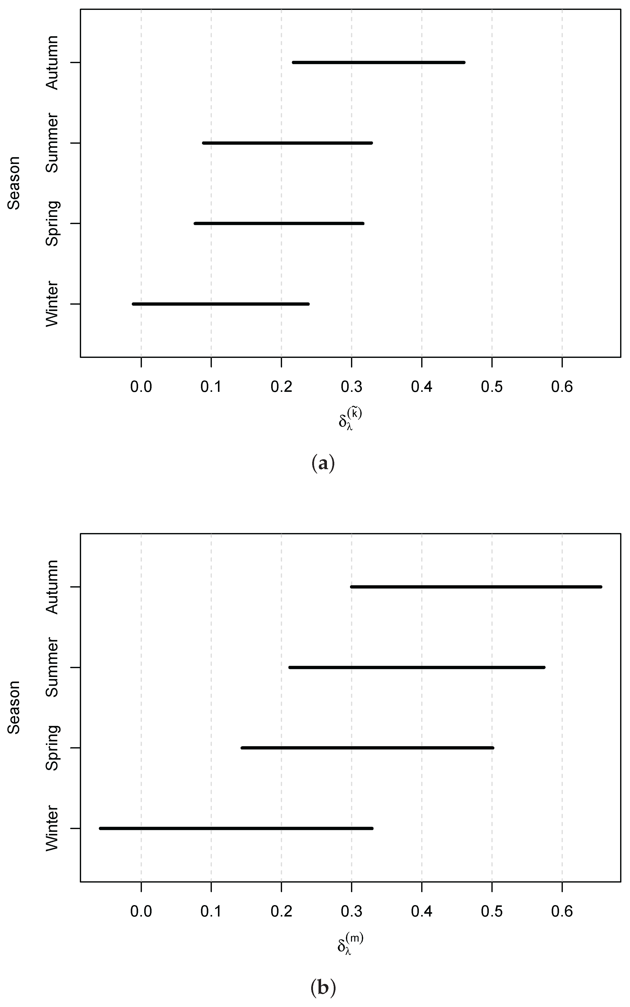
Next, we look at Models R 2 and R 4 with season-specific trend parameters for year and GMT, respectively. The trends at Newlyn are significant in both models, except for winter, whilst at Heysham, only the increasing trends in summer are significant. None of the seasonal trends are significant at Lowestoft, but we find a significant decreasing trend for spring in both models at Sheerness. As for Models R 1 and R 3 , we obtain a variety of results across sites; Newlyn has an increasing exceedance probability with year and GMT in all seasons. However, for Lowestoft and Sheerness, we obtain a mixture of positive and negative parameters throughout the year for both models. The confidence intervals for the four parameter estimates in Models R 2 and R 4 at Heysham, Lowestoft and Sheerness overlap, suggesting that there is not significant within-year variation in the long-term trend parameters so that the simpler Models R 1 and R 3 are sufficient. At Newlyn, this overlap is small (see Figure 3). Here, we find the greatest trend in autumn, which is not too concerning for extreme sea level estimation since the most extreme sea levels tend to occur in winter [15], but using Models R 1 and R 3 with common trend parameters across the year could overestimate the trends in winter, hence influencing sea level return level estimation.
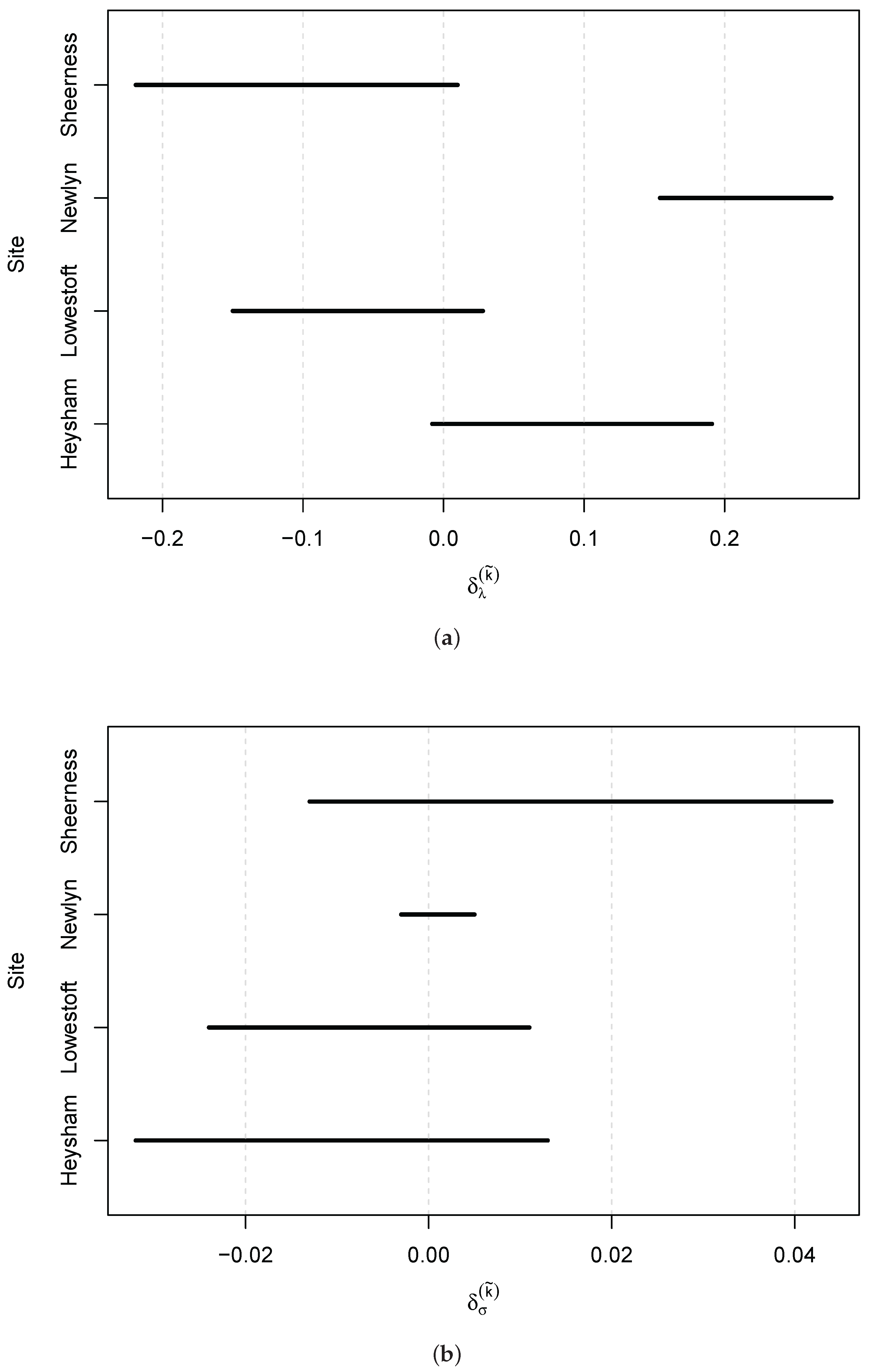
Next, we consider models for the scale parameter at each site individually (Models S0–4, introduced in Section 2.4). Table 3 shows the parameter estimates for each model, along with AIC and BIC scores. Models S 1 and S 3 have a single parameter denoting a common long-term trend across the year, but neither of these are an improvement on Model S 0 (without a long-term trend) at any site. All of the 95% confidence intervals for δ λ ( k ˜ ) or δ λ ( m ) estimates contain zero, suggesting these trends are not significant. If we ignore this uncertainty, the point estimates suggest small changes in the scale parameter. At Heysham and Lowestoft, our results show a decrease with both year and GMT, suggesting that the magnitude of extreme skew surge events are becoming smaller with anthropogenic climate change effects. In the 100 year period from 1920 to 2020 at Newlyn, the point estimate δ σ ( k ˜ ) corresponds to an increase in mean excesses (see expression (5)) of 2 mm (relative to a mean of 94 mm in 1920), whilst at Sheerness, in the years of observation from 1980 to 2016, this corresponds to an increase of 10 mm relative to a mean of 125 mm in 1980. Notice there is overlap in the parameter estimates for δ σ ( k ˜ ) and δ σ ( m ) across sites; in Section 3.4 we fit a similar model with these trend parameters common across sites (see Figure 4).
Models S 2 and S 4 have four additional parameters relative to Model S 0 , these denote a separate trend for each season with respect to year and GMT. AIC and BIC are still minimised by Model S 0 , except AIC scores for Heysham and Lowestoft, which favour Models S 2 and S 4 , respectively. However, the four confidence intervals overlap at each site, suggesting that a fixed trend within a year is sufficient. At Heysham, the overlap across all seasons is small but there is considerable overlap between winter and spring, with positive trend parameters, and likewise for summer and autumn with negative trend parameters for both models. If these trends were statistically significant, it would suggest that the magnitude of extreme skew surges is increasing with increases in GMT in December to April but decreasing for the rest of the year. Given the timing of the most extreme events, this could be important if statistically significant.

3.3. Return Level Estimation

Using Models S 0 (8) and R 4 () for the scale and rate parameters, respectively, we estimate sea level return levels from the annual maxima distribution in expression (11). Recall Model R 4 for the GPD rate parameter has a linear seasonal trend with respect to GMT in year k, denoted as m k . Solving
P ( M z | m k = m ) = 1 p
for p [ 0 , 1 ] gives us the level we expect the annual maxima M to exceed once every 1 / p years, on average, when the GMT covariate is fixed at some value m. We estimate return levels for temperatures in 1915, 2020 and for a year when the GMT anomaly value is 1 C higher than that in 2020; these correspond to anomalies of −0.19, 0.92 and 1.92 C, respectively.
Table 4 gives the sea level return level estimates for the 1100 and 10,000 year level at each site. These are relative to the mean sea level in 2017 since the linear mean sea level trend was removed when preprocessing the data, so these trends are in excess to those already observed in the mean or will occur as GMT increases. Return level estimates increase with temperature anomaly for all sites at all return periods. The 1 year level increases similarly (∼3–4cm) over the four sites, with the greatest difference of 10 cm observed at Heysham for the 10,000 year return level; this is a significant difference for coastal flood defence design. Return levels will be underestimated if the long-term trends in extreme skew surge occurrence are not accounted for and instead only estimated changes in mean sea level are used to update return level estimates. At Lowestoft, Newlyn and Sheerness, the 10,000 return level increases by 4, 3 and 2 cm, respectively, when GMT increases from −0.19 to 1.92 C. Therefore, even when some of the parameter estimates of Model R 4 for the seasonal GMT trend ( δ λ , s m for s = 1 , 2 , 3 , 4 ) were negative, the resulting return level estimates still increase with GMT. This outcome depends on which seasons have which trends. For annual maximum sea levels, it is only the winter and autumn trends that are influential. Although the seasonal changes seem non-homogeneous in the GPD model for extreme skew surges, our results show that when combined with tidal information, the sea level return levels exhibit much more consistent behaviour with GMT changes across sites.

3.4. Spatial Pooling

We present the results from pooling information across sites, for the long-term trend parameters, when refitting the models of Section 2.4. Before pooling information, we use the dependence measures discussed in Section 2.5 to check if it is reasonable to assume each pair of sites are independent in their extreme skew surge values. We estimate the dependence measures for the daily maximum observed skew surges and a standardised transformation of them to remove sources of within-year non-stationarity via mapping to uniform margins through the distribution function (7). The results are shown in Table 5. For most combinations of sites at lags t = 1 , 0 , 1 (days), the dependence is weak, except for Newlyn with each of the east coast sites where Kendall’s τ is near 0, whilst for Lowestoft and Sheerness this value is approximately 0.5. The effect of de-seasonalising the data (by transforming to uniform margins) has typically decreased dependence. With the exception of Lowestoft and Sheerness, it is not unreasonable to make an independence in extremes approximation for the data. We find χ ¯ < 1 for all pairs, giving evidence of asymptotic independence with weak dependence in the observed tails of the variables. The strongest dependence is found between Lowestoft and Sheerness at lag t = 0 . This is not surprising, since these sites are close in proximity, with extreme skew surges progressing south down the east coast through Lowestoft onto Sheerness. Therefore, they are highly likely to be affected by the same storms. Despite this pair of sites giving clear evidence of dependence, we continue under the belief that it is reasonable to assume skew surge daily maxima at all pairs of sites are sufficiently close to being independent for the purposes of spatial pooling.
Firstly, we focus on pooling information across sites regarding the long-term trend parameters with respect to year k and GMT m k for the rate parameter. Figure 4 shows there is considerable overlap in the confidence intervals for δ ^ λ ( k ˜ ) at Lowestoft and Sheerness; similarly, there is some overlap for Heysham and Newlyn. Although pooling information across randomly selected subsets of sites should be discouraged, here we note that the pairs of sites with similarities are on different coastlines, so we explore pooling over sites on the east coast (Lowestoft and Sheerness) and separately on the west coast (Heysham and Newlyn). Here, we consider refitting Models R 1 and R 3 (i.e., a fixed trend parameter within a year) with common trend parameters δ λ ( k ˜ ) and δ λ ( m ) between the pairs of sites. We obtain negative trend parameters δ ^ λ ( k ˜ ) = 0.084 ( 0.151 , 0.016 ) and δ ^ λ ( m ) = 0.070 ( 0.156 , 0.015 ) for Sheerness and Lowestoft, whilst at Newlyn and Heysham, we obtain statistically significant positive trend parameters δ ^ λ ( k ˜ ) = 0.180 ( 0.128 , 0.231 ) and δ ^ λ ( m ) = 0.285 ( 0.208 , 0.359 ) . Note that 95% confidence intervals are given in parentheses here. Both of these models are an improvement over the previous results, where a separate long-term trend parameter is used for each site; the model with a yearly trend parameter reduces AIC by 48 and the BIC by 0.5, whilst the model with a GMT parameter reduces AIC and BIC by 54 and 6, respectively. This highlights the importance of sharing information spatially.
There is also information to be gained from sharing spatial information about long-term trends in the scale parameter since there is considerable overlap in the confidence intervals for δ ^ σ ( k ˜ ) (see Figure 4) and δ ^ σ ( m ) (see Table 3). We refit the models of Section 2.4 for the scale parameter with common long-term trend parameters across sites, but neither parameter estimates are significant. We find that δ ^ σ ( k ˜ ) = 4.8 × 10 4 , corresponding to an increase in scale parameter of 0.48 mm over 1915–2020. For GMT δ ^ σ ( k ˜ ) = 0.0024 , i.e., a 24 mm decrease in scale parameter with a 1 C increase in temperature. Neither of these models improve the fit relative to having no long-term trends (in addition to those in the mean sea level), although the AIC scores are close. We also fit a model similar to that of Models S 2 and S 4 , so there is a common seasonal trend across sites, with respect to year and GMT, but we find that neither of these improve model fit. This agrees with our single-site results of Section 3.2 where we found no evidence of changes in the magnitude of extreme skew surge events with respect to year or GMT.

4. Discussion

We have presented a framework to investigate the effects of anthropogenic climate change on extreme skew surges as any increases in the magnitude or frequency in these events can have catastrophic consequences if not included in extreme sea level estimation for coastal flood defence design. These trends can be different to those observed in the main body of the data, such as mean sea level rise. We use year and GMT as covariates in our statistical model for extreme event occurrence, building on a model developed by [15] that accounts for seasonality and skew surge–peak tide dependence. Recall that our results are relative to the mean sea level trend in 2017, so this would need to be added onto any sea level return level estimates when used in practice. We show that there is evidence of an increase in the probability of an extreme skew surge event with GMT increases at Heysham and Newlyn, but evidence of both increases and decreases in the likelihood of these events at Lowestoft and Sheerness across the year. We do not find any significant changes in the magnitude of extreme skews surges, i.e., in the scale parameter, and hence in the mean of the skew surge excesses of the threshold. Accounting for seasonal changes in extreme skew surge occurrence with GMT in sea level return level estimation shows that return levels increase with GMT. For a 2.1 C increase in GMT, the 10,000 year return levels increased by 10, 4, 3 and 2 cm at Heysham, Lowestoft, Newlyn and Sheerness, respectively. The ideas presented in this paper could be applied to more locations but also to other environmental variables to investigate trends in extreme values.
We demonstrate the advantages of pooling information across sites, although this is only primarily illustrative since we consider just four sites here. There are 44 sites on the UK National Tide Gauge Network where this methodology could be extended. It would be interesting to apply our methodology within a spatial framework, for example, in regional frequency analysis where sites in a homogeneous region not only have a common shape parameter but also common long-term trends due to anthropogenic climate change.
Skew surges are also believed to change over decadal time scales with climate indices. For example, the North Atlantic Oscillation index (NAO) describes such time scale changes in regional weather systems, so it is believed to impact storm surges and thus skew surge. Ref. [39] find a negative correlation between storm surge and air pressure patterns, using NAO. It would be interesting to explore how adding an NAO covariate into the GPD for extreme skew surges would change model fit.

Author Contributions

Conceptualization, D.E.S.; methodology, E.D. and J.A.T.; software, E.D.; validation, J.A.T.; formal analysis, E.D.; investigation, E.D.; resources, J.A.T.; data curation, E.D.; writing—original draft preparation, E.D.; writing—review and editing, E.D., J.A.T. and D.E.S.; visualization, E.D.; supervision, J.A.T. and D.E.S.; project administration, J.A.T.; funding acquisition, J.A.T. and D.E.S. All authors have read and agreed to the published version of the manuscript.

Funding

This paper is based on work completed while Eleanor D’Arcy was part of the EPSRC funded STOR-i centre for doctoral training (EP/S022252/1).

Institutional Review Board Statement

Not applicable.

Informed Consent Statement

Not applicable.

Data Availability Statement

Data are from the UK National Tide Gauge Network, owned and operated by the Environment Agency and obtained from the British Oceanographic Data Centre (BODC): https://www.bodc.ac.uk/data/hosted_data_systems/sea_level/uk_tide_gauge_network/processed/, accessed on 1 July 2022.

Acknowledgments

Thanks to Jenny Sansom of the Environment Agency and Joanne Williams of National Oceanography Centre for providing the data.

Conflicts of Interest

The authors declare no conflict of interest.

References

  1. Zsamboky, M.; Fernández-Bilbao, A.; Smith, D.; Knight, J.; Allan, J. Impacts of Climate Change on Disadvantaged UK Coastal Communities; Joseph Rowntree Foundation: York, UK, 2011; pp. 1–63. [Google Scholar]
  2. Seneviratne, S.; Nicholls, N.; Easterling, D.; Goodess, C.M.; Kanae, S.; Kossin, J.; Luo, Y.; Marengo, J.; McInnes, K.; Rahimi, M.; et al. Changes in climate extremes and their impacts on the natural physical environment. In Managing the Risks of Extreme Events and Disasters to Advance Climate Change Adaptation; A Special Report of Working Groups I and II of the Intergovernmental Panel on Climate Change, (IPCC); Field, C.B., Barros, V., Stocker, T.F., Qin, D., Dokken, D.J., Ebi, K.L., Mastrandrea, M.D., Mach, K.J., Plattner, G.K., Allen, S.K., et al., Eds.; Cambridge University Press: Cambridge, UK; New York, NY, USA, 2012; Volume 3, pp. 109–230. [Google Scholar]
  3. Seneviratne, S.I.; Zhang, X.; Adnan, M.; Badi, W.; Dereczynski, C.; Di Luca, A.; Ghosh, S.; Iskandar, I.; Kossin, J.; Lewis, S.; et al. Weather and Climate Extreme Events in a Changing Climate. In Climate Change 2021: The Physical Science Basis; Contribution of Working Group I to the Sixth Assessment Report of the Intergovernmental Panel on Climate, Change; Masson-Delmotte, V., Zhai, P., Pirani, A., Connors, S.L., Péan, C., Berger, S., Caud, N., Chen, Y., Goldfarb, L., Gomis, M.I., et al., Eds.; Cambridge University Press: Cambridge, UK; New York, NY, USA, 2021; Volume 11, pp. 1513–1766. [Google Scholar] [CrossRef]
  4. Morice, C.P.; Kennedy, J.J.; Rayner, N.A.; Winn, J.; Hogan, E.; Killick, R.; Dunn, R.; Osborn, T.; Jones, P.; Simpson, I. An updated assessment of near-surface temperature change from 1850: The HadCRUT5 data set. J. Geophys. Res. Atmos. 2021, 126, e2019JD032361. [Google Scholar] [CrossRef]
  5. Egbert, G.D.; Ray, R.D. Tidal prediction. J. Mar. Res. 2017, 75, 189–237. [Google Scholar] [CrossRef]
  6. Pugh, D.; Woodworth, P. Sea-Level Science: Understanding Tides, Surges, Tsunamis and Mean Sea-Level Changes; Cambridge University Press: Cambridge, UK, 2014. [Google Scholar]
  7. Williams, J.; Horsburgh, K.J.; Williams, J.A.; Proctor, R.N. Tide and skew surge independence: New insights for flood risk. Geophys. Res. Lett. 2016, 43, 6410–6417. [Google Scholar] [CrossRef]
  8. Howard, T.; Williams, S.D.P. Towards using state-of-the-art climate models to help constrain estimates of unprecedented UK storm surges. Nat. Hazards Earth Syst. Sci. 2021, 21, 3693–3712. [Google Scholar] [CrossRef]
  9. Woodworth, P.L.; Player, R. The Permanent Service for Mean Sea Level: An Update to the 21st Century. J. Coast. Res. 2003, 19, 287–295. [Google Scholar]
  10. Wahl, T.; Haigh, I.D.; Woodworth, P.L.; Albrecht, F.; Dillingh, D.; Jensen, J.; Nicholls, R.J.; Weisse, R.; Wöppelmann, G. Observed mean sea level changes around the North Sea coastline from 1800 to present. Earth-Sci. Rev. 2013, 124, 51–67. [Google Scholar] [CrossRef]
  11. Calafat, F.M.; Wahl, T.; Tadesse, M.G.; Sparrow, S.N. Trends in Europe storm surge extremes match the rate of sea-level rise. Nature 2022, 603, 841–845. [Google Scholar] [CrossRef]
  12. Weiss, J.; Bernardara, P. Comparison of local indices for regional frequency analysis with an application to extreme skew surges. Water Resour. Res. 2013, 49, 2940–2951. [Google Scholar] [CrossRef]
  13. Wong, T.E.; Sheets, H.; Torline, T.; Zhang, M. Evidence for Increasing Frequency of Extreme Coastal Sea Levels. Front. Clim. 2022, 4. [Google Scholar] [CrossRef]
  14. Woodworth, P.L.; Menéndez, M.; Roland Gehrels, W. Evidence for century-timescale acceleration in mean sea levels and for recent changes in extreme sea levels. Surv. Geophys. 2011, 32, 603–618. [Google Scholar] [CrossRef] [Green Version]
  15. D’Arcy, E.; Tawn, J.A.; Joly, A.; Sifnioti, D.E. Accounting for Seasonality in Extreme Sea Level Estimation. arXiv 2022, arXiv:2207.09870. [Google Scholar] [CrossRef]
  16. Coles, S.G. An Introduction to Statistical Modeling of Extreme Values; Springer: London, UK, 2001. [Google Scholar]
  17. Environment Agency. Coastal Flood Boundary Conditions for the UK: Update 2018. Technical Summary Report. 2018. Available online: https://environment.data.gov.uk/dataset/6e856bda-0ca9-404f-93d7-566a2378a7a8 (accessed on 1 October 2021).
  18. Leadbetter, M.; Lindgren, G.; Rootzén, H. Extremes and Related Properties of Random Sequences and Processes; Springer: New York, NY, USA, 1983. [Google Scholar]
  19. Ferro, C.A.T.; Segers, J. Inference for clusters of extreme values. J. R. Stat. Soc. Ser. B 2003, 65, 545–556. [Google Scholar] [CrossRef]
  20. Smith, R.L.; Weissman, I. Estimating the extremal index. J. R. Stat. Soc. Ser. B 1994, 56, 515–528. [Google Scholar] [CrossRef]
  21. Ledford, A.W.; Tawn, J.A. Diagnostics for dependence within time series extremes. J. R. Stat. Soc. Ser. B 2003, 65, 521–543. [Google Scholar] [CrossRef]
  22. Smith, R.L.; Tawn, J.A.; Coles, S.G. Markov chain models for threshold exceedances. Biometrika 1997, 84, 249–268. [Google Scholar] [CrossRef]
  23. Fawcett, L.; Walshaw, D. Improved estimation for temporally clustered extremes. Environmetrics 2007, 18, 173–188. [Google Scholar] [CrossRef]
  24. Graff, J. Concerning the recurrence of abnormal sea levels. Coast. Eng. 1978, 2, 177–187. [Google Scholar] [CrossRef]
  25. Coles, S.G.; Heffernan, J.; Tawn, J.A. Dependence Measures for Extreme Value Analyses. Extremes 1999, 2, 339–365. [Google Scholar] [CrossRef]
  26. Tawn, J.A. An extreme-value theory model for dependent observations. J. Hydrol. 1988, 101, 227–250. [Google Scholar] [CrossRef]
  27. Dixon, M.J.; Tawn, J.A. The effect of non-stationarity on extreme sea-level estimation. J. R. Stat. Soc. Ser. C 1999, 48, 135–151. [Google Scholar] [CrossRef]
  28. Pugh, D.; Vassie, J. Extreme sea levels from tide and surge probability. Coast. Eng. 1978, 16, 911–930. [Google Scholar]
  29. Tawn, J.A. Estimating probabilities of extreme sea-levels. J. R. Stat. Soc. Ser. C 1992, 41, 77–93. [Google Scholar] [CrossRef]
  30. Batstone, C.; Lawless, M.; Tawn, J.A.; Horsburgh, K.; Blackman, D.; McMillan, A.; Worth, D.; Laeger, S.; Hunt, T. A UK best-practice approach for extreme sea-level analysis along complex topographic coastlines. Ocean. Eng. 2013, 71, 28–39. [Google Scholar] [CrossRef]
  31. Baranes, H.; Woodruff, J.; Talke, S.; Kopp, R.; Ray, R.; DeConto, R. Tidally driven interannual variation in extreme sea level frequencies in the Gulf of Maine. J. Geophys. Res. Ocean. 2020, 125, e2020JC016291. [Google Scholar] [CrossRef]
  32. Eastoe, E.F.; Tawn, J.A. Modelling non-stationary extremes with application to surface level ozone. J. R. Stat. Soc. Ser. C 2009, 58, 25–45. [Google Scholar] [CrossRef]
  33. Northrop, P.J.; Attalides, N.; Jonathan, P. Cross-validatory extreme value threshold selection and uncertainty with application to ocean storm severity. J. R. Stat. Soc. Ser. C 2017, 66, 93–120. [Google Scholar] [CrossRef]
  34. Wadsworth, J.L. Exploiting Structure of Maximum Likelihood Estimators for Extreme Value Threshold Selection. Technometrics 2016, 58, 116–126. [Google Scholar] [CrossRef]
  35. Davison, A.C.; Padoan, S.A.; Ribatet, M. Statistical modeling of spatial extremes. Stat. Sci. 2012, 27, 161–186. [Google Scholar] [CrossRef]
  36. Dixon, M.J.; Tawn, J.A.; Vassie, J.M. Spatial modelling of extreme sea-levels. Environmetrics 1998, 9, 283–301. [Google Scholar] [CrossRef]
  37. Huser, R.; Genton, M.G. Non-stationary dependence structures for spatial extremes. J. Agric. Biol. Environ. Stat. 2016, 21, 470–491. [Google Scholar] [CrossRef]
  38. Southworth, H.; Heffernan, J.E.; Metcalfe, P.D. Texmex: Statistical Modelling of Extreme Values, R Package Version 2.4.8. 2020. Available online: https://cran.r-project.org/web/packages/texmex (accessed on 1 July 2022).
  39. Araújo, I.B.; Pugh, D.T. Sea levels at Newlyn 1915–2005: Analysis of trends for future flooding risks. J. Coast. Res. 2008, 24, 203–212. [Google Scholar] [CrossRef]
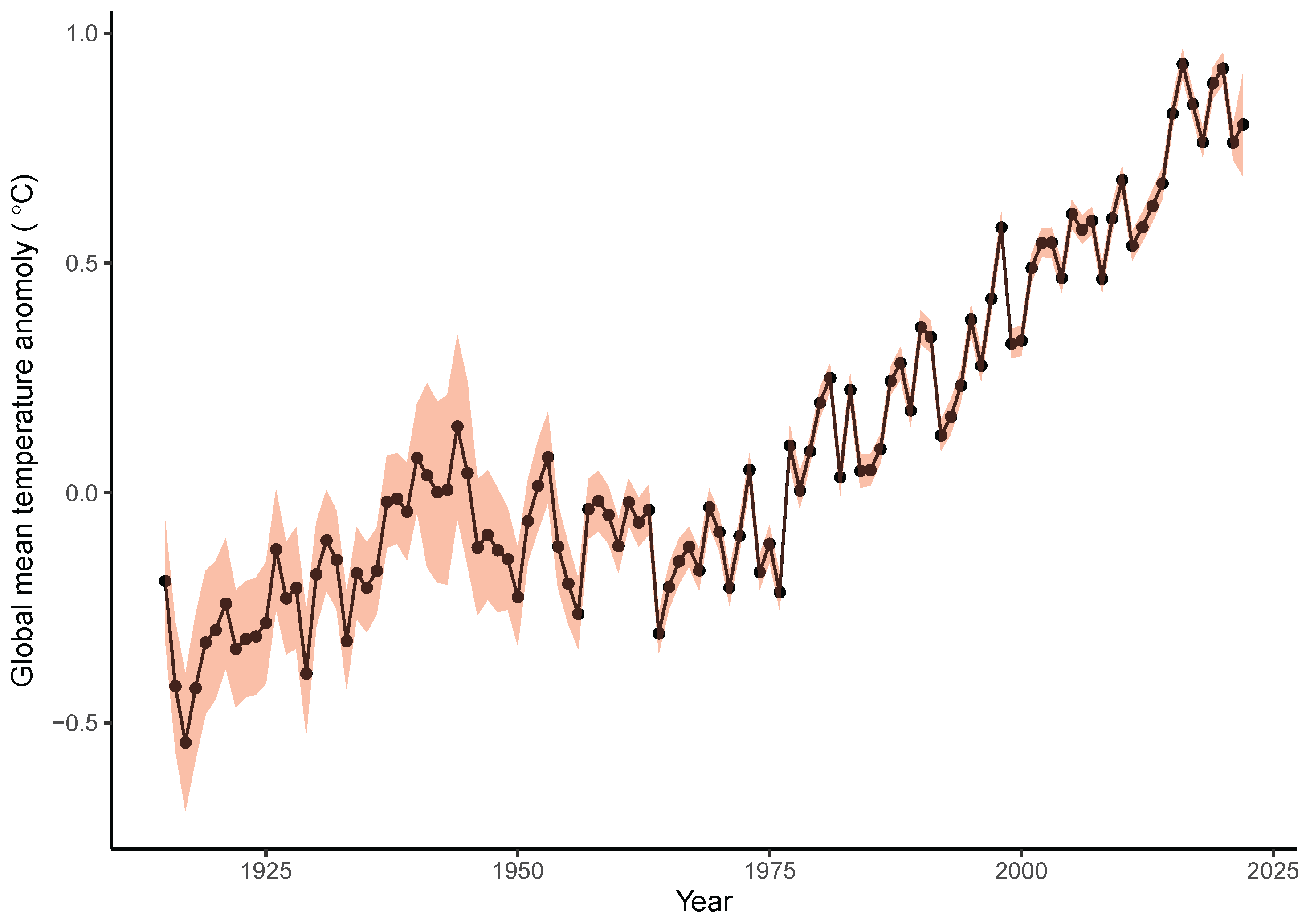
Figure 1. Global mean temperature anomalies from the HadCRUT5 dataset in 1915–2020, relative to the period 1961–1990, with associated uncertainties in red [4].
Water 14 02956 g001
Figure 2. Histograms of (a) Δ λ ( k ˜ ) over 100 years and (b) Δ λ ( m ) with a 1 C increase in GMT, as percentages, for all day d and peak tide x combinations at each site.
Water 14 02956 g002
Figure 3. Confidence intervals for parameter estimates: (a) δ ^ λ , s ( k ˜ ) and (b) δ ^ λ , s ( m ) at Newlyn for s = 1 , 2 , 3 , 4 denoting winter, spring, summer and autumn, respectively.
Water 14 02956 g003
Figure 4. Confidence intervals for parameter estimates δ ^ λ ( k ˜ ) (a) and δ ^ σ ( k ˜ ) (b) for all sites.
Water 14 02956 g004
Table 1. Location (latitude and longitude), observation period, percentage of missing data, highest astronomical tide (HAT) in metres and estimated mean sea level (MSL) trend in mm/yr for Heysham, Lowestoft, Newlyn and Sheerness.
LocationObservation Period% MissingHAT (m)MSL Trend (mm/yr)
Heysham 54 . 03 N,
2 . 92 W
1964–20161710.721.52
Lowestoft 2 . 47 N,
1 . 75 E
1964–202042.922.27
Newlyn 50 . 10 N,
5 . 54 W
1915–2016176.101.73
Sheerness 51 . 45 N,
0 . 74 E
1980–2016196.261.81
Table 2. Parameter estimates for the Models R 1 R 4 with AIC and BIC scores for each model fit at each site (including Model R 0 ). The minimum AIC and BIC scores are highlighted in red and blue, respectively, for each site. The 95% confidence intervals are given in parentheses for parameter estimates.
HeyshamLowestoftNewlynSheerness
Model R 0
AIC12,234.2115,312.0824,498.779286.58
BIC12,275.8915,354.8824,543.939326.94
Model R 1
δ λ ( k ˜ ) 0.091 (−0.008, 0.191)−0.061 (−0.150, 0.028)0.215 (0.154,0.276)−0.114 (−0.219, −0.010)
AIC12,232.8915,312.2624,453.129283.96
BIC12,282.9115,363.6124,507.319332.40
Model R 2
δ λ , 1 ( k ˜ ) 0.161 (−0.033, 0.335)0.063 (−0.106, 0.232)0.114 (−0.011, 0.238)−0.032 (−0.228, 0.164)
δ λ , 2 ( k ˜ ) 0.034 (−0.161, 0.230)−0.141 (−0.322, 0.040)0.197 (0.077, 0.316)−0.250 (−0.468, −0.032)
δ λ , 3 ( k ˜ ) 0.207 (0.013, 0.400)−0.094 (−0.266, 0.078)0.209 (0.089, 0.328)−0.189 (−0.405, 0.026)
δ λ , 4 ( k ˜ ) −0.047 (−0.261, 0.167)−0.081 (−0.264, 0.102)0.338 (0.217, 0.460)−0.021 (−0.221, 0.178)
AIC12,235.3015,315.2924,452.529286.48
BIC12,310.3215,392.3324,533.809359.14
Model R 3
δ λ ( m ) 0.204 (0.074, 0.334)−0.012 (−0.12, 0.427)0.336 (0.245, 0.427)−0.164 (−0.304, −0.024)
AIC12,227.1415,314.0424,451.349283.20
BIC12,277.1615,365.3924,505.539331.64
Model R 4
δ λ , 1 ( m ) 0.256 (−0.002, 0.514)0.103 (−0.107, 0.312)0.135 (−0.058, 0.329)−0.079 (−0.340, 0.181)
δ λ , 2 ( m ) 0.111 (−0.143, 0.365)−0.067 (−0.282, 0.149)0.322 (0.144, 0.501)−0.374 (−0.672, −0.076)
δ λ , 3 ( m ) 0.416 (0.167, 0.665)−0.048 (−0.259, 0.163)0.393 (0.212, 0.574)−0.273 (−0.568, 0.022)
δ λ , 4 ( m ) 0.010 (−0.274, 0.293)−0.040 (−0.262, 0.182)0.478 (0.300, 0.655)0.008 (−0.253, 0.269)
AIC12,227.9215,318.4924,450.279284.69
BIC12,302.9415,395.5324,531.569357.34
Table 3. Parameter estimates for the Models S1-4 with AIC and BIC scores for each model fit at each site (including Model S 0 ). The minimum AIC and BIC scores are highlighted in red and blue, respectively, for each site. The 95% confidence intervals are given in parentheses for parameter estimates.
HeyshamLowestoftNewlynSheerness
Model S 0
AIC−3091.53−3672.07−10,152.63−2974.317
BIC−3064.77−3644.20−10,122.42−2948.854
Model S 1
δ σ ( k ˜ ) −0.009 (−0.032, 0.013)−0.006 (−0.024, 0.011)0.001 (−0.003, 0.005)0.016 (−0.013, 0.044)
AIC−3088.558−3670.55−10,150.80−2973.05
BIC−3056.448−3637.11−10,114.54−2942.50
Model S 2
δ 1 ( k ˜ ) 0.022 (−0.034, 0.078)−0.041 (−0.090, 0.007)0.004 (−0.009, 0.016)0.023 (−0.032, 0.078)
δ 2 ( k ˜ ) 0.022 (−0.014, 0.059)−0.030 (−0.055, −0.006)0.006 (−0.002, 0.014)−0.001 (−0.036, 0.035)
δ 3 ( k ˜ ) −0.025 (−0.051, 0.001)0.012 (−0.010, 0.034)−0.003 (−0.009, 0.003)0.023 (−0.010, 0.055)
δ 4 ( k ˜ ) −0.035 (−0.079, 0.008)−0.015 (−0.053, 0.023)0.001 (−0.008, 0.011)0.008 (−0.039, 0.054)
AIC−3095.28−3674.12−10,146.27−2971.19
BIC−3047.12−3623.96−10,091.89−2925.36
Model S 3
δ σ ( m ) −0.011 (−0.033, 0.011)−0.008 (−0.026, 0.009)−0.001 (−0.008, 0.006)0.006 (−0.020, 0.032)
AIC−3088.42−3670.90−10,149.07−2972.43
BIC−3056.32−3637.46−10,112.82−2941.87
Model S 4
δ 1 ( m ) 0.036 (−0.027, 0.099)−0.050 (−0.105, 0.004)−0.0003 (-0.021, 0.020)0.025 (-0.042, 0.091)
δ 2 ( m ) 0.029 (−0.012, 0.070)−0.037 (−0.061, −0.012)0.005 (−0.008, 0.018)−0.015 (−0.054, 0.023)
δ 3 ( m ) −0.027 (−0.054, −0.00009)0.017 (−0.006, 0.039)−0.003 (−0.013, 0.006)0.013 (−0.018, 0.045)
δ 4 ( m ) −0.030 (−0.081, 0.021)−0.024 (−0.066, 0.017)−0.005 (−0.021, 0.010)−0.006 (−0.053, 0.040)
AIC−3093.73−3677.95−10145.39−2970.79
BIC−3045.56−3627.79−10091.01−2924.96
Table 4. Estimates of the 1100 and 10,000 year sea level return levels (in metres), relative to the mean sea level in 2017, using Models R 4 and S 0 for the GPD rate and scale parameters, respectively, for skew surges with GMT as a fixed covariate equal to anomalies of −0.19 C (as in 1915), 0.92 C (as in 2020) and 1.92 C.
HeyshamLowestoftNewlynSheerness
110010,000110010,000110010,000110010,000
−0.19  C10.6111.5212.453.474.605.816.076.556.946.417.177.98
−0.92  C10.6311.5612.503.494.615.836.096.576.956.427.187.99
−1.92  C10.6511.6012.553.504.635.856.116.606.976.447.198.00
Table 5. Kendall’s τ , χ and χ ¯ measures of dependence for daily maximum skew surge observations at pairs of sites. We show the dependence over lags −1 (LHS site is 1 day behind RHS), 0 and 1 (LHS site is 1 day ahead of RHS); in bold we show the largest dependence over these lags. χ and χ ¯ are measures of extremal dependence for exceedances of the 0.95 quantile.
Heysham–LowestoftHeysham–NewlynHeysham–SheernessLowestoft–NewlynLowestoft–SheernessNewlyn–Sheerness
lag101101101101101101
Observations
τ 0.1330.1600.3090.2870.3220.2590.1530.1490.2980.0890.0400.0340.1550.5100.2380.1370.1680.196
χ 0.0950.1290.2700.1270.1450.0760.0920.1110.2590.017000.1450.5090.2000.0540.0770.121
χ ¯ 0.2000.2510.4240.2490.2760.1600.1950.2240.4120.040−0.018−0.0550.2740.6450.3440.1200.1580.237
Transform to Uniform (0,1)
τ 0.1030.1300.2890.2850.3180.2440.1080.1020.2620.0860.0360.0280.1430.5230.2280.1390.1730.200
χ 0.0260.0400.1800.1030.1220.0530.0560.0360.1730000.0950.4940.1740.0030.0160.050
χ ¯ 0.0690.1000.3210.2150.2360.1140.1230.0840.313−0.012−0.107−0.1340.1980.6340.3160.0030.0350.114
Publisher’s Note: MDPI stays neutral with regard to jurisdictional claims in published maps and institutional affiliations.