Article

Effects of Slide Shape on Impulse Waves Generated by a Subaerial Solid Slide

Department of Civil Engineering, National Taiwan University, Taipei 10617, Taiwan
*
Author to whom correspondence should be addressed.
Water 2022, 14(17), 2643; https://doi.org/10.3390/w14172643
Submission received: 5 July 2022 / Revised: 10 August 2022 / Accepted: 24 August 2022 / Published: 27 August 2022
(This article belongs to the Special Issue Marine Environmental Research)

Abstract

:
We review several historical landslide tsunami events and perform a set of numerical experiments to investigate the particular effects of slide shape on impulsive waves generated by a subaerial solid slide. The computational model is based on OpenFOAM, which solves 2D RANS formulations with a volume of fluid method used to capture the air–water interface. We consider triangular prism shaped solid slides in our numerical experiments and introduce a slide shape parameter σ to describe the front face steepness of the slide. Observations from the experiments reveal that slide shape can have significant impacts on the characteristics of impulsive waves, such as maximum wave amplitude and its location, impact energy conversion rate, and the amplitude ratio between the first wave crest and the second crest in the leading wave group. In particular, the maximum wave amplitude is inversely proportional to σ ; the impact energy conversion ratio decays exponentially with σ ; and the wave period is almost independent of σ .

1. Introduction

Surface water waves of considerable wave height generated as a consequence of abrupt impacts caused by either subaerial or submarine landslides have been observed globally at continental margins and in more confined coastal regions such as bays, lakes, and reservoirs [1]. Theoretical analysis [2] and physical modeling [3] of landslide-generated waves have demonstrated that the volume of landslide possesses dominant importance in the production of this type of impulsive waves. In other words, a landslide of a considerable volume has the tendency to generate exceedingly large waves, commonly known as landslide tsunamis, which can pose significant disaster risks to human life and cause huge amounts of economic damage in densely populated coastal communities [4]. For example, activated by a Mw 8.3 earthquake, the 1958 Lituya Bay Tsunami that recorded an exceptional maximum run-up height of 524 m was induced when an estimated 3 × 10 7 m 3 volume of slide material, consisting mainly of rock and ice, fell into the narrow Gilbert Inlet at the head of Lituya Bay, a fjord located on the long stretch coast of southeastern Alaska [5]. We note that the slide volume was calculated based on the rough estimation of the dimensions through the comparison of the aerial photographs taken before and after the earthquake, and the maximum tsunami run-up was determined with the help of the glacial trimlines depicted by the photographic evidence [6]. More recently, in the nearby Icy Bay, a massive landslide that generated a significant local tsunami with a maximum run-up height of 193 m and an inundation area over 20 km 2 also occurred in October 2015 [7]. Using the LiDAR data collected during the post-tsunami field survey, the slide volume in the 2015 event was calculated to be in the order of 75 million m 3 and about two-thirds of the evacuated volume flowed into the Taan Fjord, the eastern arm of Icy Bay [8]. Despite the aforementioned 1958 and 2015 mega tsunamis sharing the same wave generation mechanism, i.e., they were both set in motion by the massive subaerial rock slides fell into the narrow parts of the fjords, the major triggers for these two landslide hazards were quite different from each other [6,7]. The slope failure that eventually generated the 1958 landslide tsunami was mainly associated with the energetic strike-slip earthquake struck on the Fairweather Fault, which runs through the head of the T-shaped Lituya Bay, with the epicenter only 13 miles southeast of the estuary head [6,9]. As for the 2015 event, it has been suggested that while both the mild ground motion induced by a distant Mw 4.1 earthquake centered about 500 km away and the rise of groundwater table due to heavy rainfall may have contributed to the slope failure, the most significant contribution to the landslide was the glacial retreat and ice melting as a consequence of the recent rapid warming, which altered the stress behaviors in the adjacent fjord slopes [7,8]. We remark that, because of their distinct geomorphological features of being long, narrow, and over-deepened valleys bounded by steep mountain walls, glacial fjords on the coasts of Alaska pose a significant risk for landslide tsunamis [10]. In the past century, we have witnessed four tsunami events with run-up of at least 60 m resulting from subaerial landslides into fjords in this region [7]. Similar to Alaska’s glacially sculpted coastlines that are susceptible to tsunami hazards, in Norway and Greenland, many glacial fjords with long and steep mountainsides and deep waters are also favorable locations for the efficient generation of destructive landslide tsunamis [7,10,11]. In fact, frequent landslides along the Norwegian fjords have resulted in several tsunami hazards since the turn of the twentieth century [11,12]. For instance, in the notorious 1934 Tafjord accident, about 2 million m 3 of rock tumbled down into the roughly 10 km long, 1 km wide fjord from the mountain rock face at a height of 730 m [13]. In a matter of minutes, the landslide-generated tsunamis that reached a maximum run-up height of 62 m crashed the downstream as well as upstream villages and claimed forty casualties while the waves funneled through the fjord in both directions [7,13,14]. On the other hand, in Greenland, there were two destructive tsunamis caused by the subaerial landslides into fjords during the past two decades, namely the 2000 event in Paatuut [15] and the 2017 deadly tsunami in Karrat Fjord [16]. We note that in these two landslides, the elevations where the main body of the slide material situated at were both about 1000 m and the volume of the slide and the resulting maximum tsunami run-up height for the 2000 landslide and tsunami were around 30 million m 3 and 50 m, respectively, whereas in the 2017 event the volume was 58 million m 3 and the run-up reached 90 m [7,15,16].
Landslide tsunamis occurring in relatively enclosed water bodies like lakes and reservoirs can often be more destructive and fatal since most of the tsunami wave energy is trapped within the confined regions [17]. Furthermore, in the case of tsunamis in reservoirs, the dam-breach floods due to tsunami-induced dam failures undoubtedly aggravate the disasters [18]. In the past century, the deadliest landslide tsunamis in lakes or reservoirs are exemplified by two major events in Norway’s Lake Lovatnet, i.e., the Loen accidents in 1905 and 1936 that killed a combined 134 people [19], the 1971 Yanahuin Lake disaster in Peru causing hundreds of fatalities [20], and the 1963 Vajont Dam catastrophe in Italy that was responsible for more than 2000 deaths [21]. The associated maximum run-up heights in the Lake Lovatnet and Yanahuin Lake events were 74 m and 30 m, respectively, and the corresponding volumes of the mobilized material were in the order of 10 5 to 10 6 m 3 , which were a few orders of magnitude less than the volumes in those previously discussed tsunamis hazards that have occurred in glacial fjords. Concerning the 1963 Vajont Dam disaster, during the filling stages of the reservoir formed by the then newly completed dam, a slide mass of approximately 300 million m 3 collapsed into the reservoir, generating an enormous tsunami that overtopped the 262 m high thin arch dam by up to 245 m in mere minutes [22]. Surprisingly, the concrete dam remained intact but the downstream villages were wiped clean by the overtopping flood [18]. The major cause of the catastrophic slope failures was the geologically unstable slopes triggered by the rapid change of the soil condition due to the repeated filling and drawdown cycles of the reservoir [23]. It is generally agreed the tragedy of Vajont was the result of insufficient geological investigations for site selection and even worse the poor decision by the project management and authority to ignore the early signs and warnings of the ultimate disaster [24].
Destructive tsunamis generated by submarine landslides are also not uncommon, as evidenced by three exemplary events in the past few decades, killing around 5000 people altogether, namely the 1998 Papua New Guinea disaster [25], the 2018 tsunami in Indonesia’s Palu Bay [26], and the 2018 Anak Krakatau Tsunami in the Sunda Straits of Indonesia [27]. Candidate deposits of submarine landslides have been found ubiquitously in coastal environments and tsunamigenic landslides may occur on most continental margins in a broad range of geologic and bathymetric settings, even along very gentle seabed slopes [28]. Historical evidences have suggested that submarine landslide tsunamis are often triggered by tectonic earthquakes, even small or distance earthquakes [2], or volcanically-induced [27]. For instance, the 1998 Papua New Guinea and 2018 Palu Bay tsunamis were earthquake-linked [25,26], while the 2018 Anak Krakatau event occurred along the volcano flank [27]. Since it is difficult to monitor or observe any slide event in the subsea realm, submarine landslide tsunamis often come in surprise and in turn cause more extreme consequences to the unprepared society [2,29]. A mounting example is the devastating 1964 disaster occurred in the Prince William Sound region of Alaska, where the majority of casualties was claimed by the tsunami waves generated as a result of an earthquake-induced local submarine landslide [30].
Compared to more frequent transoceanic tsunamis excited by seismic dislocations, landslide tsunamis tend to be more localized, with exceptionally large run-ups along limited coastal extents, but insignificant far-field impacts because the volume of displaced water is still too small to provide sufficient energy for sustaining tsunami propagation over long distances [31,32]. The generation mechanism of landslide tsunamis also differs dramatically from that of major earthquake tsunamis in the sense that landslide-generated tsunamis spread radially from the source region whereas earthquake tsunamis radiate in both directions perpendicular to the fault lines [29]. While we have been long aware of potential major tsunamis being generated by landslides, perhaps challenged by the devastating 1998 Papua New Guinea Tsunami, significantly more efforts have since been invested to better understand the generation, propagation and run-up of waves from slides, as to equal what we know about earthquake-induced tsunamis [33,34]. Among others, some representative studies reported in the literature include the most direct physical modeling of the near-field and far-field features of waves generated by either subaerial [35] or submarine landslides [36], analytical predictions for the propagation and run-up of landslide tsunamis in idealized settings [37,38], and computational models based on classical linear wave formulations for predicting waves generated by a submarine solid block moving horizontally in a constant depth [2], the depth-integrated long wave equations reproducing the 1998 Papua New Guinea Tsunami [25], the LES (large eddy simulation) approach to study the waves generated by a sliding solid and the associated wave run-up and draw-down on a sloping beach [34], and the multi-phase flow framework to examine the impulsive waves due to the collapse of a steep slope into a water body [39]. The physics behind the life of a landslide tsunami are rather complicated. However, lessons learned from historical events have suggested that the knowledge of leading tsunami waves is especially valuable for tsunami hazard mitigation planning [40]. In particular, the wave height of leading waves is a crucial element, since it can be used to predict the terminal effects of maximum tsunami run-up height [41]. Previous studies suggested that the wave characteristics of impulsive waves generated by subaerial landslides depend heavily on slide impact velocity, often represented by its centroid velocity, and landslide volume while other parameters, such as the slide shape, play a marginal role [35,42,43]. Regarding waves generated by submarine landslides, the dominant factors are bed slope angle, slide initial submergence, and thickness of the slide, with slide length only having a milder effect [36,44,45].
In all, it is reasonable to say that the generation of landslide impulsive waves is controlled by both the effects of initial slide impact quantified mainly by the slide centroid velocity and the bed slope and the slide volume incorporating the combined influences of slide thickness and length. The actual slide shape, on the other hand, has only an insignificant impact. Along this line, empirical formulas for wave amplitudes, based on either laboratory data [35,36,43,45] or numerical simulations [44], have been established. Using this wave amplitude estimation as an input for the existing run-up formulas available in literature [41,46], we will be able to obtain a swift evaluation on the maximum run-up height for landslide tsunamis. However, a recent study on run-up of non-decaying dam-break bores [47] demonstrated that the front face of incoming waves actually controls the maximum run-up height. In other words, if we consider different transient waves with distinct wave shapes but sharing the same wave height, the one with the steepest front face will yield the largest run-up height. In the literature, canonical wave models derived from classical wave theories have often been used to describe the wave shape of landslide generated waves, i.e., these impulsive waves are simply classified as stokes-type, cnoidal-type, solitary-type, or bore-type waves [35,48,49]. To facilitate a clear understanding of the parameters controlling the wave shape, we believe more effort is still needed. Naturally, intuition leads to conjectures that slide shape probably has a considerable effect on the resulting wave shape as the wave is evolved from the water displaced by the moving slide mass. We remark that this can be both true and false. Theoretically, the surface profile of water waves is modulated by both frequency dispersion and amplitude nonlinearity. After a sufficiently long propagation distance, it is beyond doubt that the leading waves due to landslide impact would eventually evolve into certain waveform regardless of the initial slide shape. On the other hand, if impulsive waves have not yet radiated far away from the slide mass, the slide shape surely has dominant control of the wave shape. In fact, this peculiar feature is evident in the study of leading earthquake-tsunami waves due to a transient surface disturbance mimicking a seismic dislocation [50]. We argue that in this matter, fundamentally, both earthquake-generated and landslide-generated tsunamis share the same ground. Now, recall that in the exemplary 1958 Lituya Bay Tsunami, the striking 524 m run-up occurred on a spur ridge located just opposite the 970 m long landslide impact across the 1350 m wide Gilbert Inlet [5]. This is the situation in which the effects of slide shape could be significant.
In this study, we shall examine more closely how slide shape affects the wave characteristics of landslide-generated impulsive waves. We focus only on waves generated by subaerial solid slides since past studies have suggested that subaerial slides are more effective in generating impulsive waves than submarine slides [34,51,52] and that solid slides produce much larger waves than deformable slides [52,53]. Although laboratory experiments often provide the most direct insight and quantitative information, we believe that numerical modeling offers a valuable complement as it is more flexible and affordable for us to explore in detail the influence of the parameters involved. To examine the effects of slide shape on impulse waves generated by a subaerial solid slide, we perform a series of numerical experiments on landslide-generated waves using a set of model solid slides with the same volume but different shapes. To this end, a numerical model based on an existing computational fluid dynamics (CFD) suite OpenFOAM [54] is developed. The freely available open-source CFD package has received increasing attention from the community and has been successfully applied to various ocean and coastal wave problems [55].
The paper is organized as follows. Section 2 is devoted to the development and validation of the OpenFOAM-based computational model for landslide-generated waves. Section 3 introduces a set of specifically designed numerical experiments that can be used to explore the effects of slide shape on impulse waves. Important results are presented and discussed. Lastly, Section 4 summarizes the key findings of the study and discusses the limitations of the present work.

2. Model Development

In this section, the computational model that is employed to carry out the proposed numerical experiments for landslide-generated waves is first introduced, followed by the discussion on model validation using relevant laboratory data reported in the literature.

2.1. Numerical Model for Landslide Generated Waves

Impulsive waves caused by a solid slide are simulated using a computer model based on the generic OpenFOAM CFD package [54], one of the most prominent numerical toolboxes used in computational fluid dynamics. To incorporate numerical treatments for the issues commonly appearing in the modeling of surface water waves, such as wave generation mechanism, moving shoreline, and absorbing boundary, specialized functionality has been developed by the user community to complement the official release of the free and open-source OpenFOAM [56,57]. Numerical models based on OpenFOAM have been successfully employed to study various coastal wave problems including the swash of a solitary wave on a sloping beach [58], waves interaction with a porous high-mound breakwater [55], tsunami waves through a marine forest [59], among others.
The finite volume-based OpenFOAM solves the Reynolds-averaged Navier–Stokes (RANS) equations with either eddy viscosity models or Reynolds stress transport models for turbulence closures [54]. OpenFOAM does not adopt a generic solver strategy. Instead, a user is required to select a specific solver for the problem considered. In the present study, we limit ourselves to two-dimensional problems. We use the solverinterform in the release OpenFOAM v1912, which is a standard choice applicable for two incompressible, immiscible fluids. The model equations are solved by a predictor–corrector method implementing the PIMPLE algorithm, a scheme combining PISO (pressure implicit with splitting of operator) with SIMPLE (semi-implicit method for pressure-linked Equations). The common phase-fraction based interface capturing technique, namely the method of 197 volume of fluid (VOF) [60], is adopted to model the free surface. VOF is an Eulerian approach based on the pioneering marker-and-cell (MAC) method [61] for modeling incompressible free-surface flows in a fixed Eulerian grid. The method solves a species transport equation for the relative volume fraction of each fluid. In our simulations, we define the free surface as the elevation where the calculated volume fraction of water is half. The successful application of VOF to study wave hydrodynamics is evident in the literature [34]. We remark that level-set method [62] is another commonly used and easily implemented interface capturing technique. Several meshless particle (or loosely Lagrangian) approaches, including smoothed particle hydrodynamics (SPH) [63], discrete element method (DEM) [64], and Lattice Boltzmann method [65], are also popular tools for modeling free surface dynamics. There are still methods that combine the grid-based techniques with the grid-free ideas, such as immersed boundary method [66].
In the present study, experiments is conducted in the numerical wave tank where a solid slide accelerates downhill on a plane slope connected to a constant depth region, as sketched in Figure 1a. The exact configuration of the wave tank depends on the actual problem to be simulated, which is identified in the later sections. We remark that the geometry setup illustrated in Figure 1a has been widely adopted in the literature as the canonical model for laboratory modeling of landslide generated impulsive waves. The computational domain is also illustrated in Figure 1b. The utility snappyHexMesh is used to tackle the overall mesh refinement process with the initial background mesh generated by the blockHexMesh utility. We have employed dynamic structured meshes. With the help of utility checkMesh monitoring mesh quantity and mapFields that maps the runtime results for a subsequent hot-start, the distorted mesh caused by the motion of a sliding solid can be refined to avoid undesired numerical instabilities. In addition to the mesh morphing, overset meshes can also be implemented in OpenFoam for fluid structure interactions. In general, the morphing technique is not suitable for large displacements while the overset method is computationally more costly [67].
As for the boundary conditions, a no-slip condition is imposed on all mesh boundaries, except the open atmosphere boundary. Motion of the solid slide is governed by the theoretical force balance equation suggested in the literature [34,36]
m b + C m m o d 2 s d t 2 = m b m o g sin β C n cos β 1 2 C d ρ A p d s d t 2
where m b is the slide mass, C m is the added mass coefficient, m o is the mass of the displaced water, s is the displacement of the slide center of mass along the plane beach of slope β , g is the gravitational acceleration, C n is the Coulomb friction coefficient, C d is the drag coefficient, ρ is water density, and finally A p is the projected area of the slide. In our simulations, we adopt the empirical results for the dimensionless dynamic coefficients as [36] C d = 1.70 , C n = 0.32 , and
C m = 0.415 + 1.457 S 1.339 S 2 + 0.325 S 3
where S is the ratio of submerged depth of the slide to its length. Regarding the mesh resolution requirement, we follow the typical numerical convergence test in addition to the use of use laboratory date as the benchmark. We observe that with a Courant number fixed at 0.4, a spatial resolution of 0.5 cm is sufficient for our model to generate satisfactory numerical results for the subaerial case studied by Heinrich [51], as presented shortly in Section 2.2. We mention that a workstation equipped with two Intel Xeon E5-2620 v4 processors and 256GB RAM is used in the present numerical study.
We have outlined the essential components of the numerical model for landslide generated waves. Detailed information on model equations, numerical procedures, and the implementation of solver and utility is available on the official OpenFOAM website at https://www.openfoam.com (last accessed on 4 July 2022).

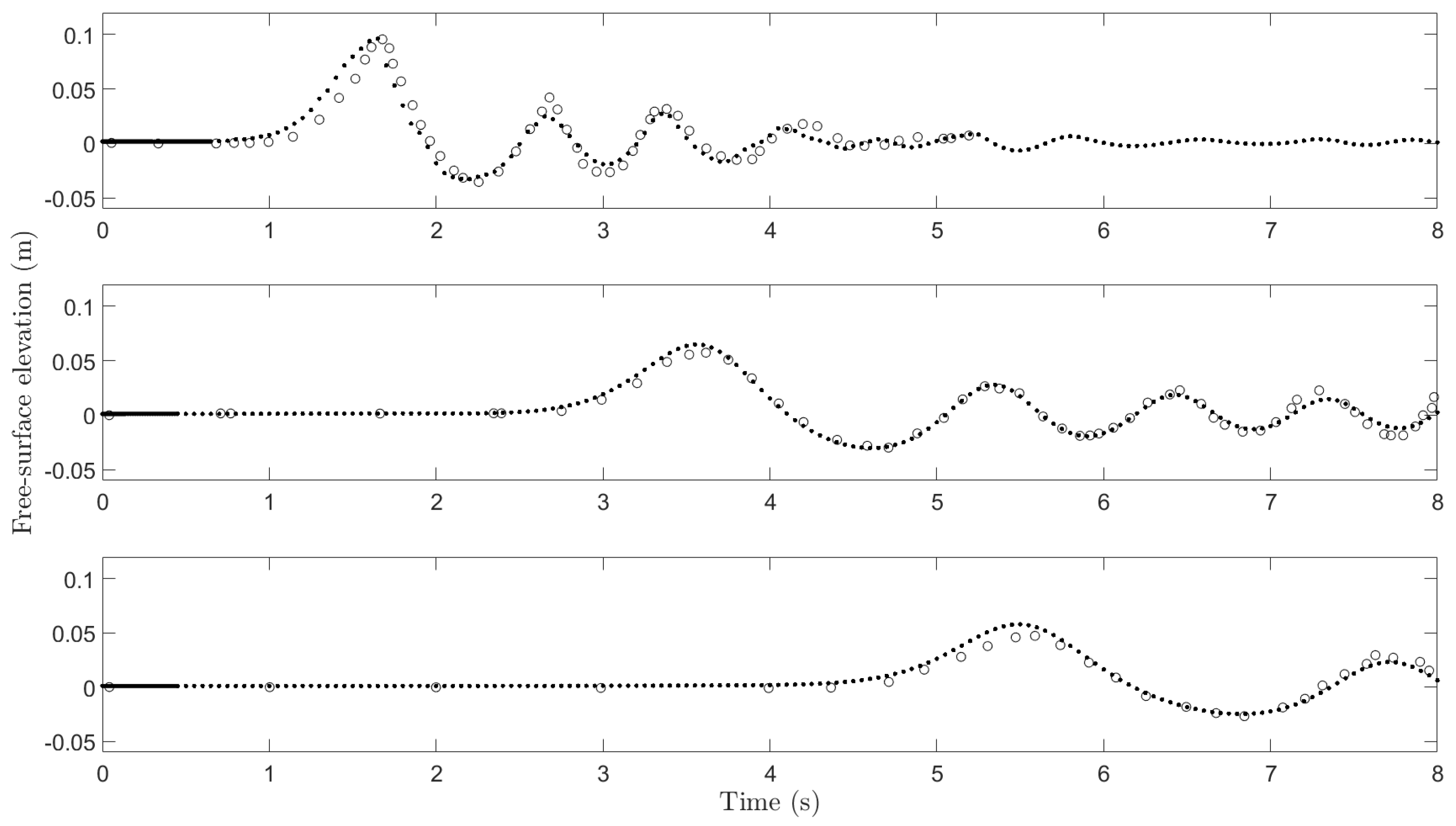
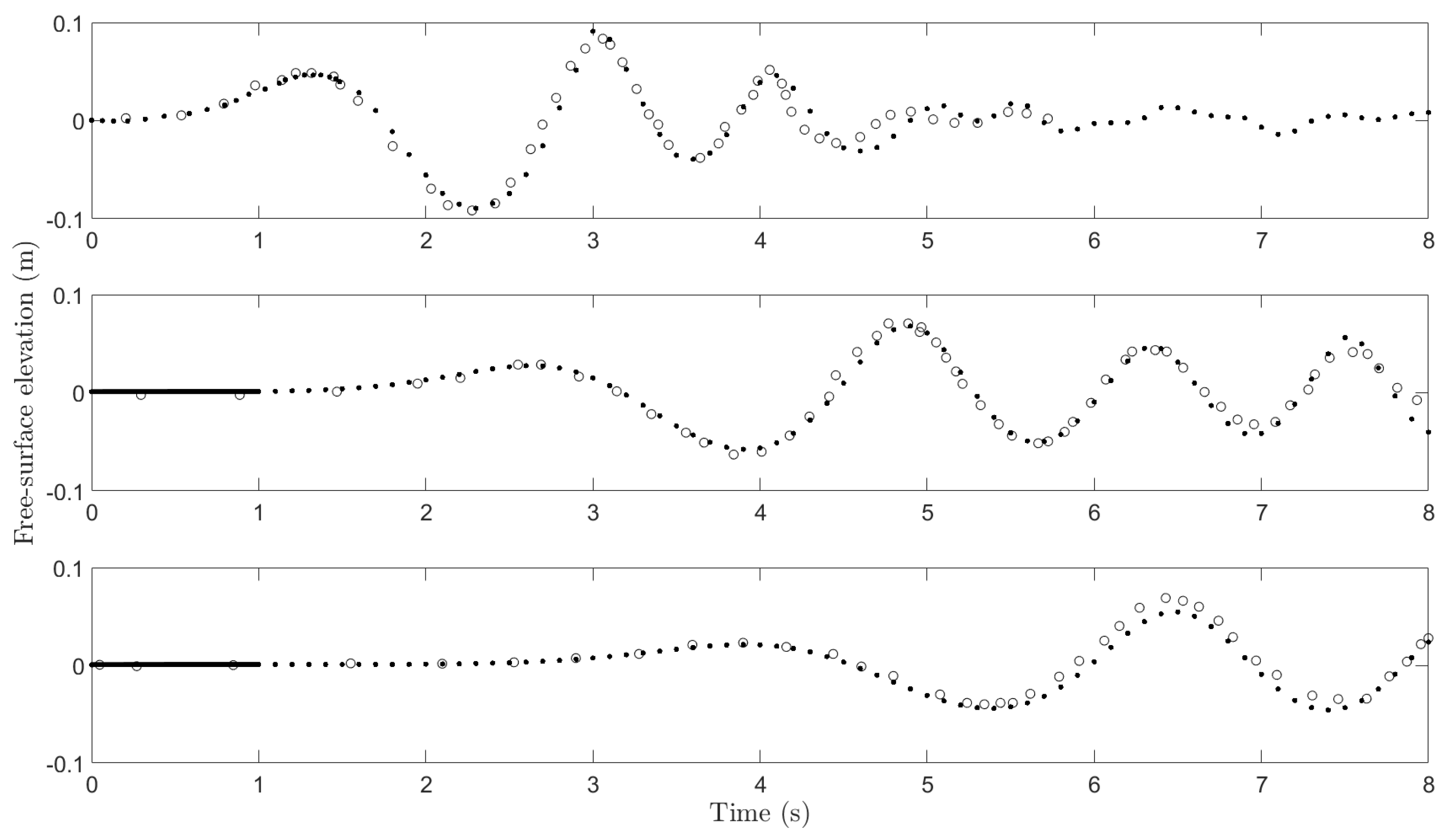
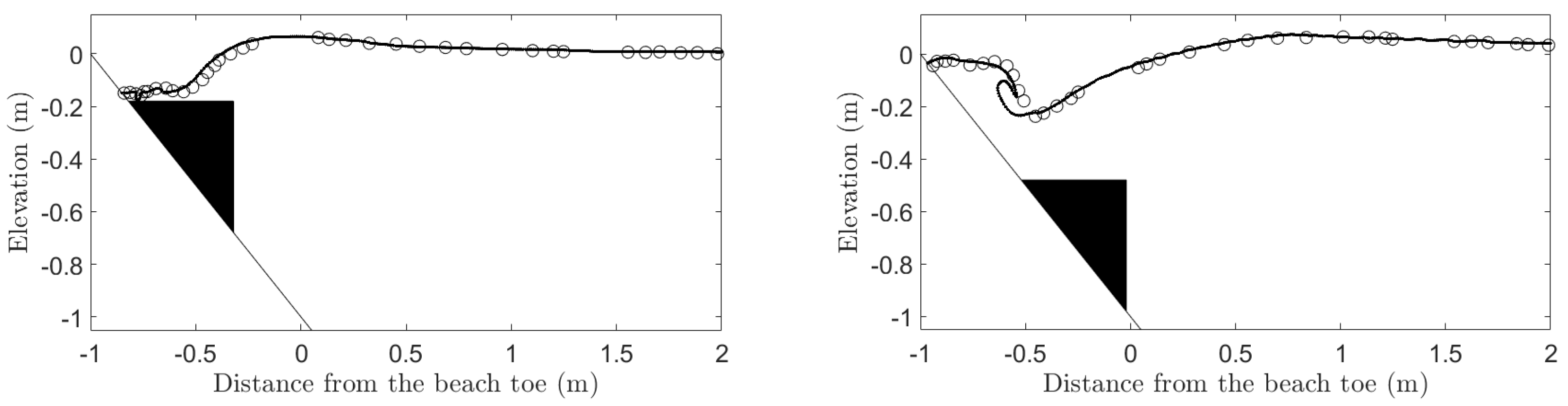
2.2. Model Validation

In order to examine the performance of the OpenFOAM-based numerical model for landslide impulsive waves and test the temporal and spatial resolution requirements, we use our model to numerically reproduce the relevant laboratory experiments reported by Heinrich [51]. The canonical geometry setup presented in Figure 1a was adopted in the experiment, with the wave tank having a specific configuration of 20 m in length, 0.55 m in width, and a constant depth of 0.4 m. Impulsive waves were generated by a subaerial solid box sliding freely down a 45 plane slope. The slide was in the shape of an isosceles right triangular prism with mass 105 kg, base sides 0.5 m, and length equal to the width of the tank. Initially, the entire solid box was just above the still free surface. Using a hydraulic jack system, the solid slide was released abruptly from rest and moved downhill by gravity. A 5 cm high rubber buffer was placed at the toe of the beach to stop the moving slide. Electrical contact-type wave gauges were employed to record wave heights at various locations. A 35 mm camera was also used to capture the free-surface profile at 32 frames per second.
In Figure 2, we compare the simulated free-surface profiles at three time instants, i.e., t = 0.6 , 1.0 , 1.5 s, with the laboratory data obtained by Heinrich [51]. Time histories of free-surface elevation at select locations ( x = 4 , 8 , 12 m) are also compared and presented in Figure 3. Visually, our simulations agree reasonably with the measurements as evidenced by the favorable comparisons shown in these figures. We remind the reader that characteristics of these impulsive waves have been discussed in detail by Heinrich [51], so we do not repeat them here.
Although the focus of the present study is on subaerial landslides, as a further check, we also reproduce Heinrich’s laboratory testing on waves generated by a submarine slide reported in the same study [51]. In this case, the fully submerged solid slide was initially set at rest with its top sitting 1 cm below the undisturbed free surface. The mass of the triangular prism-shaped solid slide was increased to 140 kg and the constant water depth was deeper at 1 m. Other experimental settings remained the same. The corresponding results are shown in Figure 4 and Figure 5, where we present the snapshots of free-surface profile at two different time instants and records of free-surface elevation at three fixed locations, respectively. Encouraging agreements are again observed across all comparisons.
Overall, the agreement between model predictions and laboratory measurements is satisfactory, suggesting that our OpenFOAM-based numerical model for landslide impulsive waves is quite capable. We remark that, as in most numerical modeling work, the above validation is achieved after a considerable amount of resolution tests and mesh refinement. Results presented here are obtained using a Courant number fixed at 0.4 and a spatial resolution of 0.5 cm.

3. Numerical Experiments

We shall now introduce a set of numerical experiments that can be used to help us examine more carefully how the slide shape affects the generation of impulsive waves by subaerial solid slides. These experiments are then realized by our computational model, which has been validated in Section 2.2. Results of important quantities such as wave amplitude, wave period, energy conversion, and the evolution of leading waves are presented and discussed.

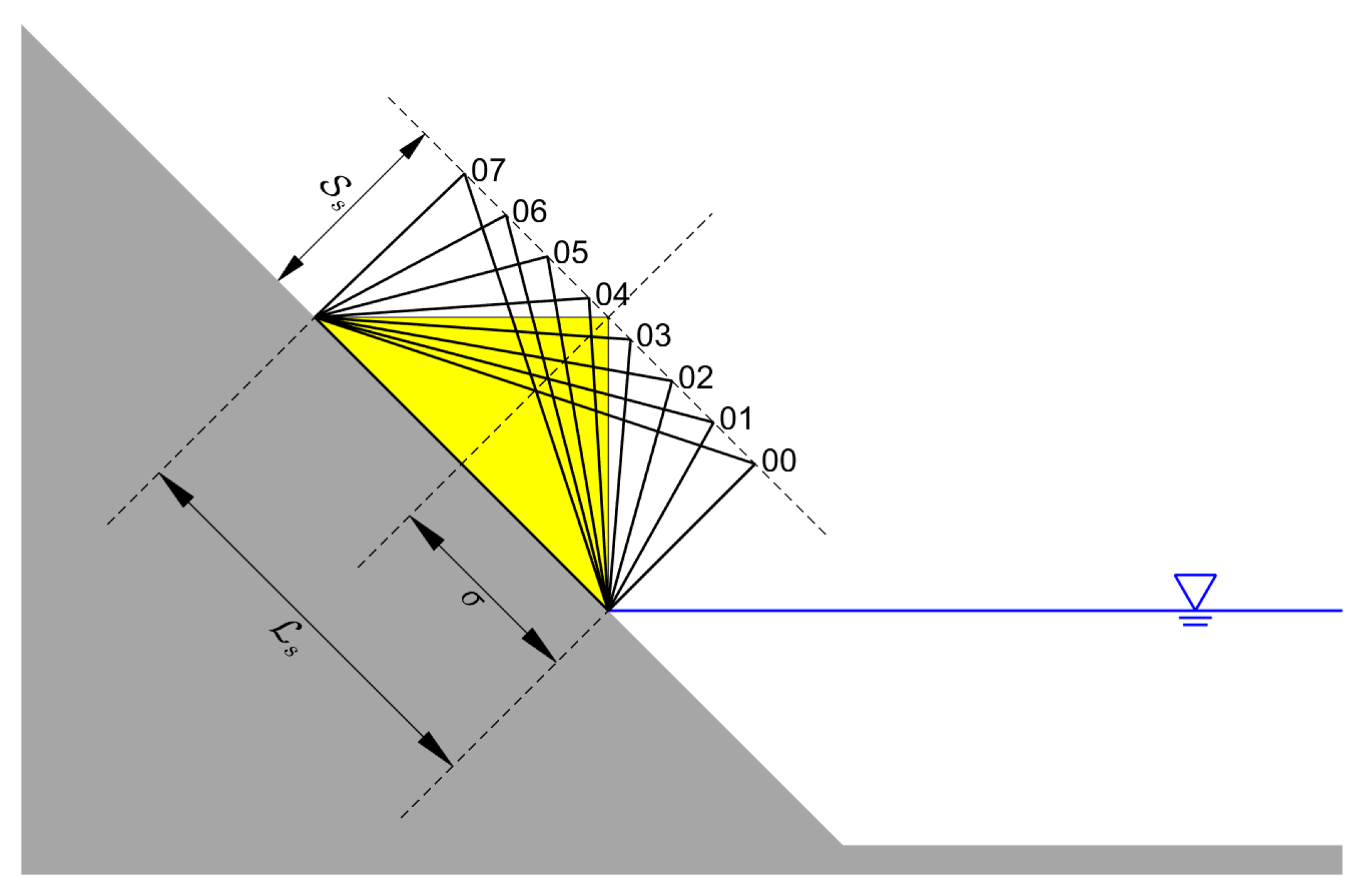
3.1. Design of Numerical Experiments

The main objective is to facilitate a more thorough understanding of particular significance of slide shape on landslide generated waves. As such, it would be convenient to use the laboratory testing by Heinrich [51] as the baseline problem and produce more relevant new cases for a systematic analysis. Specifically, in our simulations, we adopt the same experimental setup that has been used for model verification in Section 2.2, but use several sets of different solid slides for wave generation. In our simulations, we require these model slides to be triangular prisms with the same volume as the subaerial slide used by Heinrich [51], suggesting that they must have different triangular bases. The reason to limit ourselves to only triangular prisms is twofold. Firstly, we shall take advantage of the experimental data as ground truth, which is numerically beneficial, as this helps us avoid resolution problem and other possible numerical issues. Secondly, it would be more difficult to have a quantitative description of the slide shape parameter if solid slides in arbitrary three-dimensional shapes are used instead. Following this line of thought, by making reference to the solid slide used in the physical modeling and further requiring the model slides to have the same maximum slide thickness S s , as shown in Figure 6, we design 8 different prism-shaped slides of equal volume to be used in our numerical experiments. Since these model slides all have triangular bases, the characteristic of slide shape can be readily described by a single slide shape parameter σ defined in Figure 6, which indicates the relative position of the maximum slide thickness S s . In our setting, σ is related to slide front angle ϕ (see Figure 1a), representing the front face steepness of a solid slide, i.e., a slide with a larger value of σ (or ϕ ) has a steeper front face. Regarding the baseline solid slide from the laboratory testing, since its base is an isosceles right triangle with equal sides measuring 0.5 m, it has ϕ = 45 , σ 0.35 m, slide length L s 0.707 m, and S s 0.354 m. Accordingly, our model slides are designed to have σ ranging from 0 to 0.7 m with a uniform increment of 0.1 m. For convenience, these 8 model slides are labeled as Case 00 to Case 07, where the two-digit case number implies the value of σ . Table 1 tabulates values of σ and ϕ for these slides. Using the above design for numerical experiments, we shall be able to focus exclusively on the effects of slide shape, with minimal impact by the slide volume ( V S ), slide length ( L S ), maximum slide thickness ( S S ), and beach slope ( β ), which have been widely regraded as the most dominant factors controlling the wave generation by landslides [35,36,42,43,44,45].

3.2. Results and Discussions

Here, we present and discuss important properties of resulting impulsive waves observed in our numerical experiments, including maximum wave crest amplitude and its location, wave period, impact energy conversion, and evolution of free-surface profile, which have been commonly used in the literature to describe characteristics of landslide-generated waves [35,36,43].

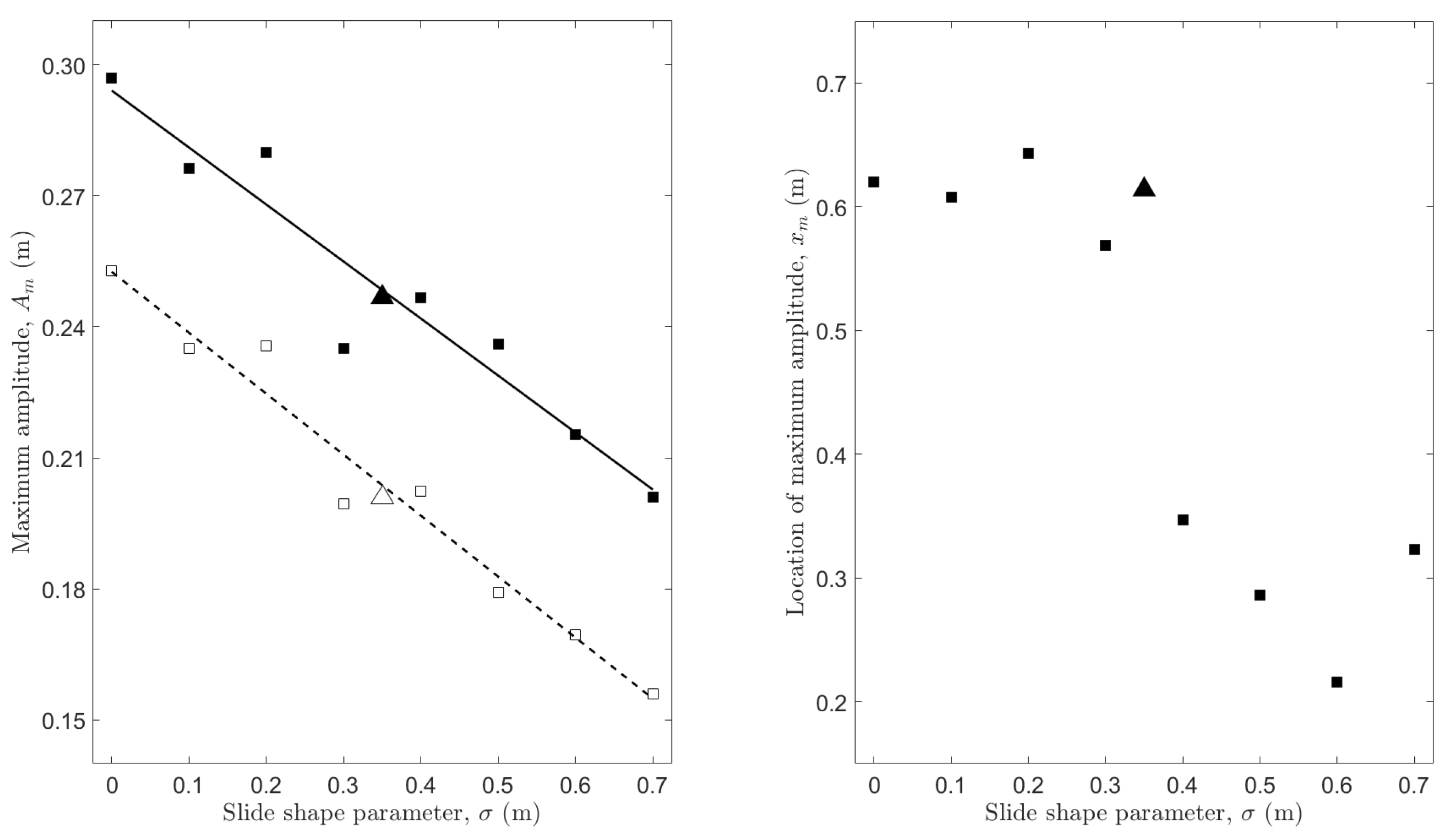
3.2.1. Maximum Amplitude and Its Location
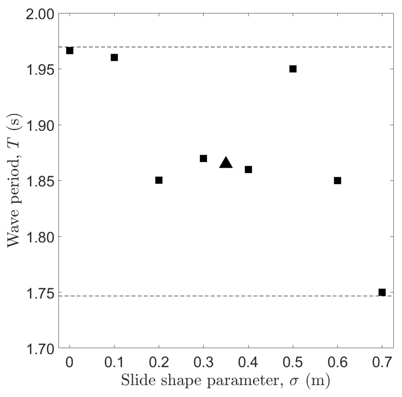
Wave amplitude is regarded as one of the most important wave characteristics for coastal hazard management, as it is often used to estimate maximum run-up height. Hence, in Figure 7, we first examine the effects of slide shape on maximum wave amplitude, A m , and its location along the streamwise direction, x m . We observe in our numerical experiments that A m is inversely proportional to slide shape parameter σ with a coefficient of determination R 2 0.92 , implying that a slide with a steeper front face generates a larger wave. We are of the view that this can be attributed to the fact that, for a model solid slide, the steeper the front face, the larger the effective contact surface when the smash of free surface commences abruptly, hence causing a greater impulsive impact. The impact of slide shape is considerable, as the difference in maximum amplitude can be as much as 50% if we compare Case 00 with another extreme run Case 07. The dependence of x m on σ , on the other hand, is not that clear since overall these ( x m , σ ) pairs seem to be scattered randomly in the plot. However, we notice from the results presented in Figure 7 that Case 00 to 03 have x m 0.6 m while x m is broadly around 0.3 m for Case 04 to 07. As a reference, we recall the slide length is fixed at L s = 0.707 m. Our observation suggests that x m can be categorized into two classes based on whether σ is less than 0.35 m, the corresponding slide shape parameter of the reference subaerial slide used in the physical modeling. Recall the symmetric shape of the reference slide and the sketch of model slides illustrated in Figure 6, Case 00 to 03 all have back (negative) skewed triangular bases while Case 04 to 07 are front (positive) skewed. It is also convenient to use the included angle θ defined in Figure 1a as the indicator since θ is an acute angle for Case 00 to 03 but an obtuse angle for Case 04 to 07.
In both physical and numerical experiments, maximum wave amplitude is commonly determined by comparing wave gauge records collected at a finite number of stations. Although we are more flexible to install a much denser array of numerical gauge stations, searching for the location of the maximum amplitude, x m , remains challenging. Therefore, we shall examine the effects of slide shape on wave amplitude at a fixed location. In this regard, in Figure 7 we also plot wave amplitude as a function of σ at x = 1 m. We recall that x m ranges roughly between 0.3 and 0.6 m, as has been discussed previously. We note that x = 1 m, which is in the constant depth region, is far enough from all x m , but is not too far away such that frequency dispersion is not dominant over the wave amplitude. As can be seen from Figure 7, local wave amplitude is also inversely proportional to σ with R 2 0.96 . We also witness the decay of maximum amplitude to the local amplitude at this station, which is reasonable as waves propagate further downhill into a deeper water. Overall, the amplitude decay is roughly around 20% across all cases.

3.2.2. Wave Period

Figure 8 shows the wave period, T, determined by the gauge records at x = 1 m for all cases. Our results suggest that wave period is independent of slide shape parameter σ . In fact, T is within a ± 6 % range across all cases. This is in agreement of the laboratory findings reported in the literature, where wave period is mainly controlled by the slide volume and the slide Froude number defined as [35].
Fr s = v s g h ,
where v s = slide impact velocity, g = gravitational acceleration, and h = water depth.

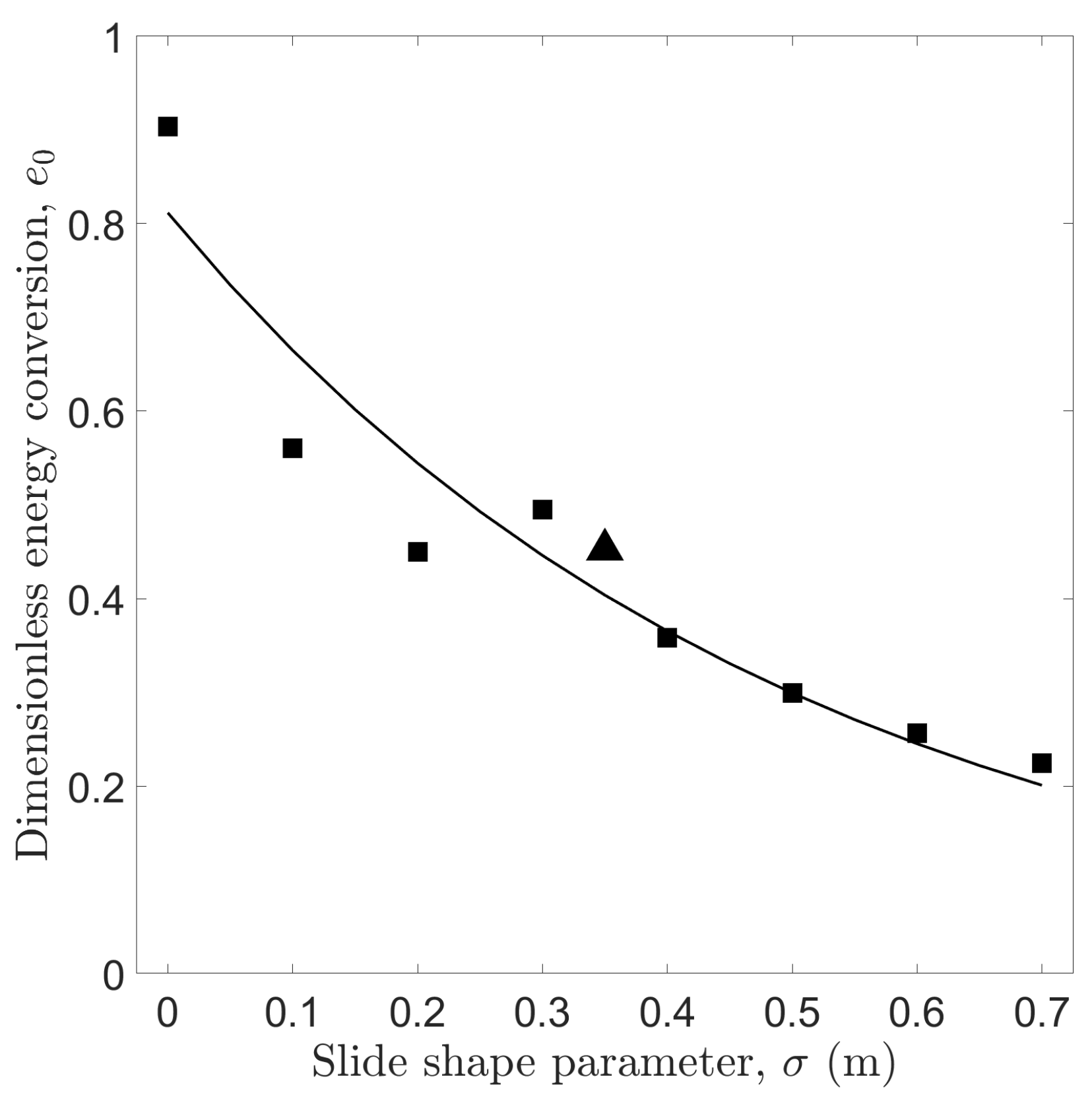
3.2.3. Impact Energy Conversion

The energy conversion efficiency from solid slide energy into water wave energy is often evaluated by the ratio of impulsive wave energy, E w ( 0 ) , to the maximum kinetic slide impact energy, E s , defined as [36]
e 0 = E w ( 0 ) E s = ρ g c η 2 d t ρ s v s 2 A s ,
where ρ = water density, c = wave celerity, η = free-surface displacement, ρ s = density of slide, and A s = solid block volume per unit width. Previous laboratory studies [35,43] have suggested that the energy conversion ratio, e 0 , depends on slide Froude number Fr s , slide volume V s , and maximum slide thickness S s . Here, we exclusively examine the effects of slide shape on the energy conversion efficiency by plotting e 0 under various values of σ , as presented in Figure 9. Our results reflect a clear dependency of e 0 on the slide shape parameter, σ . In fact, a curve fitting using the exponential model e 0 = c 1 exp ( c 2 σ ) yields a reasonable result with R 2 = 0.93 . We observe that a slide with a steeper front face (small σ and θ , large ϕ ) is more efficient in generating impulsive waves. Consequently, the resulting maximum wave amplitude is larger, as has been discussed in Section 3.2.1. Except the extreme Case 00 that has a vertical front face and hence an exceptional large e 0 as can be expected, in our experiments, e 0 lies below 0.6, which is in agreement with the laboratory results reported in literature [35,43].

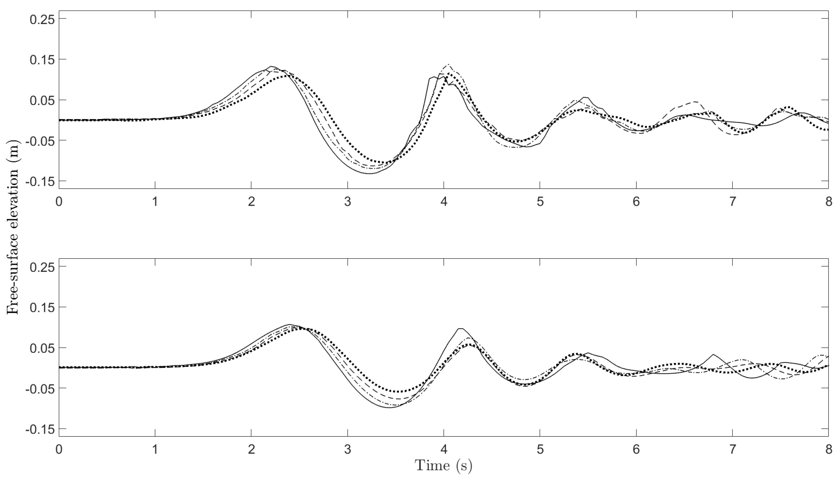
3.2.4. Evolution of Leading Waves

Leading tsunami waves are often used as the model wave for the prediction of the arrival time and maximum runup height of tsunami waves [41]. The leading wave group often consists of a few successive waves and the first wave crest may not always be the largest [35]. To provide a clear picture of the evolution of leading waves, Figure 10 shows the records of free-surface elevation at four stations in the constant depth region located at x = 1 , 3 , 5 , 7 m for both Case 00 and Case 07, two representative slides that have the steepest and mildest front faces, respectively. Let us first focus on the evolution of leading waves for Case 00. We observe from Figure 10 that the leading wave group of Case 00 evolves considerably from x = 1 m to x = 5 m, but the wave profile remains more or less the same afterwards. Although the first wave crest is significantly larger than the second one at x = 1 m, the second crest takes over at x = 3 m and remains the largest. Figure 10 also reveals that from x = 3 m to x = 7 m, the first wave crest travels at the typical long wave speed, c = c 0 = g h 0 , while a smaller phase speed, c 0.89 c 0 , is observed between x = 1 m and x = 3 m. For the second crest, c 0.84 c 0 between x = 1 m to x = 3 m, but the phase speed decreases to a constant value at c 0.79 c 0 for x > 3 m. The observed phase speeds of both the first and the second crests agree with the general trend of the laboratory data reported in literature [35].
For Case 07, we see clearly from Figure 10 that the evolution of leading group is only noticeable from x = 1 m to x = 3 m. Furthermore, the first crest is always larger than the second one. The phase speed of the first peak is about 0.89 c 0 between x = 1 m and x = 3 m and c c 0 for x > 3 m, which is the same as that of Case 00. For the second peak, c 0.65 c 0 between x = 1 m and x = 3 m, c 0.68 c 0 from x = 3 m to x = 5 m, and c 0.75 c 0 between the last two stations. This is slightly different from what we have observed for Case 00.
Figure 10 also reveals that, compared to the results of Case 07, Case 00 always has larger local maximum amplitudes at these four numerical gauge stations. However, the difference becomes insignificant at x = 7 m. This implies that the slide shape parameter σ has only secondary effects on wave amplitude when waves propagate sufficiently far from the initial impact region, while σ controls the global maximum amplitude A m , occurring at x = x m 0.3 , 0.6 m as has been previously discussed in Section 3.2.1.
In short, the results from two representative cases shown in Figure 10 suggest that the effects of slide shape parameter σ can be important in the region close to the sloping beach, the so-called generation region where impulsive waves are being generated by the solid slide. To further provide more direct evidence, in Figure 11 and Figure 12 we present the records of surface profile for all cases at x = 1 m and x = 7 m, respectively. We note that x = 1 m can be loosely referred as the near field while the x = 7 m is seen as the far field. In the near field region, Figure 11 reveals the slide shape parameter σ indeed plays a considerable role as the differences in wave shapes can be clearly observed across cases with different slide shapes. However, Figure 12 shows that, with only minor modulation, the resulting wave profiles can be categorized into two groups, one consists of Case 00 to Case 03, the other includes Case 04 to Case 07. For each group, all leading waves collapse into a single profile in the far field, reflecting the fact that the frequency dispersion dominates while the slide shape parameter becomes irrelevant.
Recall from Figure 10 that for Case 00 the second crest is larger than the first in the far field while the first crest is always the largest at all stations for Case 07. To gain a better idea on which crest is potentially more threatening, in Figure 13 we compare the amplitude of the first crest ( A m , 1 ) with that of the second crest ( A m , 2 ) recorded at x = 7 m for all cases examined in our numerical experiments. To make a concise presentation, the amplitude ratio, A m , 1 to A m , 2 , is plotted in the figure. It is intriguing to see that for Case 00 to Case 03 (back skewed), in the far field, the second crest is always larger than the first crest while the opposite is observed for Case 04 to Case 07 (front skewed). In other words, the amplitude ratio depends linearly on σ with R 2 0.92 . In all, this again reflects that the shape skewness, hence the slide shape indeed can have a significant impact on impulsive waves generated by a subaerial solid slide.

4. Concluding Remarks

Destructive tsunamis can be triggered by massive landslides and pose significant threats to human life, critical infrastructure, economies, and environments in many coastal communities. To facilitate a better understanding of the physical mechanism of impulsive waves generated by a subaerial solid slide, the particular effects of slide shape on the characteristics of impulsive waves are investigated through a set of carefully designed numerical experiments realized by a new OpenFOAM-based computational model for landslide impulsive waves. Specifically, we examine how the shape of solid slide affects the maximum wave amplitude, wave period, slide energy conversion ratio, and the evolution of leading waves. We believe that our analysis generates some encouraging and useful results. Based on the observations from the numerical experiments, the following main findings are reported:
  • Maximum wave amplitude, A m , is inversely proportional to the slide shape parameter, σ . Location of the maximum amplitude, x m , also depends on σ (Section 3.2.1).
  • Wave period, T, is almost independent of σ (Section 3.2.2).
  • Impact energy conversion ratio, e 0 , decays exponential with σ (Section 3.2.3).
  • The first crest always travels at the typical long wave speed while the second crest propagates at a speed about 15 to 25% slower depending on the value of σ (Section 3.2.4).
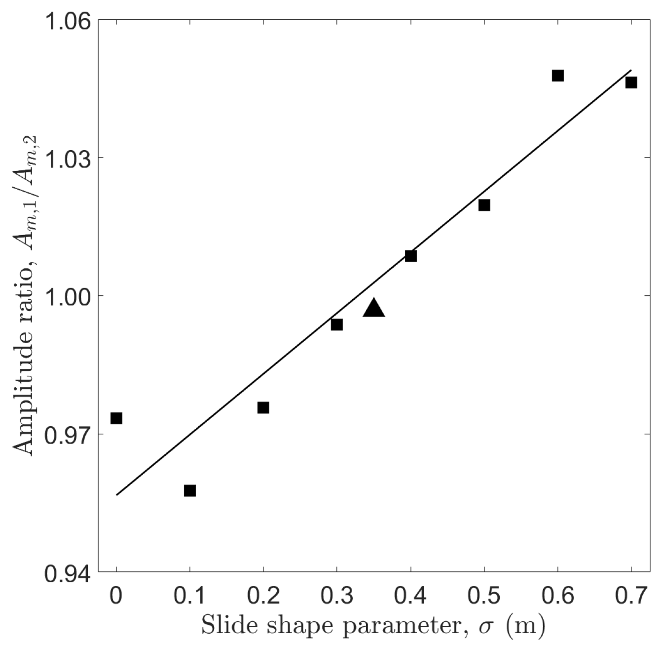
  • In the far field, the second crest becomes larger than the first crest if σ is smaller (Section 3.2.4).
Overall, the present numerical experiments reveal that the slide shape can have dominant effects on the characteristics of impulsive waves generated by a subaerial solid slide. We remark that our experiments are specially designed so that the slide shape becomes the only factor. Furthermore, only simple solid slides, whose slide shape can be described by single parameter σ , are considered. Extreme cases, such as a slide with a vertical front face ( σ = 0 ), are also examined in our experiments. Of course, in reality these conditions may never be met. For instant, slide properties like slide volume, slide length, maximum slide thickness, etc., are all related to each other and must be considered as a whole. It is also nearly impossible to have a slide mass with a vertical front face. Having said that, we believe our findings, although based on a set of idealized and well controlled experiments, are valuable. Theoretically speaking, we identify how and when the effects of slide shape on landslide generated impulsive waves become significant. We believe this aspect is important in order to facilitate a more thorough undemanding of the complex wave generation mechanism in landslide tsunamis.

Author Contributions

C.-S.H. designed and performed the numerical experiments. I.-C.C. prepared the manuscript. All authors have read and agreed to the published version of the manuscript.

Funding

This research was funded by the National Science and Technology Council, Taiwan [108-2221-E-002-057-MY2; 111-2221-E-002-110].

Acknowledgments

We thank the anonymous reviewers for their careful reading of the manuscript. Their constructive feedback has helped improve and clarify our paper.

Conflicts of Interest

The authors declare no conflict of interest.

References

  1. Slingerland, R.L.; Voight, B. Occurrences, properties and predictive models of landslide-generated impulse waves. In Rockslides and Avalanches; Voight, B., Ed.; Elsevier: Amsterdam, The Netherlands, 1979; Volume 2, pp. 317–397. [Google Scholar]
  2. Ward, S.N. Landslide tsunami. J. Geophys. Res. Solid Earth 2001, 106, 11201–11215. [Google Scholar] [CrossRef]
  3. Fritz, H.M.; Hager, W.H.; Minor, H.-E. Lituya Bay case: Rockslide impact and wave run-up. Sci. Tsunami Hazards 2001, 19, 3–22. [Google Scholar]
  4. Bardet, J.-P.; Synolakis, C.E.; Davies, H.L.; Imamura, F.; Okal, E.A. Landslide tsunamis: Recent findings and research directions. Pure Appl. Geophys. 2003, 160, 1793–1809. [Google Scholar] [CrossRef]
  5. Fritz, H.M.; Mohammed, F.; Yoo, J. Lituya Bay landslide impact generated mega-tsunami 50th anniversary. Pure Appl. Geophys. 2009, 166, 153–175. [Google Scholar] [CrossRef]
  6. Miller, D.J. Giant Waves in Lituya Bay, Alaska; Geological Survey Professional Paper 354-C; U.S. Government Printing Office: Washington, DC, USA, 1960.
  7. Higman, B.; Shugar, D.H.; Stark, C.P.; Ekström, G.; Koppes, M.N.; Lynett, P.; Dufresne, A.; Haeussler, P.J.; Geertsema, M.; Gulick, S.; et al. The 2015 landslide and tsunami in Taan Fiord, Alaska. Sci. Rep. 2018, 8, 12993. [Google Scholar] [CrossRef]
  8. Haeussler, P.J.; Gulick, S.P.S.; McCall, N.; Walton, M.; Reece, R.; Larsen, C.; Shugar, D.H.; Geertsema, M.; Venditti, J.G.; Labay, K. Submarine deposition of asubaerial landslide in Taan Fiord, Alaska. J. Geophys. Res. Earth Surf. 2018, 123, 2443–2463. [Google Scholar] [CrossRef]
  9. Ward, S.N.; Day, S. The 1958 Lituya Bay Landslide and Tsunami—A tsunami ball approach. J. Earthq. Tsunami 2010, 4, 285–319. [Google Scholar] [CrossRef]
  10. Franz, M.; Jaboyedoff, M.; Mulligan, R.P.; Podladchikov, Y.; Take, W.A. An efficient two-layer landslide-tsunami numerical model: Effects of momentum transfer validated with physical experiments of waves generated by granular landslides. Nat. Hazards Earth Syst. Sci. 2021, 21, 1229–1245. [Google Scholar] [CrossRef]
  11. L’Heureux, J.-S.; Hansen, L.; Longva, O.; Eilertsen, R.S. Landslides Along Norwegian Fjords: Causes and Hazard Assessment. In Landslide Science and Practice; Margottini, C., Canuti, P., Sassa, K., Eds.; Springer: Berlin/Heidelberg, Germany, 2013; Volume 5, pp. 317–397. [Google Scholar]
  12. Glimsdal, S.; L’Heureux, J.-S.; Harbitz, C.B.; Løvholt, F. The 29th January 2014 submarine landslide at Statland, Norway—Landslide dynamics, tsunami generation, and run-up. Landslides 2016, 13, 1435–1444. [Google Scholar] [CrossRef]
  13. Harbitz, C.B.; Pedersen, G.; Gjevik, B. Numerical simulations of large water waves due to landslides. J. Hydraul. Eng. 1993, 119, 1325–1342. [Google Scholar] [CrossRef]
  14. Harbitz, C.B.; Glimsdal, S.; Løvholt, F.; Kveldsvik, V.; Pedersen, G.K.; Jensen, A. Rockslide tsunamis in complex fjords: From an unstable rock slope at Åkerneset to tsunami risk in western Norway. Coast. Eng. 2014, 88, 101–122. [Google Scholar] [CrossRef]
  15. Dahl-Jensen, T.; Larsen, L.M.; Pedersen, S.A.S.; Pedersen, J.; Jepsen, H.F.; Pedersen, G.; Nielsen, T.; Pedersen, A.K.; Von Platen-Hallermund, F.; Weng, W. Landslide and Tsunami 21 November 2000 in Paatuut, West Greenland. Nat. Hazards 2004, 31, 277–287. [Google Scholar] [CrossRef]
  16. Gauthier, D.; Anderson, S.A.; Fritz, H.M.; Giachetti, T. Karrat Fjord (Greenland) tsunamigenic landslide of 17 June 2017: Initial 3D observations. Landslides 2018, 15, 327–332. [Google Scholar] [CrossRef]
  17. Couston, L.-A.; Mei, C.C.; Alam, M.-R. Landslide tsunamis in lakes. J. Fluid Mech. 2015, 772, 784–804. [Google Scholar] [CrossRef]
  18. Barla, G.; Paronuzzi, P. The 1963 Vajont Landslide: 50th Anniversary. Rock Mech. Rock Eng. 2013, 46, 1267–1270. [Google Scholar] [CrossRef]
  19. Waldmann, N.; Vasskog, K.; Simpson, G.; Chapron, E.; Støren, E.W.N.; Hansen, L.; Loizeau, J.-L.; Nesje, A.; Ariztegui, D. Anatomy of a catastrophe: Reconstructing the 1936 rock fall and tsunami event in Lake Lovatnet, Western Norway. Front. Earth Sci. 2021, 9, 671378. [Google Scholar] [CrossRef]
  20. Plafker, G.; Eyzaguirre, V.R. Rock Avalanche and Wave at Chungar, Peru. In Developments in Geotechnical Engineering; Voight, B., Ed.; Elsevier: Amsterdam, The Netherlands, 1979; Volume 14, pp. 269–279. [Google Scholar]
  21. Panizzo, A.; De Girolamo, P.; Di Risio, M.; Maistri, A.; Petaccia, A. Great landslide events in Italian artificial reservoirs. Nat. Hazards Earth Syst. Sci. 2005, 5, 733–740. [Google Scholar] [CrossRef]
  22. Kilburn, C.R.J.; Petley, D.N. Forecasting giant, catastrophic slope collapse: Lessons from Vajont, Northern Italy. Geomorphology 2003, 54, 21–32. [Google Scholar] [CrossRef]
  23. Paronuzzi, P.; Bolla, A. The prehistoric Vajont rockslide: An updated geological model. Geomorphology 2012, 169, 165–191. [Google Scholar] [CrossRef]
  24. Delatte, N.J. Beyond Failure, Forensic Case Studies for Civil Engineers; ASCE Press: Reston, VA, USA, 2009; pp. 234–248. [Google Scholar]
  25. Lynett, P.J.; Borrero, J.C.; Liu, P.L.-F.; Synolakis, C.E. Field survey and numerical simulations: A review of the 1998 Papua New Guinea Tsunami. Pure Appl. Geophys. 2003, 160, 2119–2146. [Google Scholar] [CrossRef]
  26. Liu, P.L.-F.; Higuera, P.; Husrin, S.; Prasetya, G.S.; Prihantono, J.; Diastomo, H.; Pryambodo, D.G.; Susmoro, H. Coastal landslides in Palu Bay during 2018 Sulawesi earthquake and tsunami. Landslides 2020, 17, 2085–2098. [Google Scholar] [CrossRef]
  27. Grilli, S.T.; Tappin, D.R.; Carey, S.; Watt, S.F.L.; Ward, S.N.; Grilli, A.R.; Engwell, S.L.; Zhang, C.; Kirby, J.T.; Schambach, L.; et al. Modelling of the tsunami from the December 22, 2018 lateral collapse of Anak Krakatau volcano in the Sunda Straits, Indonesia. Sci. Rep. 2019, 9, 11946. [Google Scholar] [CrossRef] [PubMed]
  28. Masson, D.G.; Harbitz, C.B.; Wynn, R.B.; Pedersen, G.; Løvholt, F. Submarine landslides: Processes, triggers and hazard prediction. Phil. Trans. R. Soc. A 2006, 364, 2009–2039. [Google Scholar] [CrossRef] [PubMed]
  29. Harbitz, C.B.; Løvholt, F.; Bungum, H. Submarine landslide tsunamis: How extreme and how likely? Nat. Hazards 2014, 72, 1341–1374. [Google Scholar] [CrossRef]
  30. Parsons, T.; Geist, E.L.; Ryan, H.F.; Lee, H.J.; Haeussler, P.J.; Lynett, P.; Hart, P.E.; Sliter, R.; Rol, E. Source and progression of a submarine landslide and tsunami: The 1964 Great Alaska earthquake at Valdez. J. Geophys. Res. Solid Earth 2014, 119, 8502–8516. [Google Scholar] [CrossRef]
  31. Okal, E. Normal mode energetics for far-field tsunamis generated by dislocations and landslides. Pure Appl. Geophys. 2003, 160, 2189–2221. [Google Scholar] [CrossRef]
  32. Ruff, L.J. Some aspects of energy balance and tsunami generation by earthquakes and landslides. Pure Appl. Geophys. 2003, 160, 2155–2167. [Google Scholar] [CrossRef]
  33. Synolakis, C.E.; Bardet, J.-P.; Borrero, J.C.; Davies, H.L.; Okal, E.A.; Silver, E.A.; Sweet, S.; Tappin, D.R. The slump origin of the 1998 Papua New Guinea Tsunami. Proc. R. Soc. Lond. A 2002, 458, 763–789. [Google Scholar] [CrossRef]
  34. Liu, P.L.-F.; Wu, T.-R.; Raichlen, F.; Synolakis, C.E.; Borrero, J.C. Runup and rundown generated by three-dimensional sliding masses. J. Fluid Mech. 2005, 536, 107–144. [Google Scholar] [CrossRef]
  35. Fritz, H.M.; Hager, W.H.; Minor, H.-E. Near field characteristics of landslide generated impulse waves. J. Waterw. Port Coast. Ocean Eng. 2004, 130, 287–302. [Google Scholar] [CrossRef]
  36. Watts, P. Tsunami features of solid block underwater landslides. J. Waterw. Port Coast. Ocean Eng. 2000, 126, 144–152. [Google Scholar] [CrossRef]
  37. Liu, P.L.-F.; Lynett, P.; Synolakis, C.E. Analytical solutions for forced long waves on a sloping beach. J. Fluid Mech. 2003, 478, 101–109. [Google Scholar] [CrossRef]
  38. Wang, Y.; Liu, P.L.-F.; Mei, C.C. Solid landslide generated waves. J. Fluid Mech. 2011, 675, 529–539. [Google Scholar] [CrossRef]
  39. Lee, C.-H.; Huang, Z. Multi-phase flow simulation of impulsive waves generated by a sub-aerial granular landslide on an erodible slope. Landslides 2020, 18, 881–895. [Google Scholar] [CrossRef]
  40. Synolakis, C.E. Tsunamis and seiches. In Earthquake Engineering Handbook; Chen, W.-F., Scawthorn, C., Eds.; CRC Press: Boca, FL, USA, 2003; pp. 1–90. [Google Scholar]
  41. Synolakis, C.E. The runup of solitary waves. J. Fluid Mech. 1987, 185, 523–545. [Google Scholar] [CrossRef]
  42. Walder, J.S.; Watts, P.; Sorensen, O.E.; Janssen, K. Water waves generated by subaerial mass flows. J. Geophys. Res. Solid Earth 2003, 108, 226–2255. [Google Scholar]
  43. Ataie-Ashtiani, B.; Nik-Khah, A. Impulsive waves caused by subaerial landslides. Environ. Fluid Mech. 2008, 8, 263–280. [Google Scholar] [CrossRef]
  44. Watts, P.; Grilli, S.T.; Tappin, D.R.; Fryer, G.J. Tsunami generation by submarine mass failure. II: Predictive equations and case studies. J. Waterw. Port Coast. Ocean Eng. 2005, 131, 298–310. [Google Scholar] [CrossRef]
  45. Ataie-Ashtiani, B.; Najafi-Jilani, A. Laboratory investigations on impulsive waves caused by underwater landslide. Coast. Eng. 2008, 55, 989–1004. [Google Scholar] [CrossRef]
  46. Madsen, P.A.; Schäffer, H.A. Analytical solutions for tsunami runup on a plane beach: Single waves, N-waves and transient waves. J. Fluid Mech. 2010, 645, 25–57. [Google Scholar] [CrossRef]
  47. Barranco, I.; Liu, P.L.-F. Run-up and inundation generated by non-decaying dam-break bores on a planar beach. J. Fluid Mech. 2021, 915, 1–29. [Google Scholar] [CrossRef]
  48. Zweifel, A.; Hager, W.H.; Minor, H.-E. Plane impulse waves in reservoirs. J. Waterw. Port Coast. Ocean Eng. 2006, 132, 358–368. [Google Scholar] [CrossRef]
  49. Heller, V.; Hager, W.H. Wave types of landslide generated impulse waves. Ocean Eng. 2011, 38, 630–640. [Google Scholar] [CrossRef]
  50. Madsen, P.A.; Fuhrman, D.R.; Schäffer, H.A. On the solitary wave paradigm for tsunamis. J. Geophys. Res. 2008, 113, C12012. [Google Scholar] [CrossRef]
  51. Heinrich, P. Nonlinear water waves generated by submarine and aerial landslides. J. Waterw. Port Coast. Ocean Eng. 1992, 118, 249–266. [Google Scholar] [CrossRef]
  52. Fine, I.V.; Rabinovich, A.B.; Thomson, R.E.; Kulikov, E.A. Numerical modeling of tsunami generation by submarine and subaerial landslides. In Submarine Landslides and Tsunamis; Yalçiner, A.C., Pelinovsky, E.N., Okal, E., Synolakis, C.E., Eds.; Springer: Dordrecht, The Netherlands, 2003; Volume 21, pp. 69–88. [Google Scholar]
  53. LeBlond, P.H.; Jones, A.T. Underwater landslides ineffective at tsunami generation. J. Waterw. Port Coast. Ocean Eng. 1995, 13, 25–26. [Google Scholar]
  54. Weller, H.G.; Tabor, G.; Jasak, H.; Fureby, C. A tensorial approach to computational continuum mechanics using object-oriented techniques. Comput. Phys. 1998, 12, 620–631. [Google Scholar] [CrossRef]
  55. Higuera, P.; Lara, J.L.; Losada, I.J. Three–dimensional interaction of waves and porous coastal structures using OpenFOAM. Part II: Application. Coast. Eng. 2014, 83, 243–258. [Google Scholar] [CrossRef]
  56. Higuera, P.; Lara, J.L.; Losada, I.J. Simulating coastal engineering processes with OpenFOAM. Coast. Eng. 2013, 71, 119–134. [Google Scholar] [CrossRef]
  57. Higuera, P.; Losada, I.J.; Lara, J.L. Three-dimensional numerical wave generation with moving boundaries. Coast. Eng. 2015, 101, 35–47. [Google Scholar] [CrossRef]
  58. Higuera, P.; Liu, P.L.-F.; Lin, C.; Wong, W.-Y.; Kao, M.-J. Laboratory-scale swash flows generated by a non-breaking solitary wave on a steep slope. J. Fluid Mech. 2018, 847, 186–227. [Google Scholar] [CrossRef]
  59. Maza, M.; Lara, J.L.; Losada, I.J. Tsunami wave interaction with mangrove forests: A 3-D numerical approach. Coast. Eng. 2015, 98, 33–54. [Google Scholar] [CrossRef]
  60. Hirt, C.W.; Nichols, B.D. Volume of fluid (VOF) method for the dynamics of free boundaries. J. Comput. Phys. 1981, 39, 201–225. [Google Scholar] [CrossRef]
  61. Harlow, F.H.; Welch, J.E. Numerical calculation of time-dependent viscous incompressible flow of fluid with a free surface. Phys. Fluids 1965, 8, 2182–2189. [Google Scholar] [CrossRef]
  62. Osher, S.; Sethian, J.A. Fronts propagating with curvature-dependent speed: Algorithms based on Hamilton–Jacobi formulations. J. Comput. Phys. 1988, 79, 12–49. [Google Scholar] [CrossRef]
  63. Gingold, R.A.; Monaghan, J.J. Smoothed particle hydrodynamics: Theory and application to non-spherical stars. Mon. Not. R. Astron. Soc. 1977, 181, 375–389. [Google Scholar] [CrossRef]
  64. Cundall, P.A.; Strack, O.D.L. A discrete numerical model for granular assemblies. Géotechnique 1979, 29, 45–65. [Google Scholar] [CrossRef]
  65. Frisch, U.; Hasslacher, B.; Pomeau, Y. Lattice-gas automata for the Navier-Stokes equations. Phys. Rev. Lett. 1986, 56, 1505–1508. [Google Scholar] [CrossRef]
  66. Peskin, C.S. Flow patterns around heart valves: A numerical method. J. Comput. Phys. 1972, 10, 252–271. [Google Scholar] [CrossRef]
  67. Windt, C.; Davidson, J.; Chandar, D.D.J.; Faedo, N.; Ringwood, J.V. Evaluation of the overset grid method for control studies of wave energy converters in OpenFOAM numerical wave tanks. J. Ocean Eng. Mar. Energy 2020, 6, 55–70. [Google Scholar] [CrossRef]
  68. Heller, V.; Hager, W.H. Impulse product parameter in landslide generated impulse waves. J. Waterw. Port Coast. Ocean Eng. 2010, 136, 145–155. [Google Scholar] [CrossRef]
Figure 1. (a) Schematic (not drawn to scale) of the numerical wave tank: a solid slide moving downhill on a sloping beach connected to a region of constant depth h 0 . β is the beach slope, ϕ denotes the slide front angle [68], and θ shows the included angle formed by the slide front face and the still free surface. Origin of the coordinate system is set at the initial shoreline. (b) The computational domain and a sample numerical mesh. No-slip condition is required on all boundaries, except at the top boundary open to free atmosphere.
Water 14 02643 g001
Figure 2. Model validation for subaerial landslide generated waves: snapshots of free-surface profile at select time instants (Top to bottom: t = 0.6 , 1.0 , 1.5 s). Dot: model predictions. Circle: measurements reported by Heinrich [51].
Water 14 02643 g002
Figure 3. Model validation for subaerial landslide generated waves: records of free-surface elevation at fixed locations (Top to bottom: x = 4 , 8 , 12 m). Dot: model predictions. Circle: measurements reported by Heinrich [51].
Water 14 02643 g003
Figure 4. Reproduction of submarine landslide generated waves: snapshots of the free surface profile at two different time instants (Left: t = 0.5 s; Right: t = 1.0 s). Dot: model predictions. Circle: measurements reported by Heinrich [51].
Water 14 02643 g004
Figure 5. Reproduction of submarine landslide generated waves: records of free surface elevation at fixed locations (Top to bottom: x = 4 , 8 , 12 m). Dot: model predictions. Circle: measurements reported by Heinrich [51].
Water 14 02643 g005
Figure 6. Sketch of triangular prism shaped model solid slides used in the numerical experiments. The two-digit code indicates the case number. The filled isosceles right triangle shows the base of the subaerial slide used in the laboratory experiments by Heinrich [51]. L s : slide length. S s : maximum slide thickness. The slide shape parameter σ measures the distance from the front vertex to the position of maximum slide thickness. Parameters of the model slides are given in Table 1.
Water 14 02643 g006
Figure 7. Effects of slide shape on maximum wave amplitude. (Left) amplitude against slide shape parameter σ (■: maximum amplitude A m ; □: amplitude measured at x = 1 m; —: fitted regression line for ■; ---: linear fit for □). (Right) location of the maximum amplitude, x m . In both panels, triangles represent the results by the reference solid slide used in the laboratory testing.
Water 14 02643 g007
Figure 8. Wave periods observed at x = 1 m under slides with various slide shape parameter σ . ■: results of model slides shown in Figure 6. ▲ shows the baseline result by the solid slide used in the physical modeling. Dashed lines indicate the ± 6 % range.
Water 14 02643 g008
Figure 9. Energy conversion ratio, e 0 , verses slide shape parameter, σ . ■: model predictions. ▲: result by the reference solid slide. Curve: exponential fitting by e 0 = c 1 exp ( c 2 σ ) .
Water 14 02643 g009
Figure 10. Evolution of wave profiles: records of free-surface elevation at select locations (Top to bottom: x = 1 , 3 , 5 , 7 m). Left: results for Case 00 ( σ = 0 ). Right: Case 07 ( σ = 0.7 m).
Water 14 02643 g010
Figure 11. Records of free-surface elevation at x = 1 m. (Top) Results for Case 00 (solid line); Case 01 (dash-dotted line); Case 02 (dashed line); and Case 03 (dotted line). (Bottom) Results for Case 04 (solid line); Case 05 (dash-dotted line); Case 06 (dashed line); and Case 07 (dotted line).
Water 14 02643 g011
Figure 12. Records of free-surface elevation at x = 7 m. (Top) Results for Case 00 (solid line); Case 01 (dash-dotted line); Case 02 (dashed line); and Case 03 (dotted line). (Bottom) Results for Case 04 (solid line); Case 05 (dash-dotted line); Case 06 (dashed line); and Case 07 (dotted line).
Water 14 02643 g012
Figure 13. Comparison of the first crest’s amplitude ( A m , 1 ) with the second crest’s amplitude ( A m , 2 ) recorded at x = 7 m under various slide shape parameter, σ . ■: model predictions. ▲ represents the result by the reference solid slide used in the laboratory experiment. Line: linear regression fit.
Water 14 02643 g013
Table 1. Values of slide shape parameter σ and slide front angle ϕ for all triangular prism shaped model solid slides. Case REF represents the subaerial slide used in the physical modeling by Heinrich [51]. All slides have the same volume ( V s ), slide length ( L s ), and maximum slide thickness ( S s ).
Case # σ (m) ϕ (degree)
000.090.0
010.174.2
020.260.5
030.350.0
REF0.3545.0
040.441.5
050.535.3
060.630.5
070.726.8
Publisher’s Note: MDPI stays neutral with regard to jurisdictional claims in published maps and institutional affiliations.

