Article

Effects of Environmental Factors on Suspended Sediment Plumes in the Continental Shelf Out of Danshuei River Estuary

1
Department of Civil and Disaster Prevention Engineering, National United University, Miaoli 360023, Taiwan
2
Department of Marine Environmental Informatics, National Taiwan Ocean University, Keelung 20224, Taiwan
3
Center of Excellence for Ocean Engineering, National Taiwan Ocean University, Keelung 20224, Taiwan
*
Author to whom correspondence should be addressed.
Water 2022, 14(17), 2755; https://doi.org/10.3390/w14172755
Submission received: 14 July 2022 / Revised: 20 August 2022 / Accepted: 1 September 2022 / Published: 4 September 2022
(This article belongs to the Special Issue Marine Environmental Research)

Abstract

:
The effects of environmental factors on suspended sediment plumes in the continental shelf out of the Danshuei River estuary were numerically investigated using an unstructured-grid three-dimensional hydrodynamic model (SCHISM) together with a suspended sediment (SS) module. The coupled model (SCHISM-SS) was calibrated and validated against the in situ measurement data in 2016. Consistent with the observation results, the model simulations satisfactorily reproduced the water levels, velocities, salinities, and suspended sediment concentrations. The model was then applied to explore the role of various environmental factors in the dynamics of suspended sediment plumes from the estuary to the adjacent coastal seas. These factors include tidal forcing, salinity, river discharge, and wind stress. Analysis and comparisons of different scenario results indicated that the suspended sediment plume was greatly affected by tides, e.g., a longer plume distance resulted from a larger flux under tidal motions. A higher sediment concentration in the plume in the offshore area was also found during the neap tide, relative to that observed during the spring tide. In addition, salinity affects the movement of density currents and the spread of the sediment plume, i.e., the plume distance is longer due to the residual circulation when a salinity difference is present. Further, an extreme river flow could occur during typhoon periods and would discharge a greater water volume into the coastal region, causing the suspended sediment plume to expand from the near shore. Finally, the directions of prevailing winds can slightly influence the sediment plumes.

1. Introduction

Sediment plumes [1] can be formed as low-density waters from tidal estuaries with higher suspended sediment concentration (SSC) enter coastal regions and continental shelves. Suspended sediment in combination with plume water can lead to coastal sedimentation, alter the water color, and dominate the transport of biochemicals (e.g., fecal coliform bacteria) and heavy metals in marine environments [2]. Therefore, understanding the dynamics of sediment plumes under the influences from different factors or forcings is necessary to achieve better coastal environmental management [3].
Several environmental factors affect the spatial and temporal variability of sediment plumes in the coastal regions and continental shelves, including bathymetry, morphology, freshwater discharge, tidal forcing, nearshore currents, local wind, and the Coriolis force [4,5,6,7,8,9,10,11,12]. For example, river discharge plays an important role in driving the hydrodynamics of estuarine currents [13,14,15,16] and greatly influences the suspended sediment plumes in coastal regions [15,17,18,19]. Meanwhile, tidal forcing (and mixing) is crucial in an estuary and its adjacent continental shelf [20]. In particular, barotropic circulation and residual currents due to tides can be found in the continental shelf [21]. Further, the riverine–coastal interaction exerts a tandem influence upon the hydrodynamics [22,23], especially due to the significance of fresh-to-salt water stratification and its resultant buoyancy. In other words, salinity affects the movement of density currents and the spread of the suspended sediment [24,25]. In addition, wind speed and direction are also influential factors for sediment plume on the continental shelf [9,10,26,27].
To explore the dynamics of sediment plumes in an estuary–coastal sea system, there are three types of approaches: (i) in situ measurement [28,29,30,31], (ii) satellite-derived measurement [23,32,33,34,35,36,37,38,39,40], and (iii) numerical modeling analysis [1,15,17,18]. Among these approaches, numerical modeling analysis has become a popular tool and is widely used because of its advantages not only in saving the measurement cost/time, but also in resolving the spatial and temporal characteristics of suspended sediment plume as well as identifying the effects of environmental factors.
In northern Taiwan, suspended sediment plumes from the Danshuei River estuary to its adjacent continental shelf can occur, potentially threatening the water quality, coastal morphology, and marine ecosystems (e.g., [41,42]). The Danshuei River has received a large amount of treated and untreated domestic sewage water [43,44] from sewage treatment plants with an average SSC of 11.7 mg/L (www.sso.gov.taipei, accessed on 1 January 2022). The concentrations of heavy metals (including copper and manganese) in the water bodies of the estuarine system frequently exceed water quality standards in Taiwan [45]. Moreover, during high flow periods and/or urban rainstorms, the catchment areas of Danshuei River bring high concentrations of suspended sediment to the lower river reaches. Therefore, understanding the processes of suspended sediment from the estuary to coastal seas is the key to better manage these environmental issues. Recently, we examined the river plumes and the influence of freshwater discharge and wind forcing (see [46]). While the suspended sediment exists, the behavior of plumes under complex forcings might become more complicated owing to sediment erosion, density differences, or other factors. A systematic analysis is needed to further elucidate the effects of environmental factors on sediment dynamics in this area.
The main objective of this study was to investigate the suspended sediment plumes in the continental shelf out of the Danshuei River estuary and to clarify the significant roles of different environmental factors (including tidal forcing, salinity, river discharge, and wind stress) through numerical modeling analysis. A three-dimensional (3D) hydrodynamic model (SCHISM) was adopted and extended to include a suspended sediment (SS) module. At first, the coupled model (SCHISM-SS) was calibrated and validated rigorously against the in situ measurement data during the period of 2016. Both hydrodynamics (i.e., water level, velocity, and salinity) and SSC were compared to assess the model prediction capability for the Danshuei River estuarine system and its coastal sea. Sensitivity tests were conducted to identify the most influential parameters (e.g., critical shear stress) on SSC modeling. After validation, the model was then used to simulate the distribution of suspended sediment due to river plume and to explore the effects of various environmental factors on suspended sediment plumes in the continental shelf out of Danshuei River estuary.

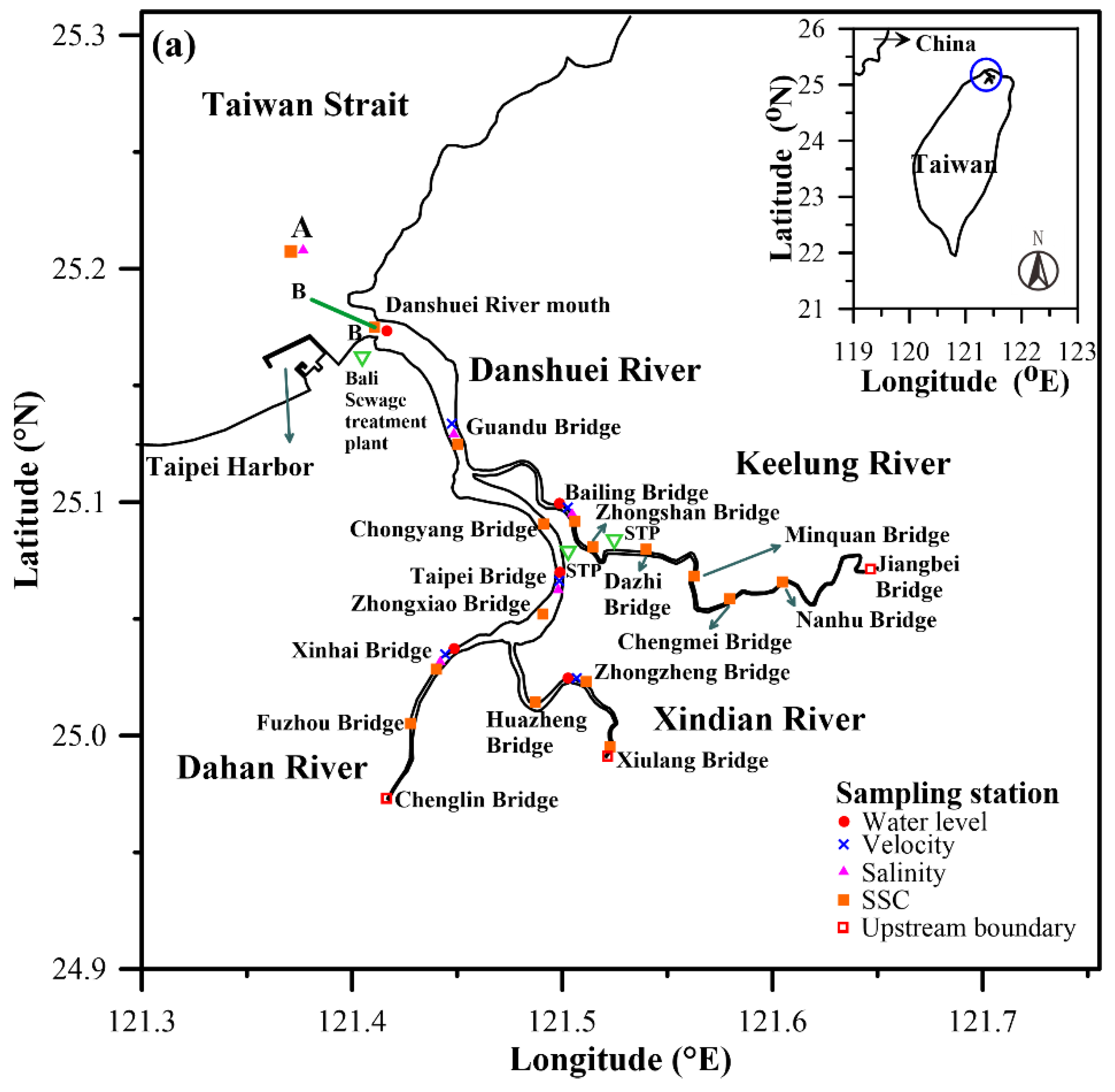
2. Study Area and Data

The Danshuei River in northern Taiwan has three major tributaries (the Dahan River, Xindian River, and Keelung River) to form a tidal estuarine system (see Figure 1a). With a watershed area of 2728 km2, the mean discharges of Dahan River, Xindian River, and Keelung River are about 38.99 m3/s, 69.72 m3/s, and 25.02 m3/s, respectively. The river with a total length of 327.6 km flows through four cities, i.e., Taipei City, New Taipei City, Taoyuan City, and Keelung City.
The Danshuei River has received a large amount of both treated and untreated domestic sewage water. There are three sewage treatment plants in this river system (Figure 1a). On the west bank of the river mouth, the Bali plant with sewage treatment capacity of 1.05 × 10⁶ m3/day is the largest one. The other two, located in the main Danshuei River and Keelung River, treat approximately 5.8 × 10⁵ m3 of sewage per day. In addition, sediment mainly from the upper reaches is flushed into the river during storms, yielding much higher SSC in the upstream region and gradually decreased SSC toward the mouth of the Danshuei River [47]. According to the annual report for environmental water quality monitoring issued by the Taiwan Environmental Protection Agency, the Danshuei River system has a certain degree of pollution, ranging from a slight to moderate level [45].
The downstream reaches of Danshuei River are influenced by tides and subjected to salt intrusion as it flows into the Taiwan Strait. The major tidal components are the principal lunar and solar semidiurnal tides, i.e., M2 and S2, respectively. The mean tidal range is about 2.22 m while the range can vary from 0.85 m to 3.1 m during the neap and spring tides [48,49]. In addition, there are two kinds of prevailing winds in Taiwan, i.e., the northeast wind in winter and southwest wind in summer.
In terms of the measurement data, bathymetry for the Danshuei River estuarine system and its adjacent coastal ocean (Figure 1b) are available from the Taiwan Water Resources Agency and the Taiwan Ocean Data Bank (supported by the Ministry of Science and Technology), respectively. Along the tidal portion of Danshuei River, cross-sectional profiles were obtained every 0.5 km (see http://www.wra10.gov.tw, accessed on 1 January 2022). In the adjacent coastal ocean, water depth with a uniform 200 m resolution was measured (see http://www.odb.ntu.edu.tw/en/, accessed on 1 January 2022). Furthermore, the measured water level, velocity, and salinity data over the same period were obtained from the Taiwan Water Resources Agency. In the upper reaches of three tributaries, suspended sediment concentration sampled by the Taiwan Environmental Protection Agency [50] were gathered and later used for model calibration and validation. The sampling stations for water level, velocity, salinity, and suspended sediment are also shown in Figure 1a.

3. Materials and Methods

3.1. Description of the 3D Hydrodynamic Model

The hydrodynamic modeling in this study was conducted using the semi-implicit cross-scale hydroscience integrated system model (SCHISM). SCHISM [51,52] is an open-source model which can be downloaded from the website. In recent years, SCHISM has been successfully applied to various areas with complex geometry and topography, including open and coastal oceans, tidal estuaries, rivers, and lakes [45,53,54,55,56,57,58,59,60].
SCHISM solves the Navier–Stokes equations and mass transport equation by a semi-implicit finite-volume/finite-element method based on unstructured grids in the horizontal plane and hybrid layers (S and Z) along the vertical direction. For the temporal scheme, the semi-implicit method is used to enhance numerical stability (associated with the Courant–Friedrichs–Lewy condition) since the errors have been alleviated in the mode-splitting approach. For spatial discretization, the finite element method is adopted to yield the horizontal velocities at the side centers while the finite volume method is applied to solve the vertical velocities at the element centers. Furthermore, a Eulerian–Lagrangian approach is utilized for the momentum advection. In terms of bathymetry, irregular bottom topography can be exactly fitted to avoid a staircase-like form if a special case of pure S-coordinate is chosen [61]. For turbulence closure (associated with vertical mixing), the generic length-scale k-kl model [62] is adopted. In the mass transport equation, salinity concentration is specified at the prism centers. In this study, water temperature was not considered in model simulations since there is no significant correlation between temperature and suspended sediment in the water body [49]. The readers can refer to Zhang et al. [51,52] for more detailed descriptions and solution procedures of SCHISM.

3.2. Suspended Sediment Model

The equations should be inserted in editable format from the equation editor. Suspended sediment can be linked with hydrodynamics, giving a coupled model SCHISM-SS. Basically, the time rate of change of suspended sediment is expressed using an advection–dispersion equation. Note that bottom exchanges (due to erosion flux E and deposition flux D) are also taken into account by the net sediment flux in the sea bed.
Bed erosion occurs when the bed shear stress exceeds a threshold of erosion. The bed erosion rate can be addressed by various empirical equations. Based on the concept of excess bottom shear stress [63], the bed parameterization of erosion rate is
E = M ( τ b τ c e 1 )   if   τ b > τ c e
  E = 0   if   τ b τ c e
where M denotes the erosion rate parameter; τ b represents the bottom shear stress, which can be calculated from the 3D hydrodynamic model (SCHISM); and τ c e denotes the critical shear stress for erosion.
Both erosion rate parameters and critical shear stress, which are closely dependent on the characteristics of sediment such as organic matter content, sediment composition, dry density, and water temperature [64,65], significantly affect the temporal and spatial variations of SSC. However, it is difficult to obtain their values in tidal estuaries from direct measurement. In general, these two parameters should be carefully determined during model calibration [22,66,67,68].
The deposition rate of suspended sediment can be estimated using the formula proposed in Einstein and Krone [69], i.e.,
  D = P w s C
where C denotes the concentration of suspended sediment, w s denotes the settling velocity, and P represents the probability of deposition and can be expressed in the following form [70], i.e.,
P = 1 τ b τ c d   if   τ b τ c d
P = 0   if   τ b > τ c d
To consider the effects of salinity and SSC on water density ( ρ ), the equation of state incorporated into the hydrodynamic model is expanded as
ρ = ρ w + C ρ s ( ρ s ρ w )
where ρ w denotes the salt water density and ρ s represents the sediment density.

3.3. Model Setup

For model setup, the computational mesh and water depth at the grid points were generated using the Surface-Water Modeling System (SMS) software (see the website https://www.aquaveo.com/software/sms-surface-water-modeling-system-introduction, accessed on 1 January 2022). As shown in Figure 1c, various grid sizes ranging from coarse (2.5 km) to fine (30 m) resolution were employed in the continental shelf and the river system, respectively, for the purpose of efficient and accurate modeling. Overall, the mesh consists of 20,448 elements and 11,433 nodes. In the vertical direction, the total water depth between sea bottom and free surface was divided into 10 uniform layers using a pure S coordinate. For all simulations, a fixed time step of 120 s was chosen to ensure numerical stability. A constant bottom roughness height of zo = 0.5 cm was specified.
To drive the hydrodynamic model, a time series of water level by superposition of five tidal constituents M2, S2, N2, K1, and O1 was specified at the ocean boundaries. In addition, the freshwater discharges measured during the same time period in 2016 were imposed at the upstream boundaries of Dahan River (at the Chenglin Bridge), Xindian River (at the Xiuiang Bridge), and Keelung River (at the Jiangbei Bridge). The salinities at the ocean and river upstream boundaries were specified to be 35 and 0 ppt, respectively. The initial water level, velocity, and salinity concentration were set to be 1.0 m, 0.5 m/s, and 15 ppt, respectively. A fifteen-day simulation was then conducted to reach an equilibrium state. For suspended sediment modeling, the measured SSCs were specified at upper reaches of three tributaries. At the ocean open boundaries, an averaged concentration of 5.0 mg/L commonly observed in the coastal sea was given.

3.4. Model Performance Evaluation

Four statistical indices were utilized to assess the performances of SCHISM-SS model during calibration and validation procedures, including the mean absolute error (MAE), root mean square error (RMSE), correlation coefficient (CC), and skill score (SSE). The CC and SSE can be expressed as
CC = i = 1 n [ ( X m ) i X m ¯ ] [ ( X o ) i X o ¯ ] i = 1 n [ ( X m ) i X m ¯ ] 2 i = 1 n [ ( X o ) i X o ¯ ] 2
SSE = 1 i = 1 n | ( X m ) i ( X o ) i | 2 i = 1 n [ | ( X m ) i X o ¯ | + | ( X o ) i X o ¯ | ] 2
where n is the total number of data;   ( X m ) i and X m ¯ represent the ith data point and the mean value for the modeled time series results, respectively; ( X o ) i and X o ¯ similarly follow the definitions above for the observed data. In general, better model performance can be indicated by a lower error (i.e., MAE and/or RMSE) and higher correlation (CC). Further, the range of SSE can be utilized to identify the model skills, i.e., below 0.2 for poor, 0.2 to 0.5 for good, 0.5 to 0.65 for very good, 0.65 to 1.0 for excellent, and 1.0 for perfect performance [71].

4. Model Calibration and Validation

To ensure the capability of simulating water level, velocity, salinity, and SSC, the SCHISM-SS model was rigorously calibrated and validated by comparison with the in situ measurement data during 2016. Note that the period of date for the following calibration and validation was based upon the availability of the data (e.g., the period of the field survey).

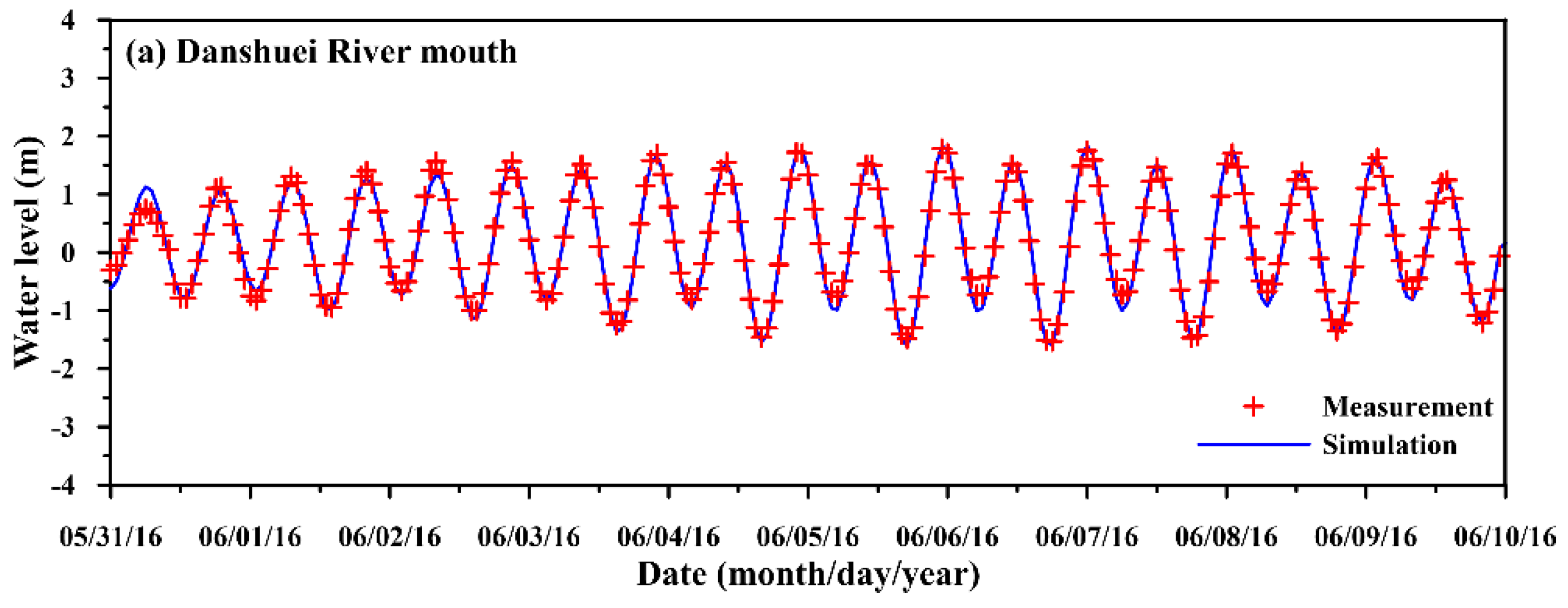
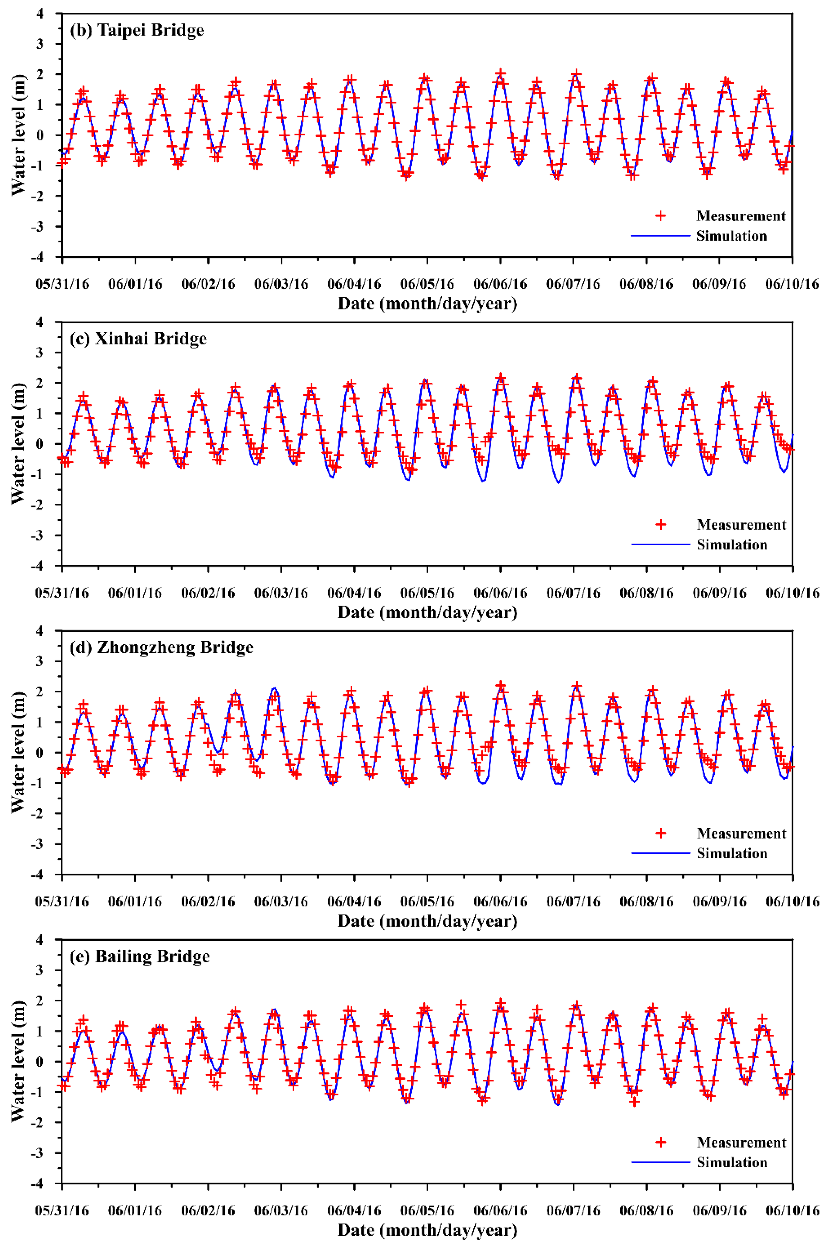
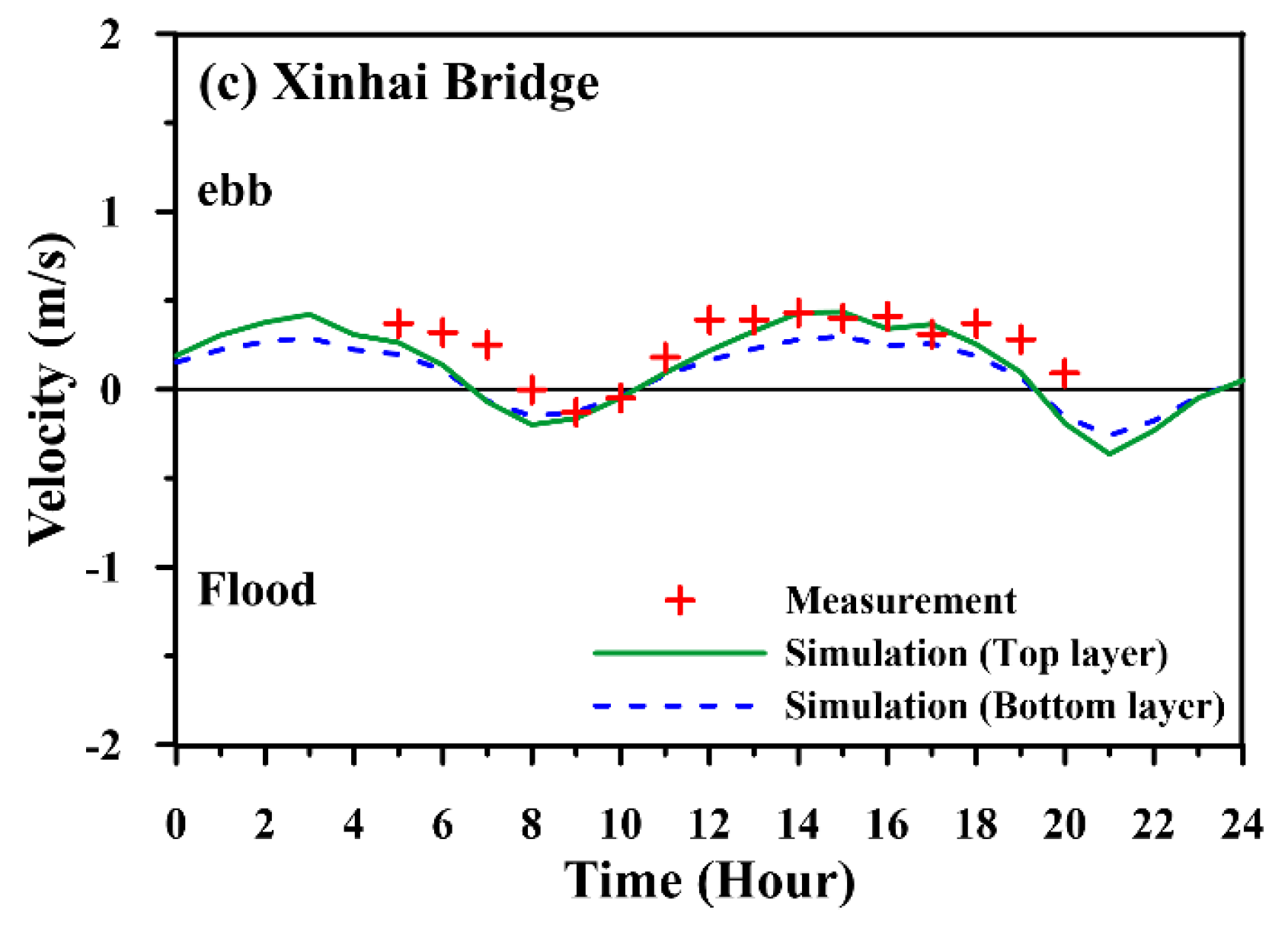
4.1. Calibration and Validation of the Hydrodynamic Model

The hydrodynamic model was first calibrated in terms of the water level for four seasons, i.e., from 28 February to 8 March, 31 May to 9 June, 3 to 12 September, and 3 to 12 December 2016. Figure 2 compares the time series of simulated and measured water levels at five gauge stations for the period from 31 May to 9 June 2016. From the river downstream to upstream, the periodic variations (between −1.0 m and 1.0 m) of the water levels owing to the tidal motion were well captured. Table 1 summarizes the statistical indices for model performance assessment in the four seasons, giving MAE, RMSE, and CC in a range from 0.057 m to 0.270 m, from 0.072 m to 0.354 m, and from 0.943 to 0.992, respectively. Furthermore, the skill score SSE up to 0.963 to 0.998 implies excellent performance of the hydrodynamic model.
Further, the hydrodynamic model was validated against the flow velocities, i.e., the velocity field in coastal ocean and the temporal variations of velocity in the estuary system. Figure 3 compares the observed and modeled surface velocity field in coastal sea during ebb tide period on 2 June 2016. The flow patterns of the observation and simulation results are in good agreement. Based upon the hourly measurement data on 4 July 2016, Figure 4 compares the temporal variation of depth-averaged velocity for five gauge stations. In general, the velocities (e.g., about 1.0 m/s at the Guandu Bridge during ebb tide) were accurately simulated, but were somewhat underestimated at the Bailling Bridge (see Figure 4e). The reason for such discrepancy is that the upstream boundary of Keelung River was given by its daily freshwater discharge (57.30 m3/s). Therefore, hourly variations in the flow velocity were not fully represented since the Bailling Bridge station is more susceptible to the influence from freshwater discharge. Table 2 presents the statistical indices to evaluate the model’s capability of simulating depth-averaged velocities. Among these five gauge stations, the ranges of MAE and RMSE are from 0.078 m/s to 0.282 m/s and from 0.087 m/s to 0.317 m/s, respectively. The values of CC and SSE range between 0.853–0.958 and 0.814–0.980, indicating excellent model performance for flow velocities.
Similarly, the model was validated with salinity in both coastal ocean and estuary systems. Figure 5 illustrates the surface salinity distribution in the coastal ocean during ebb tide period (on 2 June 2016) from simulations and observations. Qualitatively, the results are in reasonable agreement. Figure 6 compares depth-averaged salinity between the modeled results and measured data on 4 July 2016 for all gauge stations except for the Zhongzheng Bridge, where it was beyond the limit of salt intrusion. The variations of salinity over a tidal cycle (e.g., from 5 ppt to 25 ppt for the Guandu Bridge) were fairly presented in the simulation results. Similarly, some minor discrepancies are owing to the constant daily freshwater discharge applied at the upstream boundary. Model performances for the depth-averaged salinity at four stations are tabulated in Table 3. The ranges of MAE and RMSE are from 0.008 ppt to 3.729 ppt and from 0.011 ppt to 4.788 ppt at Guandu Bridge, Taipei Bridge, Xinhai Bridge, and Hsin-Hai Bridge, respectively. The values of CC and SSE are up to 0.892 and 0.928, except for those at the Hsin-Hai Bridge (due to the presence of limited salinity, i.e., 0.1 ppt). The model performance on salinity prediction is also excellent.

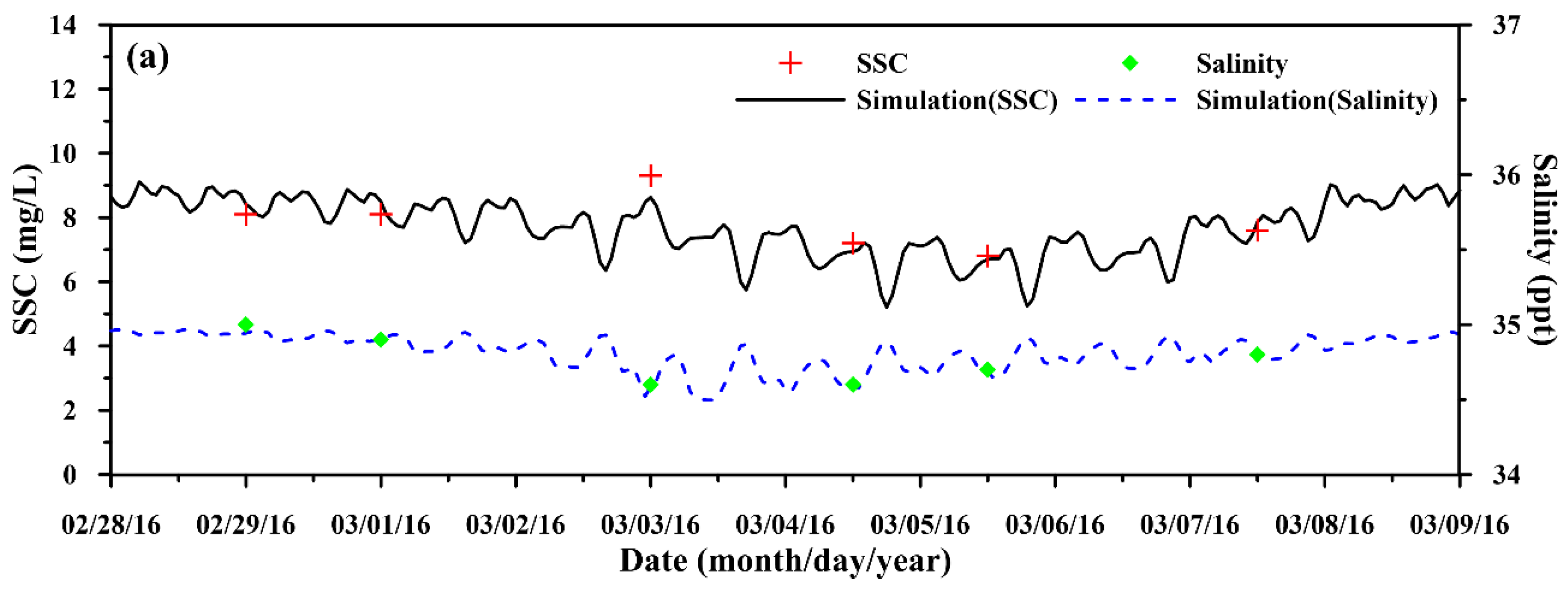
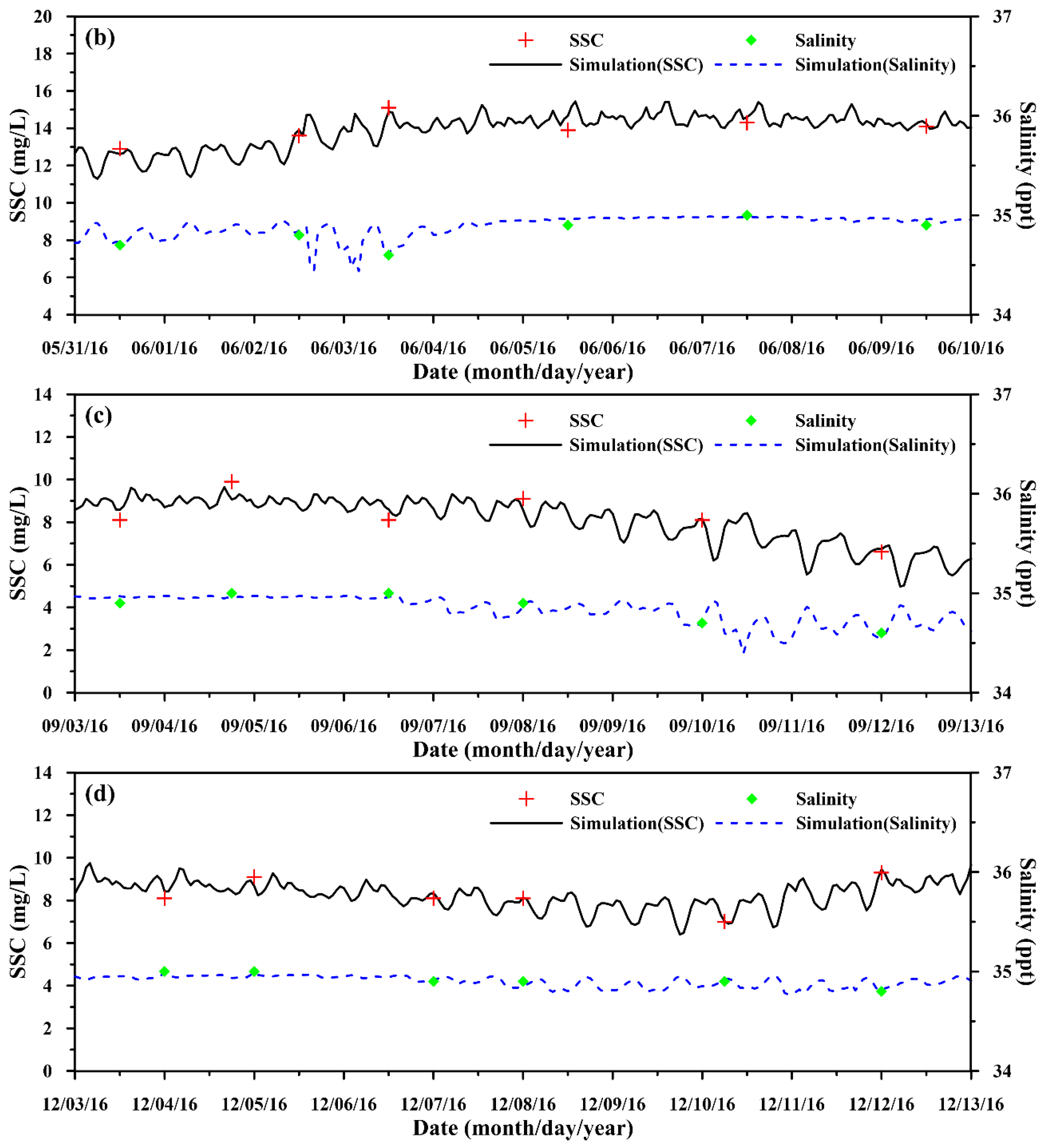
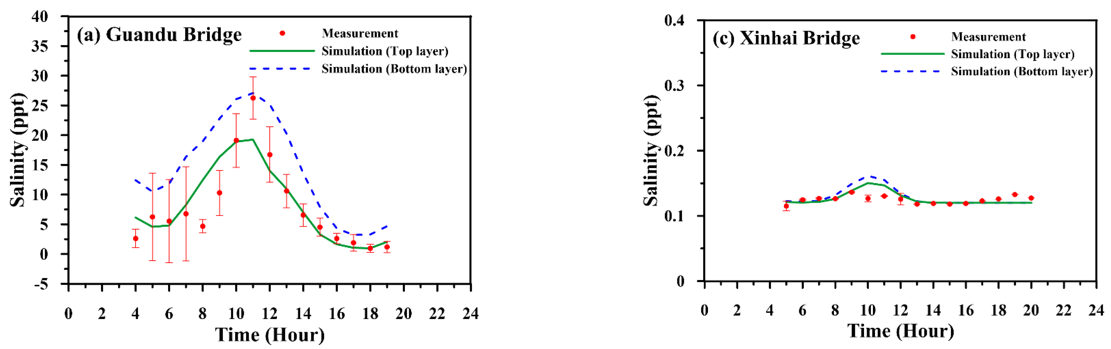
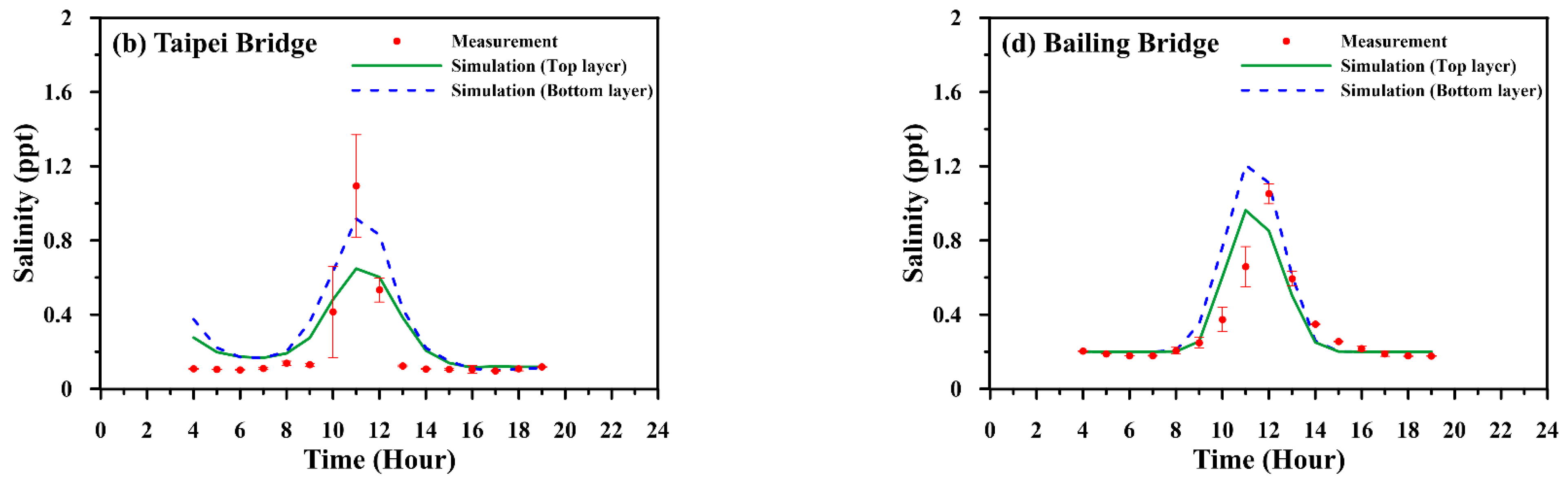
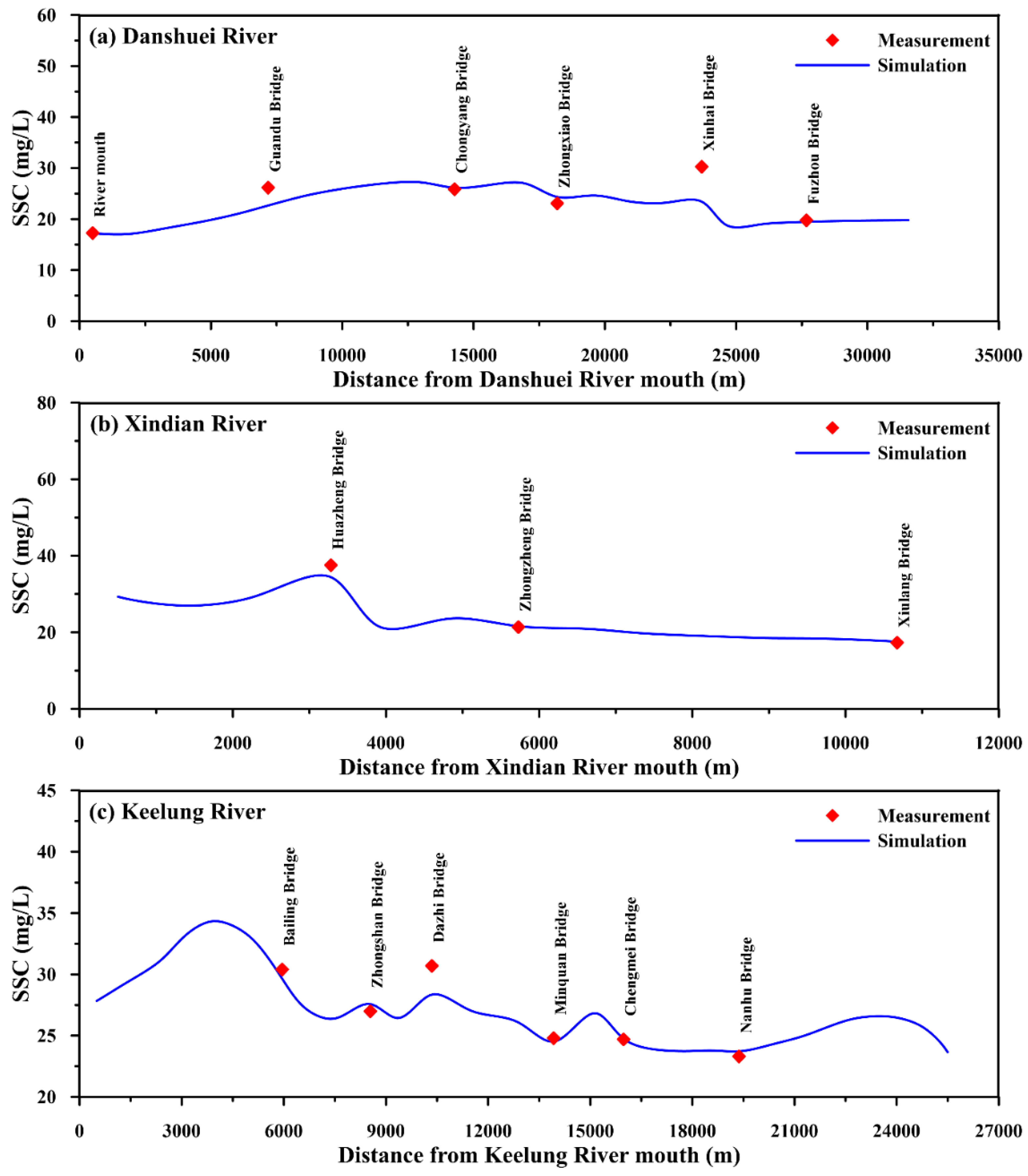
4.2. Calibration and Validation of Suspended Sediment Model

Subsequently, the suspended sediment module of the coupled model was calibrated and validated with the measured data (Mar. and Jun., 2016 for calibration; Sep. and Dec., 2016 for validation) to determine the parameters including the settling velocity ( w s ), critical shear stress for erosion ( τ c e ), critical shear stress for deposition ( τ c d ), and erosion rate ( M ). After model calibration, these parameters were fixed for further simulations (model validation).
For model calibration (2 June 2016), the concentrations of suspended sediment specified at upstream boundaries were 19.8 mg/L, 17.3 mg/L, and 23. 3 mg/L while the discharges were 29.61 m3/s, 622.77 m3/s, and 518.49 m3/s, respectively. Figure 7 shows the spatial variations of suspended sediment concentration along the mainstream and tributaries of the Danshuei estuarine system. In comparison with the measured data, the depth-averaged model results reproduce SSC distributions (in a range from 15 mg/L to 40 mg/L) reasonably well. The performance assessment results for both calibration and validation (covering wet and dry seasons, i.e., 2 Mar., 2 Jun., 6 Sep., and 6 Dec. 2016) together with the inflow discharges are presented in Table 4. The values of MAE and RMSE range from 0.392 mg/L to 3.818 mg/L and from 0.589 mg/L to 5.425 mg/L while the ranges of CC and SSE are between 0.750–0.999 and 0.770–0.999, respectively. Subsequently, sediment plume can be formed in coastal sea as turbidity waters flow out of the estuary. The depth-averaged results of suspended sediment concentration (as well as salinity) at Station A (see Figure 1a) are further compared in Figure 8. In both calibration and validation phases, the model faithfully addresses the movement of suspended sediment, e.g., higher concentrations (over 14 mg/L) in the coastal area during wet seasons (June 2016). The statistical indices for performance assessment are given in Table 5. For modeling SSCs in the continental shelf, the values of CC and SSE are above 0.83 and 0.92, respectively. Overall, as indicated by the skill scores, excellent performance for suspended sediment modeling along the river and in the coastal ocean has been achieved. Furthermore, the appropriate values of those parameters including the settling velocity ( w s ), critical shear stress for erosion ( τ c e ), critical shear stress for deposition ( τ c d ), and erosion rate ( M ) are set to 1.52 × 10⁻⁴ m/s, 2.5 N/m2, 0.5 N/m2, and 3 × 10⁻⁵ kg/m2·s, respectively.

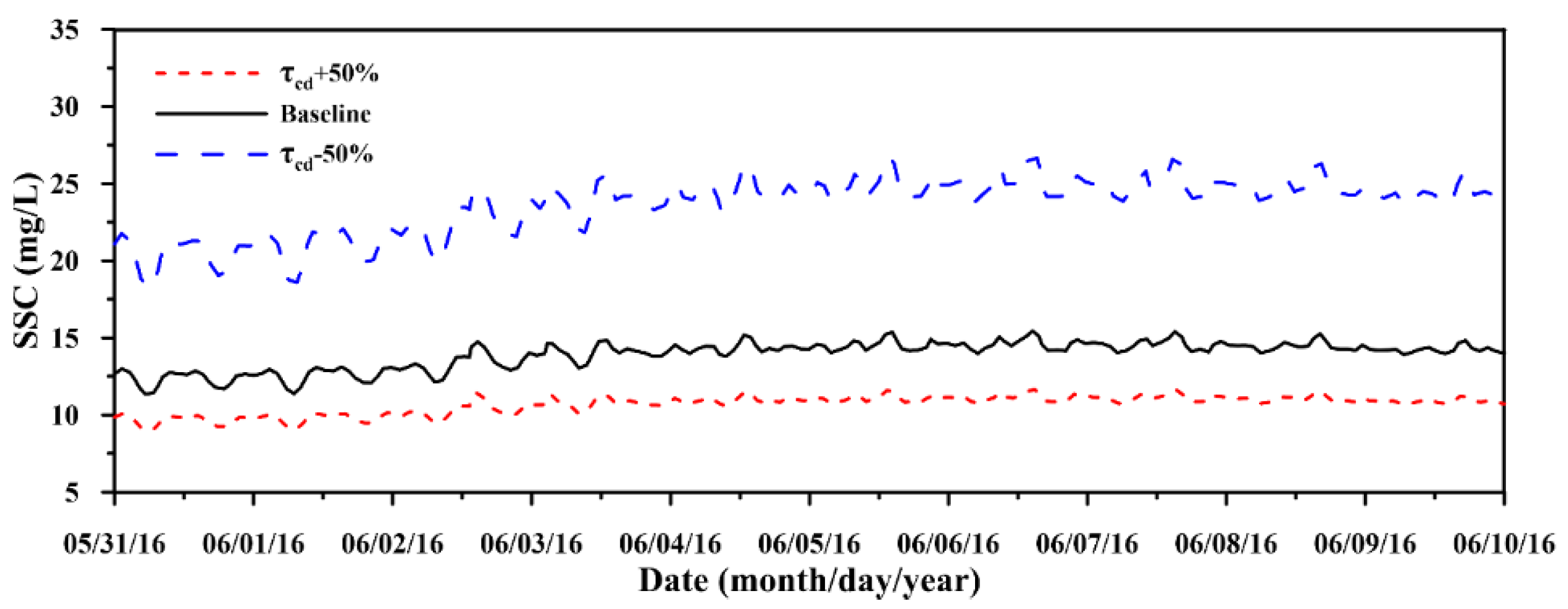
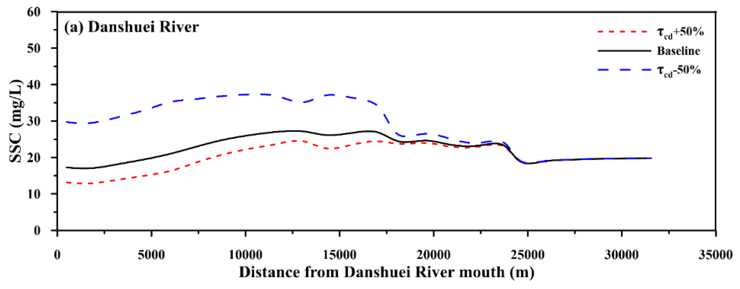
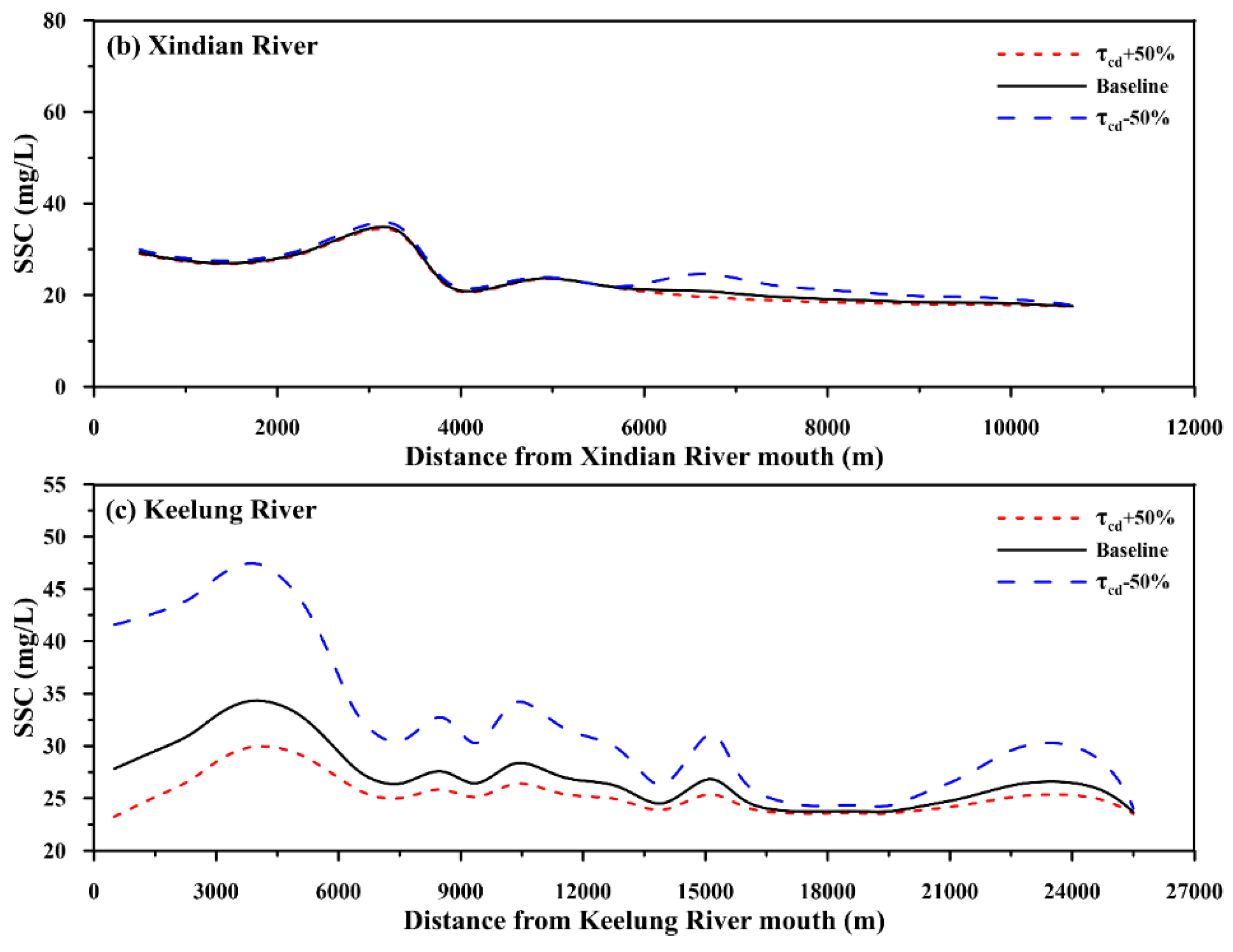
4.3. Sensitivity Analysis of the Suspended Sediment Model

A sensitivity analysis was further conducted to examine the effects of these four parameters and identify the most influential parameter on SSC modeling. The model simulation results in calibration (the date of 2 June 2016 for the tidal estuarine system and the period from 31 May to 9 June 2016 for the coastal region) were firstly adopted as the baseline. For the target parameter, an additional 50% increase or decrease to its original value was then applied to run the alternative case. The maximum change rate (MCR) was utilized to evaluate the sensitivity, i.e.,
MCR = C b a s e l i n e     C s a C b a s e l i n e × 100 %
where C b a s e l i n e and C s a denote the suspended sediment concentration for the baseline and for the sensitivity analysis, respectively.
For the sensitivity analysis, the changes of SSC in the tidal estuarine system and in the coastal region (Station A) due to the most influential parameter, i.e., the critical shear stress for deposition ( τ c d ), are presented in Figure 9 and Figure 10, respectively. Furthermore, the maximum change rates of SSC in response to 50% changes of four different parameters are summarized in Table 6. Note that the plus and minus values denote the increase and decrease in suspended sediment concentration, respectively. Among all the sensitivity tests, it is clear that the decrease in critical shear stress for deposition would yield the greatest increase in the SSC. The maximum change rates of SSC are 72.8%, 18.2%, 49.4%, and 73.6% in the Danshuei River–Dahan River, Xindian River, Keelung River, and coastal region (Station A), respectively.

5. Model Applications and Discussion

The validated SCHISM-SS was applied to examine the effects of environmental factors (including tidal forcing, salinity, river discharge, and wind shear stress) on the suspended sediment plumes in the continental shelf (local region) out of the Danshuei River. Note that extreme river discharges from upstream reaches were also considered since suspended sediment plumes would be affected by typhoons during summer seasons in Taiwan. In the following, each of the environmental factors was tested separately to identify its influence on suspended sediment plumes.

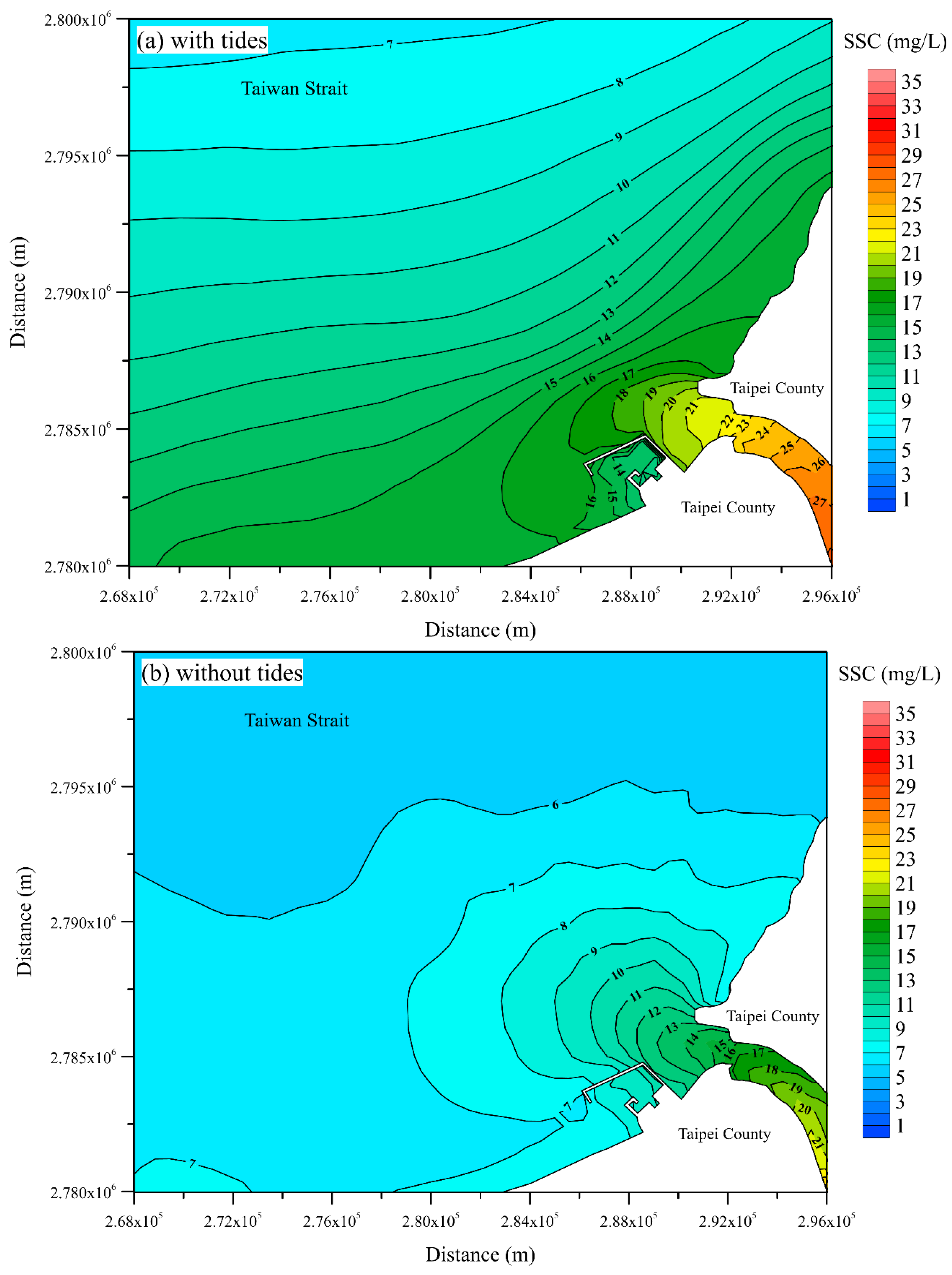
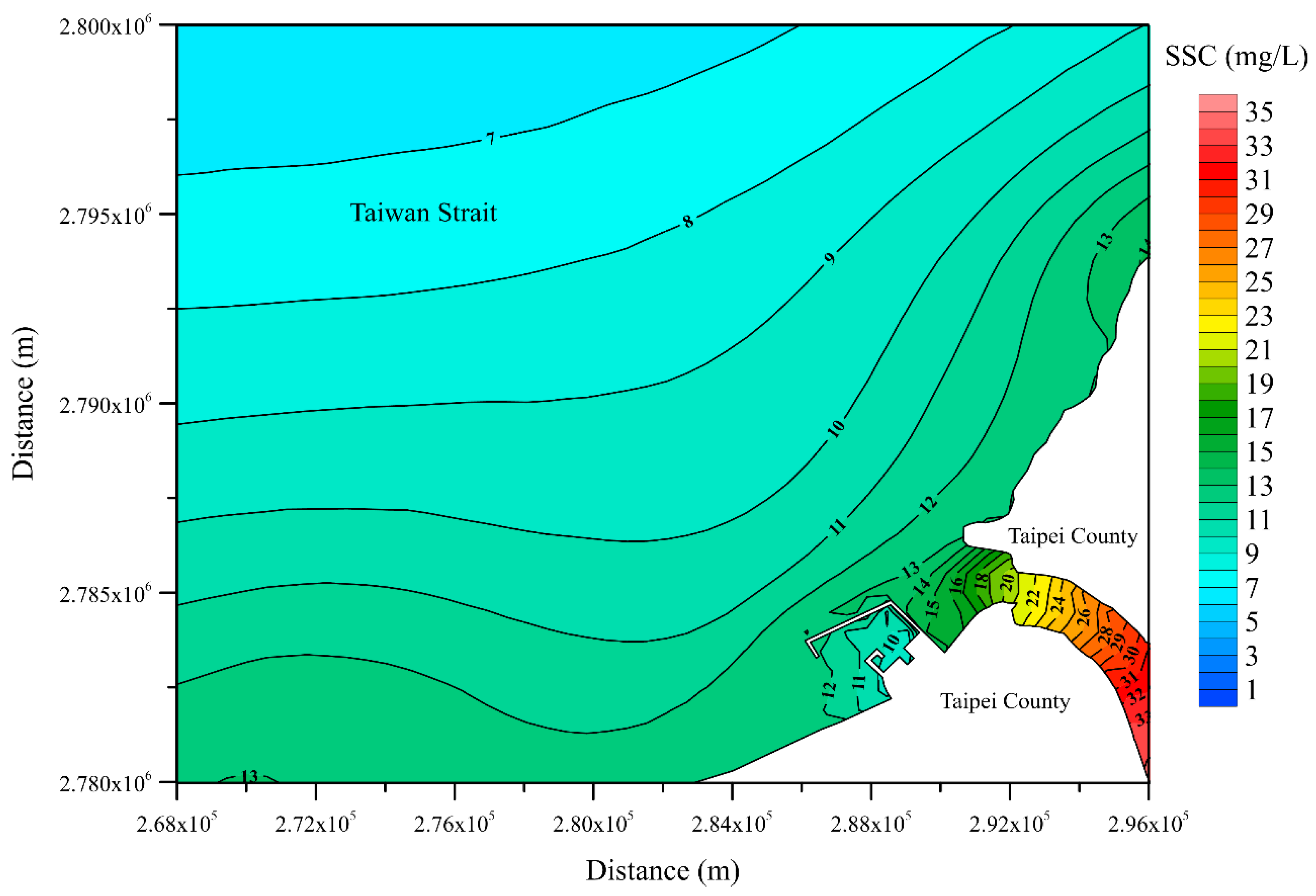
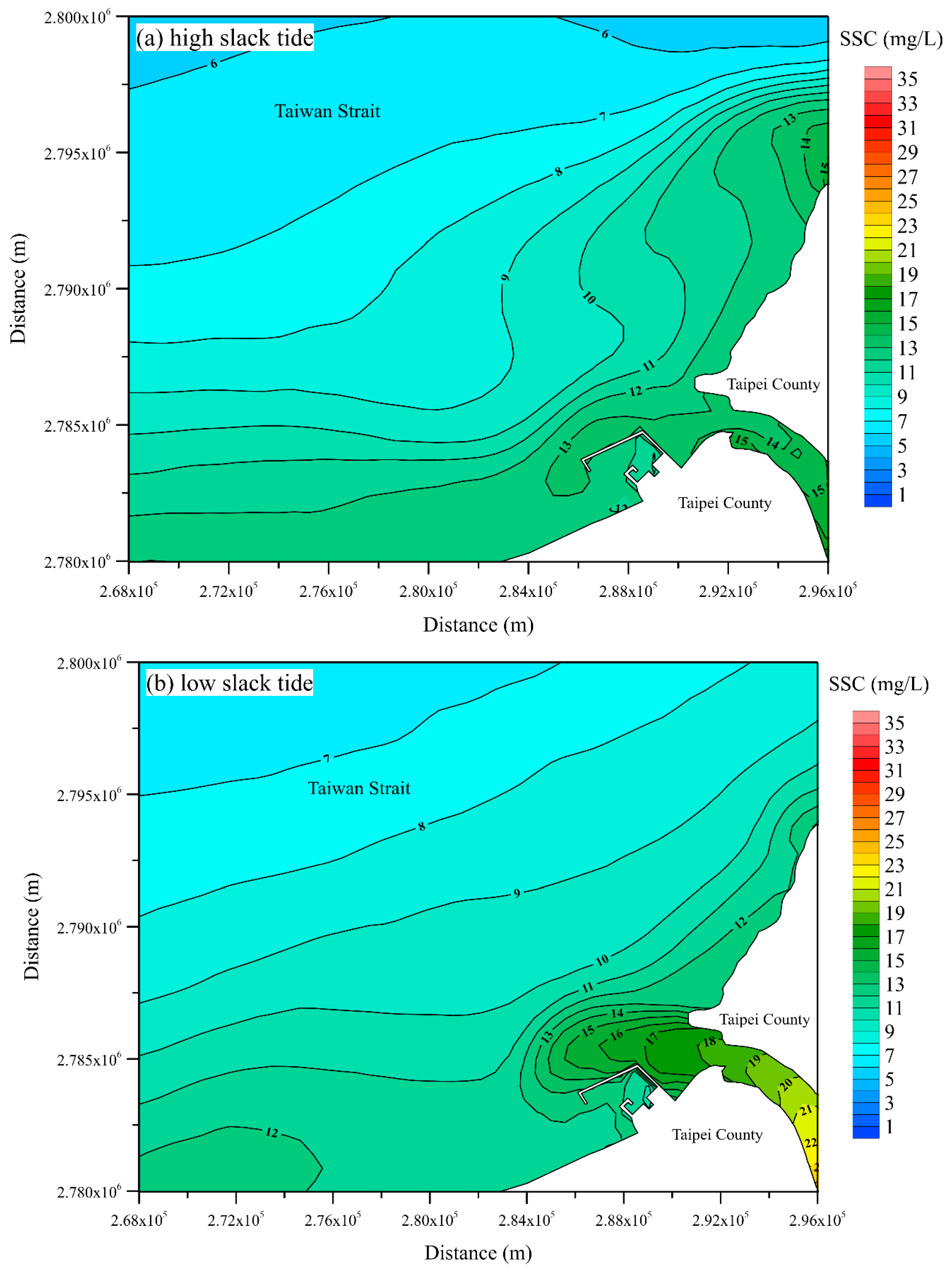
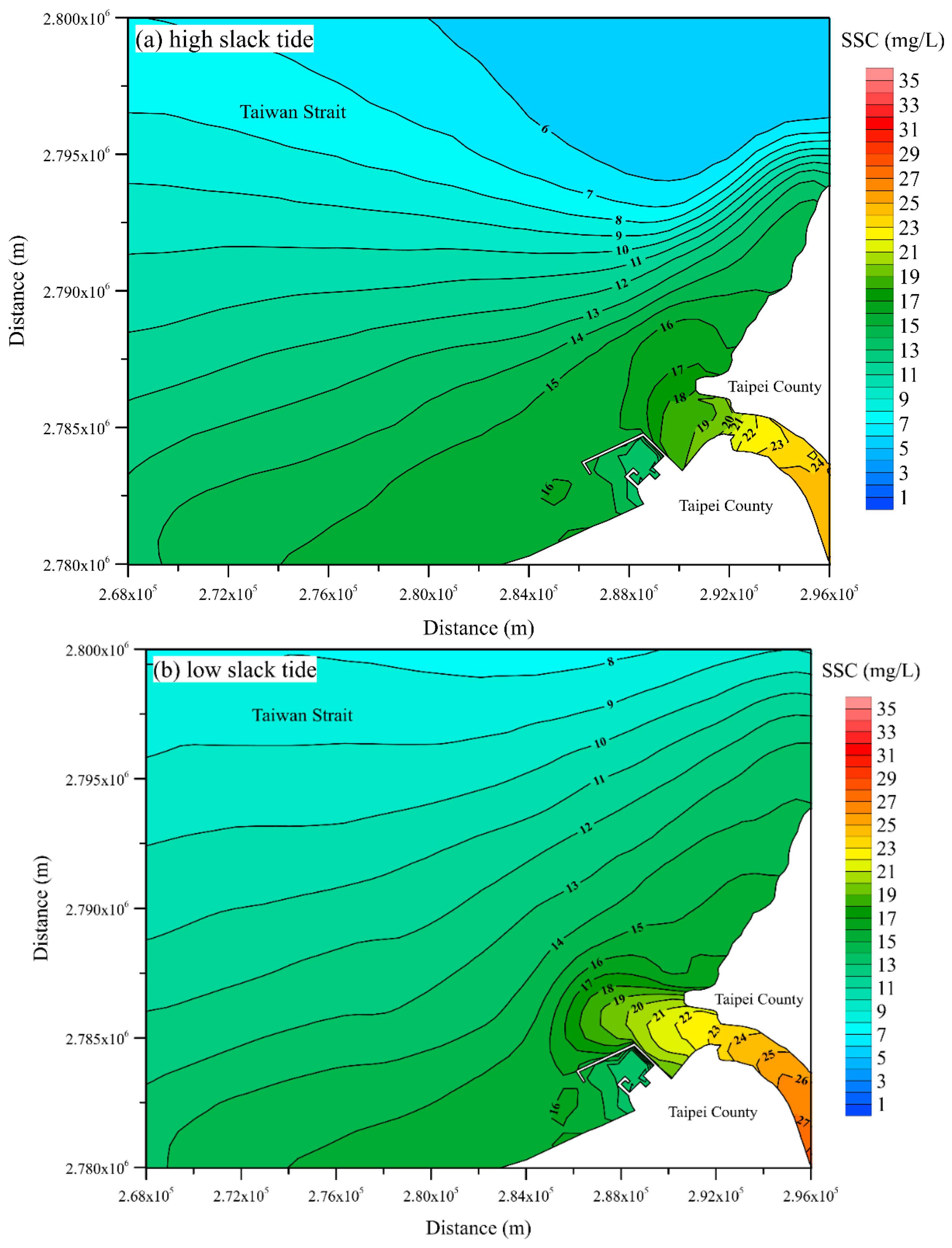
5.1. Effect of Tidal Forcing

Tidal forcing can be a dominating factor for the hydrodynamics and suspended sediment transport in both estuarine and coastal regions. Characteristics of suspended sediment plume under various tidal conditions (e.g., high and low slacks during spring or neap tide as well as no tidal motion) were investigated. The scenario simulations followed the same model setup, i.e., five major tidal constituents for open boundaries, except for mean freshwater discharges Qmean (29.18 m3/s, 60.84 m3/s, and 26.68 m3/s) and monthly averaged suspended sediment concentrations (16.55 mg/L, 27.78 mg/L, and 12.83 mg/L) specified at the upstream boundaries of three tributaries. Wind shear stress was excluded here.
The suspended sediment distributions at the surface layer during spring and neap tides are shown in Figure 11 and Figure 12 (with subplots (a) and (b) for the high and low slacks), respectively. Note that the tidal currents during flood (or ebb) tide would flow into (or out of) the study area from the north-eastern boundary. The variations of tidal currents with a large amount of seawater would greatly affect the concentrations of suspended sediments in the estuary and coastal areas through the mixing process, e.g., a higher (>15 mg/L) SSC close to the region just out of the river mouth at the ebb, low slack water (see Figure 11b). Further, the diffusion of suspended sediment also presents different distribution patterns due to tidal mixing, e.g., a wider range for suspended sediment with a concentration of 10 mg/L at the flood, high slack water (see Figure 11a). Overall, as indicated by the higher SSC (e.g., 13 mg/L) in the coastal area, more suspended sediment was conveyed from the estuary to the continental shelf at low slack for both spring and neap tides. Interestingly, the concentration of suspended sediment plume in the offshore region is higher during the neap tide. Again, notice that tidal mixing is the main mechanism in determining mass transport (of suspended sediment) in the tidal estuary and the continental shelf [20,72,73]. In other words, the weaker mixing is responsible for the higher SSC during the period of neap tide [71,74,75].
To further explore the influence of tides on suspended sediment plume, Figure 13 depicts both surface- and bottom-layer velocity fields after tidal-averaging procedures and Figure 14 shows tidally averaged surface-layer suspended sediment distributions for two scenarios (i.e., with and without the tidal actions). It is clear that the residual currents due to tide-induced barotropic circulation exist [21,76] and control the plume out of the Danshuei River estuary. Estimated by the plume area with SSC over 10 mg/L, the distance of plume from the mouth of the Danshuei River was utilized for characterization and discussion. The plume distances are 13.6 km and 5.3 km for the cases with and without tidal effects, respectively. Affected by the tidal motions, larger flux of suspended sediment from the Danshuei River estuary system (i.e., 2.32 × 10⁵ kg/day) leads to higher SSC and longer plume distance from the Danshuei River mouth. Overall, the effects of tidal motion on suspended sediment plume including tidal mixing as well as subtidal circulations in the estuary and coastal ocean are significant in the present study area.

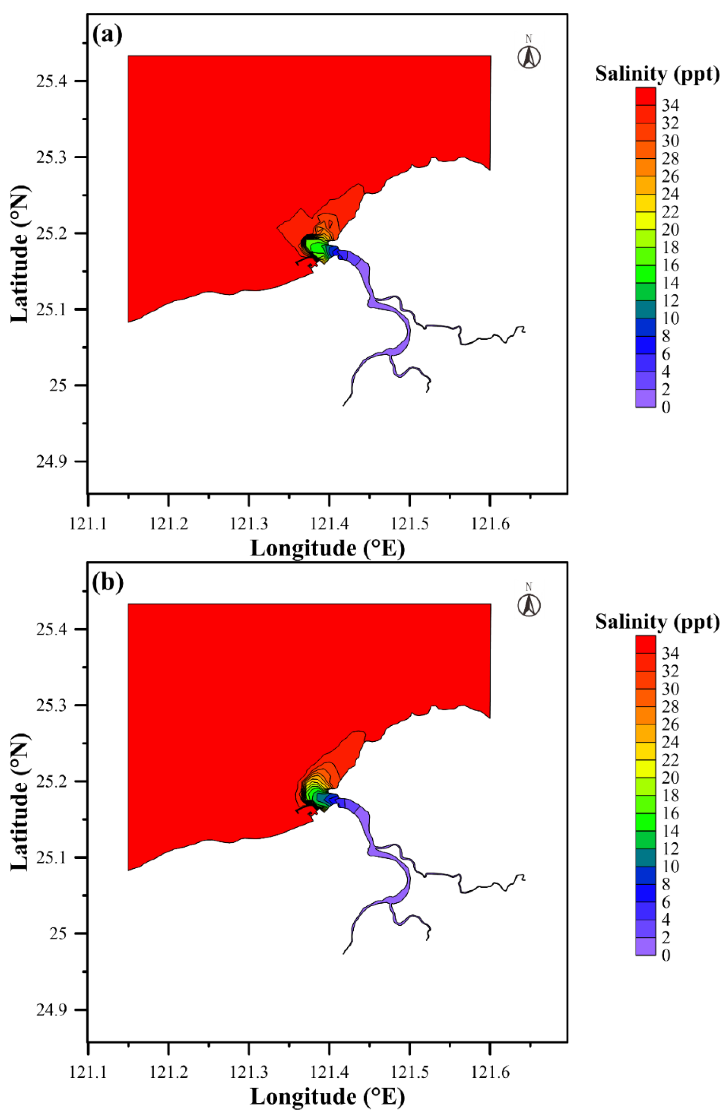
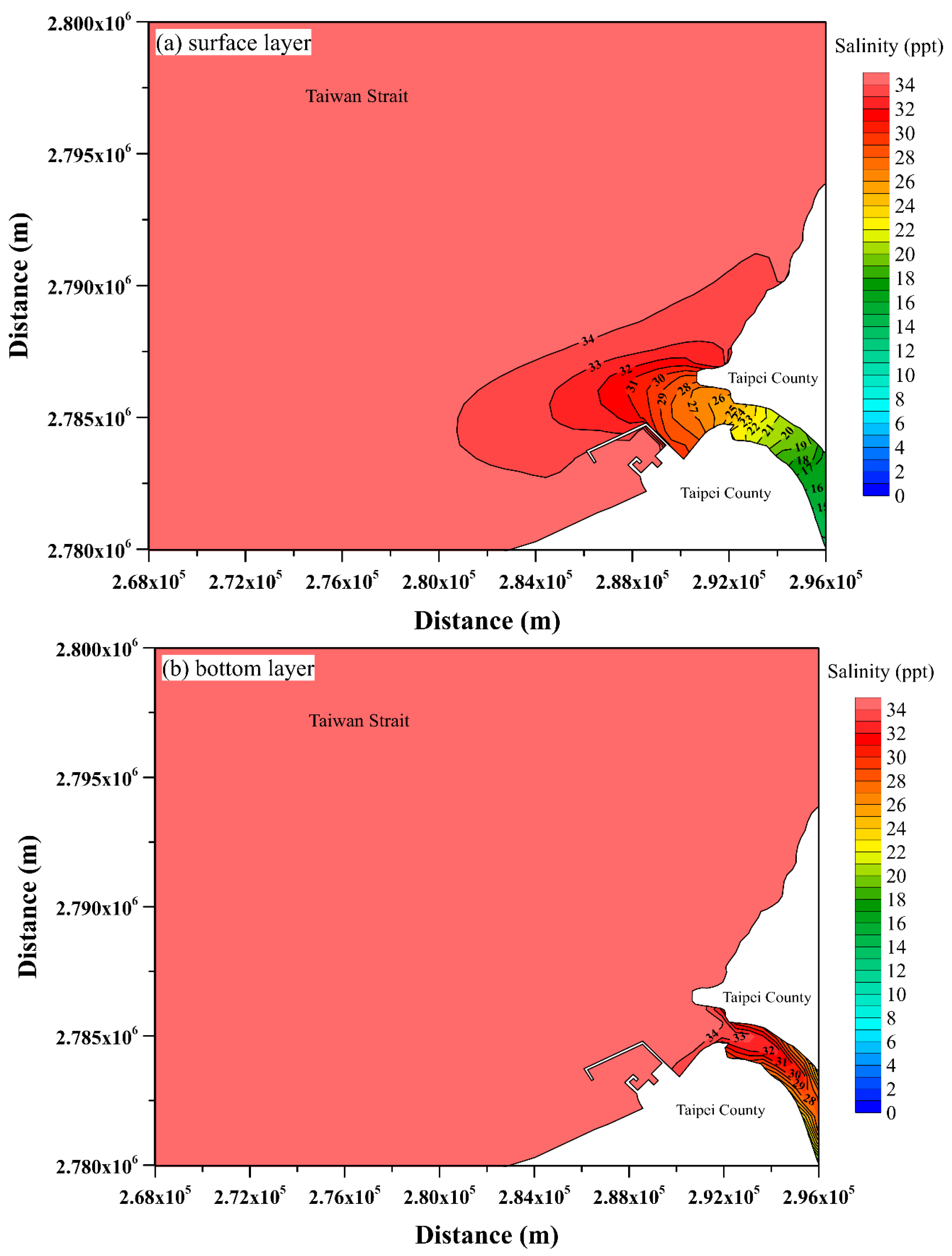
5.2. Effect of Salinity

Salinity might affect the spreads of suspended sediment plume over the continental shelf [24,25]. To clarify its potential influence on the plume dynamics in the Danshui River system, the model setup in the previous section was modified with a removal of salinity concentration (i.e., 0 ppt) along the open boundaries. The tidally averaged surface-layer suspended sediment distribution for this scenario (no salinity) is presented in Figure 15. Unlike the results (see Figure 14a) in Section 5.1, exclusion of salinity led to lower SSC and shorter plume distance out of the Danshuei River estuary.
The discrepancy between the simulated results (see Figure 14a and Figure 15) can be explained through examining the spatial distributions of tidally averaged surface- and bottom-layer salinity as well as the flow fields in the Danshuei River estuary and adjacent continental shelf (see Figure 16 and Figure 17). It can be seen that the surface concentration is lower than that at the bottom layer in the Danshuei River estuary when the salinity is present (see Figure 16a,b). As a consequence, the density difference due to the salinity of seawater would make the bottom-layer current flow upriver and surface-layer current flush toward the sea (see Figure 13a,b), forming a residual circulation that affects the transport of suspended sediment plume in the Danshuei River estuary (see Figure 14a). If no salinity exists, by contrast, no residual circulations were generated (see Figure 17) and lower SSCs near the river mouth were obtained. Overall, this scenario analysis clearly implies the importance of a salinity effect for the generation of gravitational currents and resultant suspended sediment distribution in the estuary and continental shelf [25,77].

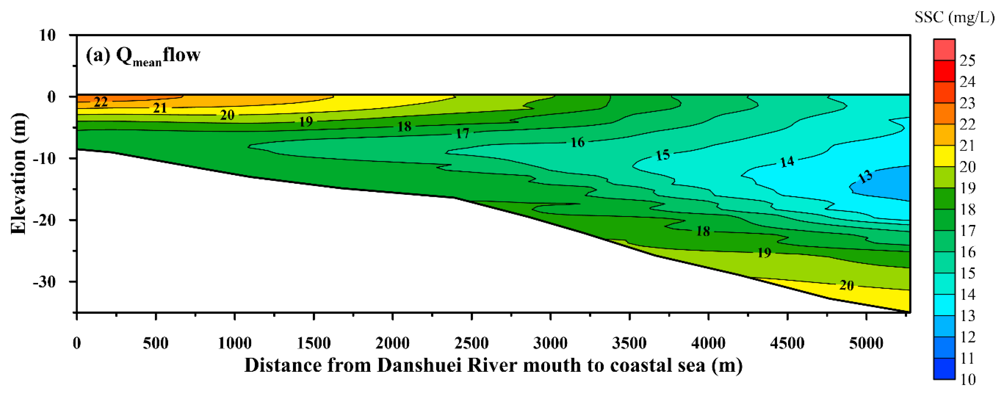
5.3. Effect of River Discharge

The discharge of turbidity river flow not only affects the salinity plume [2,7,8,10,14,27], but also plays an important role for the generation of suspended sediment plume in coastal regions [15,17,18,19]. Recently, the river plume of the Danshuei River and the influence from freshwater discharge were investigated (see [46]). This study further elucidated the effects of river discharge on the patterns of suspended sediment plume out of the Danshuei River estuary. Based upon the validated model, a scenario simulation was conducted with the modifications at upstream boundaries, i.e., an extreme flow condition which might take place during severe typhoon periods in Taiwan. According to our statistics analysis of the measurement data, the flowrates of a 10% exceedance probability Q10 are 64.78 m3/s, 131.36 m3/s, and 67.0 m3/s at the three tributaries. The extreme flow condition was given by Qe = 3Q10 in this study.
Figure 18 shows the tidally averaged suspended sediment plume for the extreme flow condition. In comparison to the results obtained by the mean flow condition (see Figure 14a), apparently, the suspended sediment plume was expanded (or pushed) further offshore with a plume distance of 20.5 km. The mechanism is the dramatically increased flux of suspended sediment (up to 1.64 × 10⁶ kg/day) due to a great amount of freshwater discharge into the Danshuei River mouth. Further, Figure 19 compares the vertical profiles of tidally averaged suspended sediment concentration along the B-B section (Figure 1a). As can be seen, the extreme flow causes a suspended sediment plume with a larger extent and higher concentration in the upper surface portion of the coastal ocean. Overall, the river discharge has a crucial effect on the distance of suspended sediment plumes in coastal regions.

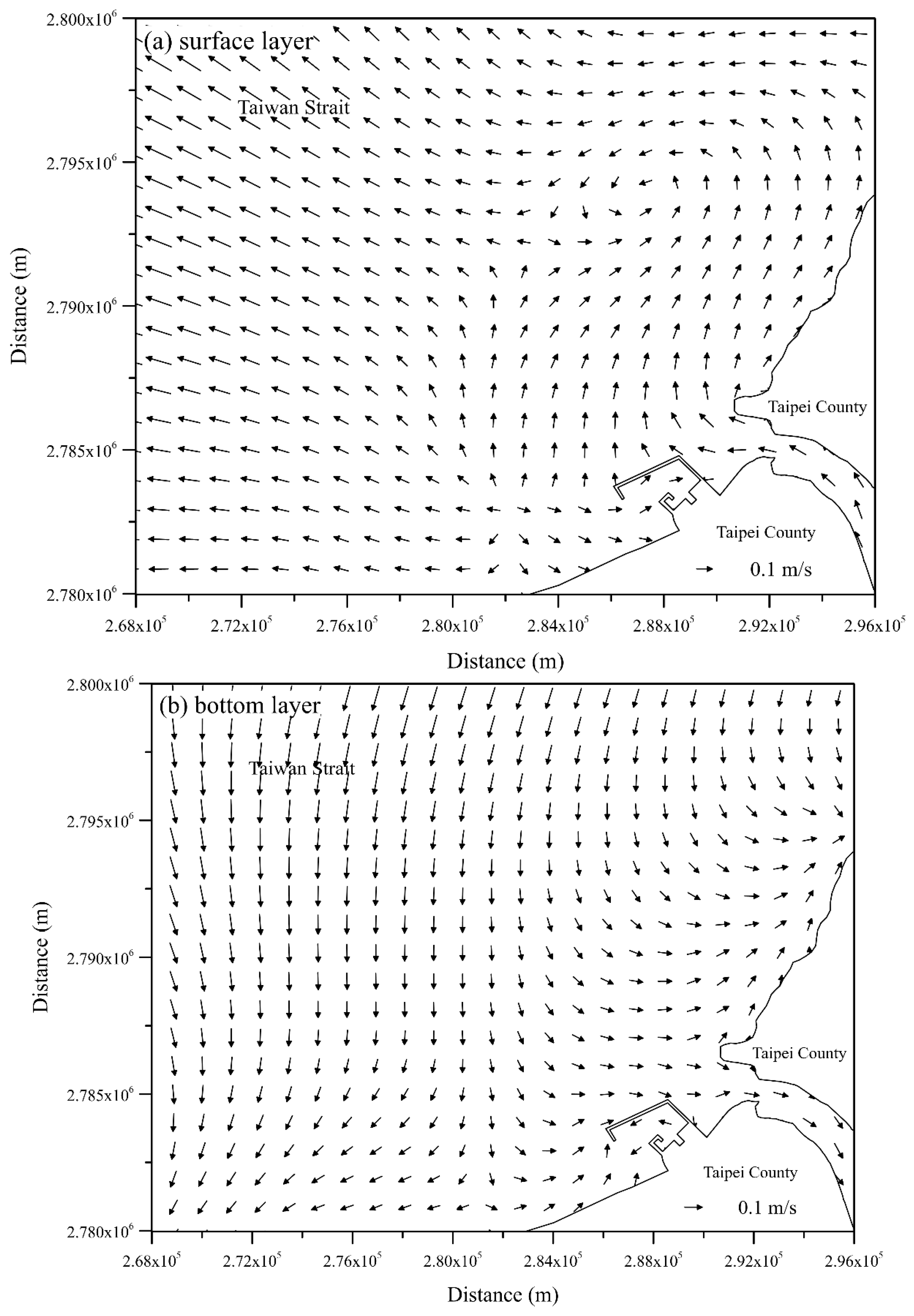
5.4. Effects of Wind Stress

Wind shear stress (determined by wind direction and speed) is also an influential factor to the plume characteristics on the continental shelf [9,10,26,27]. In addition to those environmental factors in previous sections (i.e., tidal forcing, salinity, mean river flow), the wind forcing was also taken in account in model simulations. Another two scenarios representing the major prevailing wind (in northeast and southwest directions) at a speed of 15 m/s were conducted. The nondimensional Wedderburn number W [78] is used to evaluate the relative contributions between wind forcing and buoyancy effect on the river plume, i.e.,
W = τ w L Δ ρ g H 2
where g represents the gravitational acceleration, H indicates the mean water depth, L denotes the distance from the river mouth to the offshore area of the sediment plume, τ w represents the wind stress, and Δ ρ is the density change.
Figure 20 illustrates the distributions of SSC under the actions of northeast and southwest prevailing winds. Meanwhile, Table 7 summarizes the Wedderburn numbers for various scenarios including wind directions (northeast and southwest), wind speeds (6 and 15 m/s), and different river discharges (Qmean and 3Q10 flows). When the strong prevailing winds (i.e., wind speed of 15 m/s in northeast and southwest directions) occur, the Wedderburn number with a value greater than 1 (W > 1) implies that the wind forcing would take control of the suspended sediment plume. In particular, the suspended sediment plume is dominated by the large wind stress no matter whether it is under the mean (Qmean) or extreme (3Q10) flow condition. Thus, the directions of prevailing winds (i.e., northeast and southwest) cause the slightly southward and northward suspended sediment plumes, respectively. Compared to the results in no wind condition (see Figure 14a), the movement of suspended sediment plume was mainly confined to the river mouth. Note that the suspended sediment plume becomes buoyancy-controlled when the wind speed is under 6 m/s. Overall, our findings for the wind effects on suspended sediment plume are similar and consistent with those in the literature (e.g., [3,79,80,81,82,83]).

5.5. Limitations and Future Directions

In this article, we presented an investigation on suspended sediment plumes out of the Danshuei River estuary and its responses to various environmental forcing factors. The topic of the present study is interesting and quite important with a general concern for understanding the estuary dynamics. A coupled three-dimensional hydrodynamic and suspended sediment transport model was adopted as an efficient tool for the purpose of assessing suspended sediment plumes along the estuary to the continental shelf. In the previous sections, a systematic research framework was utilized to measure the environmental implications (e.g., the impacts from tidal forcing, salinity, river runoff, and wind forcing). Overall, the results were reasonably reproduced and consistent with those made in earlier studies.
Some limitations (with respect to the numerical modelling) in this study should be noted. The (physical) parameters used for addressing critical stresses are of critical importance for the spatial and temporal distribution of suspended sediment. However, it is not feasible to determine the parameters through field measurement. Thus, careful selection of parameters in the process of model calibration and validation is essential [67,84]. Note that a trial-and-error procedure with a rigorous comparison against available measurement data is often required for selecting proper parameters. While the model calibration and validation were carried out, some discrepancy still exists subject to the limitations of measured velocity, salinity, and suspended sediment concentration in the estuarine system and coastal sea. Regular in situ observations and field surveys for detailed data collection would be beneficial [38,66,85].
In future work, the coupled model can be further expanded to include water quality, bacteria, and heavy metals to gain a deeper insight into pollutants in the estuary and coastal ocean. Differential transport of sediment particles of various sizes (or densities) not considered in the present study can be investigated [86]. In addition, as one of the most important extreme events affecting Taiwan and the Taiwan Strait, typhoons that cause short-term environmental dynamic changes generate large wind-induced waves or storm surges [87], impacting the suspended sediment transport in the estuary and adjacent coastal area. A wave model (e.g., WW3) will be also implemented with the SCHISM-SS to include those processes. Overall, this study has revealed the “from source to sink” process of river sediment discharged into the sea. More results and analysis for the relevant processes, mechanisms, and new insights will be reported in the near future.

6. Conclusions

The effects of environmental factors upon the suspended sediment plumes out of the Danshuei River estuary were investigated using an unstructured-grid three-dimensional hydrodynamic model (SCHISM) coupled with a model of suspended sediment (SS). The SCHISM-SS model was calibrated and validated against the in situ measurement data from 2016. As implied by four statistical indices (MAE, RMSE, CC, and SSE), model results reproduced the water levels, velocities, salinities, and suspended sediment concentrations satisfactorily. In addition, the sensitivity analysis indicated that the critical shear stress for deposition was most influential.
The validated SCHISM-SS model was then applied to explore the significant role of various environmental factors in the dynamics of suspended sediment plumes from the estuary to its adjacent coastal sea, including tidal forcing, salinity, river discharge, and wind stress. The findings of this study are summarized as follows.
(1) In terms of tidal effects, the results revealed that more suspended sediment was conveyed from the estuary to the continental shelf at low slack water. The concentration of suspended sediment plume in the offshore region is higher during the neap tide owing to stronger tidal mixing. Estimated by the plume area with SSC over 10 mg/L, the plume distance from the mouth of the Danshuei River was used for further characterization. Affected by tidal motions, larger flux of suspended sediment from the Danshuei River estuary system would lead to higher SSC and longer plume distance (13.6 km).
(2) Further, by means of salinity exclusion, the model results clearly showed that the density difference due to salinity of seawater makes the bottom-layer current flow upriver and surface-layer current flush toward the sea, forming a residual circulation and spreading more suspended sediment in the Danshuei River estuary.
(3) An extreme flow condition (Qe = 3Q10) which might take place during severe typhoon periods in Taiwan was considered. Apparently, due to a great amount of freshwater discharge, the flux of suspended sediment at the Danshuei River mouth was dramatically increased to 1.64 × 10⁶ kg/day. Hence, the suspended sediment plume was expanded further offshore with a plume distance about 20.5 km. Furthermore, the extreme flow caused the suspended sediment plume with a larger extent and higher concentration in the upper portion of the coastal ocean.
(4) The strong prevailing wind would confine the suspended sediment plume to the mouth of the Danshuei River. The wind directions (northeast and southwest) would lead to slightly southward and northward suspended sediment plumes, respectively. Furthermore, by the implication of the Wedderburn number, the suspended sediment plume in the study area would be dominated by strong winds (i.e., 15 m/s) regardless of being under mean (Qmean) or extreme (3Q10) flow conditions. As the wind speed is below 6 m/s, on the other hand, the suspended sediment plume would be buoyancy-controlled.
(5) Overall, the main conclusion in this study is that among the environmental factors, river discharge is most influential to the suspended sediment plume on the continental shelf out of Danshuei River.

Author Contributions

Conceptualization, W.-C.L., H.-M.L. and C.-C.Y.; methodology, W.-C.L. and C.-C.Y.; validation, H.-M.L.; formal analysis, W.-C.L., H.-M.L. and C.-C.Y.; investigation, W.-C.L., H.-M.L. and C.-C.Y.; resources, W.-C.L.; writing—original draft preparation, W.-C.L., H.-M.L. and C.-C.Y.; writing—review and editing, W.-C.L., H.-M.L. and C.-C.Y.; visualization, H.-M.L.; supervision, W.-C.L. and C.-C.Y.; project administration, W.-C.L.; funding acquisition, W.-C.L. All authors have read and agreed to the published version of the manuscript.

Funding

This research was funded by Ministry of Science and Technology, Taiwan, under grant number 107-2625-M-239-002.

Institutional Review Board Statement

Not applicable.

Informed Consent Statement

Not applicable.

Data Availability Statement

Not applicable.

Acknowledgments

This study was provided by the Ministry of Science and Technology (MOST), Taiwan. The authors sincerely express their great appreciation to the Taiwan Water Resources Agency, Central Weather Bureau, and Environmental Protection Administration for providing valuable data. The authors also appreciate Y. Zhang at VIMS, College of William and Mary for providing the SCHISM source code.

Conflicts of Interest

The authors declare no conflict of interest.

References

  1. Perianez, R. Modelling the transport of suspended particulate matter by the Rhone River plume (France): Implications for pollutant dispersion. Environ. Pollut. 2005, 133, 351–364. [Google Scholar] [CrossRef]
  2. Liste, M.; Grifoll, M.; Monbaliu, J. River plume dispersion in response to flash flood events: Application to the Catalan shelf. Cont. Shelf Res. 2014, 87, 96–108. [Google Scholar] [CrossRef]
  3. Schiller, R.V.; Kourafalou, V.H.; Hogan, P.; Walker, N.D. The dynamics of the Mississippi River plume: Impact of topography, wind and offshore forcing on the fate of plume waters. J. Geophys. Res. 2011, 116, C06029. [Google Scholar] [CrossRef]
  4. MacCready, O.; Banas, N.S.; Hickey, B.M.; Dever, E.P.; Liu, Y. A model study of tide- and wind-induced mixing in the Columbia River Estuary and plume. Cont. Shelf Res. 2009, 29, 278–291. [Google Scholar] [CrossRef]
  5. Marques, W.C.; Fernandes, E.H.; Monteiro, I.O.; Moller, O.O. Numerical modeling of the Patos Lagoon coastal plume, Brazil. Cont. Shelf Res. 2009, 29, 556–571. [Google Scholar] [CrossRef]
  6. Sousa, M.C.; Vaz, N.; Alvarez, I.; Gomez-Gesteira, M.; Dias, J.M. Modeling the Minho River plume intrusion into the Rias Baixas (NW Iberian Peninsula). Cont. Shelf Res. 2014, 85, 30–41. [Google Scholar] [CrossRef]
  7. Androulidakis, Y.S.; Kourafalou, V.H.; Schiller, R.V. Process studies on the evolution of the Mississippi River plume: Impact of topography, wind and discharge conditions. Cont. Shelf Res. 2015, 107, 33–49. [Google Scholar] [CrossRef]
  8. Vallaeys, V.; Karna, T.; Delandmeter, P.; Lambrechts, J.; Baptista, A.M.; Deleersnijder, E.; Hanert, E. Discontinuous Galerkin modeling of the Columbia River’s coupled estuary-plume dynamics. Ocean Model. 2018, 124, 111–124. [Google Scholar] [CrossRef]
  9. Zhao, J.; Gong, W.; Shen, J. The effect of wind on the dispersal of a tropical small river plume. Front. Earth Sci. 2018, 12, 170–190. [Google Scholar] [CrossRef]
  10. Yu, X.; Guo, X.; Morimoto, A.; Buranapratheprat, A. Simulation of river plume behaviors in a tropical region: Case study of the Upper Gulf of Thailand. Cont. Shelf Res. 2018, 153, 16–29. [Google Scholar] [CrossRef]
  11. Osadchiev, A.; Sedakov, R.; Barymova, A. Response of a Small River Plume on Wind Forcing. Front. Mar. Sci. 2021, 8, 809566. [Google Scholar] [CrossRef]
  12. Zhi, H.; Wu, H.; Wu, J.; Zhang, W.; Wang, Y. River Plume Rooted on the Sea-Floor: Seasonal and Spring-Neap Variability of the Pearl River Plume Front. Front. Mar. Sci. 2022, 9, 791948. [Google Scholar] [CrossRef]
  13. Osadchiev, A.A.; Zavialov, P.O. Lagrangian model of a surface-advected river plume. Cont. Shelf Res. 2013, 58, 96–106. [Google Scholar] [CrossRef]
  14. Zheng, S.; Guan, W.; Cai, S.; Wei, X.; Huang, D. A model study of the effects of river discharges and interannual variation of winds on the plume front on winter in Pear River Estuary. Cont. Shelf Res. 2014, 73, 31–40. [Google Scholar] [CrossRef]
  15. Yao, H.Y.; Leonardi, N.; Li, J.F.; Fagherazzi, S. Sediment transport in a surface-advected estuarine plume. Cont. Shelf Res. 2016, 116, 122–135. [Google Scholar] [CrossRef]
  16. Kashyap, S.; Dibike, Y.; Shakibaeinia, A.; Prowse, T.; Droppo, I. Two-dimensional numerical modelling of sediment and chemical constituent transport within the lower reaches of the Athabasca River. Environ. Sci. Pollut. Res. 2017, 24, 2286–2303. [Google Scholar] [CrossRef]
  17. Cheng, P.; Li, M.; Li, Y. Generation of an estuarine sediment plume by a tropical storm. J. Geophys. Res. 2013, 118, 856–868. [Google Scholar] [CrossRef]
  18. Fissel, D.B.; Lin, Y.; Scoon, A.; Lim, J.; Brown, L.; Clouston, R. The variability of the sediment plumes and ocean circulation features of the Nass River Estuary, British Columbia. Satell. Oceanogr. Meteorol. 2017, 2, 1–15. [Google Scholar] [CrossRef]
  19. Luo, Z.; Zhu, J.; Wu, H.; Li, X. Dynamics of the sediment plume over the Yangtz Bank in the Yellow and East China Seas. J. Geophys. Res. 2017, 122, 10073–10090. [Google Scholar] [CrossRef]
  20. Whitney, M.M.; Garvine, R.W. Simulating the Delaware Bay buoyant outflow: Comparison with observations. J. Phys. Oceanogr. 2006, 36, 3–21. [Google Scholar] [CrossRef]
  21. Tarya, A.; Hoitink, A.J.F.; Van der Vegt, M. Tidal and subtidal flow patterns on a tropical continental shelf semi-insulated by coral reefs. J. Geophys. Res. 2010, 115, C09029. [Google Scholar] [CrossRef]
  22. Van, C.P.; Gourgue, O.; Sassi, M.; HoitinkTon, A.J.F.; Deleersnijder, E.; Soares-Frazao, S. Modelling fine-grained sediment transport in Mahakam land-sea continuum, Indonesia. J. Hydro-Environ. Res. 2016, 13, 103–120. [Google Scholar]
  23. Guo, K.; Zou, T.; Jiang, D.; Tang, C.; Zhang, H. Variability of Yellow River turbidity plume detected with satellite remote sensing during water sediment regulation. Cont. Shelf Res. 2017, 135, 74–86. [Google Scholar] [CrossRef]
  24. Talke, S.A.; de Swart, H.E.; Schuttelaars, H.M. Feedback between residual circulation and sediment distribution in highly turbid estuaries: An analytical model. Cont. Shelf Res. 2009, 29, 119–135. [Google Scholar] [CrossRef]
  25. Thanh, V.Q.; Reyns, J.; Wackerman, C.; Eidam, E.F.; Roelvink, D. Modelling suspended sediment dynamics on the subaqueous delta of the Mekong River. Cont. Shelf Res. 2017, 147, 213–230. [Google Scholar] [CrossRef]
  26. Tarya, A.; Ven der Vegt, M.; Hoitink, A.J.F. Wind forcing controls on river plume spreading on tropical continental shelf. J. Geophys. Res. 2015, 120, 16–35. [Google Scholar] [CrossRef]
  27. Xu, C.; Xu, Y.; Hu, J.; Li, S.; Wang, B. A numerical analysis of the summertime Pear River plume from 1999 to 2010: Dispersal patterns and intraseasonal variability. J. Mar. Syst. 2019, 192, 15–27. [Google Scholar] [CrossRef]
  28. Li, Y.; Chen, Y.M.; Ruan, M.N.; Chen, J.W. The Jiulong River plume as cross-strait exporter and along-strait barrier for suspended sediment: Evidence from the endmember analysis of in-situ particle size. Estuar. Coast. Shelf Sci. 2015, 166, 146–152. [Google Scholar] [CrossRef]
  29. Horner-Devine, A.R.; Pietrzak, J.D.; Souza, A.J.; McKeon, M.A.; Meirelles, S.; Henriquez, M.; Flores, R.P.; Rijnburger, S. Cross-shore transport of nearshore sediment by river plume frontal pumping. Geophys. Res. Lett. 2017, 44, 6343–6351. [Google Scholar] [CrossRef]
  30. Zavialov, P.O.; Pelevin, V.V.; Belyaev, N.A.; Izhitskiy, A.S.; Konovalov, B.V.; Krementskiy, V.V.; Goncharenko, I.V.; Osadchiev, A.A.; Soloviev, D.M.; Garcia, C.A.E.; et al. High resolution LiDAR measurements reveal fine internal structure and variability of sediment-carrying coastal plume. Estuar. Coast. Shelf Sci. 2018, 205, 40–45. [Google Scholar] [CrossRef]
  31. Lee, J.; Liu, J.T.; Lee, I.H.; Fu, K.H.; Yang, R.J.; Gong, W.; Gan, J. Encountering shoaling internal waves on the dispersal pathway of the pearl river plume in summer. Sci. Rep. 2021, 11, 999. [Google Scholar]
  32. Shi, W.; Wang, M. Satellite observations of seasonal sediment plume in central East China Sea. J. Mar. Syst. 2010, 82, 280–285. [Google Scholar]
  33. Aurin, D.; Mannino, A.; Franz, B. Spatially resolving ocean color and sediment dispersion in river plumes, coastal systems, and continental shelf waters. Remote Sens. Environ. 2013, 137, 212–225. [Google Scholar]
  34. Kamel, A.M.Y.; El Serafy, G.Y.; Bhattacharya, B.; Van Kessel, T.; Solomatine, D.P. Using remote sensing to enhance modelling of fine sediment dynamic in the Dutch coastal zone. J. Hydroinform. 2014, 16, 458–476. [Google Scholar]
  35. Zhang, P.; Chen, X.; Lu, J.; Zhang, W. Assimilation of remote sensing observations into a sediment transport model of China’s largest freshwater lake: Spatial and temporal effects. Environ. Sci. Pollut. Res. 2015, 22, 18779–18792. [Google Scholar]
  36. Zheng, G.; DiGiacomo, P.M.; Kaushal, S.S.; Yuen-Murpgy, M.A.; Duan, S. Evolution of sediment plumes in the Chesapeake Bay and implications of climate variability. Environ. Sci. Technol. 2015, 49, 6494–6503. [Google Scholar] [PubMed]
  37. Reisinger, A.; Gibeaut, J.C.; Tissot, P.E. Estuarine Suspended Sediment Dynamics: Observations Derived from over a Decade of Satellite Data. Front. Mar. Sci. 2017, 4, 233. [Google Scholar]
  38. Sadeghian, A.; Hudson, J.; Wheater, H.; Lindenschmidt, K. Sediment plume model-a comparison between use of measured turbidity data and satellite images for model calibration. Environ. Sci. Pollut. Res. 2017, 24, 19583–19598. [Google Scholar]
  39. Pitarch, J.; Falcini, F.; Nardin, W.; Brando, V.E.; Di Cicco, A.; Marullo, S. Linking flow-stream variability grain size distribution of suspended sediment from a satellite-based analysis of the Tiber River plume (Tyrrhenian Sea). Sci. Rep. 2019, 9, 19729. [Google Scholar]
  40. Iles, I.V.R.L.; Walker, N.D.; White, J.R.; Rohli, R.V. Impacts of a major Mississippi River freshwater diversion on suspended sediment plume kinematics in Lake Pontchartrian, a semi-enclosed Gulf of Mexico Estuary. Estuaries Coasts 2021, 44, 704–721. [Google Scholar]
  41. Chang, Y.H.; Liou, J.Y. The morphological modelling of Tamsui River estuary. In Proceedings of the 37th Ocean Engineering Conference in Taiwan, Taipei, Taiwan, 18–19 November 2015; pp. 273–278. (In Chinese). [Google Scholar]
  42. Taiwan Water Resources Agency. Impacts on the Downstream River Ecology and Bed Evolution by the Operation of Flood Control and Sediment Desiltation of Shimen Reservoir (II); Final Report; Taiwan Water Resources Agency: Taichung City, Taiwan, 2017. (In Chinese)
  43. Wen, L.S.; Jiann, K.T.; Liu, K.K. Seasonal variation and flux of dissolved nutrients in the Danshuei Estuary, Taiwan: A hypoxic subtropical mountain river. Estuar. Coast. Shelf Sci. 2008, 78, 694–704. [Google Scholar]
  44. Wu, P.C.; Gong, G.C.; Cheng, J.S.; Liu, K.K.; Kao, S.J. Origins of particulate organic matter determined from nitrogen isotopic composition and C/N ratio in the highly eutrophic Danshuei Estuary, Northern Taiwan. Aquat. Geochem. 2016, 22, 291–311. [Google Scholar]
  45. Liu, W.C.; Liu, H.M.; Ken, P.J. Investigating the contaminant transport of heavy metals in estuarine waters. Environ. Monit. Assess. 2020, 192, 31. [Google Scholar]
  46. Liu, W.C.; Liu, H.M.; Young, C.C.; Huang, W.C. The Influence of Freshwater Discharge and Wind Forcing on the Dispersal of River Plumes Using a Three-Dimensional Circulation Model. Water 2022, 14, 429. [Google Scholar]
  47. Hsu, M.H.; Wu, C.R.; Liu, W.C.; Kuo, A.Y. Investigation of turbidity maximum in a mesotidal estuary, Taiwan. J. Am. Water Resour. Assoc. 2006, 42, 901–914. [Google Scholar]
  48. Hsu, M.H.; Kuo, A.Y.; Kuo, J.T.; Liu, W.C. Procedure to calibrate and verify numerical models of estuarine hydrodynamics. J. Hydraul. Eng. ASCE 1999, 125, 166–182. [Google Scholar]
  49. Liu, W.C.; Hsu, M.H.; Kuo, A.Y. Modeling of hydrodynamics and cohesive sediment transport in Tanshui River estuarine system. Mar. Pollut. Bull. 2002, 44, 1076–1088. [Google Scholar]
  50. Taiwan Environmental Protection Agency. Environmental Water Quality Monitoring Annual Report. 2020. Available online: https://wq.epa.gov.tw/EWQP/zh/ConService/DownLoad/AnnReport.aspx (accessed on 1 January 2022). (In Chinese)
  51. Zhang, Y.L.; Stanev, E.V.; Grashorn, S. Unstructured-grid model for the North Sea and Baltic Sea: Validation against observations. Ocean Model. 2016, 97, 91–108. [Google Scholar]
  52. Zhang, Y.L.; Ye, F.; Stanev, E.V.; Grasgorn, S. Seamless cross-scale modeling with SCHISM. Ocean Model. 2016, 102, 64–81. [Google Scholar]
  53. Ye, F.; Zhang, Y.J.; Friedrichs, M.A.M.; Wang, H.V.; Irby, I.D.; Shen, J.; Wang, Z. A 3D cross-scale, baroclinic model with implicit vertical transport for the Upper Chesapeake Bay and its tributaries. Ocean Model. 2016, 107, 82–96. [Google Scholar]
  54. Chao, Y.; Farrara, J.D.; Zhang, H.; Zhang, Y.J.; Ateljevich, E.; Chai, F.; Davis, C.O.; Dugdale, R.; Wilkerson, F. Development, implementation, and validation of a modeling system for the San Francisco Bay and Estuary. Estuar. Coast. Shelf Sci. 2017, 194, 40–56. [Google Scholar]
  55. Schleon, J.; Stanev, E.V.; Grashorn, S. Wave-current interactions in the southern North Sea: The impact on salinity. Ocean Model. 2017, 111, 19–37. [Google Scholar]
  56. Chiu, C.M.; Huang, C.J.; Wu, L.C.; Zhang, Y.J.; Chuang, L.Z.H.; Fan, Y.; Yu, H.C. Forecasting of oil-spill trajectories by using SCHISM and X-band radar. Mar. Pollut. Bull. 2018, 137, 566–581. [Google Scholar]
  57. Du, J.; Shen, J.; Zhang, Y.; Ye, F.; Liu, Z.; Wang, Z.; Wang, Y.P.; Yu, X.; Sisson, M.; Wang, H.V. Tidal response to sea-level rise in different types of estuaries: The importance of length, bathymetry, and geometry. Geophys. Res. Lett. 2018, 45, 227–235. [Google Scholar]
  58. Stanev, E.V.; Jacob, B.; Pein, J. German Bight estuaries: An inter-comparison on the basis of numerical modeling. Cont. Shelf Res. 2019, 174, 48–65. [Google Scholar]
  59. Ye, F.; Zhang, Y.J.; Yu, H.; Sun, W.; Moghimi, S.; Mayer, E.; Nunez, K.; Zhang, R.; Wang, H.V.; Roland, A.; et al. Simulating storm surge and compound flooding events with a creek-to-ocean model: Importance of baroclinic effects. Ocean Model. 2020, 145, 101526. [Google Scholar]
  60. Zhang, Y.J.; Ye, F.; Yu, H.; Sun, W.; Moghimi, S.; Mayers, E.; Nunez, K.; Zhang, R.; Wang, H.V.; Roland, A.; et al. Simulating compound flooding events in a hurricane. Ocean Dyn. 2020, 70, 621–640. [Google Scholar]
  61. Ye, F.; Zhang, Y.J.; Wang, H.V.; Friedrichs, M.A.M.; Irby, I.D.; Alteljevichm, E.; Valle-Levinson, A.; Wang, Z.; Huang, H.; Shen, J.; et al. A 3D unstructured-grid model for Chesapeake Bay: Importance of bathymetry. Ocean Model. 2018, 127, 16–30. [Google Scholar]
  62. Umlauf, L.; Burchard, H. A generic length-scale equation for geophysical turbulence models. J. Mar. Res. 2003, 61, 235–265. [Google Scholar]
  63. Partheniades, E. Erosion and deposition of cohesive soils. J. Hydraul. Div. 1965, 91, 105–139. [Google Scholar]
  64. Manning, A.J.; Langston, W.J.; Jonas, P.J.C. A review of sediment dynamics in the Severn Estuary: Influence of flocculation. Mar. Pollut. Bull. 2010, 61, 37–51. [Google Scholar] [PubMed]
  65. Winterwerp, J.C. The physical analysis of muddy sedimentation processes. Treatise Estuar. Coast. Sci. 2013, 2, 311–360. [Google Scholar]
  66. Lopez, J.E.; Baptista, A.M. Benchmarking an unstructured grid sediment model in an energetic estuary. Ocean Model. 2017, 110, 32–48. [Google Scholar]
  67. Hesse, R.F.; Zorndt, A.; Frohle, P. Modelling dynamics of the estuarine turbidity maximum and local net deposition. Ocean Dyn. 2019, 69, 489–507. [Google Scholar]
  68. Yan, Y.; Song, D.; Bao, X.; Wang, N. The response of turbidity maximum to peak river discharge in a macrotidal estuary. Water 2021, 13, 106. [Google Scholar]
  69. Einstein, H.A.; Krone, R.B. Experiments to determine models of cohesive sediment transport in salt water. J. Geophys. Res. 1962, 67, 1451–1461. [Google Scholar]
  70. Ariathuri, R.; Krone, R.B. Finite element model for cohesive sediment transport. J. Hydraul. Div. 1976, 102, 323–338. [Google Scholar]
  71. Chen, W.B.; Liu, W.C. Modeling investigation of asymmetric tidal mixing and residual circulation in a partially mixing estuary. Environ. Fluid Mech. 2016, 16, 167–191. [Google Scholar]
  72. Xia, M.; Xie, L.; Pietrafesa, L.J.; Whitney, W.M. The tidal response of a Gulf of Mexico estuary plume to wind forcing: Its connection with salt flux and a Lagrangian view. J. Geophys. Res. 2011, 116, C08035. [Google Scholar]
  73. Rong, Z.; Li, M. Tidal effects on bulge region of Changjiang River plume. Estuar. Coast. Shelf Sci. 2012, 97, 149–160. [Google Scholar]
  74. Wang, X.; Chao, Y.; Zhang, H.; Farrara, J.; Li, Z.; Jin, X.; Park, K.; Colas, F.; Williams, J.C.; Paternostro, C.; et al. Modeling tides and their influence on the circulation in Prince William Sound, Alaska. Cont. Shelf Res. 2013, 63, S126–S137. [Google Scholar]
  75. Bricheno, L.M.; Wolf, J.; Islam, S. Tidal intrusion within a mega delta: An unstructured grid modelling approach. Estuar. Coast. Shelf Sci. 2016, 182, 12–26. [Google Scholar]
  76. Chao, S.Y. Tidal modulation by estuarine plumes. J. Phys. Oceanogr. 1990, 20, 1115–1123. [Google Scholar]
  77. Li, L.; Wu, H.; Liu, J.T.; Zhu, J. Sediment transport induced by the advection of a moving salt wedge in the Changjiang Estuary. J. Coast. Res. 2015, 31, 671–679. [Google Scholar]
  78. Dzwonkowski, B.; Park, K.; Collini, R. The coupled estuarine-shelf response of a river-dominated system during the transition from low to high discharge. J. Geophys. Res. 2015, 120, 6145–6163. [Google Scholar]
  79. Chao, S.Y. Wind-driven motion of estuarine plumes. J. Phys. Oceanogr. 1988, 18, 1144–1166. [Google Scholar]
  80. Fong, D.A.; Geyer, W.R. Response of a river plume during an upwelling favorable wind event. J. Geophys. Res. 2001, 106, 1067–1084. [Google Scholar]
  81. Geyer, W.R.; Hill, P.S.; Kineke, G.C. The transport, transformation and dispersal of sediment by buoyant coastal flows. Cont. Shelf Res. 2004, 24, 927–949. [Google Scholar]
  82. Choi, B.J.; Wilkin, J.L. The effect of wind on the dispersal of the Hudson River plume. J. Phys. Oceanogr. 2007, 37, 1878–1897. [Google Scholar]
  83. Moffat, C.; Lentz, S. On the response of a buoyant plume to downwelling-favorable wind stress. J. Phys. Oceanogr. 2012, 42, 1083–1098. [Google Scholar]
  84. Nguyen, V.T.; Vu, M.T.; Zhang, C. Numerical investigation of hydrodynamics and cohesive sediment transport in Cua Lo and Cua Hoi Estuaries, Vietnam. J. Mar. Sci. Eng. 2021, 9, 1258. [Google Scholar]
  85. Rego, J.L.; Meselhe, E.; Stronach, J.; Habib, E. Numerical modeling of the Mississippi-Atchafalaya Rivers’ sediment transport and fate: Considerations for diversion scenarios. J. Coast. Res. 2010, 26, 212–220. [Google Scholar]
  86. Papanicolaou, A.N.; Elhakeem, M.; Krallis, G.; Prakash, S.; Edinger, J. Sediment transport modeling review-current and future developments. J. Hydraul. Eng. 2008, 134, 1–14. [Google Scholar]
  87. Yin, K.; Xu, S.; Huang, W. Modeling sediment concentration and transport induced by storm surge in Hengmen Eastern Access Channel. Nat. Hazards 2016, 82, 617–642. [Google Scholar]
Figure 1. (a) A map of the Danshuei River estuarine system, adjacent continental shelf, and sampling stations, (b) a bathymetric map, and (c) the unstructured grid in the computational domain for SCHISM-SS simulations.
Water 14 02755 g001aWater 14 02755 g001b
Figure 2. Comparison of the time series of simulated and measured water levels during the period of 31 May to 9 June 2016 (model calibration) at the (a) Danshuei River mouth, (b) Taipei Bridge, (c) Xinhai Bridge, (d) Zhongzheng Bridge, and (e) Bailing Bridge.
Water 14 02755 g002aWater 14 02755 g002b
Figure 3. Comparison of the surface-layer velocity fields in the coastal sea during ebb tide on 2 June 2016: (a) observation and (b) simulation.
Water 14 02755 g003aWater 14 02755 g003b
Figure 4. Comparison of the time series of simulated and measured depth-averaged velocities on 4 July 2016 (model validation) at the (a) Guandu Bridge, (b) Taipei Bridge, (c) Xinhai Bridge, (d) Zhongzheng Bridge, and (e) Bailing Bridge.
Water 14 02755 g004aWater 14 02755 g004b
Figure 5. Comparison of the surface-layer salinity distributions in the coastal sea during ebb tide on 2 June 2016: (a) observation and (b) simulation.
Water 14 02755 g005
Figure 6. Comparison of the time series of simulated and measured depth-averaged velocities on 4 July 2016 (model validation) at the (a) Guandu Bridge, (b) Taipei Bridge, (c) Xinhai Bridge, (d) Bailing Bridge.
Water 14 02755 g006aWater 14 02755 g006b
Figure 7. Comparison of the simulated and measured suspended sediment concentrations on 2 June 2016 (model calibration) along the (a) Danshuei River to Dahan River, (b) Xindian River, and (c) Keelung River.
Water 14 02755 g007
Figure 8. Comparison of the time series of simulated and measured results for suspended sediment concentrations and salinity at Station A (see Figure 1a) during the periods of (a) 28 February to 8 March, (b) 31 May to 9 June, (c) 3 to 12 September, and (d) 3 to 12 December 2016.
Water 14 02755 g008aWater 14 02755 g008b
Figure 9. Sensitivity of the critical shear stress for deposition on suspended sediment concentrations along the (a) Danshuei River to Dahan River, (b) Xindian River, and (c) Keelung River.
Water 14 02755 g009aWater 14 02755 g009b
Figure 10. Sensitivity of the critical shear stress for deposition on suspended sediment concentrations in the coastal region (Station A) from 31 May to 9 June 2016.
Water 14 02755 g010
Figure 11. Surface suspended sediment distributions during spring tide at (a) high slack water and (b) low slack water.
Water 14 02755 g011
Figure 12. Surface suspended sediment distributions during neap tide at (a) high slack water and (b) low slack water.
Water 14 02755 g012
Figure 13. (a) The surface-layer and (b) bottom-layer tidally averaged currents.
Water 14 02755 g013
Figure 14. The surface-layer tidally averaged suspended sediment distributions: (a) with tidal forcing and (b) without tidal forcing.
Water 14 02755 g014
Figure 15. The surface-layer tidally averaged suspended sediment distribution under no salinity condition.
Water 14 02755 g015
Figure 16. The (a) surface-layer and (b) bottom-layer tidally averaged salinity distributions under tidal forcing.
Water 14 02755 g016
Figure 17. (a) The surface-layer and (b) bottom-layer tidally averaged currents under no salinity condition.
Water 14 02755 g017
Figure 18. The surface-layer tidally averaged suspended sediment distribution under an extreme (3Q10) flow condition.
Water 14 02755 g018
Figure 19. The vertical profiles of tidally averaged suspended sediment concentrations along the B-B section: (a) the mean flow (Qmean) and (b) extreme flow (3Q10) conditions.
Water 14 02755 g019aWater 14 02755 g019b
Figure 20. The surface-layer tidally averaged suspended sediment distributions: (a) the northeast and (b) southwest prevailing winds at a speed of 15 m/s.
Water 14 02755 g020
Table 1. Model performance assessment for the water levels in 2016.
Date
(Period)
StationMAE
(m)
RMSE
(m)
CCSSE
28 Feb.
to
8 Mar.
Danshuei River mouth0.0930.1170.9920.994 (Excellent)
Taipei Bridge0.1240.1570.9900.990 (Excellent)
Xinhai Bridge0.2170.2790.9580.963 (Excellent)
Zhongzheng Bridge0.1490.1840.9830.986 (Excellent)
Bailing Bridge0.1590.2000.9820.982 (Excellent)
31 May
to
9 Jun.
Danshuei River mouth0.0930.1180.9910.995 (Excellent)
Taipei Bridge0.0910.1130.9920.996 (Excellent)
Xinhai Bridge0.2700.3540.9500.966 (Excellent)
Zhongzheng Bridge0.2120.2930.9620.978 (Excellent)
Bailing Bridge0.1390.1730.9790.989 (Excellent)
3 Sep.
to
12 Sep.
Danshuei River mouth0.0570.0720.9960.998 (Excellent)
Taipei Bridge0.0890.1070.9910.995 (Excellent)
Xinhai Bridge0.1130.1480.9710.985 (Excellent)
Zhongzheng Bridge0.1700.2180.9610.980 (Excellent)
Bailing Bridge0.1500.1900.9700.984 (Excellent)
3 Dec.
to
12 Dec.
Danshuei River mouth0.0900.1130.9900.995 (Excellent)
Taipei Bridge0.1030.1550.9840.992 (Excellent)
Xinhai Bridge0.2070.2600.9430.968 (Excellent)
Zhongzheng Bridge0.1650.2150.9520.976 (Excellent)
Bailing Bridge0.1060.1060.9720.972 (Excellent)
Table 2. Model performance assessment for the depth-averaged velocities on 4 July 2016.
StationMAE
(m/s)
RMSE
(m/s)
CCSSE
Guandu Bridge0.1110.1250.9580.980 (Excellent)
Taipei Bridge0.1830.2130.9370.925 (Excellent)
Xinhai Bridge0.1340.1600.8720.822 (Excellent)
Zhongzheng Bridge0.0780.0870.8530.814 (Excellent)
Bailing Bridge0.2820.3170.9320.801 (Excellent)
Table 3. Model performance assessment for depth-averaged salinities on 4 July 2016.
StationMAE
(ppt)
RMSE
(ppt)
CCSSE
Guandu Bridge3.7294.7880.8810.889 (Excellent)
Taipei Bridge0.1120.1480.8660.900 (Excellent)
Xinhai Bridge0.0080.0110.4950.566 (Very good)
Bailing Bridge0.0740.1370.8920.928 (Excellent)
Table 4. River discharges and model performance assessment for suspended sediment concentrations in the tidal estuarine system in 2016.
DateRiverUpstream Discharge
(m3/s)
MAE
(mg/L)
RMSE
(mg/L)
CCSSE
Mar. 2Danshuei River–Dahan River2.711.7332.3650.9960.957 (Excellent)
Xindian River159.631.1011.6480.9960.918 (Excellent)
Keelung River250.200.3920.5890.7500.770 (Excellent)
Jun. 2Danshuei River–Dahan River29.612.0403.1990.7630.807 (Excellent)
Xindian River622.771.2121.8500.9990.987 (Excellent)
Keelung River518.490.7421.0550.9570.956 (Excellent)
Sep. 6Danshuei River–Dahan River7.301.7172.3920.9180.949 (Excellent)
Xindian River224.520.5270.7580.9990.999 (Excellent)
Keelung River329.101.9492.2800.8780.867 (Excellent)
Dec. 6Danshuei River–Dahan River4.823.8185.4250.9830.949 (Excellent)
Xindian River69.560.7920.9730.9950.993 (Excellent)
Keelung River94.000.7731.0590.8940.885 (Excellent)
Table 5. Model performance assessment for the salinities and suspended sediment concentrations (SSCs) in the coastal region (Station A) in 2016.
DateMAERMSECCSSE
Salinity
(ppt)
SSC
(mg/L)
Salinity
(ppt)
SSC
(mg/L)
Salinity
(ppt)
SSC
(mg/L)
Salinity
(ppt)
SSC
(mg/L)
28 Feb.–8 Mar.0.0170.3350.0250.3770.9010.8710.993
(Excellent)
0.938
(Excellent)
31 May–9 Jun. 0.0400.3350.0440.3900.9340.8380.974
(Excellent)
0.923
(Excellent)
3 Sept.–12 Sep. 0.0440.4200.0450.4950.9550.8620.977
(Excellent)
0.918
(Excellent)
3 Dec.–12 Dec. 0.0160.2020.0240.2490.9340.9410.970
(Excellent)
0.971
(Excellent)
Table 6. Sensitivity analysis of the four parameters and maximum change rates of SS in the river system and coastal region.
River System or Coastal RegionMaximum Change Rate (MCR,%)
w s
+50%
w s
−50%
τ c e
+50%
τ c e
−50%
τ c d
+50%
τ c d
−50%
M
+50%
M
+50%
Danshuei River−Dahan River−4.7%5.2%−19.2%20.5%−24.2%72.8%32.3%−32.3%
Xindian River−2.6%2.9%−2.6%2.8%−6.1%18.2%8.6%−8.6%
Keelung River−2.1%2.2%−12.8%17.7%−16.4%49.4%21.3%−21.2%
Coastal region (station A)−0.4%0.5%−19.0%13.3%−24.5%73.6%33.8%−33.8%
Table 7. Wedderburn numbers for various flow and wind conditions.
Flow Condition Wind Speed (Wind Direction)
6.0 m/s
(Northeast)
6.0 m/s
(Southwest)
15.0 m/s
(Northeast)
15.0 m/s
(Southwest)
Qmean0.160.133.401.42
3Q100.150.121.171.03
Publisher’s Note: MDPI stays neutral with regard to jurisdictional claims in published maps and institutional affiliations.

