Fish Habitat Reclamation Based on Geographical Morphology Heterogeneity in the Yangtze River and the Short-Term Effects on Fish Community Structure

Abstract

Human alterations, such as hydropower development, are intensive and have negative impacts on fish and ecological environment. However, fish habitat restoration projects based on geographical morphology have not yet been reported in the Yangtze River. To explore engineering measures used to restore fish habitat structure and function, a mesoscale fish habitat restoration project was designed and constructed, which included restructuring of habitat topography in the fluctuating area. Three-dimensional computational fluid dynamics (CFD) models were used to simulate and predict the project’s effect on the hydromorphology prior to construction, and an Acoustic Doppler current profiler (ADCP) was deployed to test and verify actual flow field improvement. Short-term effects on fish species sorting and their main ecological traits were examined. The results showed that vorticity and flow heterogeneity in the river reach increased, suggesting that the restoration projects created flow conditions favourable to indigenous fishes. Thus, pre-optimization using computer simulation is an essential and scientific procedure that could be used to increase the probability of river restoration success. The promotion of habitat diversity had strong effects on fish aggregation, especially for the rare and endemic fish species targeted. Fish abundance, catch biomass and species richness increased by 98.1%, 62.7% and 22.5%, respectively. There were significant differences (p < 0.05) in species number and catch abundance before and after the project. The number of rare and endemic fish species increased from four to nine species. Overall, this research provides evidence that the promotion of habitat hydraulic morphology heterogeneity accelerates the recovery of fish diversity and biomass.

1. Introduction

Rivers provide important environmental services by supporting biodiversity on Earth [1,2,3]. The sharp deterioration of biodiversity in riverine ecosystems worldwide remains a severe threat and ecological risk to sustainable human development. The diversity of fluvial species is dependent on hydrogeomorphic variation, which is determined by geographical heterogeneity and natural flow regime [1]. Unfortunately, a dynamic system with high structural and functional complexity becomes more homogeneous and less productive because of spatial alterations of multiple types of human activities, such as dam construction, waterway projects and urbanization [4]. Many researchers have focused on the function of geographic variation to biodiversity from the microscale to the global scale [5]. There is a consensus that anthropogenic impact on freshwater species decrease is mediated by the degradation of multiscale habitats [6,7,8]. Dam construction and operation has certainly led to the fragmentation of river corridors and diminished stream-flow dynamics from basin to continental scales [8]. River revetment and channel regulation have greatly simplified geographic variation and natural landscapes that shape the heterogeneity of habitats at micro- to reach scales. As a result of the cumulative effects of human alterations, the homogenization of fluvial processes poses severe threats to biodiversity on a global scale [9].

The Yangtze River is one of the most important rivers in the world. It is the third longest river and the ninth largest in terms of drainage area. There are many environmentally sensitive areas and natural ecological reserves in the Yangtze River basin, and these areas are irreplaceable habitats for many rare and endemic aquatic organisms [10]. In recent years, with the large-scale development and highly intensive construction of cascade hydropower, revetments, wharfs, bridges and other water-related projects in the Yangtze River, the natural ecological environment of river habitats has been seriously damaged. Extensive engineering has resulted in the gradual reduction, or even disappearance, of the space suitable for aquatic communities, and the ecological function of the shoreline has deteriorated [11]. In particular, the construction of giant hydropower stations has greatly changed the ecosystem and environment of the main stream and tributaries [12]. These detrimental factors were associated with the failure to fully meet the requirements of fish spawning, feeding, migration and other ecological needs, especially for endemic fish depending on strict hydrological conditions in the upper reaches of the Yangtze River [13]. Sand excavation for infrastructure development in successive years has changed the river bottom morphology of the Yangtze River, gradually flattening the river topography. The reduction in geomorphic heterogeneity significantly influences the hydrodynamic conditions and affects fish survival, which will lead to the deterioration of the aquatic ecosystem [14].

Habitats are the critical space required for the survival and reproduction of aquatic organisms, where energy flows through organisms embedded in a food web and is the basis of river health. Habitat changes make fish migration, growth, reproduction, and other normal activities difficult, which directly affects the completion of fish life cycles [15]. The upper reaches of the Yangtze River provide the habitat needed by many rare and endemic fish whose ecological functions are very important. To protect these fish, China has established a National Nature Reserve, which includes the main stream and tributaries of the Yangtze River, with a total length of 1162.61 km. Three rare species, including the Yangtze sturgeon (Acipenser dabryanus) and sixty-six endemic fish species, are the focus of conservation initiatives [13]. Engineering and overfishing have affected fish population structure and ecological environment, as observed in fish population declines with current to historical monitoring comparisons [10]. According to the survey results of fish in the main stream of the reserve from 2010 to 2011, only 27 species of endemic fish were found, and the total number of many different kinds of fish reached extremely endangered levels [13]. If no protection measures are taken, some species may be locally extinct within a short period. Currently, the maintenance of fish resources in the Yangtze River is mainly through stock enhancement, fishing prohibition and deployment of artificial nests, while engineering project methods are relatively lacking.

Numerous examples of river ecological restoration engineering have been constructed in Europe and the United States in recent years to protect river ecosystems, especially fish resources [16,17]. There are several commonly applied restoration techniques, such as spawning gravel or boulder introduction, removal of bank fixation, overhanging bank vegetation development and coarse woody debris deployment [18,19,20,21,22,23]. Compared with the addition of wood or boulder introduction [24,25], channel reconfiguration may be more effective in the river restoration process [26]. It is widely accepted that it is necessary to restore natural flow regimes by improving the physical structure of fish habitats [27,28,29,30,31,32]. Lorenz et al. [33] analysed the effects of 36 river restoration projects in Europe on improving the morphology of fish assemblages and revealed that the abundance of juveniles was significantly higher in restored reaches. Restoration measures that increased the physical habitat heterogeneity fostered juvenile abundance. Fish reproduction benefited from the optimization of hydrodynamics and the shallow, low-current areas created were suitable nursery habitats for juveniles [34]. Moreover, the buffer function provided by gravel bars prevented juveniles from being dislocated to a downstream reach, thereby reducing mortality [34]. The enhanced productivity and reduced mortality combined guaranteed a sustainable effect on populations rather than simply leading to a redistribution of individuals between locations.

However, this type of river ecological restoration project has not been reported in either the main channel or the branches of the Yangtze River. Therefore, in this study, we selected an appropriate reach in the reserve, implemented the design and construction of a fish habitat restoration project, and explored engineering measures that could be used to restore the physical structures and ecological functions of the fish habitat. The most direct impact of topography restructuring is the change in the fluid characteristics of fish ecological habits. Ecological behaviour traits such as migration type, trophic guild, spawning type, flow preference and water layer explored are, therefore, ideal indicators for estimating the impact of river restoration measures on ecological functions. Specifically, we hypothesized that the restoration engineering project providing a fish habitat would support the water flow towards the natural state, which could aid biodiversity recovery. We also assessed whether the catch biomass would be greater than that prior to the implementation of the project, and whether species composition would have higher proportional abundances of rare, threatened, and endangered species.

2. Materials and Methods

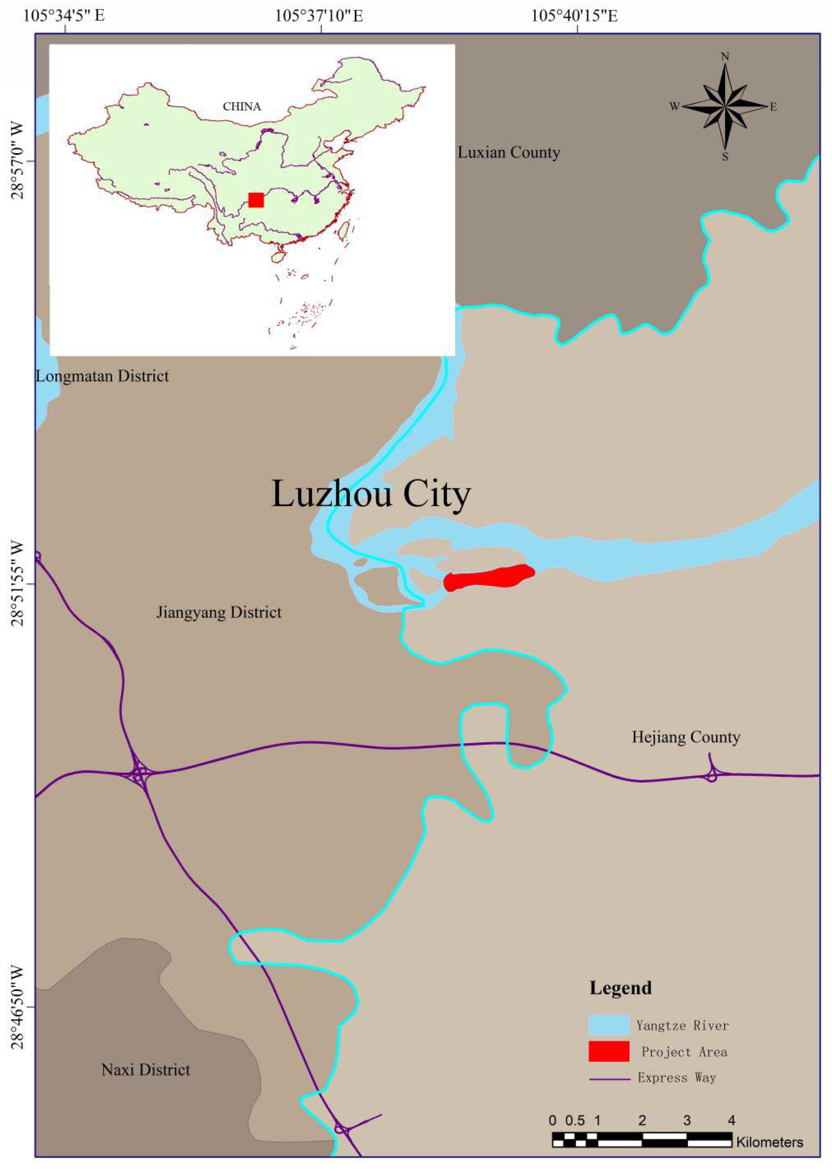
2.1. Study Area

The restoration project (coordinates: 28°51′45″ N, 105°39′33″ E) is located in Sichuan Province, in the core area of the rare and endemic fish nature reserve in the upper reaches of the Yangtze River (Figure 1). It is 190.0 km from the Xiangjiaba Dam, a giant hydropower station in the upstream reach of the project area. This area is one of the few river reaches that still has a lotic flow pattern in the upstream region of the Yangtze River since the cascade hydropower projects started running at full water capacity. Lotic conditions are of great significance for fish breeding, feeding, and even basic survival. However, Sand excavation and quarrying have flattened the landform of shorelines. Consequently, the topography has become so homogeneous that the water velocity has become too fast because of the lack of any blockage. This pattern represents a common situation in the upper reaches of the Yangtze River.

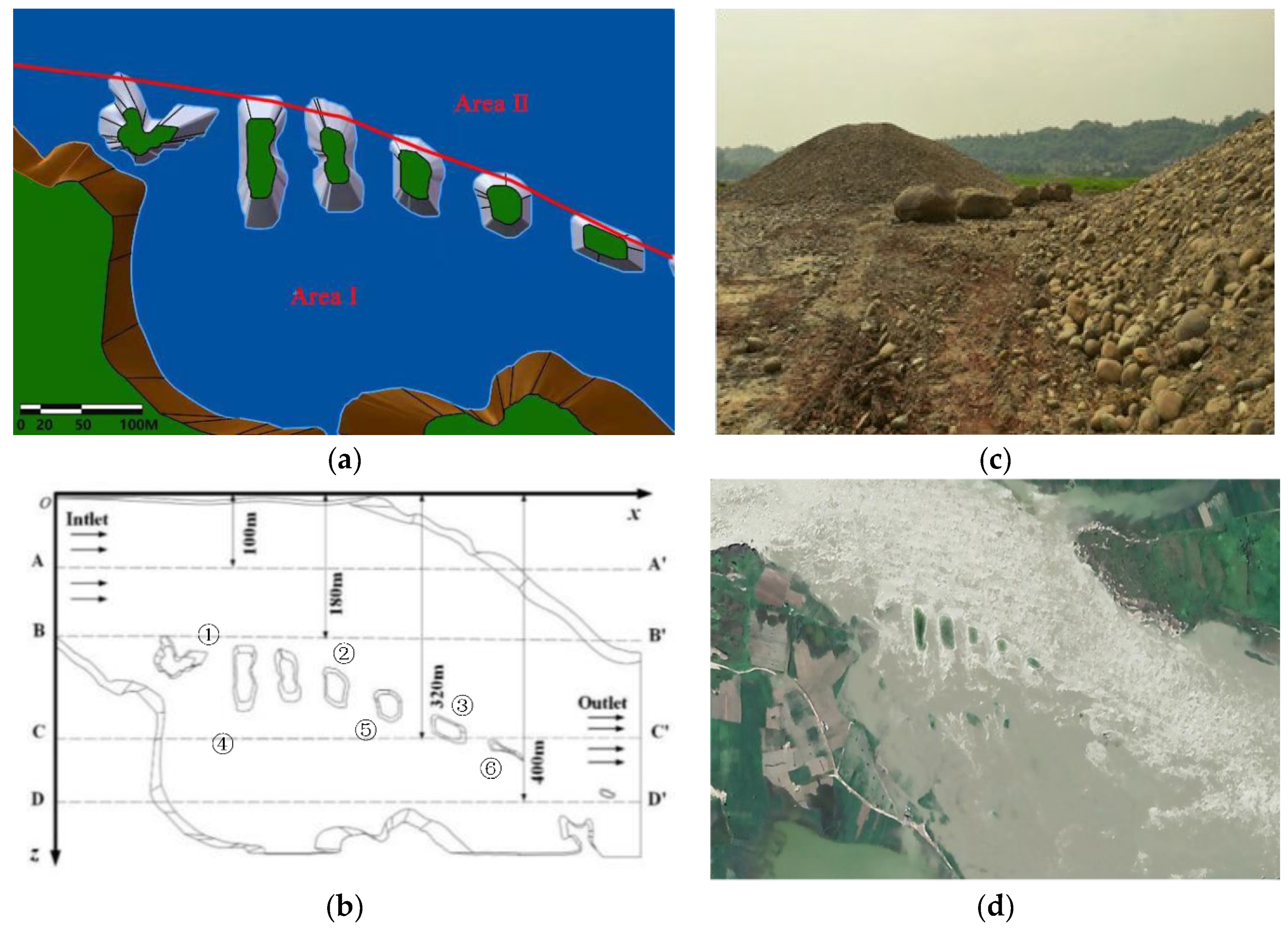
2.2. Restoration Project

The restoration project was located at a side channel. Because the main channel is protected by law for shipping purposes, it is a better option to implement river restoration in the side channel, which is less influenced by anthropogenic activity. One aim of all measures in this study is to enhance geomorphic heterogeneity. Therefore, we piled up gravel in the area to form six gravel bars of different shapes with a height of 6.0 m (Figure 2). The width of the ditches formed between the gravel bars was 16.0 m. The six gravel bars were arranged in a straight line in the longitudinal direction. The distance between the head gravel bar and the rear bar was 440.0 m. This measure attempted to support the riverine fauna by re-establishing natural flow and diverse water depth gradients. A variety of habitats would provide multifunctional spaces for different fish species or different life stages. The focus was placed on the fish community structure since this was the main goal of the restoration. The project was implemented and accomplished in August 2018.

2.3. Simulation of the Influence of Projects on Hydrological Conditions

2.3.1. Numerical Computational Model

To simulate and calculate the hydrodynamic characteristics of the fish habitat restoration project, a three-dimensional structure model of equal scale was established according to the gravel bar design prior to construction, and the flow field numerical computational model was then extracted. In this model, both the influence of the bank slope on the flow characteristics and the irregular slopes between the gravel bars were considered. The length and width of the computational model were 801.3 m and 486.8 m, respectively. The average depth of the normal water level was approximately 4.0 m, and the local water depth in the middle of the stream was approximately 5.0 m.

2.3.2. Study Design for Water Flow Pattern Change

To study the impact of constructed gravel bars on water flow and describe the geomorphic heterogeneity differences in respective areas, we defined the southern area of the gravel bars as Area I and the northern portion as Area II (Figure 2a).

2.3.3. Governing Equations and Turbulence Models

The fish habitats were three-dimensionally meshed using ANSYS MESH 18.2 software, and their simulations were conducted by ANSYS FLUENT 18.2. The liquid phase, gas phase and solid phase in water were regarded as incompressible and continuous mixed fluid phases, and the unsteady flow process satisfied the continuity equation and momentum conservation equation [35]:

$$\frac{\partial u}{\partial x}+\frac{\partial v}{\partial y}+\frac{\partial w}{\partial z}=0$$

(1)

$$\{\begin{array}{c}\frac{\partial u}{\partial t}+\left(u\frac{\partial u}{\partial x}+v\frac{\partial u}{\partial y}+w\frac{\partial u}{\partial z}\right)=F_x+\frac{u}{\rho }\left(\frac{{\partial }^{2}u}{\partial x^2}+\frac{{\partial }^{2}u}{\partial y^2}+\frac{{\partial }^{2}u}{\partial z^2}\right)\\ \frac{\partial v}{\partial t}+\left(u\frac{\partial v}{\partial x}+v\frac{\partial v}{\partial y}+w\frac{\partial v}{\partial z}\right)=F_y+\frac{u}{\rho }\left(\frac{{\partial }^{2}v}{\partial x^2}+\frac{{\partial }^{2}v}{\partial y^2}+\frac{{\partial }^{2}v}{\partial z^2}\right)\\ \frac{\partial w}{\partial t}+\left(u\frac{\partial w}{\partial x}+v\frac{\partial w}{\partial y}+w\frac{\partial w}{\partial z}\right)=F_z+\frac{u}{\rho }\left(\frac{{\partial }^{2}w}{\partial x^2}+\frac{{\partial }^{2}w}{\partial y^2}+\frac{{\partial }^{2}w}{\partial z^2}\right)\end{array}$$

(2)

where x, y, and z are rectangular coordinate components, ρ is the fluid density, μ is the viscosity coefficient of fluid, $F_x$, $F_y$, $F_z$ are the volume force components in a rectangular coordinate system, and u, v, and w are the velocity components in a rectangular coordinate system.

The RNG k-ε equation model was used in the turbulence model. The model can be used to describe complex flow problems such as shear flow with a large strain rate, swirl field and separation. The equations of turbulent kinetic energy k and turbulent dissipation rate ε were expressed as follows:

$$\{\begin{array}{c}\rho \frac{\partial \left(k\right)}{\partial t}+\rho \frac{\partial \left(k{u}_i\right)}{\partial x_i}=\frac{\partial }{\partial x_j}\left[\left(\mu +\frac{{\mu }_t}{{\sigma }_k}\right)\frac{\partial k}{\partial x_j}\right]+G_k+G_b-\rho \epsilon -Y_m+S_k \\ \rho \frac{\partial \left(\epsilon \right)}{\partial t}+\rho \frac{\partial \left(\epsilon u_i\right)}{\partial x_i}=\frac{\partial }{\partial x_j}\left[\left(\mu +\frac{{\mu }_t}{{\sigma }_{\epsilon }}\right)\frac{\partial \epsilon }{\partial x_j}\right]+C_1\frac{\epsilon }{k}\left(G_k+C_u{G}_b\right)-C_2\rho \frac{{\epsilon }^2}{k}+S_{\epsilon } \end{array}$$

(3)

$G_k$ represents the kinetic energy generated by the change in fluid velocity:

$$G_k={\mu }_t\left(\frac{\partial u_i}{\partial x_j}+\frac{\partial u_j}{\partial x_i}\right)\frac{\partial u_i}{\partial x_j}$$

(4)

${\mu }_t$ represents the turbulent viscosity coefficient:

$${\mu }_t=\rho C_{\mu }\frac{k^2}{\epsilon }$$

(5)

where ${\sigma }_k$ and ${\sigma }_{\epsilon }$ are related to the turbulent kinetic energy k and turbulent dissipation rate ε. $S_k$ and $S_{\epsilon }$ are the calculation terms estimated from existing data according to the actual situation. $G_b$ represents the turbulent kinetic energy generated by external influence. $Y_m$ is the term in a fluid that provides energy. The turbulent viscosity ratio ${\mu }_t/\mu$ is directly proportional to the turbulent Reynolds number and is generally taken as 1~10 in hydraulics. The empirical coefficients are as follows: ${\sigma }_k=0.7179$, $C_1=1.42$, $C_2=1.68$, and $C_{\mu }=0.09$ [35].

2.4. Numerical Grid Parameters

To study the hydrodynamic characteristics of different areas, the oxz plane was used to establish the coordinate system, and the x direction was the flow direction. Section AA’ was parallel to the x axis and perpendicular to the z axis, with 0A = 100 m. Sections BB’, CC’ and DD’ were parallel to section AA’. The distance between parallel lines is shown in Figure 2. Detailed grid refinement was conducted for gravel bars with different shapes and irregular river banks where flow changed violently. A grid interface was adopted at the grid junction, and a boundary layer grid was added in the area close to the slope surface. The unstructured grid was divided and then verified for grid independence. The total number of grids was determined to be approximately 20 million. The minimum grid size was 5 mm and the maximum grid size was 100 mm.

In the calculation model, the bank, bottom and gravel bars were set as the boundary conditions without sliding, and the river roughness n was set as 0.03. The water surface was defined as the axisymmetric boundary condition, and the entrance of the flow field was defined as the inlet velocity boundary condition. The initial velocity was determined according to the average value of the river reach recorded at different times, and the values were v₀ = 2 m/s, v₀ = 3 m/s, v₀ = 4 m/s, and v₀ = 5 m/s. The flow field outlet was defined as the pressure outlet boundary condition. The river’s water density was 1052 kg/m³, the kinematic viscosity coefficient was 1.0565 × 10⁶ m²/s, and the operating pressure was 101325 Pa. The SIMPLEC (Semi-Implicit Method for Pressure Linked Equations) algorithm based on pressure coupling was adopted. The second-order upwind scheme was used for both turbulent kinetic energy and turbulent dissipation rate.

2.5. Hydromorphological Survey and Model Validation

Water velocities were measured with a FlowQuest2000 ADCP (acoustic Doppler current profiler) mounted to the side board of a moving fishing ship. ADCP surveys were conducted in August 2018. Following the surveys, ADCP data were processed using the software package Discharge to project replicates of the transects to a mean transect line [36]. The water depth, velocity and flow direction of different depth layers on each vertical line were extracted. Then, the transverse and longitudinal velocities were calculated to generate the flow pattern diagram. The numerical model was validated by comparing the measured ADCP data with the depth-averaged velocity in the section of Area I.

2.6. Fish Survey

The evaluation of fish community structure variation followed “before–after” experiment design [37]. Six sample points at 200.0 m intervals located on both sides of the gravel bars were collected (Figure 2b). To compare the changes in fish species number, abundance, and biomass before and after the implementation of the project, samples were obtained in February, April and June of 2018 and February, April and June of 2019. Four gill nets and four ground cages were placed at each sampling point. The gill nets were 100.0 m long and 2.0 m high with mesh sizes of 2.0, 4.0, 6.0 and 8.0 cm. The placement direction was vertical to the water flow direction, and the placement time was 12 h. Ground cages were 20.0 m long, 32.0 cm wide and 24.0 cm high, with the 0.5-cm-dimension of the mesh placed parallel to the water flow. The ground cages were also placed for approximately 12 h. To ensure the effectiveness of fish sampling, we selected lower flow conditions below 0.5 m/s during each sampling time.

Data on the species number, biomass, abundance and ecological types of captured fish were collected. The species were identified based on morphological traits [38,39]. The abundance data were used to record the total catch of each species at each point, and the biomass was determined using an electronic scale with an accuracy of 0.1 g to obtain the fresh weight of each fish. The classification of ecological types is based on Wang et al. [40].

2.7. Statistical Analysis

2.7.1. Fish Composition Analysis

Fish species number, abundance and biomass were summed across the six sampling points and all months sampled to compare the fish resource variation before and after the project. One-way ANOVA was conducted between the total species number, abundance and biomass before and after the implementation of the project. p < 0.05 indicates a significant difference and p < 0.01 indicates an extremely significant difference. The relative importance index (IRI) proposed by Pinkas was used to identify the significance of each species in the fish community, and the species with IRI > 1000 were considered dominant species while the species with 100 ≤ IRI < 1000 were defined as common species. The IRI was calculated as follow [41]:

IRI = F(N′ + W′) × 10,000

where N′ is the proportion of a certain species to the total, W′ is the proportion of the mass of a certain species to the total, F is the proportion of the number of points of a certain species to the total number of points investigated.

2.7.2. Fish Ecological Behavior Trait Analysis

The collected fish were divided into five categories according to their ecological habits. The five categories were further divided into 16 subclasses as follows: migration types included freshwater settlement type and river-lake migration type; trophic guild included planktonic, carnivorous, omnivorous and phytophagous; spawning type included demersal egg, pelagic egg, shellfish laying egg, drifting egg and adhesive egg; flow preference included lotic type and lentic type; water layer explored included pelagic fishes, middle-lower fishes and demersal fishes [42]. One-way ANOVA was conducted between the data collected before and after the implementation of the project. p < 0.05 indicates significant difference and p < 0.01 indicates extremely significant difference between each ecological behavior trait.

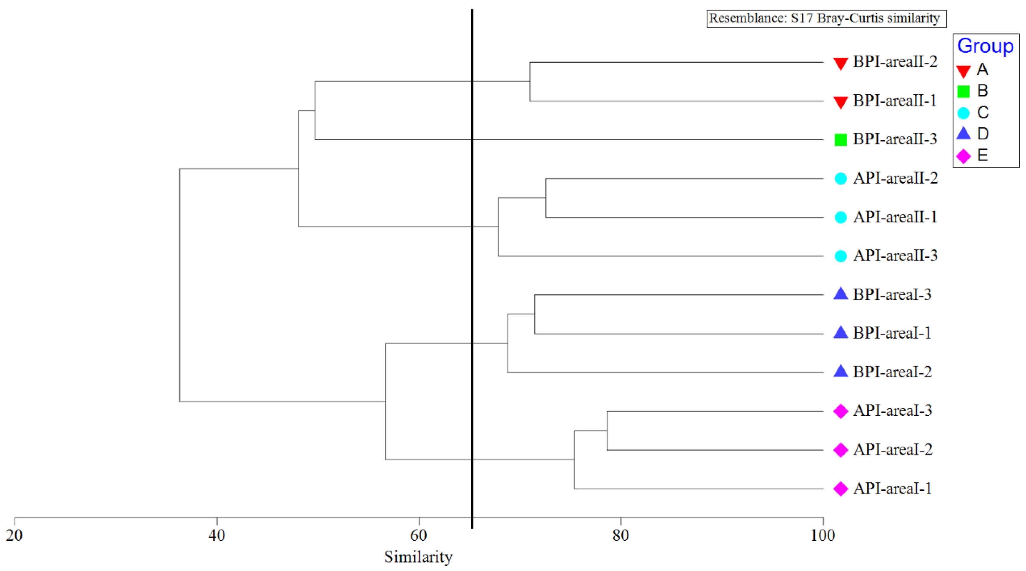
2.7.3. Cluster Analysis of Fish Community Structure

Cluster analysis was conducted on the fish abundance in 12 quadrats composed of various sampling points before and after the implementation of the project. The six sampling points were marked as BPI-area I-1, BPI-area I-2, BPI-area I-3, BPI-area II-1, BPI-area II-2, BPI-area II-3 before the project implementation and API-area I-1, API-area I-2, API-area I-3, API-area II-1, API-area II-2, API-area II-3 after the project. First, the reassembly analysis was carried out after the data table was established in PRIMER 7.0 software developed by Clarke and Gorley [43]. Through the Bray Curtis dissimilarity method [44], the similarity matrix between quadrats was established and a cluster diagram was drawn. Twelve quadrats were classified into groups and it was determined whether the division of groups was credible using similarity test analysis. A significance level of the sample statistic (Sig.) <0.05 indicated that it was credible [45]. In addition, nonmetric multidimensional scaling (NMDS) was used to analyse the similarity matrix between quadrats, and the stress coefficient was used to measure the effect of the NMDS two-dimensional dot matrix distribution map. It is generally considered that the results are very representative when stress < 0.05 and basically credible when 0.05 ≤ stress < 0.10 [46]. Similarity percentage (SIMPER) was used to measure the species composition difference between groups, and to explore the main species causing the difference between groups and their contribution to the dissimilarities [47]. Only species with a cumulative contribution of 70% for dissimilarities are presented.

3. Results

3.1. Analysis of Flow Characteristics

3.1.1. Hydromorphological Condition Verification

The field survey results after the implementation of the project showed that the velocity at Area I had a water flow range of 0.29–2.45 m/s, with an average of 1.62 m/s (Figure 3a). Because the flow velocity at Area II was too fast for the survey ship to enter, for safety reasons, we measured the surface velocity near the river bank of Area II with a rotameter instead, and the value was 4.30 m/s. This flow condition was similar to that of the inflow velocity set as 4.0 m/s. Therefore, the simulation average flow velocity at v₀ = 4.0 m/s of Area I was compared with the ADCP measured result to test the accuracy. It was found that the ADCP average velocity was an approximation of the simulation value (1.60 m/s), with a minor difference of 0.02 m/s (see Supplementary Figure S4c for simulation velocity distributions of the flow field at inflow 4.0 m/s). The bulk flow speed was matched between the field measurements and the numerical simulation.

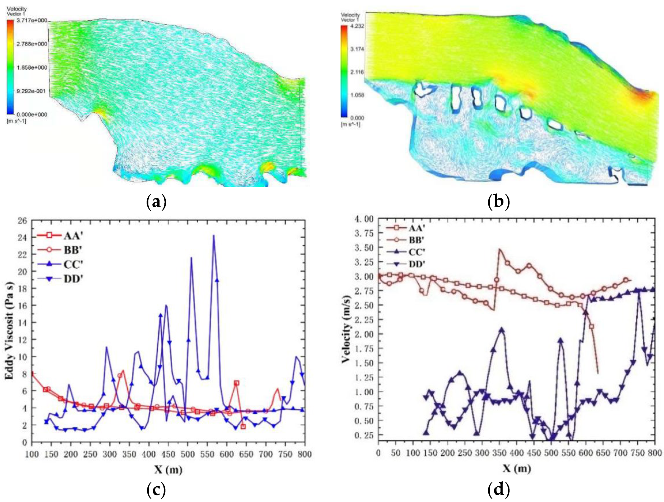
3.1.2. Flow Field Simulation

Modelling the flow showed that there was an obvious water diversion phenomenon when the water flowed through the gravel bars, with the part entering Area I with a smaller velocity than in Area II (Figure 3b). It is noteworthy that the nephogram before implementing the program indicated a more homogeneous water flow (Figure 4a). Due to the water blocking effect of the gravel bars, the flow direction in Area I changed diversely. By comparison, the flow in Area II was relatively fast with no obvious change in the flow direction. A small eddy current structure and wake flow were formed between gravel bars. Five large vortices were formed in Area I (Figure 4b). Moreover, it was seen that the shapes of the vortex structure basically did not vary with the changes in the in-flow velocity. The upwelling in the anticlockwise vortex was more obvious with a slightly higher velocity than that in the clockwise vortices.

3.1.3. Turbulence Characteristics Simulation

It was found that the turbulent viscosity of Area I changed more greatly at different inflow velocities than that at Area II. The average viscosity increased to 9.1 Pa s at Area I compared with 4.6 Pa s at Area II as the inflow velocity was set at v₀ = 3.0 m/s (Figure 4c). Affected by the gravel bars, backflow and circulation were recreated in Area I, where the flow field was more complex and disordered.

3.1.4. Velocity Distribution Simulation on Longitudinal Cross-Sections

Flow modelling showed that Area II presented a less variable and higher flow velocity than Area I. The average velocities were 1.6, 2.4, 3.2 and 4.5 m/s at inflow velocities of 2.0, 3.0, 4.0 and 5.0 m/s, respectively. The average velocities at Area I were 0.7, 1.2, 1.6 and 1.8 m/s at inflow velocities of 2.0, 3.0, 4.0 and 5.0 m/s, respectively (Figure 4d).

3.2. Fish Resources

3.2.1. Fish Composition

The fish species collected before and after the implementation of the project are provided in the Supplementary Material (see Supplementary Table S1).

It was found that the number of fish species was 40, the catch abundance was 670 and the catch biomass was 19977.3 g before the implementation of the project. After the project, the number of fish species was 49, the abundance was 1327 and the biomass was 32501.8 g. One-way ANOVA results showed that there were significant differences in the number of species (F = 5.066, p < 0.05) and the catch abundance (F = 4.856, p < 0.05) before and after the project (Figure 5).

After the implementation of the project, nine more fish species were collected. The number of rare and endemic fish species in the upper reaches of the Yangtze River increased from 4 to 9. As a result, the proportion of these protected species among all the fish collected increased by 8.37%. The analysis of the changes in fish species composition indicated that few fish species were collected only before or after the implementation of the project (

Table 1. Fish species caught only before the implementation of the project or after the project. “☐” indicates endemic fish; “▲” indicates rare fish. “BPI” is the abbreviation of “before the implementation”; “API” is the abbreviation of “after project implementation”. Endemic or rare species were classified according to Cao [10].

Species	Rare and Endemic Fish	Capture Period	Abundance/Ind.	Biomass/g
Monopterus albus (Zuiew)		BPI	1	30.20
Acrossocheilus monticola (Günther)	☐	BPI	2	35.80
Hemiculterella sauvagei	☐	API	48	412.80
Ancherythroculter kurematsui (Kimura)	☐	API	1	33.00
Xenocypris davidi (Bleeker)		API	1	76.60
Culter mongolicus (Basilewsky)		API	9	2095.20
Rhodeus sinensis (Kaer)		API	7	130.10
Pseudobrama simoni (Bleeker)		API	3	106.80
Procypris rabaudi (Tchang)	☐	API	1	82.70
Squalidus argentatus		API	17	207.70
Xenocypris yunnanensis (Nichols)	☐	API	1	243.90
Acipenser dabryarus (Dumeril)	▲	API	1	54.80
Rhinogobio ventralis (Savage et Dabry)	☐	API	1	112.20

). For rare and endemic fish species, Acrossocheilus monticolus was not caught, but six additional species were collected after the project.

The calculation results of the relative importance index showed that there were 11 dominant and common fish species before the implementation of the project with a corresponding total abundance of 577 and total biomass of 15,586.0 g. After the project, the dominant and common fish increased to 15 species, with a total abundance of 1156 and a total biomass of 27,148.6 g, respectively (

Table 2. Dominant and common species before and after project implementation, and their corresponding abundance and biomass. Species with IRI > 1000 were considered dominant species while species with 100 ≤ IRI < 1000 were defined as common species. “BPI” is the abbreviation of “before the implementation”; “API” is the abbreviation of “after project implementation”.

Species	Abundance/ Ind.		Biomass/g		IRI
	BPI	API	BPI	API	BPI	API
Carassius auratus (Linnaeus)	135	224	3145	5105	2393	2353
Saurogobio dabryi (Bleeker)	69	230	1332	3329	848	1991
Hemiculter leucisculus (Basilewsky)	93	166	1742	2673	1632	1613
Cyprinus carpio (Linnaeus)	31	34	4029	4217	1102	691
Trilophysa bleekeri (Sauvage et Dabry)	77	107	346	369	808	613
Pseudolaubuca engraulis (Nichols)	34	59	825	1334	307	380
Culter ilishaeformis (Bleeker)	3	74	176	1770	\	367
Culter mongolicus (Basilewsky)	\	9	\	2095	\	237
Abbottina rivularis (Basilewsky)	17	41	129	208	124	187
Rhodeus sinensis (Kaer)	8	29	54	161	\	179
Ctenopharyngodon idellus (Cuvier et Valenciennes)	2	9	1573	3082	\	169
Hemiculterella sauvagei	\	48	\	413	\	163
Hemibarbus maculatus (Bleeker)	13	43	262	297	\	139
Zacco platypus (Temminck et Schlegel)	12	15	898	1144	175	129
PelteobagrusVachelli (Richardson)	6	26	125	379	\	122
Rhinogobius giurinus (Rutter)	39	21	196	78	302	\
Sinibrama taeniatus (Nichols)	19	13	248	263	136	\
Leiocassis crassilabris (Günther)	19	8	507	241	119	\

).

3.2.2. Fish Ecological Behavior Trait

The fish were divided into five categories according to their ecological habits: migration type, trophic guild, spawning type, flow preference and water layer explored, which can be divided into 16 subcategories (Figure 6). Among them, the species numbers of 10 subcategories increased after the implementation of the project. The differences in freshwater settlement type (F = 4.227, p < 0.05), river–lake migration type (F = 6.359, p < 0.05), demersal egg (F = 4.815, p < 0.05), omnivorous (F = 4.447, p < 0.05) and pelagic fishes (F = 7.198, p < 0.05) were significant, while those of shellfish laying eggs (F = 11.769, p < 0.01) and planktonic (F = 9.842, p < 0.01) were extremely significant before and after the project. For fish abundance, all 16 subcategories increased after the implementation of the project. There were significant differences in freshwater settlement type (F = 4.007, p < 0.05), demersal egg (F = 5.583, p < 0.05), drifting egg (F = 4.783, p < 0.05), omnivorous (F = 4.423, p < 0.05), lentic type (F = 4.421, p < 0.05), pelagic fish (F = 6.117, p < 0.05), and middle–lower fish (F = 4.422, p < 0.05) and extremely significant differences in river–lake migration type (F = 9.140, p < 0.01), shellfish laying eggs (F = 7.611, p < 0.01), and planktonic (F = 11.703, p < 0.01). For the biomass, fifteen subcategories increased after the implementation of the project. There were significant differences in demersal egg (F = 4.231, p < 0.05), shellfish laying eggs (F = 5.514, p < 0.01) and extremely significant differences in planktonic (F = 7.862, p < 0.01).

3.2.3. Analysis of Differences among Fish Communities

The cluster analysis results showed that the fish community could be divided into five groups (groups A~ E) at the 65% similarity level (Figure 7). NMDS analysis indicated that BPI-area II-1 and BPI-area II-2 were divided into group A; BPI-area II-3 was divided into group B; API-area II-1, API-area II-2, and API-area II-3 were divided into group C; BPI-area I-1, BPI-area I-2, and BPI-area I-3 were divided into group D and API-area I-1, API-area I-2, and API-area I-3 were divided into group E. The results of the similarity single factor test showed that the group division was credible with Sig. 0.1% (<0.05). The stress value shows that the NMDS diagram was basically credible.

The results of SIMPER analysis (

Table 3. SIMPER analysis of five groups of fish communities. Only species which sum > 70% contribution to dissimilarities are presented. “\” indicates no data.

Species	A Group and B Group		A Group and C Group		D Group and E Group
	Av.Diss	Contrib%	Av.Diss	Contrib%	Av.Diss	Contrib%
Trilophysa bleekeri (Sauvage et Dabry)	7.5	14.9	3.7	7.0	2.1	4.7
Hemiculter leucisculus (Basilewsky)	7.1	14.2	\	\	6.1	14.1
Pseudolaubuca engraulis (Nichols)	4.7	9.4	\	\	1.7	4.0
Carassius auratus (Linnaeus)	4.7	9.4	8.0	15.2	4.0	9.2
Liobagrus marginatus (Günther)	3.7	7.4	2.5	4.7	\	\
Abbottina rivularis (Basilewsky)	3.4	6.8	\	\	1.7	3.9
Rhinogobius giurinus (Rutter)	2.7	5.4	\	\	1.5	3.5
Sinibrama taeniatus (Nichols)	2.6	5.2	2.5	4.7	\	\
Saurogobio dabryi (Bleeker)	\	\	10.1	19.3	7.3	16.9
Hemiculterella sauvagei	\	\	8.5	16.2	\	\
Leiocassis crassilabris (Günther)	\	\	2.5	4.7	\	\
Culter ilishaeformis (Bleeker)	\	\	\	\	4.5	10.3
Hemibarbus maculates (Bleeker)	\	\	\	\	2.1	4.9
Cumulative contribution rate		72.8		70.2		71.5

) showed that the dissimilarity rate between group A and group B was 50.32%. The contribution rate of 8 fish species to the cumulative difference between groups was 72.79%, including Trilophysa bleekeri (the average dissimilarity between groups was 7.47, and the contribution rate was 14.85%), Hemiculter leucisculus (the dissimilarity between groups was 7.16, and the contribution rate was 14.22%) and so on. The dissimilarity rate between group A and group C was 52.22%. The contribution rate of seven species to the cumulative difference between groups was 70.21%, including Saurogobio dabryi (the average dissimilarity between groups was 10.07 and the contribution rate was 19.28%), Hemiculterella sauvagei (the average dissimilarity between groups was 8.45 and the contribution rate was 16.18%) and so on. The dissimilarity rate between group D and group E was 43.33%. The cumulative contribution rate of nine species of fish to the difference between groups was 71.47%, including Saurogobio dabryi (the average dissimilarity between groups was 7.33 and the contribution rate was 16.92%), Hemiculter leucisculus (the average dissimilarity between groups was 6.12 and the contribution rate was 14.13%) and so on.

4. Discussion

4.1. Projected Effect on Hydromorphology

More recently, river restoration projects have been well established at an increasing rate in many regions to recreate habitats by improving substratum quality, especially for spawning and recruiting [48,49,50,51]. The European Union reacted to the predicted loss of biodiversity and resulting decrease in human well-being by proclaiming the Water Framework Directive (WFD) in 2000 [52]. Within this framework, the effectiveness of all river restoration techniques was comprehensively researched and detected [53,54,55]. To increase the possibility of successful restoration of fish habitats in the Yangtze River, we considered all major restoration efforts in successful cases. Finally, we opted for habitat restructuring to stabilize river morphology, which has proven to be a powerful tool to combat hydromorphological degradation [56,57,58]. A series of gravel bars functioning as water current regulation facilities were constructed in a side channel on the Yangtze River. The results of the numerical computational simulation showed that compared with Area II, the construction of the gravel bars effectively changed the flow velocity in Area I. Under the condition of an inflow velocity of 2.0–5.0 m/s, the average velocity of Area I was approximately 0.7–1.8 m/s. The field survey using ADCP results also verified the accuracy of the computer simulation data. This approach was very suitable for the survival of protected fish in the reach. Other studies have shown that the survival of river fish is highly dependent on hydrodynamic and morphological conditions, and the hydraulic state of these two aspects is determined by the topography of the habitat [57,59]. In this study, the gravel bars built based on the theory of habitat geomorphology diversity [60] improved the hydrodynamic environment of fish survival. Eddy structures, turbulent flows and upwelling were formed in the restoration project. Because vortices have field characteristics and absorb material, this low-speed turbulent vortex structure was helpful for fish assemblages. Recreated backflow and circulation made the flow field more complex. These are important hydraulic conditions for improving fish diversity. The erosive forces potentially caused by the vorticity increase are one of our key considerations. The stability of the gravel bars is being monitored. So far, all the gravel bars have remained stable because the gravels we deployed were relatively large (10~60 cm). The expected half-life of the gravel bars is about 15 years. Additionally, the project was implemented in a side channel which discharged into the trunk stream from downstream. So, the sharp contrast in flow between the two areas is less likely to influence the biological connectivity downstream.

4.2. Projected Effect on Fish Species

Our results showed that the main aim of the restoration measures to physically increase habitat diversity was met, and more natural river structures were created. This led to a greater variety of habitats and higher microhabitat diversity, increasing the availability of good potential spawning and nursing habitats [61]. Fish species diversity increases with the diversity of hydraulic morphology, which is determined by the topography and geomorphology of the habitat [62,63,64,65,66,67,68]. Therefore, the foundations for a positive impact on the fish fauna were laid. After the implementation of the project, nine additional kinds of fish were collected, and six species of them were target species of protected fish in the upper reaches of the Yangtze River. Among them, Yangtze sturgeon (Acipenser dabryanus) is a national first-class protected wild animal [10]. The results showed that the response of fish assemblages to river restoration was positive, especially for rare and endemic fish in the upper reaches of the Yangtze River. In comparison, the catch biomass was 1.63-fold higher than that before the implementation of habitat restoration, indicating that habitat restoration could increase fish resources by providing a variety of habitats supporting different ecological types of fish.

The results showed that our hypothesis that river restoration will lead to an increase in fish abundance was supported. Most of the species of conservation concern in the reach are small-bodied rheophilic fishes [66]. Compared with stagnophilic species, rheophilic fishes are much more dependent on the river flow regime and more sensitive to hydraulic condition changes [68]. Restoration projects created more stable and suitable water current velocities by increasing physical habitat structure heterogeneity [68,69]. It was found that the turbulent viscosity changed greatly as the project was implemented in this study. Turbulent viscosity refers to the strong vortex diffusion and cascade dispersion caused by random fluctuation when the fluid flow is in the turbulent state. It is an important parameter used to characterize the turbulence. Its mechanism is that the vortex drives the fluid particles to move randomly, resulting in a strong momentum transfer rate, which makes the apparent viscosity far greater than the viscosity at the molecular level. Backwaters recreated by gravel bar reconfiguration are essential environmental factors that are required for the survival of rheophilic fish. If the flow is too slow, fish eggs will sink to the bottom and die. If the flow is too fast, larval and juvenile fish will be flushed out of the habitat [70,71,72,73]. Therefore, adaptations in this research attempted to modify flow patterns to more natural conditions and could provide nursery areas for larval and juvenile fish and shelters for small-bodied fish such as Hemiculterella sauvagei [74,75,76,77,78,79]. More heterogeneous habitats with diverse, near-natural flow velocities and water depth gradients indicated strong fish assemblages in the Yangtze River.

4.3. Summary and Future Research Recommendations

The results of our research suggest that river restoration significantly enhanced fish habitat conditions in the Yangtze River. Moreover, a positive effect of a restoration project was found on fish diversity and abundance. The adopted measure succeeded in re-establishing key abiotic factors befitting to fish species targeting. Fish habitat use is highly variable between years [79]. Furthermore, it takes several years for fish habitat restoration to reach an ecological balance and self-sustainability (generally 5 to 8 years). Therefore, long-term monitoring of fish community status variation should be included to fully understand restoration effects. Finally, we strongly suggest that many more other restoration measures should be conducted in the Yangtze River to protect fish following the different ecological guides and life strategies. This diverse approach is crucial for identifying the most feasible measures to reach the objective of a “good ecological potential” in the Yangtze River.

References

1. Mccluney, K.E.; Poff, L.R.; Palmer, M.A.; Thorp, J.H.; Poole, G.C.; Williams, B.S.; Williams, M.R.; Baron, J.S. Riverine macrosystems ecology: Sensitivity, resistance, and resilience of whole river basins with human alterations. Front. Ecol. Environ. 2014, 12, 48–58. [Google Scholar] [CrossRef]
2. Palmer, M.A.; Richardson, D.C. Provisioning Services: Afocus on Fresh Water; Princeton University Press: Princeton, NJ, USA, 2009. [Google Scholar]
3. Strayer, D.L.; Dudgeon, D. Freshwater biodiversity conservation: Recent progress and future challenges. J. N. Am. Benthol. Soc. 2010, 29, 344–358. [Google Scholar] [CrossRef] [Green Version]
4. Winemiller, K.O.; McIntyre, P.B.; Castello, L.; Fluet-Chouinard, E.; Saenz, L. Balancing hydropower and biodiversity in the Amazon, Congo, and Mekong. Science 2016, 351, 128–129. [Google Scholar] [CrossRef] [PubMed] [Green Version]
5. Carlisle, D.M.; Falcone, J.; Wolock, D.M.; Meador, M.R.; Norrjs, R.H. Predicting the natural flow regime: Models for assessing hydrological alteration in streams. River Res. Appl. 2010, 26, 118–136. [Google Scholar] [CrossRef]
6. Poff, L.R.; Olden, J.D.; Merritt, D.M.; Pepin, D.M. Homogenization of regional river dynamics by dams and global biodiversity implications. Proc. Natl. Acad. Sci. USA 2007, 104, 5732–5737. [Google Scholar] [CrossRef] [PubMed] [Green Version]
7. Bunn, S.E.; Arthington, A.H. Basic Principles and Ecological Consequences of Altered Flow Regimes for Aquatic Biodiversity. Environ. Manag. 2002, 30, 492–507. [Google Scholar] [CrossRef] [PubMed] [Green Version]
8. Lehner, B.; Liermann, C.R.; Revenga, C.; Vorosmarty, C.; Fekete, B.; Crouzet, P.; Döll, P.; Endejan, M.; Frenken, K.; Magome, J.; et al. High-resolution mapping of the world’s reservoirs and dams for sustainable river-flow management. Front. Ecol. Environ. 2011, 9, 494–502. [Google Scholar] [CrossRef] [Green Version]
9. Power, M.E.; Dietrich, W.E.; Finlay, J.C. Dams and downstream aquatic biodiversity: Potential food web consequences of hydrologic and geomorphic change. Environ. Manag. 1996, 20, 887–895. [Google Scholar] [CrossRef]
10. Cao, W.X. Several problems on the protection of fish resources in the Yangtze River Basin. Resour. Environ. Yangtze Basin 2008, 17, 163–164. [Google Scholar]
11. Duan, X.B.; Tian, H.W.; Gao, T.H.; Liu, S.P.; Wang, K.; Chen, D.Q. Resources status of ichthyoplankton in the Upperyangtze River before the storage of JinSha River first stage project. Resour. Environ. Yangtze Basin 2015, 24, 1358–1366. [Google Scholar]
12. Fu, C. Freshwater fish biodiversity in the Yangtze River basin of China patterns, threats and conservation. Biodivers Conserv. 2003, 12, 1649–1685. [Google Scholar] [CrossRef]
13. Gao, T.H.; Tian, H.W.; Ye, C.; Duan, X.B. Diversity and composition of fish in the mainstream of national nature reserve of rare and endemic fish in the upper Yangtze River. Freshw. Fish 2013, 43, 36–42. [Google Scholar]
14. Zhao, W.H.; Cao, H.Q.; Huang, Z.; Wang, Z.H. Assessment of physical integrity of National Nature Reserve for rare and endemic fishes in upstream Yangtze River before and after xiangjiaba dam impoundment. J. Yangtze River Sci. Res. Inst. 2015, 32, 76–80. [Google Scholar]
15. Palmer, M.A.; Hondula, K.L.; Koch, B.J. Ecological Restoration of Streams and Rivers: Shifting Strategies and Shifting Goals. Annu. Rev. Ecol. Evol. Syst. 2014, 45, 247–269. [Google Scholar] [CrossRef] [Green Version]
16. Nilsson, C.; Aradottir, A.L.; Hagen, D.; Halldórsson, G.; Høegh, K.; Mitchell, R.J.; Raulund-Rasmussen, K.; Svavarsdóttir, K.; Tolvanen, A.; Wilson, S.D. Evaluating the process of ecological restoration. Ecol. Soc. 2016, 21, 41. [Google Scholar] [CrossRef] [Green Version]
17. Tockner, K.; Uehlinger, U.; Robinson, C.T. Rivers of Europe; Academic Press: Berlin/Heidelberg, Germany, 2009. [Google Scholar]
18. Boedeltje, G.; Smolders, A.J.P.; Roelofs, J.G.M.; Van Groenendael, J.M. Constructed shallow zones along navigation canals: Vegetation establishment and change in relation to environmental characteristics. Aquat. Conserv. Mar. Freshw. Ecosyst. 2001, 11, 453–471. [Google Scholar] [CrossRef]
19. Brookes, A. The distribution and management of channelized streams in Denmark. Regul. Rivers Res. Manag. 1987, 1, 3–16. [Google Scholar] [CrossRef]
20. Jähnig, S.C.; Lorenz, A.W. Substrate-specific macroinvertebrate diversity patterns following stream restoration. Aquat. Sci. 2008, 70, 292–303. [Google Scholar] [CrossRef]
21. Jähnig, S.C.; Brabec, K.; Buffagni, A.; Erba, S.; Lorenz, A.W.; Ofenböck, T.; Verdonschot, P.F.M.; Hering, D. A comparative analysis of restoration measures andtheir effects on hydromorphology and benthic invertebrates in 26 central andsouthern European rivers. J. Appl. Ecol. 2010, 47, 671–680. [Google Scholar] [CrossRef]
22. Sundermann, A.; Antons, C.; Cron, N.; Lorenz, A.W.; Hering, D.; Haase, P. Hydromorphological restoration of running waters: Effects on benthic invertebrate assemblages. Freshw. Biol. 2011, 56, 1689–1702. [Google Scholar] [CrossRef]
23. Vogt, T.; Hoehn, E.; Schneider, P.; Freund, A.; Schirmer, M.; Cirpka, O.A. Fluctuations of electrical conductivity as a natural tracer for bank filtration in a losing stream. Adv. Water Resour. 2010, 33, 1296–1308. [Google Scholar] [CrossRef]
24. Mueller, M.; Pander, J.; Geist, J. The ecological value of stream restoration measures: An evaluation on ecosystem and target species scales. Ecol. Eng. 2014, 62, 129–139. [Google Scholar] [CrossRef]
25. Pander, J.; Mueller, M.; Geist, J. A comparison of four stream substratum restoration techniques concerning interstitial conditions and downstream effects. River Res. Appl. 2015, 31, 239–255. [Google Scholar] [CrossRef]
26. Lu, W.; Font, R.A.; Cheng, S.; Wang, J.; Kollmann, J. Assessing the context and ecological effects of river restoration—A meta-analysis. Ecol. Eng. 2019, 136, 30–37. [Google Scholar] [CrossRef]
27. Ebel, G. Untersuchungen zur Stabilisierung von Barbenpopulationen-Dargestellt am Beispiel Eines Mitteldeutschen Fließgewässers; Eigenverlag: Halle, Germany, 2002. [Google Scholar]
28. Hauer, C.; Unfer, G.; Schmutz, S.; Habersack, H. The importance of morphody-namic processes at riffles used as spawning grounds during the incubation timeof nase (Chondrostoma nasus). Hydrobiologia 2007, 579, 15–27. [Google Scholar] [CrossRef]
29. Hauer, C.; Unfer, G.; Schmutz, S.; Habersack, H. Morphodynamic effects onthe habitat of juvenile cyprinids (Chondrostoma nasus) in a restored Austrianlowland river. Environ. Manag. 2008, 42, 279–296. [Google Scholar] [CrossRef]
30. Kondolf, G.M. Assessing Salmonid Spawning Gravel Quality. Trans. Am. Fish. Soc. 2000, 129, 262–281. [Google Scholar] [CrossRef]
31. Pulg, U.; Barlaup, B.T.; Sternecker, K.; Trepl, L.; Unfer, G. Restoration of spawning habitats of brown trout (Salmo trutta) in a regulated chalk stream. River Res. Appl. 2013, 29, 172–182. [Google Scholar] [CrossRef]
32. Schmutz, S.; Kremser, H.; Melcher, A.; Jungwirth, M.; Muhar, S.; Waidbacher, H.; Zauner, G. Ecological effects of rehabilitation measures at the Austrian Danube: A meta-analysis of fish assemblages. Hydrobiologia 2014, 729, 49–60. [Google Scholar] [CrossRef]
33. Lorenz, A.W.; Stoll, S.; Sundermann, A.; Haase, P. Do adult and YOY fish benefit from river restoration measures? Ecol. Eng. 2013, 61, 174–181. [Google Scholar] [CrossRef]
34. Kottelat, M.; Freyhof, J. Handbook of European Freshwater Fishes; Kottelat, Cornol & Freyhof: Berlin, Germany, 2007. [Google Scholar]
35. Zhou, L.; Wang, Z. Numerical simulation of cavitation around a hydrofoil and evaluation of a RNG κ-ε model. J. Fluids Eng. Trans. ASME 2008, 130, 011302. [Google Scholar] [CrossRef]
36. Fischer, J.L.; Filip, G.P.; Alford, L.K.; Roseman, E.F.; Vaccaro, L. Supporting aquatic habitat remediation in the Detroit River through numerical simulation. Geomorphology 2020, 353, 107001. [Google Scholar] [CrossRef]
37. Underwood, A.J. On beyond baci: Sampling designs that might reliably detect environmental disturbances-sciencedirect. In Detecting Ecological Impacts; Academic Press: New York, NY, USA, 1996. [Google Scholar]
38. Zhang, M.; Zhu, M. Vertebrate Paleontology of China, Volume I, Fish; China Science Press: Beijing, China, 2015. [Google Scholar]
39. Ni, Y.; Wu, H.L. Ichthyology of Jiangsu; China Agricultural Press: Beijing, China, 2006. [Google Scholar]
40. Wang, M.; Zhu, F.Y.; Liu, S.P.; Duan, X.; Chen, D. Seasonal variations of fish community structure of Lake Hanfeng in three gorges reservoir region. J. Lake Sci. 2017, 29, 439–447. [Google Scholar]
41. Wo, J.; Xu, B.; Xue, Y.; Ren, Y.; Zhang, C. Temporo-spatial heterogeneity of dominant fish species in the Jiaozhou Bay community. J. Fish. Sci. China 2017, 24, 1091–1098. [Google Scholar] [CrossRef]
42. Wootton, R.J. Fish Ecology; Springer: Amsterdam, The Netherlands, 1992. [Google Scholar]
43. Lv, B.; Li, F.; Wang, B.; Xu, B.Q.; Wei, Z.H.; Zhang, H.J.; Zhang, P.C. Community structure of fish resources in spring and autumn in the Yellow Sea of Shandong. J. Fish Sci. China 2011, 35, 692–699. [Google Scholar]
44. Legendre, P.; Legendre, L. Numerical Ecology; Elsevier: Amsterdam, The Netherlands, 2012. [Google Scholar]
45. Li, J.; Li, X.H.; Jia, X.P.; Tan, X.C.; Wang, C.; Li, Y.F.; Shao, X.F. Fish community diversity and its relationship with environmental factors in Lianjiang. Acta Ecol. Sin. 2012, 32, 5795–5805. [Google Scholar]
46. Guo, J.Z.; Chen, Z.Z.; Tian, J.; Tian, Y.J.; Zhang, K.; Li, C.H. Species composition and diversity of fish communities in Jiaozhou Bay. Acta Ecol. Sin. 2019, 39, 7002–7013. [Google Scholar]
47. Clarke, K.R. Non-parametric multivariate analyses of changes in community structure. Aust. J. Ecol. 1993, 18, 117–143. [Google Scholar] [CrossRef]
48. Feld, C.K.; Birk, S.; Bradley, D.C.; Hering, D.; Kail, J.; Marzin, A.; Melcher, A.; Nemitz, D.; Pedersen, M.L.; Pletterbauer, F.; et al. From natural to degraded rivers and back again: A test of restoration ecology theory and practice. In Advances in Ecological Research; Woodward, G., Ed.; Academic Press: London, UK, 2001. [Google Scholar]
49. Palmer, M.A.; Menninger, H.L.; Bernhardt, E. River restoration, habitat heterogeneity and biodiversity: A failure of theory or practice? Freshw. Biol. 2010, 55, 205–222. [Google Scholar] [CrossRef]
50. Bernhardt, E.S.; Sudduth, E.B.; Palmer, M.A.; Allan, J.D.; Meyer, J.L.; Alexander, G.; Follastad-Shah, J.; Hassett, B.; Jenkinson, R.; Lave, R.; et al. Restoring Rivers One Reach at a Time: Results from a Survey of U.S. River Restoration Practitioners. Restor. Ecol. 2007, 15, 482–493. [Google Scholar] [CrossRef] [Green Version]
51. Kondolf, G.M.; Anderson, S.; Lave, R.; Pagano, L.; Merenlender, A.; Bernhardt, E.S. Two decades of river restoration in California: What can we learn? Restor. Ecol. 2007, 15, 516–523. [Google Scholar] [CrossRef]
52. European Commission. Directive of the European Parliament and of the Council 2000/60/EC establishing a framework for community action in the field of water policy. J. Int. Wildl. Law Policy 2000, 3, 93–97. [Google Scholar] [CrossRef]
53. Pander, J.; Geist, J. Ecological indicators for stream restoration success. Ecol. Indic. 2013, 30, 106–118. [Google Scholar] [CrossRef]
54. Geist, J. Trends and Directions in Water Quality and Habitat Management in the Context of the European Water Framework Directive. Fisheries 2014, 39, 219–220. [Google Scholar] [CrossRef]
55. Geist, J. Seven steps towards improving freshwater conservation. Aquat. Conserv. Mar. Freshw. Ecosyst. 2015, 25, 447–453. [Google Scholar] [CrossRef]
56. Geist, J. Integrative freshwater ecology and biodiversity conservation. Ecol. Indic. 2011, 11, 1507–1516. [Google Scholar] [CrossRef]
57. Palmer, M.; Allan, J.D.; Meyer, J.; Bernhardt, E.S. River Restoration in the Twenty-First Century: Data and Experiential Knowledge to Inform Future Efforts. Restor. Ecol. 2007, 15, 472–481. [Google Scholar] [CrossRef] [Green Version]
58. Pander, J.; Geist, J. Can fish habitat restoration for rheophilic species in highly modified rivers be sustainable in the long run? Ecol. Eng. 2016, 88, 28–38. [Google Scholar] [CrossRef]
59. Roni, P.; Hanson, K.; Beechie, T. Global Review of the Physical and Biological Effectiveness of Stream Habitat Rehabilitation Techniques. N. Am. J. Fish. Manag. 2008, 28, 856–890. [Google Scholar] [CrossRef]
60. Southwood, T.R.E. Tactics, Strategies and Templets. Oikos 1988, 52, 3–18. [Google Scholar] [CrossRef]
61. Manfrin, A.; Teurlincx, S.; Lorenz, A.W.; Haase, P.; Marttila, M.; Syrjänen, J.T.; Thomas, G.; Stoll, S. Effect of river restoration on life-history strategies in fish communities. Sci. Total Environ. 2019, 663, 486–495. [Google Scholar] [CrossRef] [Green Version]
62. King, A.J.; Tonkin, Z.; Mahoney, J. Environmental flow enhances native fish spawning and recruitment in the Murray River, Australia. River Res. Appl. 2009, 25, 1205–1218. [Google Scholar] [CrossRef]
63. Koebel, J.W. An Historical Perspective on the Kissimmee River Restoration Project. Restor. Ecol. 1995, 3, 149–159. [Google Scholar] [CrossRef]
64. Petruck, A.; Beckereit, M.; Hurck, R. Restoration of the River Emscher; ASCE Library: Philadelphia, PA, USA, 2003. [Google Scholar]
65. Stammel, B.; Cyffka, B.; Geist, J.; Müller, M.; Pander, J.; Blasch, G.; Fischer, P.; Gruppe, A.; Haas, F.; Kilg, M.; et al. Floodplain restoration on the Upper Danube (Germany) by re-establishing water and sediment dynamics: A scientific monitoring as part of the implementation. River Syst. 2012, 20, 55–70. [Google Scholar] [CrossRef]
66. Xue, S.; Sun, T.; Zhang, H.; Shao, D. Suitable habitat mapping in the Yangtze River Estuary influenced by land reclamations. Ecol. Eng. 2016, 97, 64–73. [Google Scholar] [CrossRef] [Green Version]
67. Duerregger, A.; Pander, J.; Palt, M.; Mueller, M.; Nagel, C.; Geist, J. The importance of stream interstitial conditions for the early-life-stage development of the European nase (Chondrostoma nasus L.). Ecol. Freshw. Fish 2018, 27, 920–932. [Google Scholar] [CrossRef]
68. Baras, E.; Nindaba, J. Diel dynamics of habitat use by riverine young-of-the-year Barbus barbus and Chondrostoma nasus (Cyprinidae). Fundam. Appl. Limnol. 1999, 146, 431–448. [Google Scholar] [CrossRef]
69. Ramler, D.; Keckeis, H. Effects of large-river restoration measures on ecological fish guilds and focal species of conservation in a large European river (Danube, Austria). Sci. Total Environ. 2019, 686, 1076–1089. [Google Scholar] [CrossRef]
70. Britton, J.R.; Pegg, J. Ecology of european barbel Barbus Barbus: Implications for river, fishery, and conservation management. Rev. Fish Sci. 2011, 19, 321–330. [Google Scholar] [CrossRef]
71. Keckeis, H.; Winkler, G.; Flore, L.; Reckendorfer, W.; Schiemer, F. Spatial and seasonal characteristics of 0+ fish nursery habitats of nase, Chondrostoma nasus in the river Danube, Austria. Folia Zool. 1997, 46, 133–150. [Google Scholar]
72. Ovidio, M.; Philippart, J.C. Movement patterns and spawning activity of individual nase (Chondrostoma nasus L.) in flow-regulated and weir-fragmented rivers. J. Appl. Ichthyol. 2008, 24, 256–262. [Google Scholar] [CrossRef]
73. Zbinden, S.; Maier, K.J. Contribution to the knowledge of the distribution and spawning grounds of Chondrostoma nasus and Chondrostoma toxostoma (Pisces, Cyprinidae) in Switzerland. In Conservation of Endangered Freshwater Fish in Europe; Kirchhofer, A., Hefti, D., Eds.; Birkhäuser: Basel, Switzerland, 1996. [Google Scholar]
74. Fischer, J.L.; Roseman, E.; Mayer, C.M.; Qian, S. Effectiveness of shallow water habitat remediation for improving fish habitat in a large temperate river. Ecol. Eng. 2018, 123, 54–64. [Google Scholar] [CrossRef]
75. Grenouillet, G.; Pont, D.; Olivier, J.M. Habitat occupancy patterns of juvenile fishes in a large lowland river: Interactions with macrophytes. Fundam. Appl. Limnol. 2000, 149, 307–326. [Google Scholar] [CrossRef]
76. Lapointe, N.W.R.; Corkum, L.D.; Mandrak, N.E. Seasonal and Ontogenic Shifts in Microhabitat Selection by Fishes in the Shallow Waters of the Detroit River, a Large Connecting Channel. Trans. Am. Fish. Soc. 2007, 136, 155–166. [Google Scholar] [CrossRef]
77. Lapointe, N.W.R.; Corkum, L.D.; Mandrak, N.E. Macrohabitat associations of fishes in shallow waters of the Detroit River. J. Fish Biol. 2010, 76, 446–466. [Google Scholar] [CrossRef]
78. Pander, J.; Mueller, M.; Geist, J. Succession of fish diversity after reconnecting a large floodplain to the upper Danube River. Ecol. Eng. 2015, 75, 41–50. [Google Scholar] [CrossRef]
79. Stoll, S.; Kail, J.; Lorenz, A.W.; Sundermann, A.; Haase, P. The Importance of the Regional Species Pool, Ecological Species Traits and Local Habitat Conditions for the Colonization of Restored River Reaches by Fish. PLoS ONE 2014, 9, e84741. [Google Scholar] [CrossRef]
Figure 1. Location of the restoration project. The construction area selected for restoration is on the south bank of the Yangtze River. The existence of an island resulted in the formation of a side channel in this area. At high water levels, water enters the side channel from the west and discharges into the main channel from another side. The water depth within the reach is variable, ranging from 1.0 m to 7.0 m. The average length of the side channel is 3.0 km, and the average width is 0.3 km, the draw-down area of which is covered with gravel. The main goal of the fish habitat restoration project was to recover geomorphic heterogeneity and was implemented in 2018.
Water 14 01554 g001
Figure 2. Location of the 6 gravel bars constructed. Water flows in the west to east. (a) To study the impact of constructed gravel bars on water flow and describe the geomorphic heterogeneity alteration in different areas, we defined the southern area of the gravel bars as Area I and the northern portion as Area II. (b) A geometric model of the project area. AA’, BB’, CC’, and DD’ are the four cross-section lines in the longitudinal direction. AA’ and BB’ were set in Area II, while CC’ and DD’ were set in Area I. “①” indicates sampling point II-1; “②” indicates sampling point II-2; “③” indicates sampling point II-3; “④” indicates sampling point I-1; “⑤” indicates sampling point I-2; and “⑥” indicates sampling point I-3. (c) Gravel bars under construction. (d) Aerial photograph of gravel bars at high water level period (water depth 4.0 m).
Water 14 01554 g002
Figure 3. Depth-averaged velocity from ADCP (Acoustic Doppler current profiler) field measurements and the CFD (Computational fluid dynamics) model results. (a) Flow pattern diagram in Area I scanned using an ADCP. Mapping was conducted following the methods of Fischer et al. [36]. (b) Flow velocity simulation result at inflow velocities v0 = 4.0 m/s.
Water 14 01554 g003
Figure 4. The variation performance of gravel bar construction on the flow conditions and hydraulic morphology heterogeneity in the fish habitat restoration project. (a) Nephogram of flow velocity before the implementation of the project. The inflow velocity was set as v0 = 3.0 m/s. (b) Nephogram of flow velocity at inflow velocities v0 = 3.0 m/s after the implementation of the project. (c) Changes in turbulent viscosity at inflow velocities v0 = 3.0 m/s. The variation in turbulent viscosity at the intersection of AA′, BB′, CC′, DD′ and the water surface was analysed to compare the turbulence characteristics of Area I and Area II. (d) Velocity distributions of the flow field on cross-sections at inflow velocities v0 = 3.0 m/s. AA′ and BB′ represent the current velocities at the water surface in Area II, while CC’ and DD’ represent those in Area I. All simulations were conducted with the inflow velocities of v0 = 2.0 m/s, v0 = 3.0 m/s, v0 = 4.0 m/s, and v0 = 5.0 m/s, respectively. This figure shows the representative results when the inflow velocity was set at v0 = 3.0 m/s. Full details of the other results are presented in the Supplementary Material (see Supplementary Figures S1–S4).
Water 14 01554 g004
Figure 5. Changes in total species numbers, total fish abundance and total biomass before and after the implementation of the project. Error bars represent the standard deviation between all samples collected within a year before and after the project. To compare the fish resource variation, one-way ANOVA was conducted. The groups with significant differences (p < 0.05) are represented by different lowercase letters (a, b), and those without significant differences are represented by the same lowercase letters.
Water 14 01554 g005
Figure 6. Differences in fish ecological behavior traits before and after the implementation of the project. The ecological habits of fish can be divided into 5 categories which can be specified into 16 subcategories. Error bars represent the standard deviation of each subcategory between all samples collected within a year before and after the project. One-way ANOVA was conducted between the data before and after the implementation of the project. “*” indicates significant difference (p < 0.05) and “**” indicates extremely significant difference (p < 0.01). “B” indicates before project implementation; “A” indicates after project implementation.
Water 14 01554 g006
Figure 7. Cluster analysis of the fish abundance in 12 quadrats composed of 6 sampling points before and after the implementation of the project. “API-area I-1”, “API-area I-2” and “API-area I-3” represent sampling point I-1, sampling point I-2 and sampling point I-3 after the project, respectively. “BPI-area I-1”, “BPI-area I-2” and “BPI-area I-3” represent sampling point I-1, sampling point I-2 and sampling point I-3 before project, respectively. “API-area II-1”, “API-area II-2” and “API-area II-3” represent sampling point II-1, sampling point II-2 and sampling point II-3 after the project, respectively. “BPI-area II-1”, “BPI-area II-2” and “BPI-area II-3” represent sampling point II-1, sampling point II-2 and sampling point II-3 before the project, respectively.
Water 14 01554 g007