
Hydrodynamic Drivers of Nutrient and Phytoplankton Dynamics in a Subtropical Reservoir

 ,
,
Abstract
:
1. Introduction
2. Methods
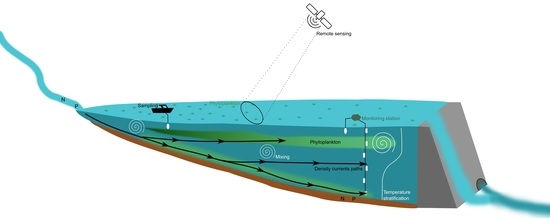
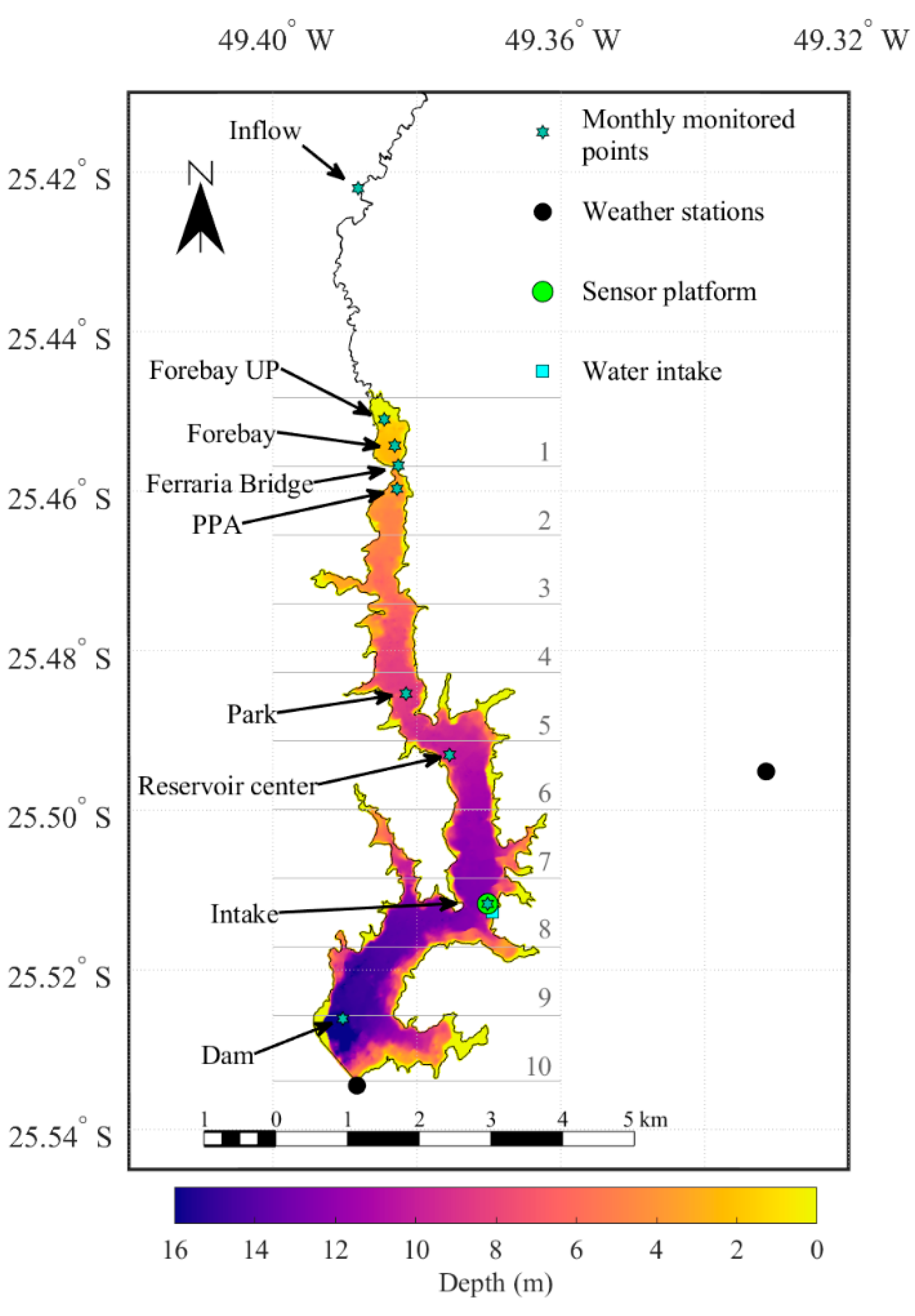
2.1. Study Site
2.2. Monitoring Program
2.2.1. Sensors
2.2.2. Laboratory Analyses
2.3. Remote Sensing Images
2.4. Reservoir Hydrodynamics
2.5. Statistical Metrics
3. Results
3.1. Continuous Observations
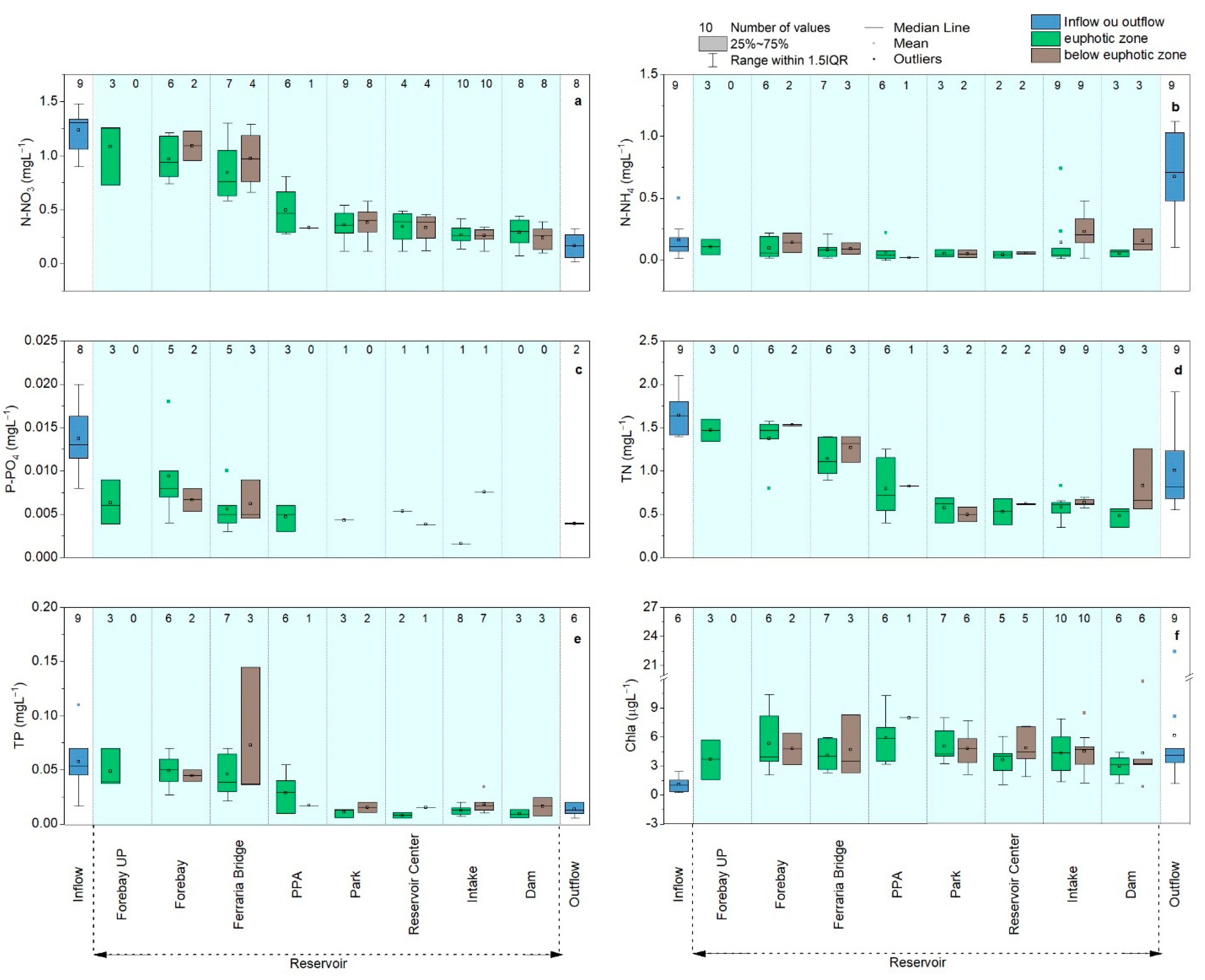
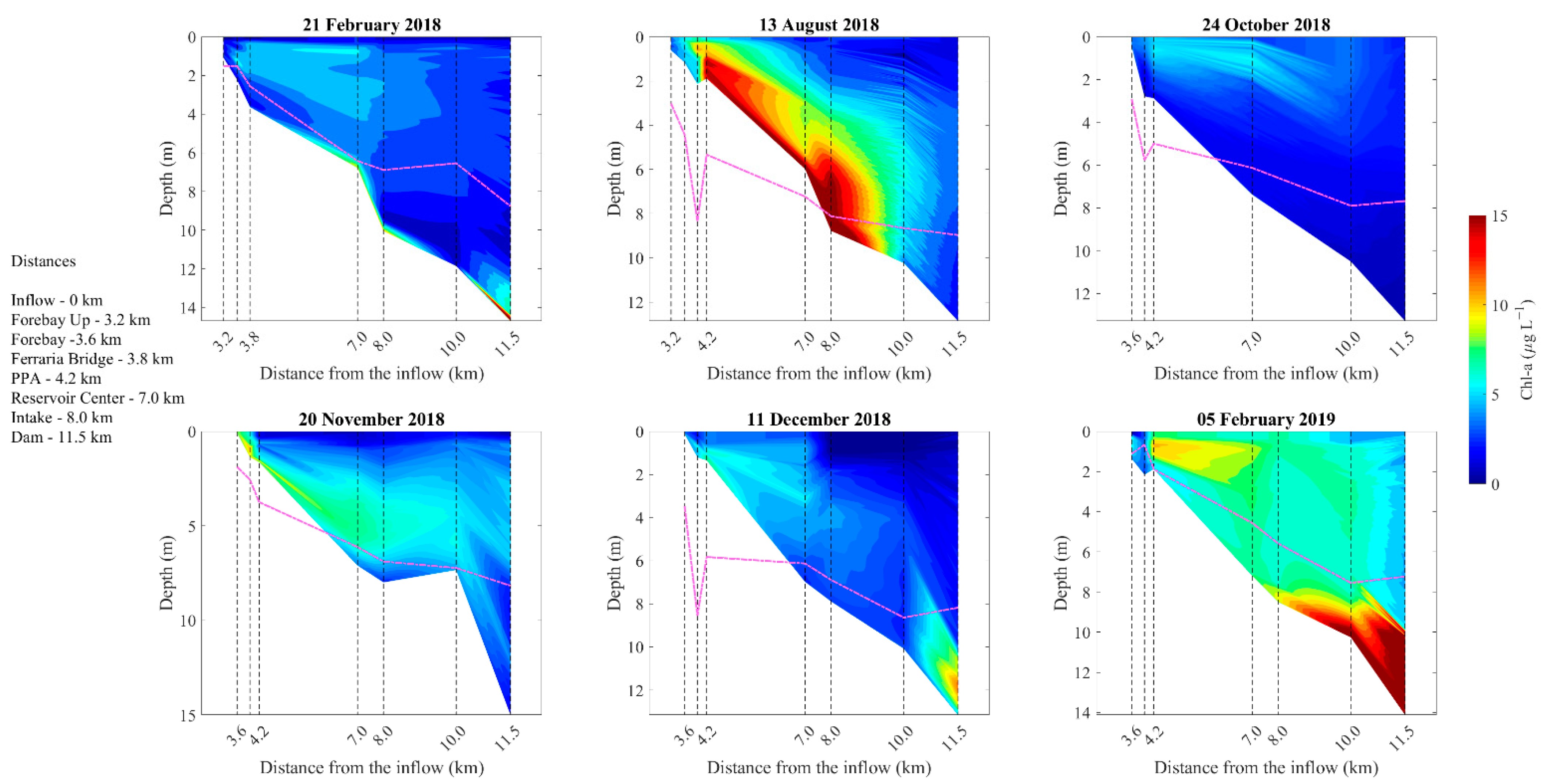
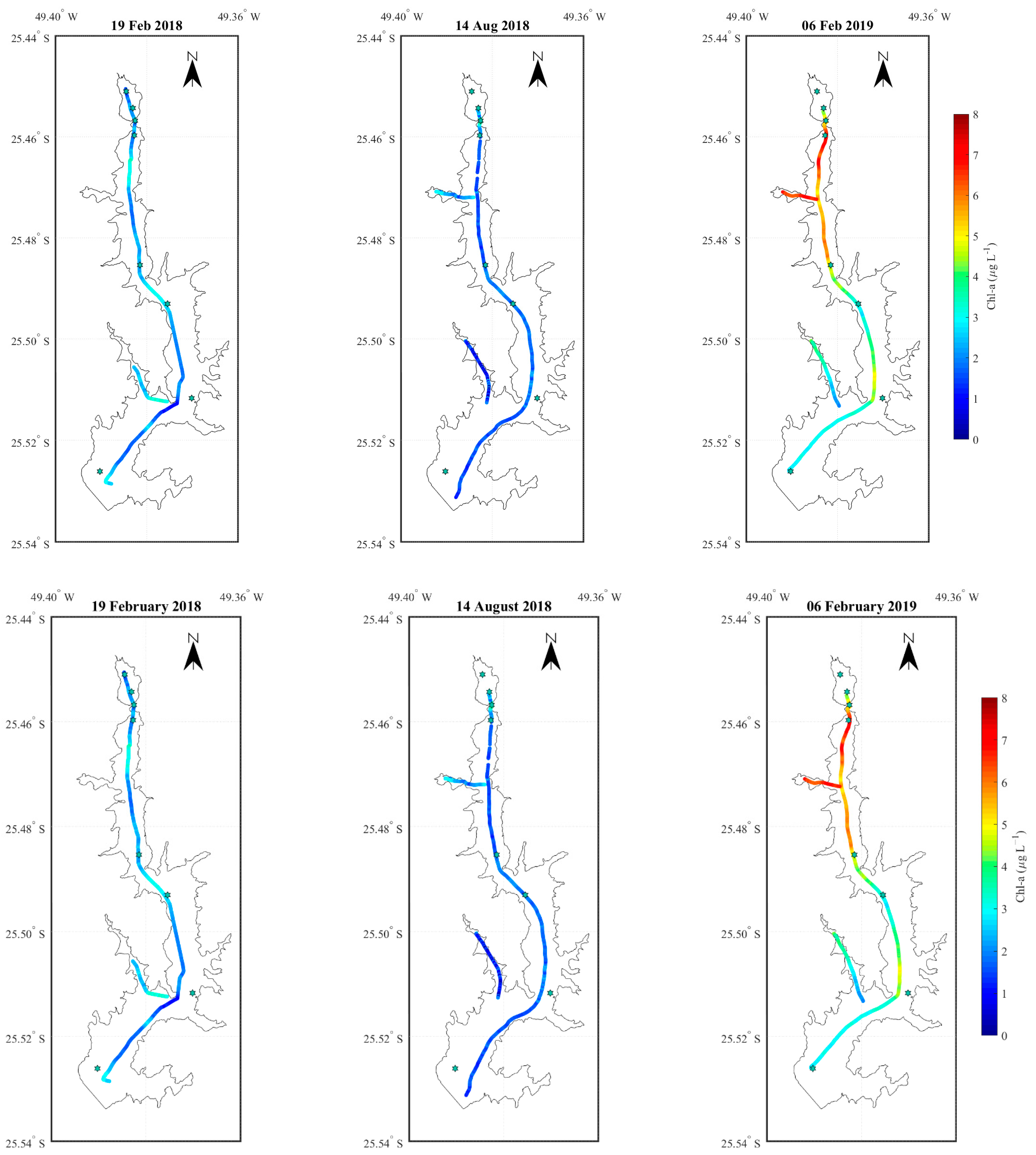
3.2. Longitudinal Variations
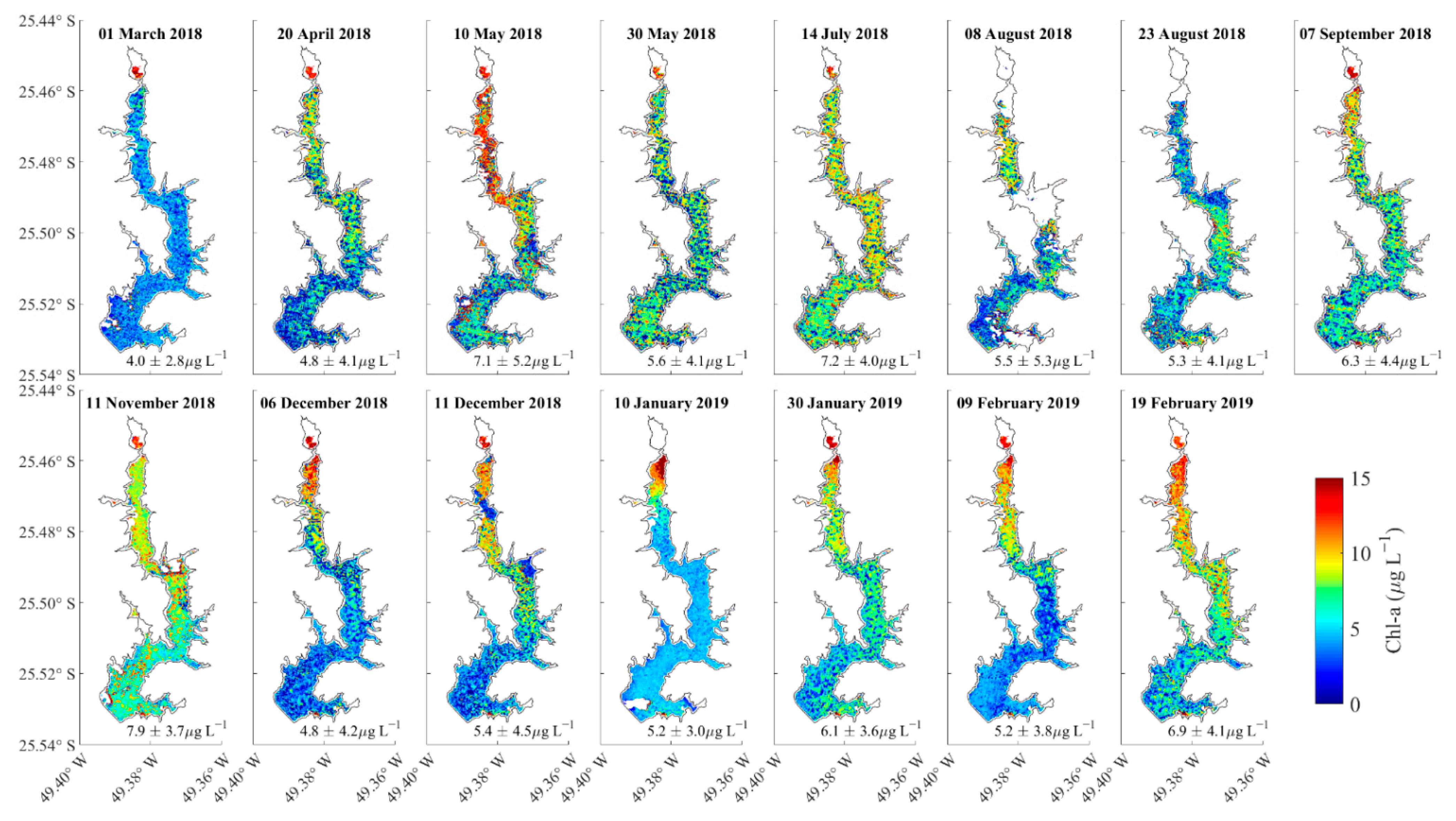
3.3. Spatial Variations of Chla at the Water Surface
3.4. Linking Water Quality to Physical Processes
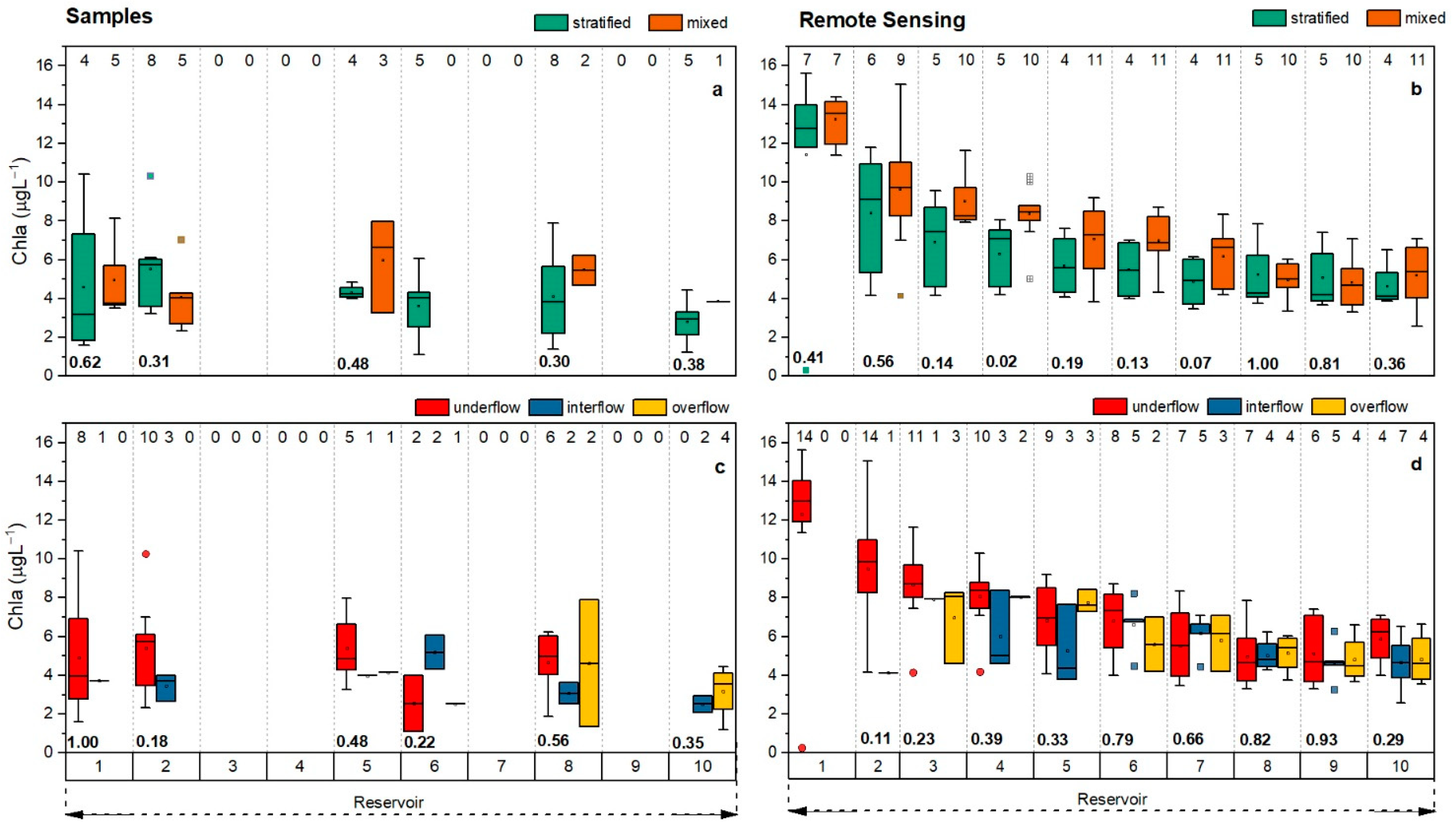
3.4.1. Temporal and Spatial Variations
3.4.2. Correlations
4. Discussion
4.1. Temporal and Spatial Variations of Nutrients and Chlorophyll
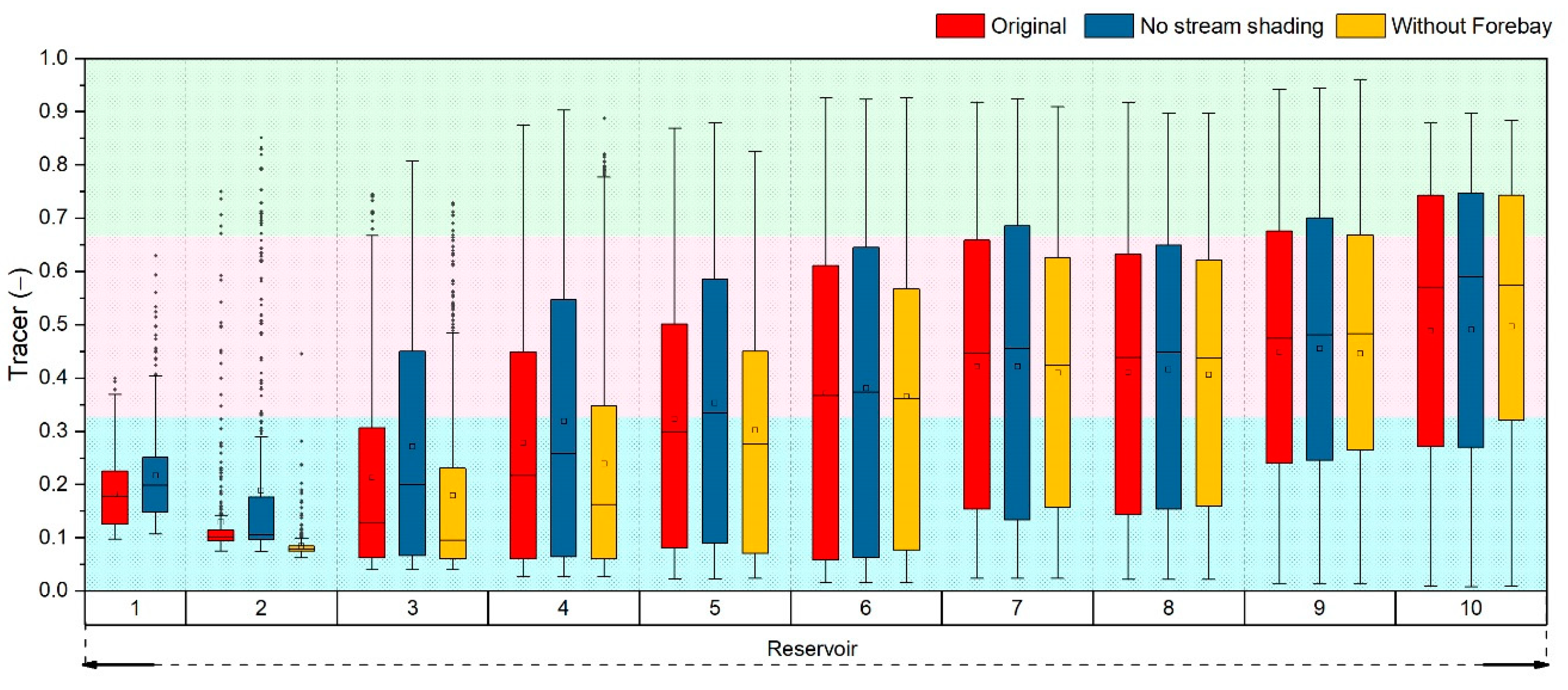
4.2. Effects of Density Currents
4.3. Correlations between Nutrient and Chlorophyll Concentrations
5. Conclusions
Supplementary Materials
Author Contributions
Funding
Data Availability Statement
Acknowledgments
Conflicts of Interest
References
- Klippel, G.; Macêdo, R.L.; Branco, C.W.C. Comparison of different trophic state indices applied to tropical reservoirs. LakesReserv. Sci. Policy Manag. Sustain. Use 2020, 25, 214–229. [Google Scholar] [CrossRef]
- Cunha, D.G.F.; Finkler, N.R.; Lamparelli, M.C.; Calijuri, M.d.C.; Dodds, W.K.; Carlson, R.E. Characterizing Trophic State in Tropical/Subtropical Reservoirs: Deviations among Indexes in the Lower Latitudes. Environ. Manag. 2021, 68, 491–504. [Google Scholar] [CrossRef]
- Megard, R.O. Phytoplankton, Photosynthesis, And Phosphorus In Lake Minnetonka, Minnesota1. Limnol. Oceanogr. 1972, 17, 68–87. [Google Scholar] [CrossRef]
- Havens, K.E.; Nürnberg, G.K. The Phosphorus-Chlorophyll Relationship in Lakes: Potential Influences of Color and Mixing Regime. Lake Reserv. Manag. 2004, 20, 188–196. [Google Scholar] [CrossRef]
- Dillon, P.J.; Rigler, F.H. The phosphorus-chlorophyll relationship in lakes1,2. Limnol. Oceanogr. 1974, 19, 767–773. [Google Scholar] [CrossRef]
- Phillips, G.; Pietiläinen, O.P.; Carvalho, L.; Solimini, A.; Lyche Solheim, A.; Cardoso, A.C. Chlorophyll–nutrient relationships of different lake types using a large European dataset. Aquat. Ecol. 2008, 42, 213–226. [Google Scholar] [CrossRef] [Green Version]
- Stow, C.A.; Cha, Y. Are Chlorophyll a–Total Phosphorus Correlations Useful for Inference and Prediction? Environ. Sci. Technol. 2013, 47, 3768–3773. [Google Scholar] [CrossRef]
- Quinlan, R.; Filazzola, A.; Mahdiyan, O.; Shuvo, A.; Blagrave, K.; Ewins, C.; Moslenko, L.; Gray, D.K.; O’Reilly, C.M.; Sharma, S. Relationships of total phosphorus and chlorophyll in lakes worldwide. Limnol. Oceanogr. 2021, 66, 392–404. [Google Scholar] [CrossRef]
- Abell, J.M.; Özkundakci, D.; Hamilton, D.P.; Jones, J.R. Latitudinal variation in nutrient stoichiometry and chlorophyll-nutrient relationships in lakes: A global study. Fundam. Appl. Limnol. 2012, 181, 1–14. [Google Scholar] [CrossRef]
- Filstrup, C.T.; Wagner, T.; Soranno, P.A.; Stanley, E.H.; Stow, C.A.; Webster, K.E.; Downing, J.A. Regional variability among nonlinear chlorophyll—phosphorus relationships in lakes. Limnol. Oceanogr. 2014, 59, 1691–1703. [Google Scholar] [CrossRef]
- Shuvo, A.; O’Reilly, C.M.; Blagrave, K.; Ewins, C.; Filazzola, A.; Gray, D.; Mahdiyan, O.; Moslenko, L.; Quinlan, R.; Sharma, S. Total phosphorus and climate are equally important predictors of water quality in lakes. Aquat. Sci. 2021, 83, 16. [Google Scholar] [CrossRef]
- Lewis, W.M., Jr. Tropical lakes: How latitude makes a difference. In Perspectives in Tropical Limnology; SPB Academic Publishing: Amsterdam, The Netherlands, 1996; Volume 4364. [Google Scholar]
- Winton, R.S.; Calamita, E.; Wehrli, B. Reviews and syntheses: Dams, water quality and tropical reservoir stratification. Biogeosciences 2019, 16, 1657–1671. [Google Scholar] [CrossRef] [Green Version]
- Mulligan, M.; van Soesbergen, A.; Sáenz, L. GOODD, a global dataset of more than 38,000 georeferenced dams. Sci. Data 2020, 7, 31. [Google Scholar] [CrossRef] [Green Version]
- Zarfl, C.; Lumsdon, A.E.; Berlekamp, J.; Tydecks, L.; Tockner, K. A global boom in hydropower dam construction. Aquat. Sci. 2014, 77, 161–170. [Google Scholar] [CrossRef]
- Yasarer, L.M.W.; Sturm, B.S.M. Potential impacts of climate change on reservoir services and management approaches. Lake Reserv. Manag. 2016, 32, 13–26. [Google Scholar] [CrossRef]
- Fadel, A.; Sharaf, N.; Siblini, M.; Slim, K.; Kobaissi, A. A simple modelling approach to simulate the effect of different climate scenarios on toxic cyanobacterial bloom in a eutrophic reservoir. Ecohydrol. Hydrobiol. 2019, 19, 359–369. [Google Scholar] [CrossRef]
- Weber, C.J.; Weihrauch, C. Autogenous Eutrophication, Anthropogenic Eutrophication, and Climate Change: Insights from the Antrift Reservoir (Hesse, Germany). Soil Syst. 2020, 4, 29. [Google Scholar] [CrossRef]
- Kimmel, B.L.; Lind, O.T.; Paulson, L.J. Reservoir primary productivity. In Reservoir Limnology: Ecological Perspectives; John Wiley & Sons, Inc.: Hoboken, NJ, USA, 1990; Volume 1, pp. 133–199. [Google Scholar]
- Kimmel, B.L.; Groeger, A.W. Factors Controlling Primary Production In Lakes And Reservoirs: A Perspective. Lake Reserv. Manag. 1984, 1, 277–281. [Google Scholar] [CrossRef]
- Noori, R.; Ansari, E.; Jeong, Y.-W.; Aradpour, S.; Maghrebi, M.; Hosseinzadeh, M.; Bateni, S.M. Hyper-Nutrient Enrichment Status in the Sabalan Lake, Iran. Water 2021, 13, 2874. [Google Scholar] [CrossRef]
- Sun, H.; Lu, X.; Yu, R.; Yang, J.; Liu, X.; Cao, Z.; Zhang, Z.; Li, M.; Geng, Y. Eutrophication decreased CO2 but increased CH4 emissions from lake: A case study of a shallow Lake Ulansuhai. Water Res. 2021, 201, 117363. [Google Scholar] [CrossRef]
- Gholizadeh, M.H.; Melesse, A.M.; Reddi, L. A Comprehensive Review on Water Quality Parameters Estimation Using Remote Sensing Techniques. Sensors 2016, 16, 1298. [Google Scholar] [CrossRef] [PubMed] [Green Version]
- Rueda, F.J.; Fleenor, W.E.; de Vicente, I. Pathways of river nutrients towards the euphotic zone in a deep-reservoir of small size: Uncertainty analysis. Ecol. Model. 2007, 202, 345–361. [Google Scholar] [CrossRef]
- Cortés, A.; Fleenor, W.; Wells, M.; de Vicente, I.; Rueda, F. Pathways of river water to the surface layers of stratified reservoirs. Limnol. Oceanogr. 2014, 59, 233–250. [Google Scholar] [CrossRef]
- Ishikawa, M.; Haag, I.; Krumm, J.; Teltscher, K.; Lorke, A. The effect of stream shading on the inflow characteristics in a downstream reservoir. River Res. Appl. 2021, 37, 943–954. [Google Scholar] [CrossRef]
- Sanepar, C.d.S.d.P. Plano Diretor SAIC: Sistema de Abastecimento de Água Integrado de Curitiba e Região Metropolitana. Curitiba Sanepar 2013. Available online: https://site.sanepar.com.br/arquivos/saicplanodiretor.pdf (accessed on 30 September 2020).
- Sotiri, K.; Hilgert, S.; Fuchs, S. Sediment classification in a Brazilian reservoir: Pros and cons of parametric low frequencies. Adv. Oceanogr. Limnol. 2019, 10. [Google Scholar] [CrossRef]
- Luhtala, H.; Tolvanen, H. Optimizing the Use of Secchi Depth as a Proxy for Euphotic Depth in Coastal Waters: An Empirical Study from the Baltic Sea. ISPRS Int. J. Geo-Inf. 2013, 2, 1153–1168. [Google Scholar] [CrossRef]
- Rousso, B.Z.; Bertone, E.; Stewart, R.A.; Rinke, K.; Hamilton, D.P. Light-induced fluorescence quenching leads to errors in sensor measurements of phytoplankton chlorophyll and phycocyanin. Water Res. 2021, 198, 117133. [Google Scholar] [CrossRef]
- APHA. Standard Methods for the Examination of Water and Wastewater, 21st ed.; American Public Health Association: Washington, DC, USA, 2005. [Google Scholar]
- COMPANHIA AMBIENTAL DO ESTADO DE SÃO PAULO (CETESB). L5.306: Determinação de Clorofila a e Feofitina a: Método Espectrofotométrico, 3rd ed.; Companhia Ambiental do Estado de São Paulo: São Paulo, Brazil, 2014. [Google Scholar]
- Brockmann, C.; Doerffer, R.; Peters, M.; Kerstin, S.; Embacher, S.; Ruescas, A. Evolution of the C2RCC Neural Network for Sentinel 2 and 3 for the Retrieval of Ocean Colour Products in Normal and Extreme Optically Complex Waters. In Proceedings of the conference: Living Planet Symposium 2016, Prague, Czech Republic, 1 August 2016; p. 54. [Google Scholar]
- Ishikawa, M.; Bleninger, T.; Lorke, A. Hydrodynamics and mixing mechanisms in a subtropical reservoir. Inland Waters 2021, 11, 286–301. [Google Scholar] [CrossRef]
- Ishikawa, M.; Gonzalez, W.; Golyjeswski, O.; Sales, G.; Rigotti, J.A.; Bleninger, T.; Mannich, M.; Lorke, A. Effects of dimensionality on the performance of hydrodynamic models for stratified lakes and reservoirs. Geosci. Model Dev. 2022, 15, 2197–2220. [Google Scholar] [CrossRef]
- Wetzel, R.G. Limnology: Lake and River Ecosystems; Academic Press: San Diego, CA, USA; London, UK, 2001. [Google Scholar]
- de Oliveira, T.F.; de Sousa Brandão, I.L.; Mannaerts, C.M.; Hauser-Davis, R.A.; Ferreira de Oliveira, A.A.; Fonseca Saraiva, A.C.; de Oliveira, M.A.; Ishihara, J.H. Using hydrodynamic and water quality variables to assess eutrophication in a tropical hydroelectric reservoir. J. Environ. Manag. 2020, 256, 109932. [Google Scholar] [CrossRef]
- Shatwell, T.; Adrian, R.; Kirillin, G. Planktonic events may cause polymictic-dimictic regime shifts in temperate lakes. Sci. Rep. 2016, 6, 24361. [Google Scholar] [CrossRef] [Green Version]
- Soranno, P.A.; Carpenter, S.R.; Lathrop, R.C. Internal phosphorus loading in Lake Mendota: Response to external loads and weather. Can. J. Fish. Aquat. Sci. 1997, 54, 1883–1893. [Google Scholar] [CrossRef]
- Mesman, J.P.; Ayala, A.I.; Goyette, S.; Kasparian, J.; Marcé, R.; Markensten, H.; Stelzer, J.A.A.; Thayne, M.W.; Thomas, M.K.; Pierson, D.C.; et al. Drivers of phytoplankton responses to summer wind events in a stratified lake: A modeling study. Limnol. Oceanogr. 2022, 67, 856–873. [Google Scholar] [CrossRef]
- Lewis Jr., W. Biogeochemistry of tropical lakes. Int. Ver. fÜR Theor. Angew.Limnol. Verh. 2010, 30, 1595–1603. [Google Scholar] [CrossRef]
- Sterner, R.W. On the Phosphorus Limitation Paradigm for Lakes. Int. Rev. Hydrobiol. 2008, 93, 433–445. [Google Scholar] [CrossRef]
- Caputo, L.; Naselli-Flores, L.; OrdoÑEz, J.; Armengol, J. Phytoplankton distribution along trophic gradients within and among reservoirs in Catalonia (Spain). Freshw. Biol. 2008, 53, 2543–2556. [Google Scholar] [CrossRef]
- Rychtecký, P.; Znachor, P. Spatial heterogeneity and seasonal succession of phytoplankton along the longitudinal gradient in a eutrophic reservoir. Hydrobiologia 2011, 663, 175–186. [Google Scholar] [CrossRef]
- Gomes Nogueira, M. Phytoplankton composition, dominance and abundance as indicators of environmental compartmentalization in Jurumirim Reservoir (Paranapanema River), São Paulo, Brazil. Hydrobiologia 2000, 431, 115–128. [Google Scholar] [CrossRef]
- Freire, R.; Calijuri, M.; Santaella, S. Longitudinal patterns and variations in water quality in a reservoir in the semiarid region of NE Brazil: Responses to hydrological and climatic changes. Acta Limnol. Bras. 2009, 21, 251–262. [Google Scholar]
- de Moura-Júnior, E.G.; Severi, W.; Kamino, L.H.Y.; de Lemos-Filho, J.P. To what degree do spatial and limnological predictors explain the occurrence of a submerged macrophyte species in lotic and semi-lotic/lentic environments of a dammed river? Limnology 2021, 22, 101–110. [Google Scholar] [CrossRef]
- Soomets, T.; Uudeberg, K.; Jakovels, D.; Brauns, A.; Zagars, M.; Kutser, T. Validation and Comparison of Water Quality Products in Baltic Lakes Using Sentinel-2 MSI and Sentinel-3 OLCI Data. Sensors 2020, 20, 742. [Google Scholar] [CrossRef] [Green Version]
- Ogashawara, I.; Kiel, C.; Jechow, A.; Kohnert, K.; Ruhtz, T.; Grossart, H.-P.; Hölker, F.; Nejstgaard, J.C.; Berger, S.A.; Wollrab, S. The Use of Sentinel-2 for Chlorophyll-a Spatial Dynamics Assessment: A Comparative Study on Different Lakes in Northern Germany. Remote Sens. 2021, 13, 1542. [Google Scholar] [CrossRef]
- Owens, E.M.; Effler, S.W.; O’Donnell, D.M.; Matthews, D.A. Modeling the Fate and Transport of Plunging Inflows to Onondaga Lake. JAWRA J. Am. Water Resour. Assoc. 2014, 50, 205–218. [Google Scholar] [CrossRef]
- Sotiri, K.; Hilgert, S.; Mannich, M.; Bleninger, T.; Fuchs, S. Implementation of comparative detection approaches for the accurate assessment of sediment thickness and sediment volume in the Passaúna Reservoir. J. Environ. Manag. 2021, 287, 112298. [Google Scholar] [CrossRef]
- Marcon, L.; Sotiri, K.; Bleninger, T.; Lorke, A.; Männich, M.; Hilgert, S. Acoustic Mapping of Gas Stored in Sediments of Shallow Aquatic Systems Linked to Methane Production and Ebullition Patterns. Front. Environ. Sci. 2022, 10. [Google Scholar] [CrossRef]
- Hutchinson, G.E. On the Relation between the Oxygen Deficit and the productivity and Typology of Lakes. Int. Rev. Gesamten Hydrobiol. Hydrogr. 1938, 36, 336–355. [Google Scholar] [CrossRef]
- Müller, B.; Bryant, L.D.; Matzinger, A.; Wüest, A. Hypolimnetic Oxygen Depletion in Eutrophic Lakes. Environ. Sci. Technol. 2012, 46, 9964–9971. [Google Scholar] [CrossRef]
- Carneiro, F.M.; Nabout, J.C.; Vieira, L.C.G.; Roland, F.; Bini, L.M. Determinants of chlorophyll-a concentration in tropical reservoirs. Hydrobiologia 2014, 740, 89–99. [Google Scholar] [CrossRef]
- Chen, G.; Fang, X.; Devkota, J. Understanding flow dynamics and density currents in a river-reservoir system under upstream reservoir releases. Hydrol. Sci. J. 2016, 61, 2411–2426. [Google Scholar] [CrossRef] [Green Version]


| Equipment | Fluorometer | Spectrometer | Fluorometer | Conductivity, Temperature, and Depth Profiler |
|---|---|---|---|---|
| Equipment model | nanoFlu | OPUS | FluoroProbe III | CastAway-CTD |
| Manufacturer | TriOS | TriOS | bbe moldaenke | Sontek |
| Origin | Rastede, Germany | Rastede, Germany | Schwentinental, Germany | San Diego, United States |
| Variables measured | chla | Nitrate(N-NO3) | chla with the determination of algae classes | conductivity, temperature, and depth |
| Range | 0 to 200 µg L−1 | 0.03 to 10 mg L−1 | 0 to 500 µg L−1 | |
| AccuracyResolution | ±5% | ±5% | 0.01 µg L−1 | 0.1 PSU and 0.05 °C |
| Measurements | continuous time series | continuous time series | continuous time series, longitudinal transects, and vertical profiles | Vertical profiles |
| Temporal resolution | 15 min | 15 min | for continuous measurement 1 h, and 1 s for transects and profiles | Sampling in a rate of 5 Hz. |
Publisher’s Note: MDPI stays neutral with regard to jurisdictional claims in published maps and institutional affiliations. |
© 2022 by the authors. Licensee MDPI, Basel, Switzerland. This article is an open access article distributed under the terms and conditions of the Creative Commons Attribution (CC BY) license (https://creativecommons.org/licenses/by/4.0/).
Share and Cite
Ishikawa, M.; Gurski, L.; Bleninger, T.; Rohr, H.; Wolf, N.; Lorke, A. Hydrodynamic Drivers of Nutrient and Phytoplankton Dynamics in a Subtropical Reservoir. Water 2022, 14, 1544. https://doi.org/10.3390/w14101544
Ishikawa M, Gurski L, Bleninger T, Rohr H, Wolf N, Lorke A. Hydrodynamic Drivers of Nutrient and Phytoplankton Dynamics in a Subtropical Reservoir. Water. 2022; 14(10):1544. https://doi.org/10.3390/w14101544
Chicago/Turabian StyleIshikawa, Mayra, Luziadne Gurski, Tobias Bleninger, Harald Rohr, Nils Wolf, and Andreas Lorke. 2022. "Hydrodynamic Drivers of Nutrient and Phytoplankton Dynamics in a Subtropical Reservoir" Water 14, no. 10: 1544. https://doi.org/10.3390/w14101544
APA StyleIshikawa, M., Gurski, L., Bleninger, T., Rohr, H., Wolf, N., & Lorke, A. (2022). Hydrodynamic Drivers of Nutrient and Phytoplankton Dynamics in a Subtropical Reservoir. Water, 14(10), 1544. https://doi.org/10.3390/w14101544