Sustainable Water Allocation in Umarkhed Taluka through Optimization of Reservoir Operation in the Wardha Sub-Basin, India

Abstract

Climate change is causing shifts in seasonal weather patterns and variation in seasonal time scales in India. Factors including uneven distribution of water, faulty agricultural practices and water policies, low prices of farm products, and debt are leading farmers to commit suicide in Umarkhed Taluka of the Yavatmal District. This study aimed to develop a sustainable solution to water scarcity in the surrounding watershed by introducing optimization modeling in reservoir operation. Past studies have conducted different hydrologic analyses to address the water scarcity issue in this region. However, none of the studies incorporated optimization in their models. This study developed an integrated hydrologic and optimization model that can predict the daily reservoir releases for climate change scenarios from 2020 to 2069 based upon Representative Concentration Pathway (RCP-4.5 and RCP-8.5) climate change scenarios from 2020 to 2069. The integrated simulations were able to deliver around 19% more water than the historical discharge at the most downstream station of the Wardha Watershed. The simulated approaches store less water than the actual unoptimized scenario and deliver water when there is a need at the downstream locations. Finally, because the downstream locations of the Wardha Watershed receive more water, a localized storage system can be developed and a transfer method can be utilized to deliver sufficient water to the Umarkhed Taluka.

1. Introduction

In recent years, shifts in seasonal weather patterns due to climate change have caused unexpected variations in rainfall in Umarkhed Taluka, an agricultural-based region located in the Wardha Watershed in Godavari River Basin, India (shown in Figure 1). Recurring droughts have caused significant suffering in this region of the Wardha Watershed. Both rainfall intensities and the number of rainy days have decreased during recent decades in the Godavari River Basin [1]. In addition to recurring droughts, the main challenges for farmers are considered to be unequal supply of water, education, and knowledge of efficient farming. An additional outcome is a higher suicide rate [2,3].

1.1. Previous Studies of Umarkhed

No studies have been performed that have considered the optimization of the reservoir operations in the Wardha Watershed to mitigate the water scarcity issue in the Umarkhed region by utilizing appropriate reservoir release predictions. Instead, studies have concentrated on various actions, such as land use pattern changes, repairing existing water storage tanks, and constructing water storage tanks to reduce the consequences of water scarcity.

Sowjanya et al. [4] analyzed future rainfall predictions for different Representative Concentration Pathway scenarios (which are a new category of climate prediction process introduced in 2014) and concluded that land use patterns need to be developed that reduce the consequences of water scarcity. Studies of the water scarcity of the Umarkhed region have also been performed. These include that of Gujja et al. [5], who suggested constructing more water tanks to store water. A small number of researchers, including Garg et al. [6] and Sowjanya et al. [4], conducted their studies on the rainfall patterns resulting from climate change, and concluded that it is extremely difficult to completely address the water quantity problem in this region.

There appears to be a strong correlation between climate, food, and water crises. Accordingly, climate change transforms the amount and timing of precipitation, which determines the amount of water available for irrigation use in agriculture [5].

Different researchers have tried to address the problem of water scarcity in the Godavari Basin region. Gujja et al. [5] mentioned the importance of developing water-storing technologies to mitigate the ongoing catastrophe of lack of water availability. However, researchers have shown more interest in reinstating water tanks than building dams and reservoirs. According to the World Bank, there are about 74,000 water tanks in Andhra Pradesh, some of which were built more than 2000 years ago [5]. About 6234 water tanks in the Maner sub-basin of Godavari cover 5% of its area. About 5.6 hectors of irrigation land can be served by a water tank having a size of 1 hectare. Gujja et al. [5] claimed that repairing existing water tanks is the optimal solution to the issue of managing future water resources. In another study, during the water resource assessment of the Godavari River basin, Garg et al. [6] concluded that the varied rainfall pattern has made it impossible to supply enough water to locations upstream of the basin.

Sowjanya et al. [4] studied the streamflow variations of the Wardha Watershed for RCP 4.5 and 8.5 conditions and simulated them with the Soil and Water Assessment Tool (SWAT). The authors compared different climate models, namely, ACCESS, CCSM, CNRM, NorESM, and MPI-ESM-LR, with the observed data. The models were calibrated and evaluated for the period from 1984 to 2003. Analyzing the predicted precipitation and stream flows, the authors concluded that the observed changes in water balance components are due to climate change and can only be addressed by improving the land use and land cover of this basin.

According to Tupe and Joshi [7], cotton is the most important crop that largely grows during rain (Kharif season) in the area surrounding Umarkhed. Moreover, soybean, pigeon pea, sorghum, green pea, black gram, etc., also grow during this season. However, wheat and chickpea are cultivated during winter (Rabi season). Godavari has a significant number of forests in central India that are homes to the Royal Bengal tigers, elephants, and other species. The forests are also homes of other endangered fauna [8].

1.2. Climate Change and Water Scarcity

Gosain et al. [9] conducted a study that aimed to identify the impacts of climate change on Indian flowing water bodies. The authors analyzed precipitation, temperature, solar radiation, wind speed, and relative humidity data of all Indian river basins. The study results predicted a future scenario (2041–2060) with regards to greenhouse gas (GHG) emissions, which is a major element of climate change in Indian basins. The study explained that the GHG scenario may cause severe droughts in some parts of India, whereas other areas may be affected by frequent floods. Although Gosain et al. [9] predicted that sub-basins of Godavari will face flooding rather than water scarcity, many parts of the Godavari River Basin have been affected by intense droughts in recent years.

The Intergovernmental Panel on Climate Change (IPCC) introduced new categories of climate prediction, named the Representative Concentration Pathways. These prediction processes consider the greenhouse gas emission trajectory of the 21st century as the key parameter. They classified these processes according to their peak radiative forcing value in $\mathrm{W}/{\mathrm{m}}^2$. Among these scenarios, RCP-2.6 predicts the fastest recovery of the climate. This scenario achieves a maximum value of radiative forcing of around 3 $\mathrm{W}/{\mathrm{m}}^2$, which subsequently declines gradually. For RCP-4.5, the peak value is 4.5 $\mathrm{W}/{\mathrm{m}}^2$. This value remains stable throughout the century. For RCP-8.5, the radiative forcing curve continues to increase throughout the entire century and achieves the maximum value of 8.5 $\mathrm{W}/{\mathrm{m}}^2$. Das and Umamahesh [10] investigated future rainfall patterns of the Godavari River Basin for different Representative Concentration Pathways scenarios. The peaks of greenhouse gas emissions are achieved around 2010 for RCP-2.6 and around 2040 for RCP-4.5 [10].

1.3. Study Objective

The current study examined a sustainable solution to mitigate the water scarcity issue in the Umarkhed region by utilizing appropriate reservoir release predictions. The objective of this study was to develop sustainable solutions for the water scarcity of the region through a simulation–optimization modeling approach that considered climate change scenarios. To accomplish this, an integrated hydrologic rainfall-runoff modeling and optimization modeling approach was utilized to predict daily reservoir release operations for climate change scenarios from 2020 to 2069. The hydrologic modeling included developing a rainfall-runoff model of the region using the U.S. Army Corps of Engineers HEC-HMS. The optimization model, which was developed in General Algebraic Modeling System (GAMS) determines the reservoir releases from two reservoirs in the region.

The study developed a hydrologic basin model which was calibrated according to the historical discharge patterns. Subsequently, the reservoir releases for future predicted scenarios were optimized through GAMS. Finally, the optimized discharge patterns of different downstream stations of this watershed elaborated how efficiently the estimated model will be able to address the issue of water scarcity in Umarkhed.

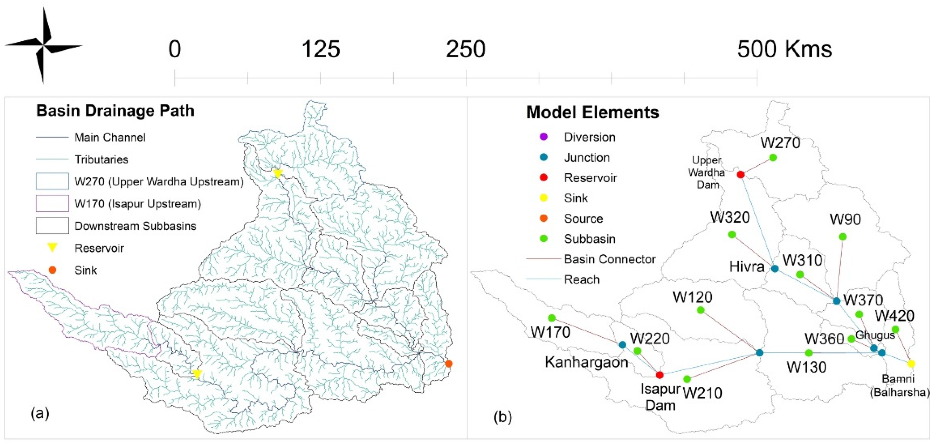
2. Modeling Methodology

The current analysis was conducted by preparing a hydrologic basin model in HEC-HMS (see Section 2.2), calibrating the basin parameters according to the historical discharge patterns (Section 2.3), and optimizing the reservoir releases for future predicted scenarios to improve the water allocation using the GAMS optimization software (see Section 2.4). Finally, the optimized discharge patterns of different downstream stations of this watershed elaborated how efficiently the estimated model will be able to address the issue of water scarcity at Umarkhed.

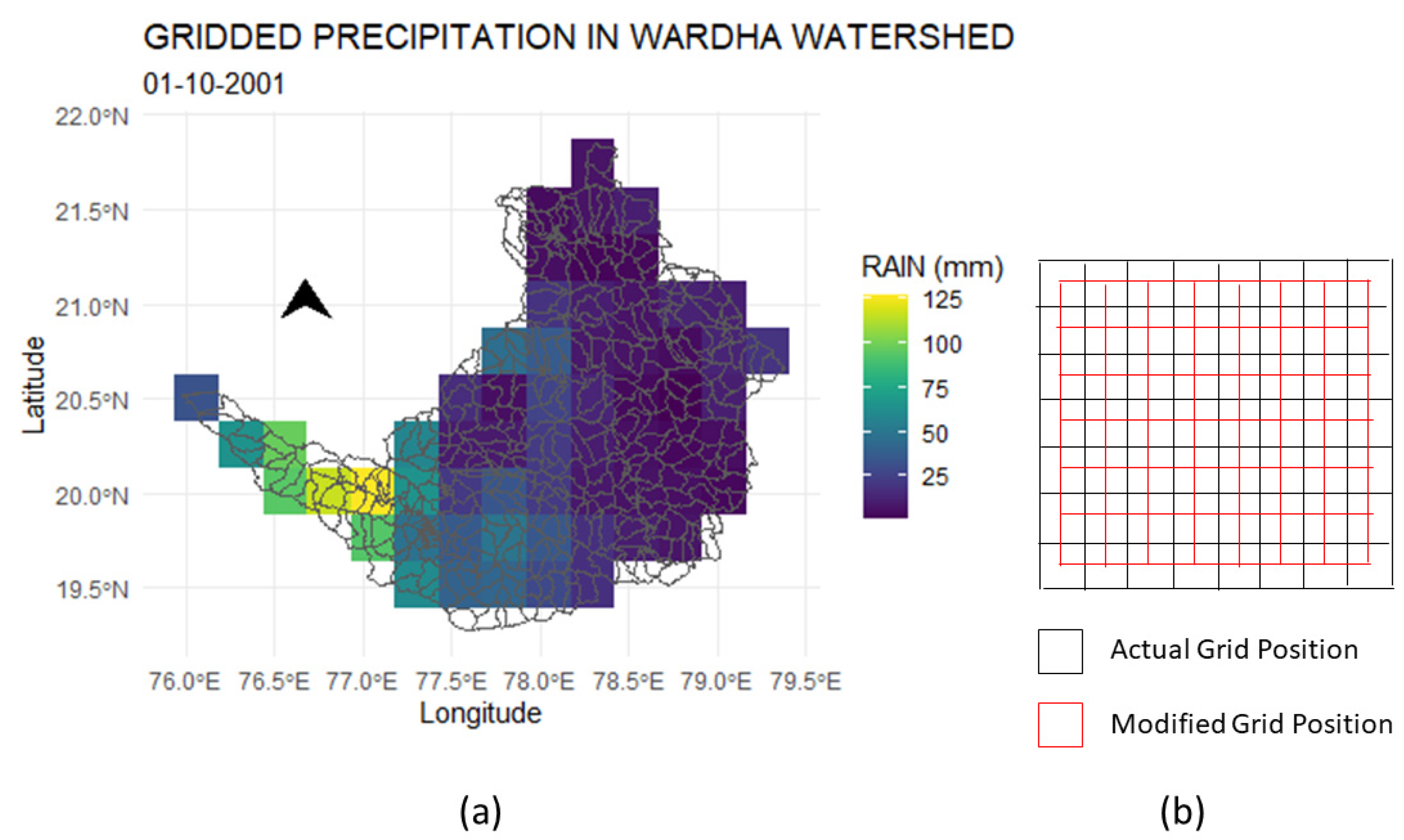
2.1. Model Data and Assumptions

A hydrologic model requires basic watershed input parameters, namely, historical discharge, atmospheric data, soil, and land use pattern for model calibration and then validate the model [11]. Remotely sensed satellite-based data were collected as raster files, which were then transformed to build the basin model. Subsequently, the gridded data were transformed into CSV format for use in the hydrologic model. In some cases, the historical patterns of discharge were predicted because of unavailable data.

The Digital Elevation Model (DEM) and the river network maps are the main elements required to prepare the hydrologic model using the HEC-geoHMS and Archydro tools [12]. The 30″ × 30″ resolution DEM for the surrounding continent (Asia) was collected from the NASA earth-explorer and HydroSHEDS server (see Figure 2a).

Roy et al. [13] provided land use and land cover maps of three consecutive decades (1985, 1995, and 2005), which were obtained from Oak Ridge National Laboratory Distributed Active Archive Center (ORNL DAAC). Figure 2b indicates that the majority of the areas of the Wardha Watershed region is covered with agricultural lands.

The soil cover shapefile was collected from the Food and Agricultural Organization (FAO) website, and was modified to a raster file (see Figure 2c). The hydrologic soil classes were identified using the ArcSWAT database. The data from the polygon layer of the merged soil cover and land cover maps were transferred to the hydrologic model as the input basin parameters. In this watershed, soil cover can be classified either as hydrologic class C or class D. Hydrologic class A and class B are rare in this region.

The Normalized Difference Vegetation Index (NDVI) distribution in the sub-basin area is shown in Figure 2d–g. The figures show that NDVI values are close to 0.3 for the entire region in January, April, and July. It has the maximum vegetation cover in October (start of the Rabi season), which is close to 0.5. This vegetation pattern indicates that vegetation is insufficient during most of the year in Wardha sub-basin.

The gridded rainfall time-series data (grid size: 0.25° × 0.25°) were collected from the Indian Meteorological Department (IMD) database. The netCDF files were stored as an Excel spreadsheet to incorporate them with the basin meteorological parameters. Figure 3a shows an example of rainfall patterns for the first day of the water year of 2002 (1 October 2001) in the Wardha Watershed. In this analysis, for RCP-4.5, the Norwegian Earth System Model 1 (NorSEM) climate model, which has lower intra-annual variability, was selected [7]. For RCP-8.5, the Community Climate System Model (CCSM4) was selected because it has a lower inter-annual variability [7]. These gridded data having a 0.25° grid size were collected in netCDF4 format from the Center of Climate Change Research (CCCR) of the Indian Institute of Tropical Meteorology. To align the coordinates of the daily rainfall predictions with the historical rainfall data, we transposed the grid centers via interpolation according to the historical data grids with the same resolution (see Figure 3b).

The crop water need was calculated according to the Food and Agricultural Organization training manual [14]. The percentage of different crops in Yavatmal was analyzed and multiplied by the daily evapotranspiration of each crop during different months. The total daily water requirement in a specific month was calculated by summing the active crop evapotranspiration (see Figure 4a). To model the minimum water requirement for the Wardha Watershed, we assumed an additional 5% of the irrigation water requirement downstream of the reservoirs to estimate the total water demand.

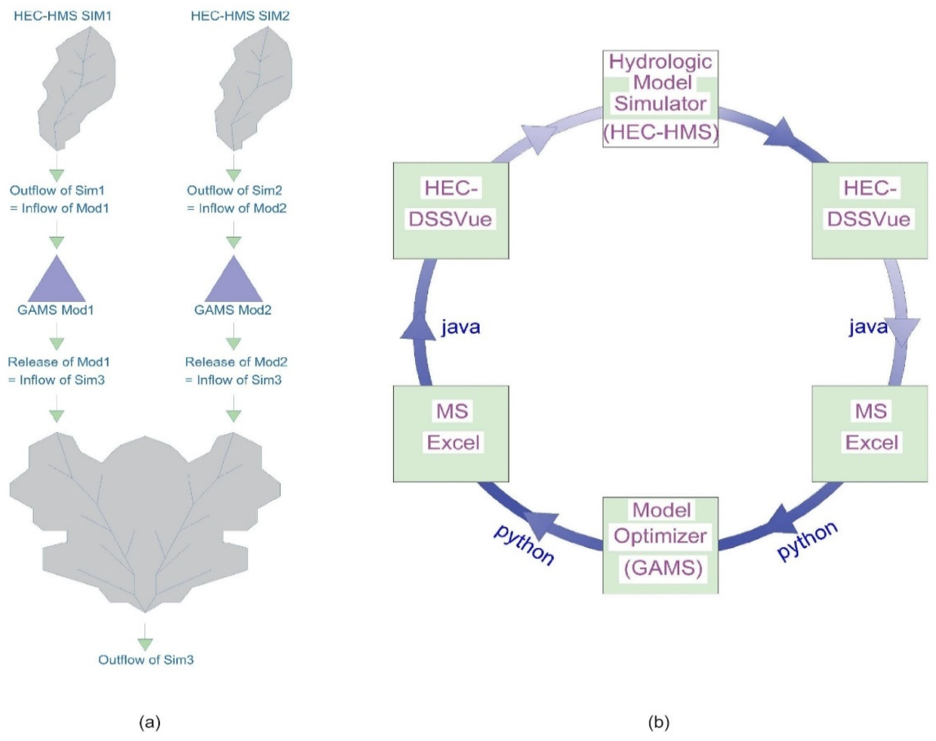
2.2. Hydrologic Model Simulation

The Hydrologic Modeling System (HEC-HMS version 3.4) was used to simulate rainfall-runoff processes in basins. HEC-HMS consists of a wide range of hydrologic elements and modeling methods. There are seven types of hydrologic elements, namely, sub-basin, reservoir, reach, junction, diversion, source, and sink, that must be considered in order to create a model in HEC-HMS. To define a model, HEC-HMS allows users to select preferred methods of parameter calculation.

In the next step, the primary basin elements were created from the Digital Elevation Model (DEM) and river stream network maps. These were generated using the HEC-GeoHMS and the Arc Hydro tools in ArcGIS. The areal separation of the Wardha sub-basin is demonstrated in Figure 5a. Moreover, Figure 5b illustrates the hydrologic model elements of the watershed.

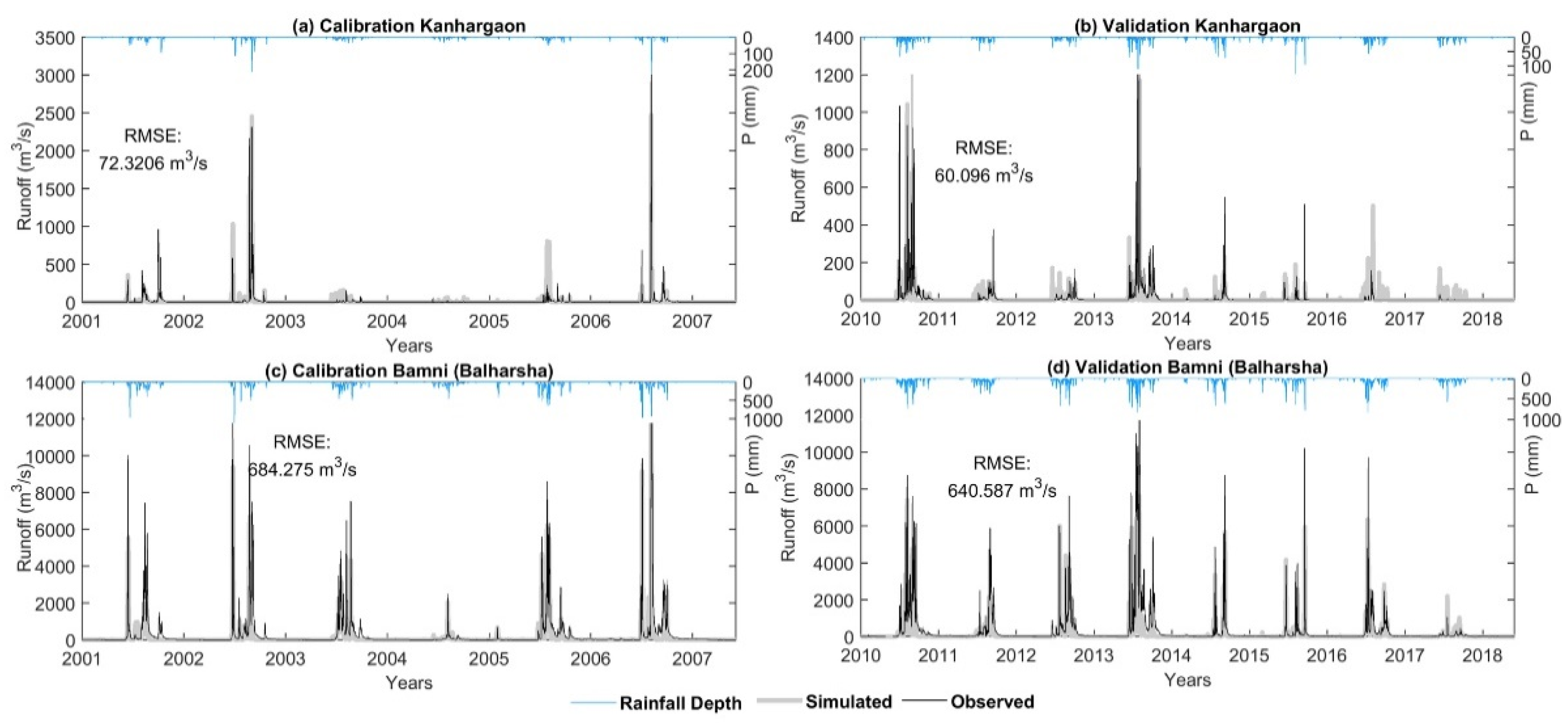
2.3. Calibration and Validation

In this study, the hydrologic model was calibrated concerning the collected station discharges as the observed datasets. According to the availability of the data, the study assembled two effective clusters of time-series from 2001 to 2007 for the calibration and 2010 to 2018 for the validation of the model. To calibrate the model, the study assumed the initial values of the parameters according to Roy et al. [16]. Roy et al. [16] studied the Soil Moisture Accounting (SMA) parameters of a neighboring catchment of the Wardha sub-basin. Initially, the Optimization Trial Tool in HEC-HMS was used to identify the appropriate values of the basin parameters. This optimization tool used Peak-Weighted Root Mean Square Error as the objective function, which minimized the weighted average distance between the simulated and observed hydrograph. The Optimization Trial Tool was unable to optimize all the basin parameters at the same time. The authors tried to identify the changing pattern of the simulated hydrograph for different values of each basin parameter. Because the observed data were available for Kanhargaon, Hivra, Ghugus, and Bamni-Balharsha, the optimized basin parameters for the upstream portions of these known stations were comparatively more accurate. These more accurate sub-basins were W170, W310, W90, and W420. Due to the minimum amount of available data at the downstream of the Isapur Dam, it was difficult to obtain the actual values of the parameters of W220, W120, W210, W360, W130, W270, W320, and W370. As a consequence, the basin parameters of the sub-basins for the less-available observed data are, comparatively, less reliable.

Table 1. Model parameters for the sub-basin, including Umarkhed (W210).

SMA Parameters	Initial Values	Final Values
Sub-basin Area (${\mathrm{km}}^2$)	10,061.2	10,061.2
Canopy storage (mm)	3	35.236
Initial Canopy Storage (%)	0	0
Surface storage (mm)	12.7	347.2
Initial Surface Storage (%)	0	9
Soil (%)	30	1
Groundwater 1 (%)	30	7
Groundwater 2 (%)	30	10
Max rate of infiltration (mm/h)	4	0.167
Impervious (%)	5	0.2196
Soil storage (mm)	400	450
Tension storage (mm)	130	130
Soil percolation (mm/h)	0.3	0.4
Groundwater 1 storage (mm)	60	130
Groundwater 1 percolation (mm/h)	0.3	0.4
Groundwater 1 coefficient (h)	90	70
Groundwater 2 storage (mm)	80	200
Groundwater 2 percolation (mm/h)	0.3	0.5
Groundwater 2 coefficient (h)	250	350
Time of Concentration (h)	24	26.925
Storage Coefficient (h)	24	15.778

provides an example of initial and final estimated values of the soil parameters for one of the watersheds of the Wardha sub-basin. The remainder of the calibrated basin parameters are provided in the Supplementary Data file.

Figure 6 compares the calibrated and the validated curves with the observed discharge hydrographs at Kanhargaon and Bamni (Balharsha) stream gauge stations, and rainfall hyetographs for the upstream sub-basins. The simulated hydrographs fluctuate with the rainfall occurrences. The hydrographs indicate the Root Mean Square Error (RMSE) values to identify the goodness-of-fit between the simulated discharge and the observed flow. Figure 6 indicates that the RMSE values at a station are similar for both the calibration and validation period. The similarities of goodness-of-fit indicate that the calibrated parameters continue to follow the observed flow pattern with similar fluctuations for the validation period, which confirms the consistency of the simulation. These calibrated basin parameters were used in this study for a future prediction timeline (2020–2069), for which the consistency of the land use and soil type pattern in the Wardha Watershed was assumed.

2.4. GAMS Optimization Model

Water resource problems are often complex and interconnected. Optimization is an important part of this complex system analysis that is often used for basin calibration or reservoir release operation. It estimates the best values of system design and operating policy variables for best system performance [17]. General Algebraic Modeling System (GAMS) is a mathematical programming and optimization modeling system with a language compiler and different solvers. It is capable of using multidimensional, large, and sparsely structured partial derivatives, and relational algebra [18]. It helps modelers to translate a real-life problem into computer code to make it understandable and solvable. GAMS can formulate different mathematical model types, namely, linear, nonlinear, mixed-integer, mixed-integer nonlinear, and mixed complementary.

2.4.1. The Hydrologic Concept behind the Model

The objective of the optimization model is to maximize the outflow of the reservoirs. Because we know the inflow and the changing storage of the reservoirs, we can use the hydrologic mass balance equation to derive the optimized outflow. The hydrological mass balance equation elaborates that, for a watershed or reservoir, the inflow is equal to the summation of the outflow and the changes in storage, as in the following equation:

$${\displaystyle \sum }{Q}_{in}-{\displaystyle \sum }{Q}_{out}=\frac{dS}{dt}$$

(1)

where $Q_{in}$ is the inflow of the reservoir, $Q_{out}$ is the outflow of the reservoir, and $\frac{dS}{dt}$ is the changing storage with respect to time.

According to Figure 7, in a reservoir, precipitation and upstream river discharge are the inflow parameters that cause an increase in storage. Moreover, evapotranspiration, infiltration and percolation, power generator releases, and downstream releases are the outflow parameters for a multi-purpose reservoir that cause a reduction in storage. Equation (2) below illustrates that, for a specific time step $t+1$, the reservoir storage is dependent on the release, inflow, loss, and storage parameters at the previous time step $t$:

$$S_{t+1}=S_t+I_t+P_t-R_t-E_t$$

(2)

Accordingly, $S_{t+1}$ is the storage of the reservoir at time $t+1$, $S_t$ is the storage of the reservoir at time $t$, $I_t$ is the upstream river discharge at time $t,$ $P_t$ is the precipitation at time $t,$ $R_t$ is the reservoir release at time $t,$ and $E_t$ is the evaporation from the surface of the reservoir at time $t$. In the study model, inflow, precipitation, and evapotranspiration time-series were the input parameters. The evapotranspiration rate of reservoir was estimated from the stage variation pattern of the available data during zero outflow. When there is no outflow/release, the only reason for a decrease in reservoir storage is the evapotranspiration.

2.4.2. The Objective Function

In this optimization model, the objective is to maximize the discharge towards Umarkhed Taluka. The following equation maximizes the summation of reservoir releases ($R_{i,t}$) for time $t=t_o$ to $T$ for the $i\mathrm{th}$ reservoir:

$$\max Z={\displaystyle \sum }_{t=t_0}^T{R}_{i,t}$$

(3)

$i$ = 1, 2 for different reservoirs.

2.4.3. The Parameters and the Decision Variables

The inflow time-series data were transferred as the initial parameters of the GAMS model. In general, these were the outflow data of the hydrologic models created for the upstream watersheds of the Isapur and the Upper Wardha Dams.

The decision variables are the required values of the model to be determined, which are important to allocate the water towards the downstream basin. In this study, the major variables were the daily releases and the daily storage levels of the reservoirs. These data were later transferred to the downstream hydrologic model. These results determined the availability of water to be distributed for urban, agricultural, and industrial use.

2.4.4. The Constraints

In this optimization modeling, this study considered four types of combinations of constraints. For all the combinations, the initial constraint of this model was the continuity equation elaborated in Section 2.4.1. Equation (4) below indicates the initial reservoir storage constraints. This initial storage data is a constant parameter that can be collected from historical storage time-series data.

$$S_1=constant=initial reservoir storage$$

(4)

Equation (5) indicates the range of the reservoir storage, which varies in different combinations of constraints cases. The study assumed the minimum value of the storage to be 10% of the capacity for the first two cases and 20% for the other two cases. Moreover, the maximum allowable storage was considered to be 80% of the reservoir capacity for the Isapur Dam and 90% for the Upper Wardha Dam:

$$S_l\le S_t\le S_u$$

(5)

where $S_l$ is 10% (case 1 and 2) and 20% (case 3 and 4) of the reservoir capacity, $S_u$ is 80% (Isapur) and 90% (Upper Wardha) of the reservoir capacity.

Equations (6) and (7) are created to maintain a balance in reservoir gate operation. To maintain a balance in reservoir gate operations the following relationship between the release rate and the inflows within the past consecutive seven days was developed. According to the Equation (6), the allowable maximum reservoir release should not exceed the summation of the inflows of consecutive seven days from timestep t − 6 to t. This constraint was used for case one and case four depending on the water availability of the upstream region. If there is no inflow in past consecutive seven days, the model will not allow the reservoir to release any water on the seventh day. Since rainfall has a reducing trend in this watershed, inflow towards Isapur become rare during a large portion of a year. If there is very low inflow for a long time, without this constraint, the reservoir would continue to release water towards the downstream. It would cause a fast depletion of the reservoir water level.

$$R_{i,t}\le {\displaystyle \sum }_{t-6}^t{I}_{i,t}$$

(6)

On the other hand, for cases two and three, the reservoir release was dependent on the net downstream water demand $D_{i,t},$

$$R_{i,t}\le D_{i,t}$$

(7)

The net downstream water demand, $D_{i,t},$ can be de defined as

$$D_{i,t}=ADS{D}_{i,t}-P{P}_{i,t}$$

(8)

where $ADS{D}_{i,t}$ is the average daily seasonal water demand of the downstream sub-basin, calculated through the crop evapotranspiration estimation, and $P{P}_{i,t}$ is the predicted precipitation of the downstream basin during day $t$. $ADS{D}_{i,t}$ includes different types of water demand (agricultural, industrial, and municipal), and is derived based on the relationship between total water demand and agricultural water demand (Figure 4b).

Table 2. Different constraint combinations for the optimization simulation cases.

	Case 1	Case 2	Case 3	Case 4
Mass balance/continuity equation	Equation (2)
Initial reservoir storage	Equation (4)
Reservoir storage limit	$\mathrm{Equation}\left(5\right)(S_l$ = 10% of capacity)	$\mathrm{Equation}\left(5\right)(S_l$ = 10% of capacity)	$\mathrm{Equation}\left(5\right)(S_l$ = 20% of capacity)	$\mathrm{Equation}\left(5\right)(S_l$ = 20% of capacity)
Maximum release rate	Equation (6)	Equation (7)	Equation (7)	Equation (6)
Minimum release rate	$R_{i,t} \ge 0$

elaborates different combinations of constraints considered in the optimization model simulation cases.

2.5. Integration of the Model

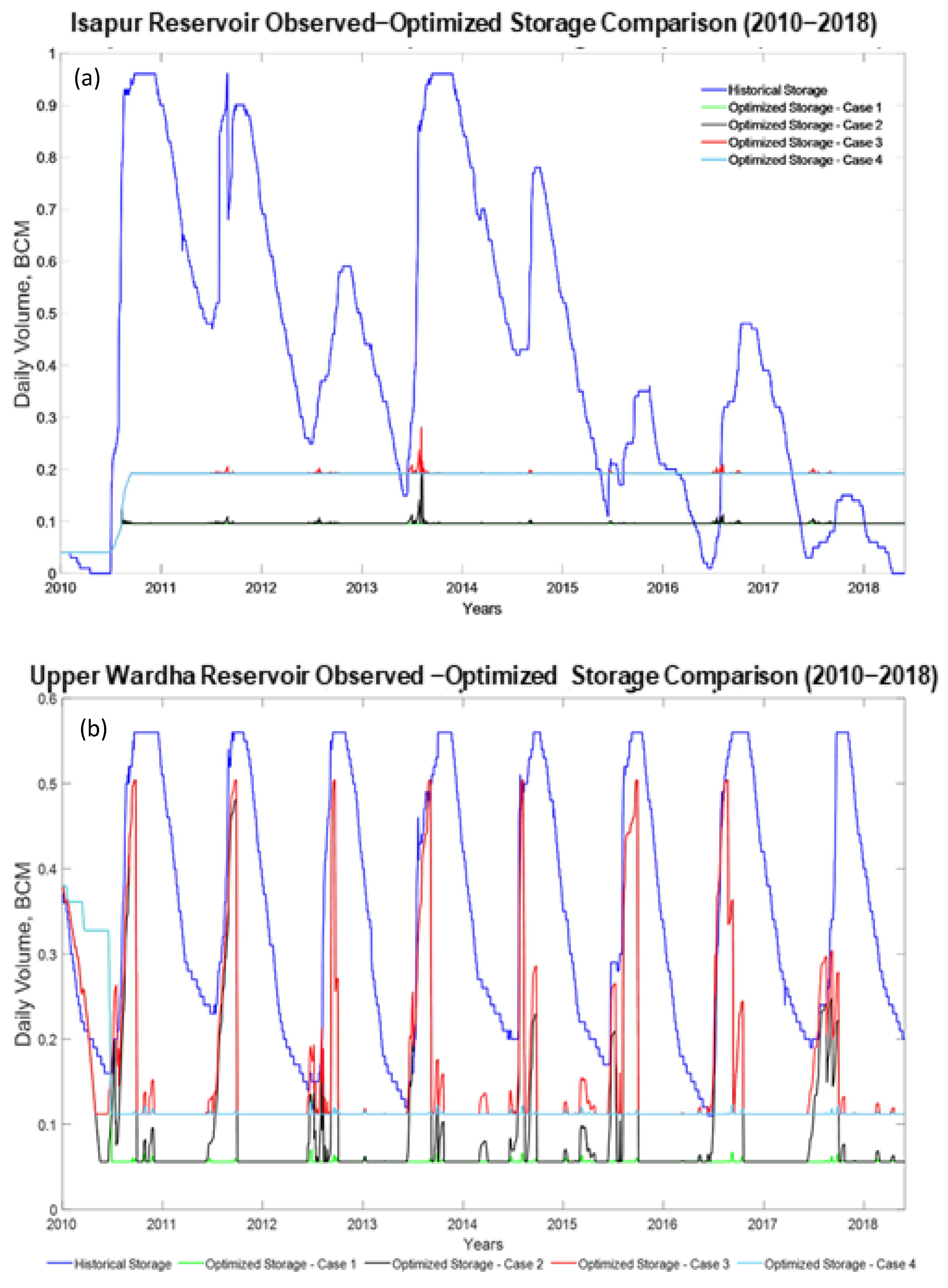
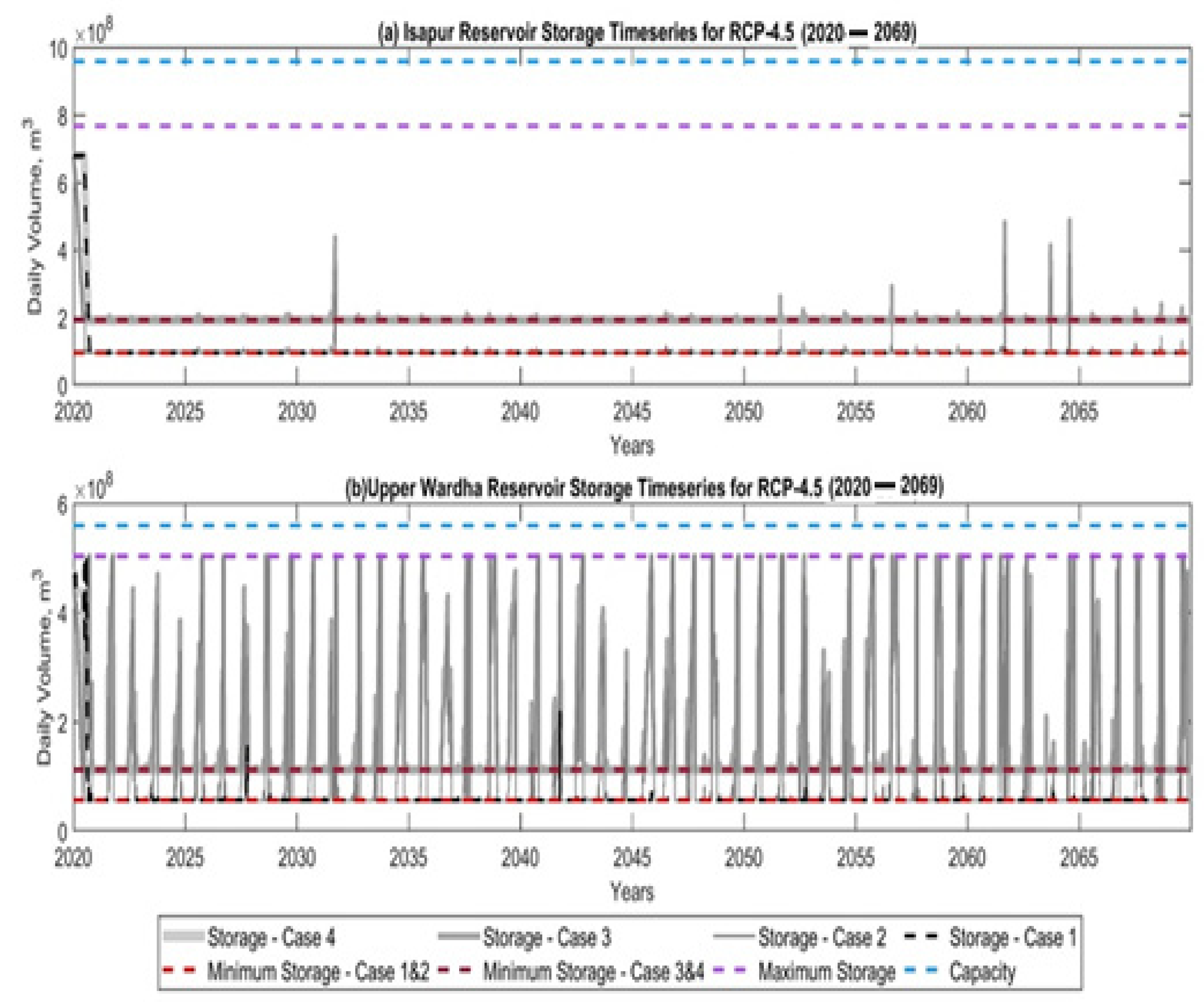
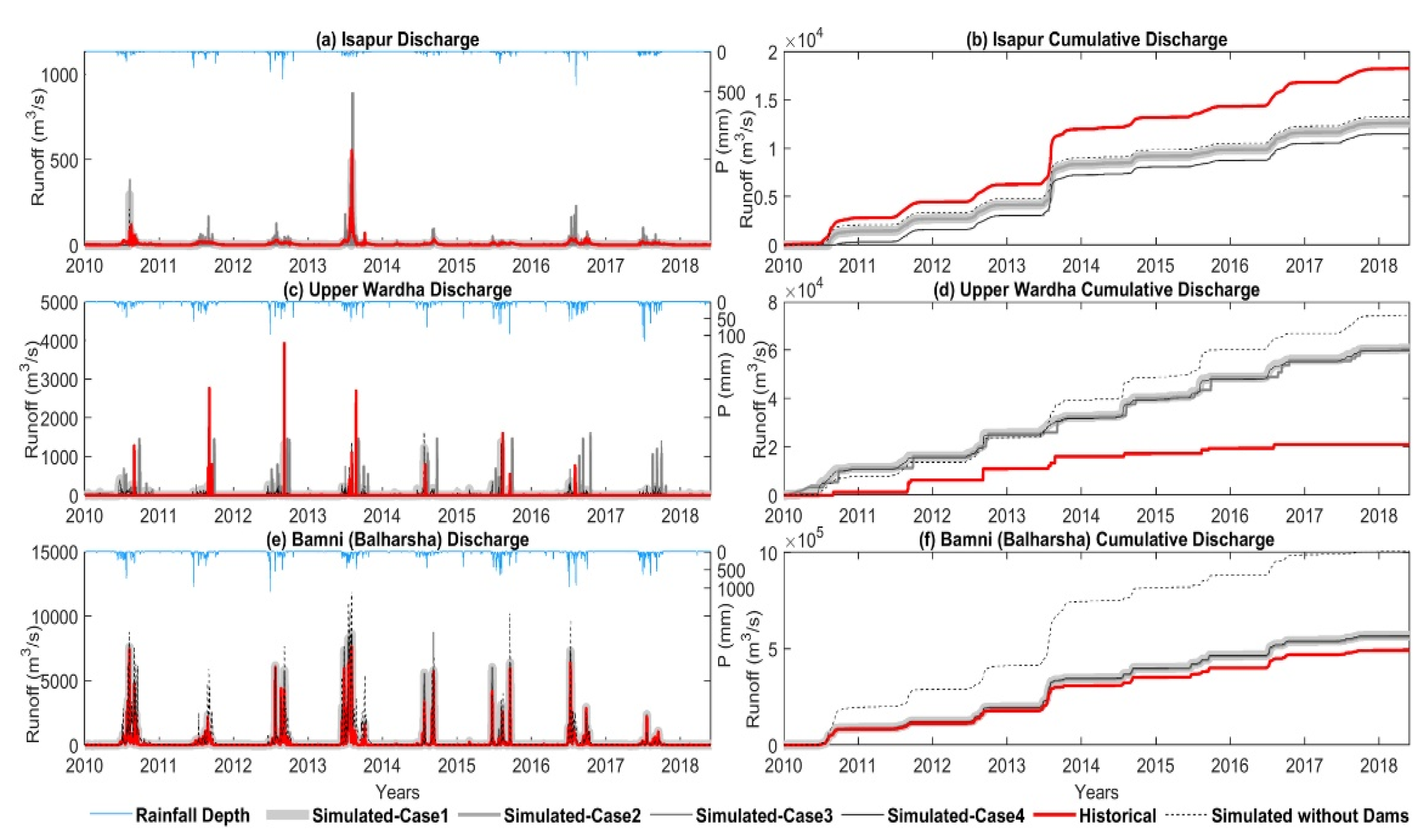
At the beginning of this study, the hydrologic basin model was developed using the HEC-geoHMS and Arc-Hydro tools in ArcGIS. These tools were used to delineate the basin model and to calculate the basin and stream parameters. They were also used to process the land cover, soil cover, and precipitation gridded maps, which were converted into data storage system (DSS) files.

Figure 8 illustrates the entire flow chart of the integration process of the analyses. The basin model generated from HEC-geoHMS needed to be separated into three sub-watersheds. Two of the sub-watersheds were constructed upstream of the Isapur and the Upper Wardha Reservoirs. After simulating these upstream sub-watersheds, the outflow data were saved in DSS files. These outflow data were used as reservoir inflow time-series parameters by the GAMS models. The data from DSS files were converted into CSV files using JavaScript, which were transformed in Python to use them as inflow parameters in GAMS (see Figure 8b). GAMS was used to optimize the water supply, and to provide the reservoir outflow and storage time-series data as the output. These outflow data were then converted to a time-series flow variable of the DSS file of the third hydrologic model, which was constructed for the downstream part of the watershed. Subsequently, the HEC-HMS model conducted the final step of the simulation by providing the outflow data of downstream sub-watersheds.

3. Results

Figure 9 demonstrates the storage time-series patterns of the reservoirs of 2010 to 2018 with the optimization theory applied. This simulation of the historical time period helps to identify the difference between the optimized simulation cases and the historical discharge pattern. In these curves, the historical patterns do not follow any specific constraint for reservoir storage. The storage shift varied from 4% of the capacity to 100% of the capacity according to the requirement upstream of the Isapur Dam. By comparison, storage fluctuated from 25% to 100% of the capacity in the Upper Wardha Dam for the historical scenario. For most of the time, the storage volumes for simulated flows were forced to remain close to the minimum storage limit (10% of the capacity for case 1 and case 2, and 20% of the capacity for case 3 and case 4) due to less availability of water.

Figure 10 and Figure 11 elaborate the predicted Upper Wardha Reservoir storage time-series for different constraint cases for RCP-4.5 (Figure 10) and RCP-8.5 (Figure 11) scenarios for 2020 to 2069.

Figure 12 shows comparisons between the observed and optimized discharge time-series, and comparisons of observed and optimized cumulative discharge time-series. Here, the red line indicates the historical time-series, and the grey lines with different thicknesses indicate simulated discharges for different constraint cases. However, Figure 13 illustrates hydrographs and rainfall hyetographs at four different stations.

Figure 14 illustrates the comparison between cumulative discharge and cumulative downstream demand at four different stations of the watershed.

4. Discussion

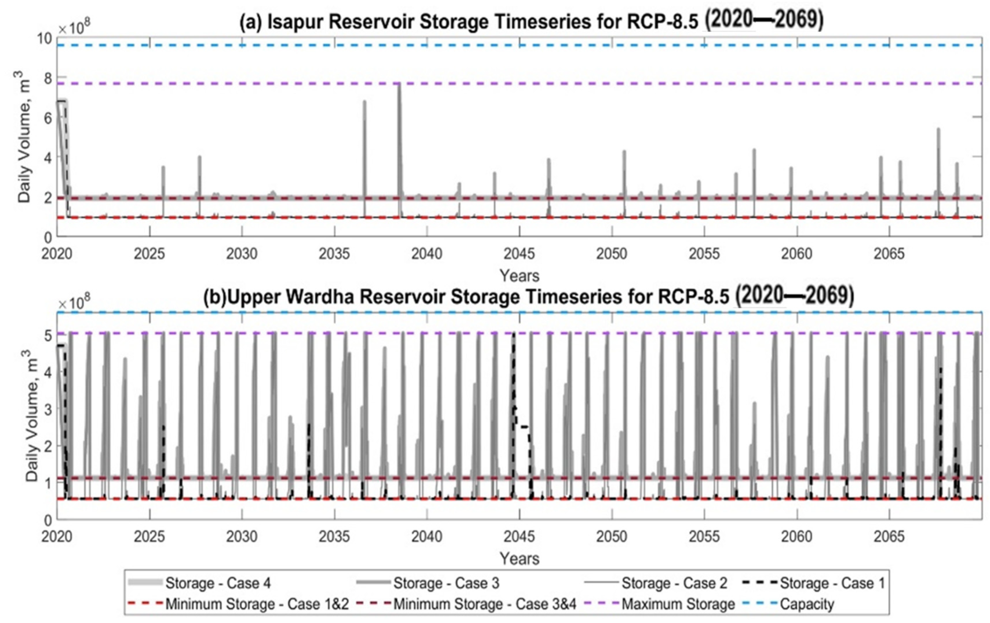
4.1. Reservoir Storage Pattern

The reservoir storage time-series curves in Figure 10 and Figure 11 provide information about the storage constraints and their fluctuations with time due to predicted precipitation for RCP-4.5 and RCP-8.5 scenarios. The observed storage curve of the Isapur Dam for the historical period (2010–2018) in Figure 9 illustrates that the Isapur Reservoir stored a larger volume of water than required.

Figure 9 shows a gradual degradation of the storage pattern from 2010 to 2018. For constraint combination cases one and four, the simulated storage levels of the Isapur Dam were kept at the minimum level during the entire 50-year period, which assists in maximizing the releases from the limited inflows. However, the Upper Wardha Reservoir storage followed a harmonic pattern during the entire timeline. Because case 2 and case 3 consider the net water demand as the maximum limit of reservoir releases, it reduces the releases during precipitation, which causes increased storage levels of water in both of the reservoirs due to rainfall.

The historical storage pattern illustrates that the storage fluctuated from 4% of the capacity to 100% of the capacity. This occurred because of inefficient reservoir operation, biased local politics, inequality of privileges, and favoritism. The simulated models in this study targeted the storage of a sufficient amounts of water for indigenous people and release of excess water to reduce downstream damage. Because this study represents a pilot project, further analysis of the allowable storage range for reservoir operations is required in the future.

4.2. Downstream Water Allocation Analysis

Figure 12 incorporates hydrographs and cumulative hydrographs at the dam release points and the most downstream station (Bamni–Balharsha) of the basin. It considers three different scenarios of reservoir operations, namely: observed discharge, simulation considering a no-reservoir scenario, and simulation considering maximization of the reservoir releases for four different constraint cases.

For the Isapur Reservoir, the observed hydrograph shows some shallow peaks during rainfall, which is an indication of very low releases from this dam (see Figure 12a). The cumulative discharge curve for the Isapur Dam in Figure 12b illustrates that the estimated cumulative discharge is larger than the cumulative discharges for the simulated cases. This can occur due to the timing of gate openings. A storm having a long duration may cause a massive discharge downstream. However, these discharges do not effectively contribute to the downstream locations. During a storm, the demands for both the downstream and upstream areas are met from direct rainfall. As a consequence, these areas cannot utilize the excess flow from upstream. Thus, these unoptimized discharges cause no improvement, except increasing the cumulative discharge records.

For the Upper Wardha Reservoir, the reverse outcome for historical and no-reservoir scenarios indicates that there would be an increased flow downstream for the no-reservoir scenario. For both of the reservoirs, the cumulative discharges for optimized releases indicate that the water supply can be significantly improved if the optimization were utilized for reservoir operation. The combination of the reservoir releases and rainfall intensity can meet the water demand in the downstream portion of the watershed. A comparison of the cumulative historical and simulated discharge curves at the most downstream point of the Wardha Watershed (Bamni-Balharsha) shows that the simulated models can deliver about 19% more water than the historical discharge. The application of optimization theory to the operation of the Upper Wardha Dam can increase the supply of water by about 66% compared to the historical discharge at the Ghugus downstream station (before merging with the stream from the Isapur Dam). Although the simulated releases from the Isapur Dam do not show any increase in the water supply compared to the historical discharge downstream, the appropriate timing of the release gate operation using this optimization model can utilize the maximum use of the discharge for irrigation purposes and reduce the loss of excess water.

Figure 13 demonstrates the reservoir future release–demand comparison for simulation case 3 due to the RCP-8.5 scenario. The remainder of the comparison graphs for other simulation cases due to RCP-4.5 and RCP-8.5 are provided in the Supplementary section. Figure 14 reveals the cumulative release–demand patterns for the same scenario (case three and RCP-8.5). These patterns illustrate that, for all the simulation cases and scenarios, at the downstream stations of the Isapur Dam, the simulated cumulative discharges cannot meet the demand curve, although the performance is better than that of the historical observed cases. The downstream stations of the Upper Wardha Dam show more acceptable discharges compared to the demand curve.

The analysis indicates that, before implementing a project having a large budget, the authorities should utilize the optimization in reservoir operation to address the issue of water scarcity. Even if the water demand increases, the model can deliver an amplified volume of water towards the downstream region of the reservoirs more efficiently than the observed pattern. To operate the optimized reservoir release in real life, the operators should consider a number of cases to schedule the reservoir gate operations, including the seasonal water demand downstream, short- and long-term rainfall predictions for the entire watershed, and existing reservoir storages. Although this study considered the minimum storage of the reservoirs as 10% and 20% of the reservoir capacities, the lower limit of the storage can be estimated according to the demand ratio of the areas upstream and downstream of the reservoirs. Moreover, the storage should be maintained close to the lower limit when there is no possibility of rainfall in the downstream areas.

5. Recommendations

The analysis considered the Norwegian Earth System Model 1 (NorSEM) for RCP-4.5, and the Community Climate System Model (CCSM4) for RCP-8.5 rainfall prediction. Because the RCP predicted data and the historical rainfall data are available for the period from 2006 to 2020, these datasets needed to be bias-corrected using the historical rainfall dataset of this period, and predicted more accurately for the 21st century.

A study of groundwater hydrology of the surrounding basin would increase the accuracy of the model. However, due to the lack of accessible groundwater data, this additional study could not be conducted. Moreover, in this research, groundwater extraction was not considered in creating the limiting release constraint of the optimization model.

The hydrologic functionalities of the entire Wardha Watershed are dependent on the Isapur and Upper Wardha Dams. To build the hydrologic model of this basin, the availability of data relating to the reservoir time-series discharge, storage, and stages was important. Although the storage and stage data were accessible through the India-WRIS data portal, the reservoir outflow data were not available. To create a more robust hydrologic model, managing historical time-series release data may be a better option.

Evapotranspiration is an important basin parameter for defining a sub-basin of a hydrologic model. This study was only able to collect evapotranspiration time-series data for a period of 2.5 years. A longer time-series of data would be helpful to more accurately estimate evapotranspiration.

The basin model was used to analyze 20 years of historical data and predict 50 years of discharges throughout the basin. The hydrologic parameters were considered to be constant for this 70-year timeline. The changing pattern of these parameters with time may be estimated and utilized in the model to ensure a better prediction of the hydrographs.

The optimized reservoir operation may cause a change in water quality, which should also be analyzed for future predictions. The analysis of biodiversity is one of the techniques that may be used to assess the water quality of the surrounding water bodies.

This study did not perform any cost-benefit analysis or maximization of agricultural profit. Profit analysis requires the identification of the existing cost and price of each crop. This analysis can assist in understanding the most profitable cropping pattern of the Umarkhed region.

6. Summary

This study demonstrates that an efficient water supply plan requires effective reservoir optimization, including a suitable water supply system. The integrated model in this study simulated a greater supply of water than the historical discharge. Moreover, the optimized simulation approaches were able to satisfy the downstream demands in most of the watershed. The optimized releases of the Upper Wardha Reservoir were better able to satisfy the downstream demand than those of the Isapur Reservoir. Umarkhed Taluka is situated around 31 kms downstream of the Isapur Reservoir, where the optimization model cannot completely satisfy the water demand. Among the four cases of the optimization models, the second and third scenarios considered downstream water demand during the reservoir operation. This optimization technique stores excess inflows when the downstream net water demand decreases during precipitation. The other two scenarios were built in a manner to benefit the areas upstream of the reservoirs by allowing reservoir release only when there are inflows from upstream areas. As a consequence, the storage patterns provide more fluctuations in case 2 and case 3. Because the downstream areas of Umarkhed receive more water compared to the amount of water demanded, a water storage system needs to be utilized. According to the developed model, the downstream sub-basin outlets, including Hivra, Ghugus, and Bamni, receive more water than is demanded. A plausible solution to the problem of water scarcity in Umarkhed can be introduced by storing an effective amount of water in the downstream regions near the outlet of the Wardha sub-basin, and building a system to deliver water upstream to Umarkhed. In order to utilize an effective optimized reservoir operation in the actual scenario, the operators need to consider a number of cases that include the short- and long-term rainfall forecasts, present and future water demand, and the existing storage of the reservoirs.

References

1. Jain, S.K.; Kumar, V. Trend analysis of rainfall and temperature data for India. Curr. Sci. 2012, 102, 37–49. [Google Scholar]
2. Bodh, P.C. Farmers’ Suicides in India: A Policy Malignancy; Taylor & Francis: Abingdon, UK, 2019. [Google Scholar]
3. Gawande, S. GSG College Meeting with CU—Boulder MENV. January 2020. Available online: https://www.colorado.edu/menv/2020/02/04/menv-team-collaborates-gopikabai-sitaram-gawande-college-and-student-and-education (accessed on 5 June 2021).
4. Naga, S.P.; Venkata, R.K.; Shashi, M. Intra- and interannual streamflow variations of Wardha watershed under changing climate. ISH J. Hydraul. Eng. 2020, 26, 197–208. [Google Scholar] [CrossRef]
5. Gujja, B.; Dalai, S.; Shaik, H.; Goud, V. Adapting to climate change in the Godavari River basin of India by restoring traditional water storage systems. Clim. Dev. 2009, 1, 229–240. [Google Scholar] [CrossRef]
6. Garg, V.; Dhumal, I.R.; Nikam, B.R.; Thakur, P.K.; Aggarwal, S.P.; Srivastav, S.K.; Kumar, S. Water resources assessment of Godavari river basin, India. In Proceedings of the ACRS Conference 2016, Colombo, Sri Lanka, 17–21 October 2016; Volume 17. [Google Scholar]
7. Tupe, S.; Joshi, V. Trends in agriculture of Yavatmal Maharashtra (India): District Level Analysis. Agro Econ. 2019, 6, 87–92. [Google Scholar]
8. Sandrp. Godavari Basin in Maharashtra: A Profile. 2017. Available online: https://sandrp.in/2017/03/08/godavari-basin-in-maharashtra-a-profile (accessed on 15 November 2021).
9. Gosain, A.K.; Rao, S.; Basuray, D. Climate change impact assessment on hydrology of Indian river basins. Curr. Sci. 2006, 90, 346–353. [Google Scholar]
10. Das, J.; Umamahesh, N.V. Downscaling Monsoon Rainfall over River Godavari Basin under Different Climate-Change Scenarios. Water Resour. Manag. 2016, 30, 5575–5587. [Google Scholar] [CrossRef]
11. Feldman, A.D. Hydrologic Modeling System HEC-HMS Technical Reference Manual [Computer Software Technical Reference Manual]; U.S. Army Corps of Engineers: Washington, DC, USA, 2000. [Google Scholar]
12. Fleming, M.J.; Doan, J.H. HEC-geoHMS Geospatial Hydrologic Modeling Extension [Computer Program Documentation]; U.S. Army Corps of Engineers: Washington, DC, USA, 2009. [Google Scholar]
13. Roy, P.S.; Meiyappan, P.; Joshi, P.K.; Kale, M.P.; Srivastav, V.K.; Srivastava, S.K.; Krishnamurthy, Y.V.N. Decadal Land Use and Land Cover Classifications across India, 1985, 1995, 2005; ORNL DAAC: Oak Ridge, TN, USA, 2016. [Google Scholar]
14. Brouwer, C.; Heibloem, M. Irrigation Water Management: Irrigation Water Needs (Training Manual No. 3); FAO: Rome, Italy, 1986. [Google Scholar]
15. Worldometer. Water Use in India. 2017. Available online: https://www.worldometers.info/water/india-water (accessed on 15 November 2021).
16. Roy, D.; Begam, S.; Ghosh, S.; Jana, S. Calibration and validation of HEC-HMS model for a river basin in eastern India. ARPN J. Eng. Appl. Sci. 2013, 8, 40–56. [Google Scholar]
17. Loucks, D.P.; Beek, E.V. Water Resources Systems Planning and Management; Elsevier: Amsterdam, The Netherlands, 2017. [Google Scholar] [CrossRef]
18. Kallrath, J. Modeling Languages in Mathematical Optimization; Springer: Berlin/Heidelberg, Germany, 2013; Available online: https://link.springer.com/book/10.1007/978-1-4613-0215-5 (accessed on 15 November 2021).
Figure 1. Location of the Godavari River basin and the Wardha sub-basin in India. Both of the figures indicate the location of the Wardha sub-basin (red region) within (a) India and the (b) Godavari River basin.
Water 14 00114 g001
Figure 2. (a) Digital Elevation Model (DEM): the reddish border indicates the most upstream parts of the sub-basin where the blueish color defines the downstream part; (b) land use and land cover classification (2005): mostly agricultural land; (c) soil type map of the Wardha Watershed where a large portion of soil is Chromic Vertisols; (dg) illustrate NDVI during different months of the water year 2021 ((d) October, (e) January, (f) April, and (g) July).
Water 14 00114 g002
Figure 3. (a) Gridded precipitation pattern (sample date: 1 October 2001), and (b) grid coordinate transformation using interpolation for predicted rainfall time-series data. The black grids represent the predicted RCP rainfall grid location, and the red grids represent the modified grid position that overlaps with the historical rainfall grids.
Water 14 00114 g003
Figure 4. (a) Estimated average daily evapotranspiration of the Yavatmal District. Here, crops of the Rabi season (which starts in October), namely, wheat, chickpeas, etc., require additional water in September and October according to the calculation of daily evaporation. (b) Different water use patterns in India [15].
Water 14 00114 g004
Figure 5. (a) Contributing area of the Wardha Watershed: the yellow triangles represent the location of the reservoirs, and the blue and magenta outlines indicate the upstream watersheds of the Upper Wardha and the Isapur dams, respectively; and (b) schematic representation of the basin model in HEC-HMS, where green, blue, and red circles represent the locations of the sub-basin centers, junctions, and dams, respectively.
Water 14 00114 g005
Figure 6. Comparison of calibrated-observed and validated–observed hydrographs at Kanhargaon and Bamni (Balharsha) stream gauge stations for observed rainfall hyetographs of their upstream sub-basins.
Water 14 00114 g006
Figure 7. Illustration of mass balance of a reservoir.
Water 14 00114 g007
Figure 8. (a) Flow of the integrated hydrologic and optimization modeling method, and (b) stages of the optimization simulation model.
Water 14 00114 g008
Figure 9. Comparison of observed–optimized storage for 2010 to 2018 of (a) the Isapur Reservoir, and (b) the Upper Wardha Reservoir.
Water 14 00114 g009
Figure 10. Optimized storage for RCP-4.5 scenario for 2020 to 2069 of (a) the Isapur Reservoir and (b) the Upper Wardha Reservoir.
Water 14 00114 g010
Figure 11. Optimized storage for RCP-8.5 scenario for 2020 to 2069 of (a) the Isapur Reservoir and (b) the Upper Wardha Reservoir.
Water 14 00114 g011
Figure 12. Comparison of observed and optimized discharge/cumulative discharge for different stations—(a) Isapur Reservoir releases, (b) Isapur Reservoir cumulative releases, (c) Upper Wardha Reservoir releases, (d) Upper Wardha Reservoir cumulative releases, (e) Bamni (Balharsha) discharge, and (f) Bamni (Balharsha) cumulative discharge.
Water 14 00114 g012
Figure 13. Hydrographs and rainfall hyetographs at four different stream gauge stations, namely, (a) Isapur Reservoir, (b) Upper Wardha Reservoir, (c) Station J17249 (downstream station of Umarkhed Taluka), and (d) Bamni-Balharsha (outlet of the watershed), for RCP-8.5 climate change scenario and case 3 constraint combination of the optimization model.
Water 14 00114 g013
Figure 14. Cumulative hydrographs at four different stream gauge stations, namely, (a) Isapur Reservoir, (b) Upper Wardha Reservoir, (c) Station J17249 (immediate downstream station of Umarkhed Taluka), and (d) Bamni-Balharsha (outlet of the watershed), for RCP-8.5 climate change scenario and case 3 constraint combination of the optimization model.
Water 14 00114 g014