1. Introduction
High suspended solids and phosphorus concentrations affect the water quality and cause eutrophication of rivers and lakes [
1]. This hampers the achievement of the objectives of the European Water Framework Directive [
2]. The member states of the EU must ensure that a good chemical and ecological status is reached in all water bodies. To achieve this aim, necessary measures must be implemented. The monitoring of substances in rivers is important to gain knowledge about the current emission situation (concentrations and loads) and to develop appropriate measures to reduce the emissions into water bodies.
The calculated river loads help to verify the amount of modeled inputs and to identify their temporal and spatial variability. For an accurate river load calculation, concentration and discharge data representing the hydrological conditions completely is needed. In Germany, the hydrographs of the discharge are mostly available as hourly mean values. Concentrations are usually the result of grab samples taken on a calendar-based schedule. The intervals usually vary from weekly to monthly sampling. Several studies show that this type of sampling is not adequate to represent the actual load in the river [
3,
4,
5]. This is partly due to the fact that grab sampling is not suitable for capturing short-duration peaks in sediment or phosphorus concentrations [
5]. Horowitz [
4] stated that at least 80–85% of a river’s discharge should be covered by the sampling and that additionally as many high flows as possible need to be sampled to realistically capture the annual load. For calendar-based sampling strategies, the probability to record mainly mean flow conditions in the river is very high. Thus, high and low flow conditions are likely to be underrepresented, which means that they are not considered in the load calculations. Particulate-bound substances such as phosphorus are mobilized at high flow rates and are transported within the water body. Especially for substances with a high solid affinity, randomly distributed grab samples are not suitable [
6]. Composite samples taken over a period of several days help to overcome the described problems and to determine the loads transported in rivers more representatively [
3].
In this research, large-volume samplers (LVSs) have been used for river monitoring. They allow to take composite samples over a variable period of time [
6,
7,
8]. With LVSs, a quasi-continuous sampling is possible, allowing long observation periods at reasonable costs and making it easy to catch a considerable share of the discharge volume. Additionally, the resulting amount of sediment in the LVS is large enough for further analyses like grainsize distribution, grainsize specific organic content and substance loading. LVS concept has been applied in many studies to monitoring in urban sewer systems [
8,
9], wastewater treatment plants [
10] and rivers [
7,
11]. It has been proven that it is very robust and ideally suited to generate representative average concentrations for load calculations, e.g., annual river loads.
The LVSs were used in two different sampling modes with a focus on the calculation of annual river loads of suspended solids and phosphorus in the river. Both parameters are known to be the cause for not achieving a good ecological status in surface waters in the respected region. The results of this study have been used by Allion et al. [
12] who separated emissions of different pathways (agriculture, sewer systems) in the catchment and thus verify modeled erosion inputs into the river.
The overall aim of this article is to develop an approach suitable to determine the sediment and phosphorus load transported in rivers. The results of two sampling strategies of the LVS (quasi-continuous vs. event-based) are evaluated. The aims are to (1) quantify the solids and phosphorus load in the Kraichbach river with the two strategies and (2) to discuss the advantages and disadvantages of the strategies. Based on the result, (3) a recommendation for further monitoring strategies should be made.
2. Materials and Methods
2.1. Study Area Characteristics
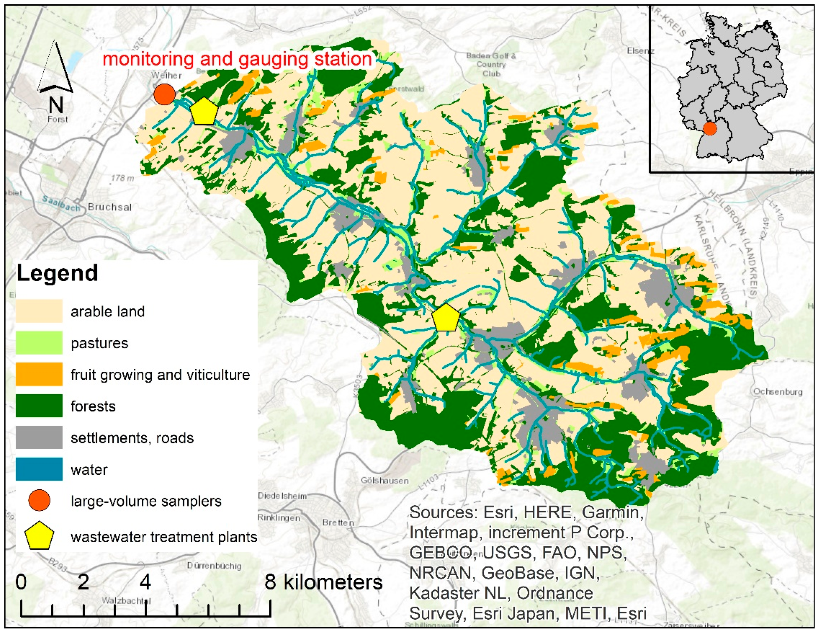
The Kraichbach river, a tributary of the Rhine, is located in the north-west of Baden-Wuerttemberg (Germany) and has a length of about 55 km. The monitoring station of this study is located next to the gauging station ‘Ubstadt’ at the transition zone of the loess dominated Kraichgau and the Upper Rhine Valley. The catchment area at this location is 160 km² and is characterized by a hilly landscape with agriculture and loess soils. Both land use and soil properties make the slopes in the catchment prone to erosion. At 52%, the major part of the catchment area is used for agriculture, 6% of the area is covered with grassland, vineyards account for 4%, forests for about 30% and settlement areas for about 8% (
Figure 1). The annual precipitation in the area is 700 mm a
−1 [
11].
At the monitoring station, the river has a width of about 4.5 m and a depth of 0.58 m at its deepest point during mean flow conditions. The official long-term (30 years) discharge indicators for the gauging station are a mean flow rate (MQ) of 1.1 m
3 s
−1 and a mean low flow rate (MNQ) of 0.614 m
3 s
−1 [
13]. The flow rate of a flood event with a probability to occur every two years (HQ2) is 7.79 m
3 s
−1 [
14].
2.2. Large-Volume Sampler
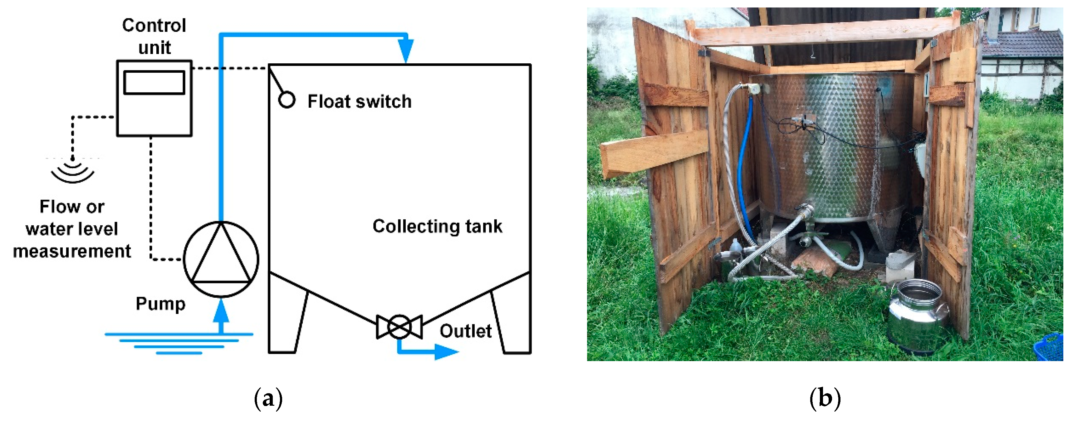
Figure 2 shows a scheme and a photo of the LVS used in this study. The samples from the river are collected in a 1000 L stainless steel tank that is set up in an enclosure. A control unit translates the water level signal of the gauging station ‘Ubstadt’ into a discharge by a polynomial function and controls the discharge-proportional sampling. The control unit is programmed to pump a 10 L subsample of the river into the tank, after a specific discharge volume has been exceeded. The pump is installed almost in the middle of the cross section of the river so that no sediment is stirred up and the influences of bank and riverbed are minimized. The discharge-proportional composite samples are collected over two to four weeks. The control unit saves the settings, the water level and the discharge as well as information about the status of the pump in a log file by minute. To prevent the tank from overflowing, a float switch is installed at the top of the tank. After the tank has been filled, the samples are taken after a settling period of three to four days. The supernatant sample is collected in a 2 L bottle, the solid sample in a 15 L stainless steel can after draining the supernatant water back to the river downstream of the pumps. Both samples are brought to the laboratory immediately after sampling.
In this study, two LVSs have been used with the same set up. The pumps of both LVSs are installed at the same riverbank side, but with enough distance to exclude the disturbance of each other. The two LVSs are used to compare the quasi-continuous (LVS1) and event-based (LVS2) sampling strategies.
2.3. Sampling Strategy
At the Kraichbach river, the first large-volume sampler (LVS1) was installed in 2017 and is still in use. The LVS1 is used with a quasi-continuous sampling strategy and collects long-term volume-proportional composite samples. The LVS1 monitoring results are supposed to be used for annual river load calculation with a rating curve. As this method is based on constant sampled discharge volumes, the aim of this monitoring strategy is to sample a constant discharge volume as exactly as possible. Using minutely discharge data is helpful to detect the start and stop of the pump as well as the passed discharge volume at the LVS very accurately. Therefore, it can be assumed that a full tank represents a discharge volume that does not vary too much among the samples.
In 2020, a second sampler (LVS2) was installed. It is operated with an event-based sampling strategy, which means that different flow conditions, such as high flows after rainfall events or dry weather periods, are sampled specifically. The setup of the LVS2 is the same as that of the LVS1, only the parameters pumping interval and start of sampling (threshold value) are adapted. The pumping interval is set to a higher interval to have a sufficient amount of sediment in the tank. For rainfall events, the start value was set to a flow of 1.1 m3 s−1 at the control unit to separate the event from low flow conditions.
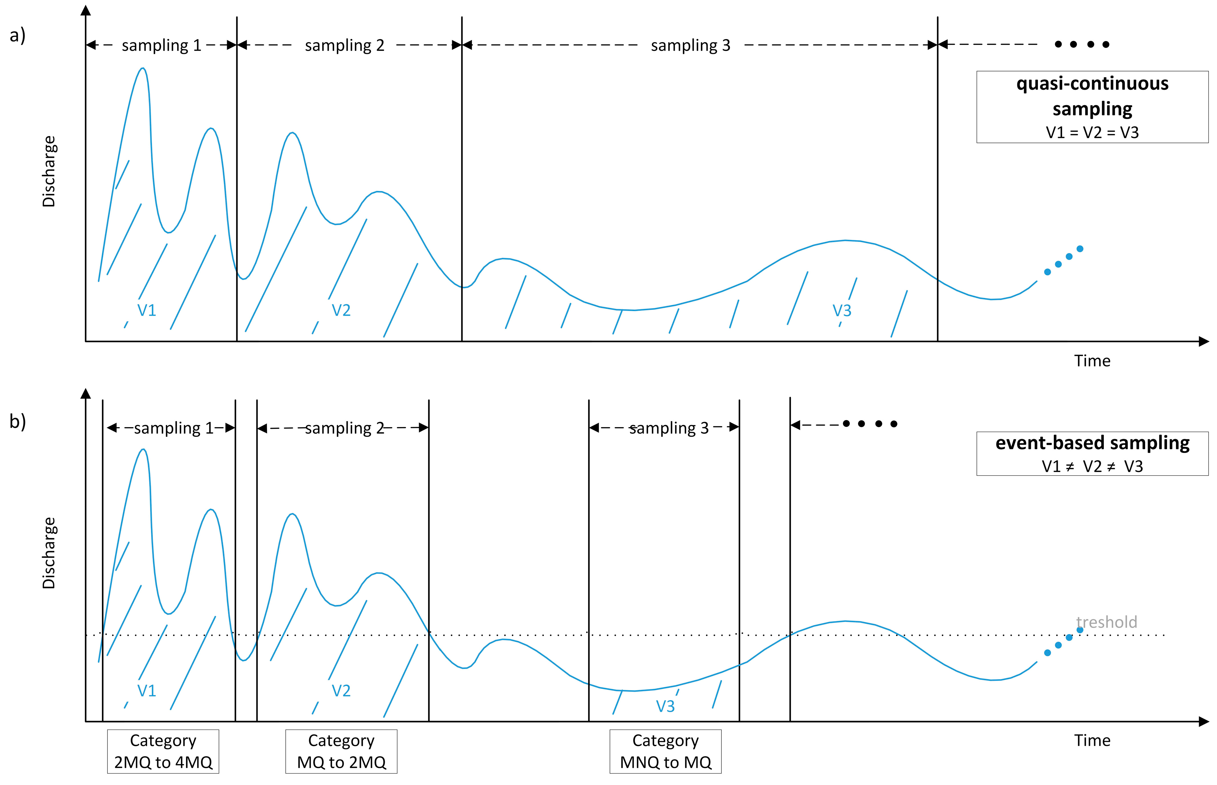
Both sampling strategies are shown schematically in
Figure 3. With the quasi-continuous sampling strategy, each sample covers the same discharge volume (V). For the event-based sampling, the sampled discharge volume is different for each sample, because high discharge sampling starts as soon as the discharge exceeds the threshold value and stops automatically when the discharge falls below this threshold again. Low and mean discharge sampling are started and stopped manually. The sampled volume depends on how long these conditions last in the river.
2.4. Analytical Methods
All samples of the LVSs were analyzed in the same laboratory. The supernatant water was analyzed for total suspended solids (TSS in mg L−1, DIN 38409-H2) and orthophosphate-phosphorus concentration (PO4-P in mg L−1, DIN 38405 D11-4). The sediment samples were homogenized, sieved (standardized 63 µm sieve) and dried at 105°C to determine the total dry mass (MSed in mg, DIN 38409-H1). The loss-on-ignition (LoI in %, heated to 550 °C for 120 min, DIN38409-H2) as well as the total phosphorus content (Ptot in mg/kg, DIN 38405 D11-4 after perchloric acid digestion) were analyzed.
2.5. Data Analysis
In order for sampling to correspond to discharge as closely as possible and thus guarantee the discharge-proportional sampling and a constant discharge volume (in the case of LVS1), the control unit was driven by minutely discharge data, which means start and end time, as well as exceeding thresholds can be defined quite exactly. However, these data are only available during the sampling periods, whereas hourly discharge data at the nearby gauging station ‘Ubstadt’ are freely available over years and are used, discussed and evaluated in many projects and by local authorities. For this reason, and also to be able to apply the monitoring results to long-term discharge data, all data analysis refers to hourly discharge data, measured by the official gauging station ‘Ubstadt’ during the sampling periods. Minutely discharge data are not analyzed further, but were used to define the exact start and end of a sampling period as well as the sampled discharge volume.
2.5.1. Calculation of Mean River Concentrations
The data from the laboratory analysis are used to calculate a mean concentration in the tank. As river water was pumped into the tank proportional to the discharge of the river, the concentration in the tank represents the mean river concentration during the sampling period. Nickel and Fuchs [
15] use the term ‘Event Mean Concentration’ (EMC) for their evaluations, as they investigated discharge peaks resulting from rainfall events in their study. As the quasi-continuous sampling strategy in our study does not investigate single hydrological events, but periods with an arbitrary discharge curve, the term ‘Event Mean Concentration’ is misleading. Therefore, the term ‘Sampling Period Mean Concentrations’ (SPMC) is used instead, although the calculations of the SPMC and the EMC do not differ. For the event-based sampling strategy of the LVS2, the term EMC by Nickel and Fuchs [
15] is kept, because here different hydrological situations such as low flow conditions, mean and high flow events are investigated specifically.
Quasi-continuous sampling
The SPMC of suspended solids of the LVS1 (SPMC
LVS1,SS) were calculated as shown in Equation (1). The overall concentration SPMC
LVS1,SS is determined by transferring the dry mass of the sediment (M
Sed) settled in the tank into a concentration using the sample volume in the tank (V
LVS1) and adding the concentration of fine suspended solids in the supernatant water C
TSS. The phosphorus concentrations SPMC
LVS1,P (Equation (2)) were determined in the same way. Here, the total P content in the settled sample is considered (P
tot).
Event-based sampling
Different events (flow conditions) are sampled with the LVS2. After an event, the LVS2 is not always filled completely which means, that the sampled discharge volume is different for all investigated samples. EMCs (EMC
LVS2,SS and EMC
LVS2,P) are calculated in the same way as SPMC for the LVS1 samples (Equations (3) and (4)).
The sampled events and derived EMCs are grouped concerning their flow conditions according to official long-term discharge indicators into low discharge (MNQ), mean discharge (MQ), and discharge higher than mean flow (>MQ) according to the Qmax of the event. For each discharge-condition category, median concentrations of suspended solids and phosphorus (CLVS2,cat,i) out of the single EMCs were calculated.
2.5.2. Calculation of Annual River Loads
For the calculation of annual river loads, two different methods were applied. The first approach is based on the concentration-discharge regression and the second approach is a discharge-corrected standard method [
3]. Both have in common that the mean concentration shows a high correlation with the maximum discharge during the sampling period.
For the calculation of annual loads, freely available hourly discharge data of the gauging station ‘Ubstadt’ are used.
Quasi-continuous sampling
To calculate annual river loads for the LVS1 using the quasi-continuous sampling strategy, a rating curve that derives the SPMC depending on the maximum discharge during the sampled period was used according to Wagner [
11]. The concentration-discharge-regression is limited by the highest measured concentration and the highest sampled discharge. The rating curve was applied to long-term discharge data (2003–2020) in order to calculate annual suspended solids and phosphorus loads. As the rating curve is based on measurements referred to a constant cumulated discharge volume, the concentrations given by the curve are only useable if applied to the same water volume. For this purpose, the hourly discharge measurements of the gauging station ’Ubstadt’ from 2003–2020 were divided into equal segments with the same cumulated discharge volume. For each segment, the maximum hourly discharge (Q
max) was determined and corresponding to the rating curve a mean concentration was identified. For segments with a Q
max higher than the validity of the rating curve, highest valid Q
max of the rating curve was assumed. By multiplying the mean concentration with the volume of the segments, sampling period loads (load
LVS1) were calculated and summed up to annual river loads (Equation (5)).
Event-based sampling
With the LVS2 the resulting volume of the sample in the tank as well as the sampled discharge volume differ among the samples. Therefore, it is not possible to divide a discharge curve into segments and apply a rating curve, as a criterion for cutting the discharge curve (such as a constant discharge volume in the case of the quasi-continuous sampling strategy) would be needed. For this reason, to calculate annual river loads (load
LVS2) with the event-based sampling strategy of the LVS2, hourly discharge values were grouped in the categories of low, mean and high flow conditions (V
cat,i). The volume V
cat,i of the categories was then multiplied with the median concentration (C
LVS2,cat,i) (Equation (6)). For each year, the loads of the categories were summed up to the annual river load
4. Discussion
Many studies show that grab samples are not suitable to capture the actual load in the river [
3,
4,
5,
16,
17,
18,
19]. With weekly or monthly sampling strategies, it is likely to miss the discharge peaks. However, especially for particulate-transported substances, these peaks are periods with high substance concentrations and the greatest contribution to the annual load. For grab samples, the measured concentrations are applied to a long-time period (via discharge), although the concentration does not represent the conditions of the periods before and after the sampling [
19].
To confirm this statement, besides the composite samples during each LVS sampling period, a grab sample at the gauging station ‘Ubstadt’ was collected and analyzed for total phosphorus concentration and total suspended solids (
Table S7). The measured concentrations of the grab samples per year were used to calculate the river load with a discharge-corrected standard method [
3] (
Table 4 and
Table S8). The results confirm that river loads calculated from grab samples taken approximately once a month are not reliable, as they depend too much on what flow conditions are actually sampled. In 2020, one sample of sixteen taken during high flow (4.19 m
3 s
−1) is responsible for an extremely high suspended solid load of around 4800 t per year. If this sample is not considered, the resulting solid load drops to 658 t per year (values in brackets in
Table 4). The same effect occurs in the year 2019. By omitting those values, it becomes clear that the calculated loads are insufficient when only low flow conditions are sampled, although higher flow conditions actually occur. This highlights the importance of an adapted monitoring program especially for particulate-transported substances.
Large-volume samplers counteract this problem. With long-term composite samples, the resulting concentrations are representative for a longer period, cover different flow conditions and are not only a snapshot of the current state. Especially for erodible catchments, discharge-proportional large-volume sampling is recommended to study the river system e.g., whether soil-conserving measures in the catchment are effective [
11]. Large-volume samplers should be preferred as monitoring strategy instead of grab sample monitoring.
In our study, we evaluated two different sampling strategies with LVSs. The advantages and constraints of the two LVS sampling strategies (quasi-continuous vs. event-based) are discussed in the following. This helps to decide which strategy is recommended for further monitoring.
4.1. Advantages and Constraints of the Sampling Strategies
Time and costs
Concerning the time and costs, the LVS1 is easier to handle because the time to fill the tank does not vary that much between the seasons and can be easily foreseen. In comparison to the LVS2, this leads to lower costs concerning travel and analysis efforts. Overall, the date when the tank is supposed to be filled and samples can be taken can be estimated very well.
On the other hand, with the LVS2, the sampling can be very time-consuming and expensive when the weather forecast is uncertain. Due to the sampling strategy with the event-based monitoring, it is not easy to estimate the date of sampling because the further development of the discharge peak is unknown. Additionally, the volume of the tank must be large enough to have an adequate mass of suspended solids afterwards. The sample is rejected, when the tank is less than half full, but of course, the travel costs increase. There may be long periods where no sample is produced due to wrong weather forecasts.
Load calculation
With the LVS1, the calculation of the river load of suspended solids and phosphorus can be done properly. The derived concentrations are valid for the specific discharge volume of 0.9 million m3. With the LVS2, this is not the case. As already mentioned, the sampled discharge volume is not constant. Therefore, an explicit assignment of the concentration to a volume is not possible. This leads to the above-described method of the flow categories. The method of the flow categories is a simple estimation of river loads and has some degree of uncertainty. For example, the chosen categories influence the results for the calculated river load a lot. Different boundaries of the categories lead to different median concentrations. It is not easy to set these boundaries, which is why here, the simple approach of multiple MQ-values is used. One other disadvantage is that the number of samples for each category is very low and that there are categories without or with only one sample.
Concentrations of different flow conditions
With the LVS1, a wide range of different flow conditions is sampled, and concentrations are derived. Therefore, the suspended solids and phosphorus concentrations sampled during high flow are diluted by periods of low flow. In combination with the load calculation, this is negligible, because the discharge volume of 0.9 million m3 always represents a composite concentration of different flow conditions.
With the LVS2, many different flow conditions can be sampled. An advantage is that the concentrations are not diluted because of the event-based sampling strategy. The concentrations can be referred to a specific flow condition. Thus, the LVS2 is great for measuring valid concentrations.
Sampling and settling time
During the long standing and settling time of the sample, mineralization in the tank may occur. The loss-on-ignition of the settled sample is analyzed in the laboratory; however, it is not known how much organic matter is degraded during the sampling time. For heavy rainfall events, which highly contribute to the annual solids load, solids originate mainly from erosion leading to a lower content of organic material. Therefore, for the aim of calculating annual river loads of suspended solids, we assume that degradation of organic matter in the tank is negligible.
4.2. Constraints of the Rating Curve Method
Overall, we would clearly recommend the LVS1 for further monitoring campaigns, because compared to LVS2 it is easier to handle and to calculate the load (rating curve). Nevertheless, the LVS1 method has limits that are not negligible.
A low number of concentration measurements—especially for high flow conditions—influence the shape of the rating curve. For the high discharge range, in the case discussed, only one sample is available and leads to a very steep rise of the curve. More samples in this discharge range are urgently needed to improve the certainty of the course of the curve in high flow conditions (above 6MQ). However, due to the rarity of flood events, this is only possible to a limited extent within a single monitoring campaign.
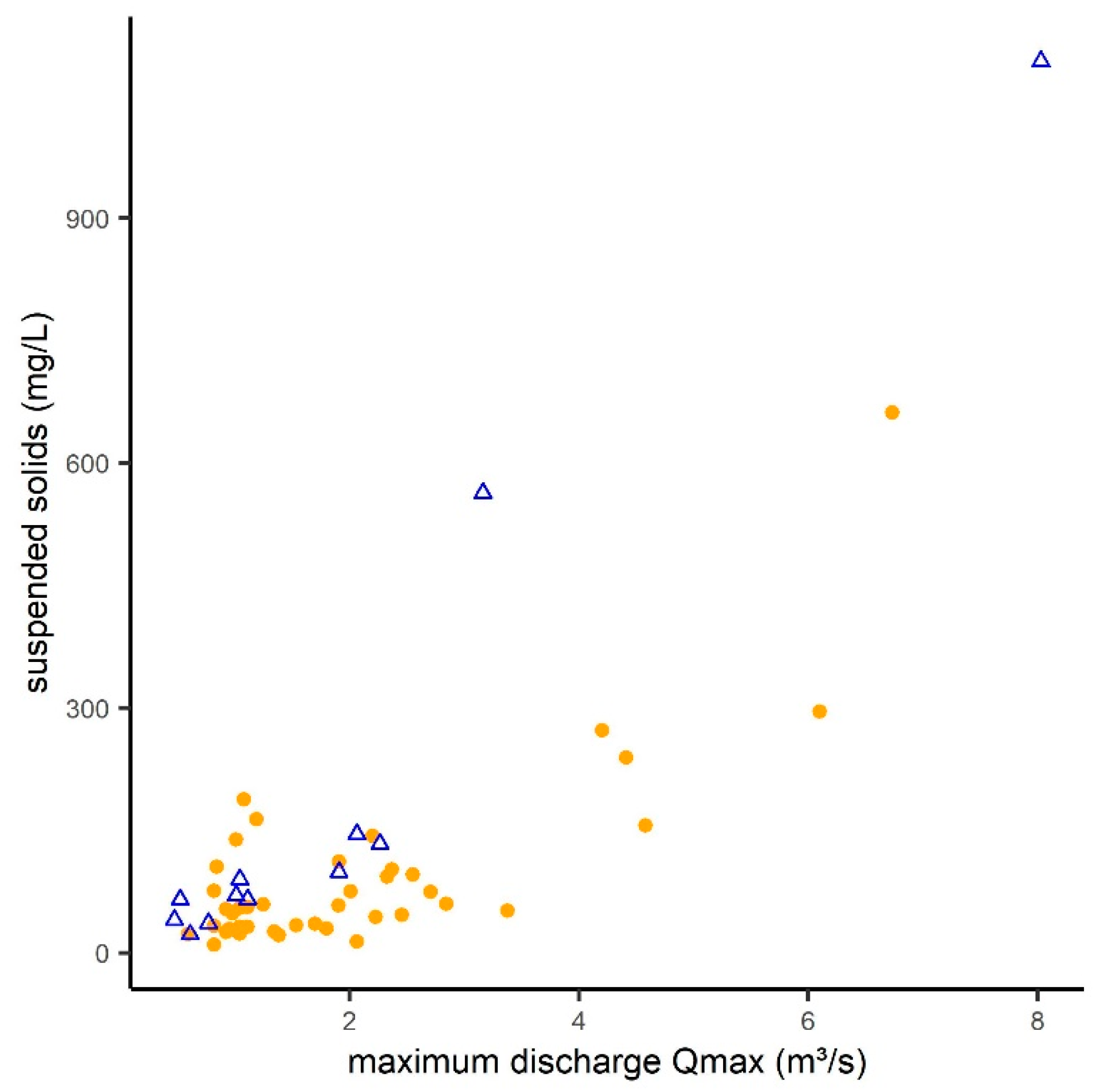
The highest event sampled with the LVS2 at a Q
max of 8.03 m
3 s
−1 has a mean suspended solids concentration of 1092 mg L
−1. This concentration is not diluted by included low or mean discharge conditions (as usual in LVS1 samples). Imagining a potential dilution of this sample, the concentration would be lower and thus lower the course of the rating curve (compare
Figure 6). This consideration substantiates the chosen procedure of limiting the course of the rating curve derived from LVS1 samples at the highest measured concentration when applied for load calculation.
Not only the lack of samples with a high discharge limits the applicability of the rating curve, but also the fact that discharge and substance transport can be decoupled because of the stochastic behavior of heavy rainfall events and resulting erosion processes. After a locally very heavy rainfall event, Fuchs et al. [
20] measured extreme concentrations of suspended solids (above 25,000 mg L
−1) and phosphorus (>20 mg L
−1) during two hours in the Kraichbach river at a resulting discharge around 5MQ only. Such temporary and locally limited rainfall events cannot be represented by a rating curve.
Horowitz [
4] states that rating curves should be adapted for single years instead of periods to gain better results for annual calculated river loads. In the case under review, this was not feasible due to the small number of samples for one year resulting from the long sampling periods of the LVSs. However, within the sampled years stationarity is assumed, which means that no or only little changes in sources or relations occur [
4]. As the rating curve covers the discharge distribution within the sampled years, it represents a robust mean state of the river and can be used to calculate annual loads within this time span. Given that the sampled years (2017–2021) represent a wide discharge spectrum, the transmission to other years (2003–2016) was done, although calculated loads will be less reliable for reasons of stationarity.
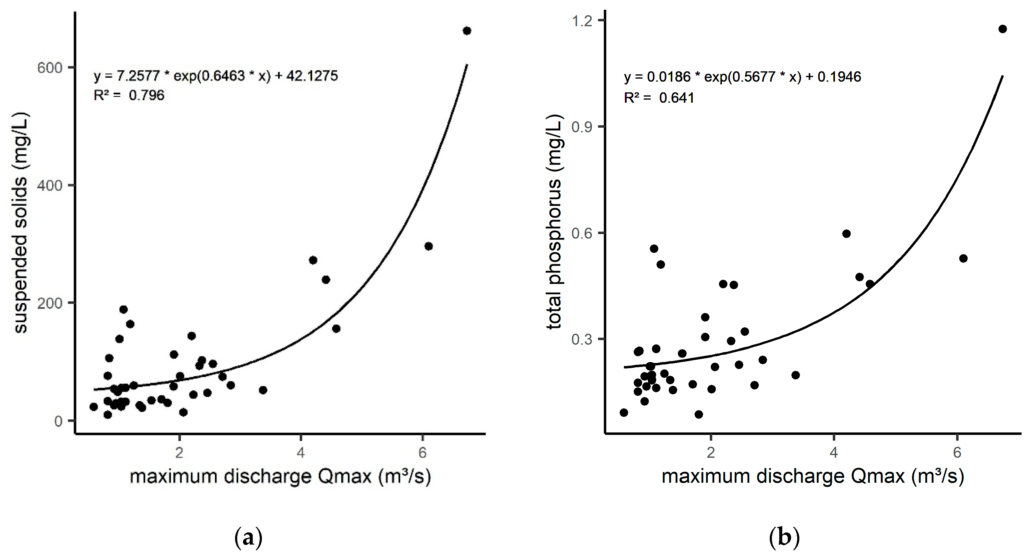
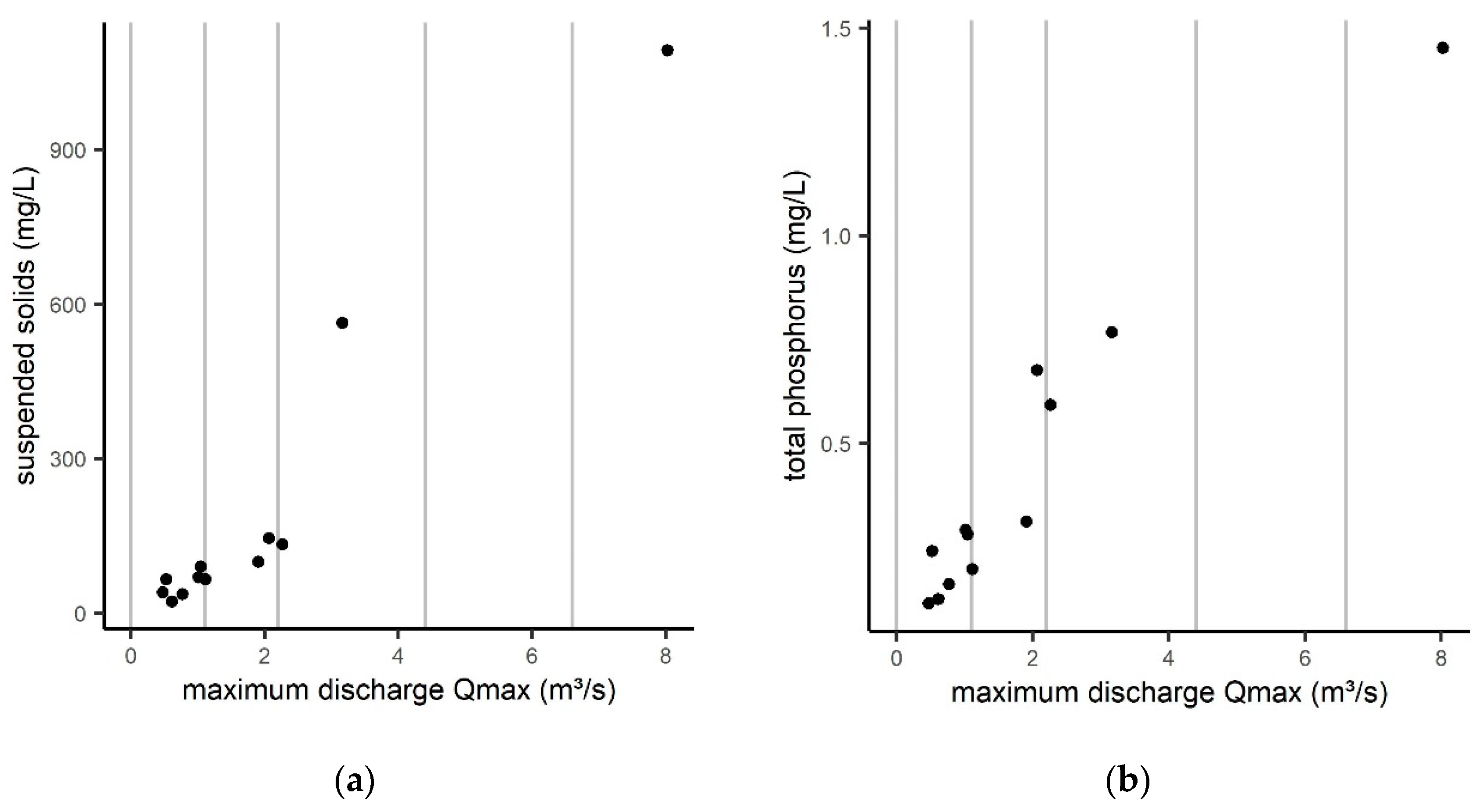
Low flow conditions (<MQ) as well have uncertainties, because in this discharge range, the concentrations vary a lot (compare
Figure 4). For example, for suspended solids, the concentrations reach up to 200 mg L
−1. Besides random local influences, internal processes and remobilization in the river occur during rain events after dry weather situations and could be responsible for higher concentrations in this discharge range.
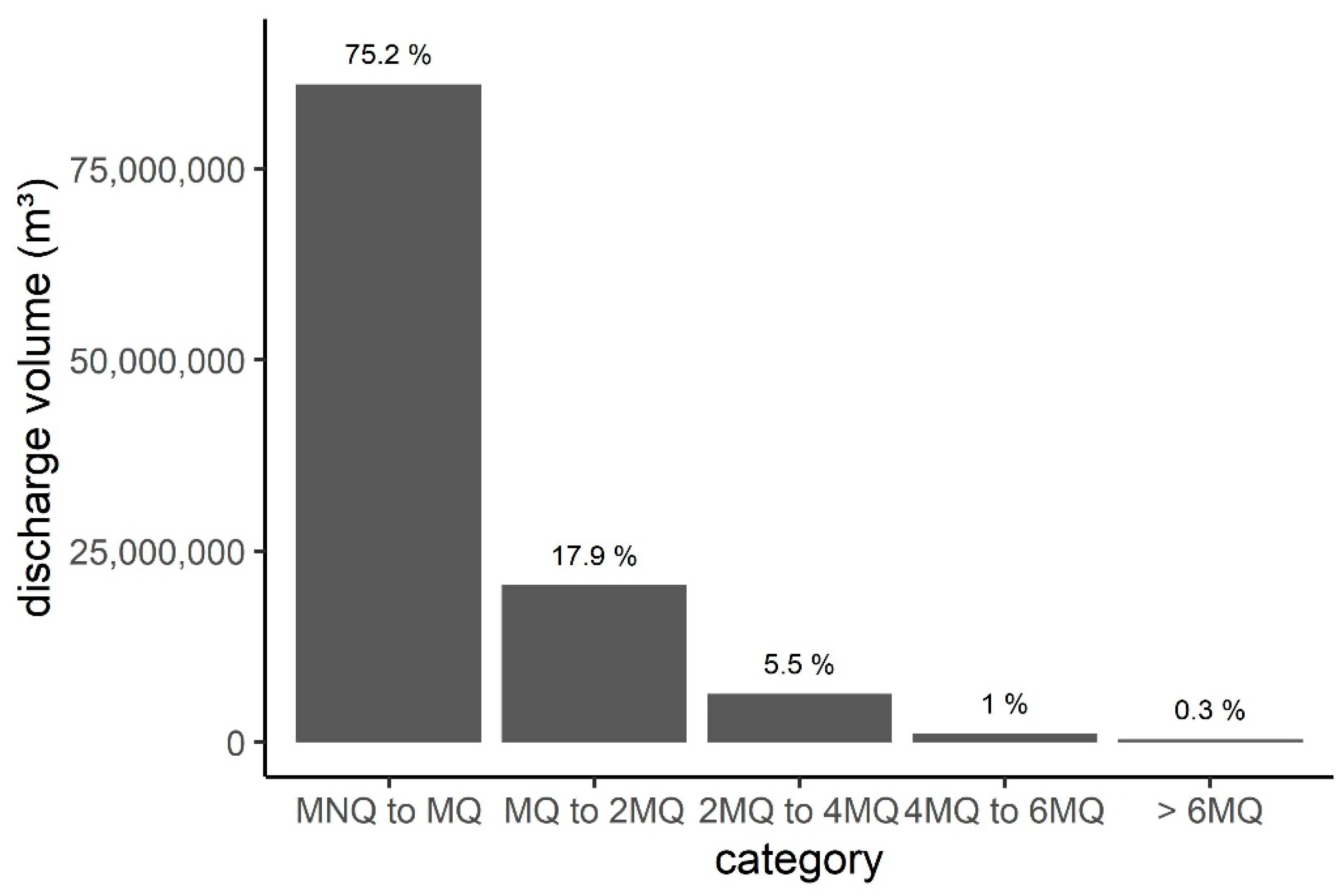
The distribution of the discharge volume during the period from 2003–2020 for the Kraichbach river of the gauging station ‘Ubstadt’ is shown in
Figure 7. The flow regime of the Kraichbach river is characterized by a high amount of low flow and mean flow (around 75%). Only one quarter of the discharge volume exceeds the mean discharge of 1.1 m
3 s
−1. A very small amount of around 5.5% of the annual discharge contributes to flow conditions between 2MQ and 4MQ. High flow conditions (>4MQ) only amount to 1.3% of the total discharge volume. The results clearly show that this small amount of volume influences the annual river load significantly. During heavy rainfall events, leading to high discharge in the river, the suspended solids and phosphorus concentration increase due to erosion input. During one sampling period with the LVS1 in 2018 with a Q
max of 6.7 m
3 s
−1 (covering eight days), around 770 t were transported (21% of the annual load). Fuchs et al. [
20] even reported that around 8% of the annual phosphorus load and 1700 t of the total suspended solids were transported in the Kraichbach river within only 16 h during a heavy rainfall event in 2003.
Considering the large discharge volume during low and mean flow conditions it becomes clear that valid concentrations are needed for this range. Even more important are valid concentrations in the high discharge range, since these contribute to a large extent to the annual load despite the low discharge volume in this range.
Despite the discussed uncertainties of the derived rating curve, composite samples are highly recommended for the calculation of annual river loads. They produce reliable results for all years where the maximum discharge is not exceeding the highest discharge that has occurred during the sampling periods with the LVS.
5. Conclusions
Large-volume samplers (LVSs) are a very useful method to sample surface waters. They are a great tool to be applied instead of grab samples to collect composite samples and better represent the actual river load. With different settings of the LVSs (quasi-continuous vs. event-based), different approaches are needed to calculate the annual river loads. Quasi-continuous sampling is the best method to use when annual river loads are the focus, because the sampling is easy to handle and the calculation of the river loads is clear. The second method applying event-based sampling should only be used when the concentrations themselves are of major interest. At the beginning, it looked like the second method would be the easier one with a ‘short’ sampling strategy, because only a few samples of each flow condition are needed to calculate the river loads. However, in reality, high labor input is needed and the monitoring is not easy to handle.
Moreover, the results of the LVSs can be used to balance pathway-specific emission inputs. The calculated loads represent the total substance input of the catchment, but with the knowledge of other emissions (e.g., wastewater treatment, combined sewer overflow), pathway-specific separation of the input sources can be made. The results can be used to validate modeled data. For the Kraichbach river, this is done by Allion et al. [
12] to verify the modeled sediment input in the catchment.
LVSs can be used very flexibly, depending on the monitored substances and the detailed research question.
One method of using the LVSs that was not applied in this study is to take homogenized samples [
15]. As the whole content of the LVS is homogenized before taking a sample, no settling time is needed. This offers the chance to perform a continuous instead of a quasi-continuous sampling.
For particulate-transported substances, the settled sample with supernatant water as used in this study is preferable. It offers the possibility to collect a large amount of solids representing a large discharge volume, which can be a major advantage in comparison to autosamplers. For this reason, a monitoring campaign using LVSs could be a great chance for the detection of substances such as microplastics that require a large sampling volume for robust results.


