Abstract
Accurate and reliable predictors selection and model construction are the key to medium and long-term runoff forecast. In this study, 130 climate indexes are utilized as the primary forecast factors. Partial Mutual Information (PMI), Recursive Feature Elimination (RFE) and Classification and Regression Tree (CART) are respectively employed as the typical algorithms of Filter, Wrapper and Embedded based on Feature Selection (FS) to obtain three final forecast schemes. Random Forest (RF) and Extreme Gradient Boosting (XGB) are respectively constructed as the representative models of Bagging and Boosting based on Ensemble Learning (EL) to realize the forecast of the three types of forecast lead time which contains monthly, seasonal and annual runoff sequences of the Three Gorges Reservoir in the Yangtze River Basin. This study aims to summarize and compare the applicability and accuracy of different FS methods and EL models in medium and long-term runoff forecast. The results show the following: (1) RFE method shows the best forecast performance in all different models and different forecast lead time. (2) RF and XGB models are suitable for medium and long-term runoff forecast but XGB presents the better forecast skills both in calibration and validation. (3) With the increase of the runoff magnitudes, the accuracy and reliability of forecast are improved. However, it is still difficult to establish accurate and reliable forecasts only large-scale climate indexes used. We conclude that the theoretical framework based on Machine Learning could be useful to water managers who focus on medium and long-term runoff forecast.
Highlights:
- (1)
- This study aims to summarize and compare the applicability and accuracy of different Feature Selection methods and Ensemble Learning models in medium and long-term runoff forecast.
- (2)
- Three typical methods (Filter, Wrapper, and Embedded) based on Feature Selection are employed to obtain predictors.
- (3)
- Two representative models (Bagging and Boosting) based on Ensemble Learning to realize the forecast.
1. Introduction
Refined medium and long-term runoff forecast technology is an important basis for the design, construction, and operation management of water conservancy and hydropower projects [1,2,3]. It is a basic key technology to realize the scientific allocation of water resources and improve the utilization efficiency of water resources and has important supporting significance for the dispatching management and optimal allocation of water resources [4,5,6]. With the rapid development of the social economy and the continuous improvement of science and technology, the ability of water resources regulation and control has been obviously improved. The practice of water resources regulation, such as unified regulation of basin water quantity, inter-basin water transfer, and joint regulation of super-large cascade reservoirs, has continued to advance, putting forward higher requirements for the forecast accuracy and forecast scale of medium and long-term runoff forecast. As such, its importance has become increasingly prominent [7,8,9,10]. In the unified regulation and management of water quantity in China’s Yangtze River, Yellow River, Pearl River and Huai River basins, medium and long-term runoff forecast are important scientific and theoretical bases for water resource allocation and regulation schemes, and the reliability, stability, and extensibility of the forecast results play a significant value [11,12].
However, monthly-seasonal-annual runoff forecast has always been a difficult point in hydrological science, both in theory and application. Compared with the short-term runoff forecast, the development is relatively slow and lags behind the actual production requirements [13,14]. It is of great theoretical and practical significance to establish a stable and reliable medium and long-term runoff forecast system by using fast-developing mathematics and computer technology while strengthening the collection and arrangement of basic data for runoff forecast [15,16].
In recent years, the fourth industrial revolution with Artificial Intelligence (AI) as its core has played an important role in hydrological forecasting, water resources regulation, and other fields. Among them, Machine Learning (ML) is an important branch of AI, and it is also a new discipline to study how to make computers learn rules from massive historical data through algorithms, so as to classify or predict new samples [17]. The development of forecasting model in ML has experienced several significant milestone time nodes. In 1952, Arthur Samuel firstly gave the definition and operable program of ML [18]. In 1958, Rosenblatt put forward the Perceptron Model which is the embryonic form of Artificial Neural Network (ANN) [19]. However, it was not until Werbos applied BP algorithm to build multilayer perceptron in 1982 that ANN developed rapidly [20]. In 1986, Quinlan proposed the earliest Decision Tree (DT), ID3 model [21]. Since then, C4.5 [22], CART [23] and other DT algorithm have flourished. In 1995, ML ushered in a major breakthrough. The Support Vector Machine (SVM) [24] presented by Vapnik and Cortes. It not only has a solid theoretical basis, but also has excellent experimental results. In 1999, Freund and Schapire put forward Adaptive Boosting (AdaBoost) [25], and in 2001 Breiman proposed Random Forest (RF) [26]. Both were based on DT theory and developed into representative algorithms of Boosting and Bagging [27,28], two important components of Ensemble Learning (EL).
When applying ML to medium and long-term runoff forecast, the first step is also the most important one, Feature Selection (FS), which is to extract accurate and appropriate features from the original data to the maximum extent by using relevant knowledge in the field of data analysis for the forecast model to achieve the best performance [29,30]. Due to the huge and messy data set, FS is a key step in building forecast models and also a highly iterative data preprocessing process [31]. This includes two reasons. First, FS can avoid Dimension Disaster due to too many attributes, which has similar motivation to dimension reduction (such as PCA, SVD, LDA, etc.), that is, trying to reduce the number of features in the original data set. However, these two methods are different. Dimension reduction mainly obtains new features by recombining the original features, while FS is to select subsets from the original features without changing the original feature space. Second, FS reduces data noise and the training difficulty of learners while removing the irrelevant feature. For medium and long-term runoff forecast, the FS is to find out the feature matching relationships between monthly-seasonal-annual runoff sequences and the previous climate indexes and select a certain number of features with physical causes, strong mutual independence and accurate and stable forecast performances as forecast factors. Climate Indexes include but are not limited to Sea Surface Temperature, El Nino index, Subtropical High, Circulation Index, Polar Vortex, Trade Wind, Warm Pool, Ocean Dipole, Solar Flux, etc.
Compared with the physical-driven runoff forecast model, the data-driven runoff forecast model based on machine learning not only reduces the difficulty of understanding runoff mechanism and the complexity of modeling, but also provides a new idea for runoff forecasting due to its solid theoretical basis and good performance. Many hydrologists use ML and Big Data Mining methods, such as ANN [32], SVM [3], Extreme Learning Machine (ELM) [33], Gradient Boosting Decision Tree (GBDT) [34], Relevance Vector Machine (RVM) [35], etc., to study and improve runoff forecast methods and models, to improve their ability to understand, predict and apply the evolution law of runoff phenomena.
In this paper, we summarize the Filter, Wrapper, and Embedded theories from FS based on ML and apply Partial Mutual Information (PMI), Recursive Feature Elimination (RFE), Classification and Regression Tree (CART) as the typical algorithms of the above three theories to select forecast factors suitable for medium and long-term runoff forecast. In the meanwhile, we also summarize the Bagging and Boosting frameworks from EL based-on ML and apply RF and XGB are the representative models of the above two frameworks to realize the forecast which lead time for the next month, next quarter, and next year, respectively. Besides, precision evaluation indexes are employed to compare and analyze forecast results of different schemes and models, which contain Relative Error (RE), Mean Value of Absolute Relative Error (MAPE), NASH Efficiency Coefficient (NSE), and Relative Root Mean Square Error (RRMSE). This paper is structured as follows. The theories of FS and EL are described in Section 2. A case study that contains catchment and research results is detailed in Section 3. The study is summarized and concluded in Section 4.
2. Methodology
2.1. Feature Selection
As a significant data preprocessing process, FS methods can be further subdivided into Filter, Wrapper, and Embedded [36]. In this paper, Partial Mutual Information (PMI), Recursive Feature Elimination (RFE) and Classification and Regression Tree (CART) are employed as the representative algorithms of Filter, Wrapper and Embedded, respectively. Accordingly, these three methods will build three schemes named Scheme A, B, and C. Each scheme includes three timescales predictors which are applied to monthly, seasonal, annual runoff forecast. Besides, assuming that the advance of the effectiveness of the climate indexes is one year, and ten predictors will be selected in each timescale forecast model. Due to the great difference of monthly runoff series in the year, the forecast factors of each month are different. Similarly, the same method is adopted for seasonal and annual forecast. Three types of FS are described as follow. In fact, most ML models themselves select features using weights. Here by using FS in advance models work faster or efficiently in addition to removing noise, and other issues.
2.2. Filter
Filter is based on the idea of greedy algorithm. By setting up a certain index to score, it then quantifies the relationship between each group of features and runoff, and removes the low-score features to obtain high-score features [37]. The FS process is independent of the subsequent learners, which is equivalent to “filtering” the original features and then training the model with the filtered features. According to the different indexes, Filter can be divided into four types: Distance, Correlation, Consistency, and Information Measurement [38]. The classical European, Mahalanobis, and Chebyshev Distance are all distance measurements. The commonly used Pearson, Spearman, and Kendall correlation coefficients all belong to the Correlation Measurement. Consistency measurement is not widely used because it only applies to discrete features. Information Measurement includes Mutual Information, Correlation Degree, Information Gain, and other methods [39].
Partial Mutual Information (PMI) which is based on Mutual information and presented by Sharma is employed as a typical method of Filter [40]. PMI estimates the correlation between the newly added forecast factors and the output variables, excluding the influence of the selected variables, i.e., PMI calculates the increment of correlation between input and output set when a new variable is added. It can be defined as [40,41]:
where E is a mathematical expectation, x is input and y is output of the selection model, and z is the selected set of forecast factors.
2.3. Wrapper
Unlike Filter which does not consider the subsequent learners, Wrapper directly takes the forecast performance of the learners to be used as the evaluation criterion for the FS [39,42]. In other words, FS is “wrapped” with the learners, and different learners will lead to different forecast factors. Las Vegas Wrapper (LVW) and Recursive Feature Elimination (RFE) are two common wrapped algorithms. LVW randomly generates feature subsets and uses cross-validation to estimate the errors of the learner. When the errors on the new feature subset are smaller, or the errors are equal but contain fewer features, the new feature subset is retained and recursively calculated until the target is reached [43]. RFE uses a base learner for multiple rounds of training. After each round of training, features of several weight coefficients are removed and the next round of training is conducted based on the new feature set, recursively calculating until the number of remaining features reaches the required [44]. By comparing the above methods, RFE is employed as the representative algorithm of wrapper in this paper. In the same way as Scheme A, ten forecast factors are selected as Scheme B according to RFE. Similarly, Scheme B includes three timescale predictors.
2.4. Embedded
In Filter and Wrapper, the feature selection process is obviously independent of learners training. In contrast, Embedded combines those two parts together in the same optimization process, in other words, feature selection is automatically done in the learner training process [39,45]. In order to achieve the result of synchronous optimization, Embedded relies on the specific forecast model and is mainly based on Regularization and DT method. The regularization method minimizes forecast error while preventing model over-fitting by referring to L1-norm (Lasso) or L2-norm (Ridge) as penalty terms of optimization function. In addition, DT include RF, GBDT etc. In this paper, Classification and Regression Tree (CART) is used to as the typical algorithm of Embedded, in the meanwhile, Scheme C is also coupled with sub-forecast models and provides three timescales. Due to the combination of the embedded strategy and forecast models, the specific theories are described in Section 2.2.
2.5. Ensemble Learning
The core theory of Ensemble Learning is to generate a large number of individual learners (sub-forecast models) and then synthesize the sub-forecast results through some strategies. If the individual learners adopt the same learning algorithm, it is called homogeneous integration, and the individual learners are called base learners. Otherwise, they are called heterogeneous integration and component learners, respectively [46]. Ensemble Learning can often achieve better forecast and forecast performance than a single one by combining multiple individual learners. Especially when the individual learner is a weak learner, the effect is more obvious. Therefore, most of the Ensemble Learning theories are based on weak learners. Different Ensemble learning algorithms are reflected in different combination strategies. Overall, Ensemble Learning can be divided into two categories: Bagging and Boosting. Boosting is suitable for scenarios where there is a strong dependency between individual learners, and they must be computed in serial. Bagging is suitable for scenarios where there is no strong dependency between individual learners and can be calculated in parallel [47,48,49].
In this paper, the Classification and Regression Tree (CART) is employed as a weak learner; Random Forest (RF) and Extreme Gradient Boosting (XGB) are used as a representative algorithm of Bagging and Boosting, respectively.
2.6. Classification and Regression Tree
In Machine Learning, Decision Tree (DT) is often used as a basic forecast model. The key to Decision Tree is to select the optimal partition attribute. Generally speaking, as the division process continues, we hope that the samples contained in the branch nodes of the decision tree belong to the same category as much as possible. In other words, the purity of the nodes should be getting higher and higher [50].
CART can be both a classification tree and a regression tree. When CART is a classification tree, Gini index is used as the basis for the node splitting. When CART is a regression tree, the Minimum Variance of samples is used as the basis for the node splitting [51]. When the regression trees are generated, the space will be recursively divided according to the optimal feature and value under the optimal feature until the stop condition is satisfied. The stop condition can be artificially set, such as setting the sample size of a certain node to be less than a given threshold C, or when the loss reduction value after segmentation is less than a given threshold ε [52].
For the generated CART, the category of each leaf node is the average of the labels falling on that leaf node. Assuming that the feature space is divided into M parts, i.e., there are now M leaf nodes , and the corresponding data quantity is , the predicted values of leaf nodes are:
CART is also a binary tree, which is divided according to the value of the feature every time. If the value S of the feature J is segmented, the two regions after segmented are respectively:
Calculate the estimated values C1 and C2 of R1 and R2 respectively, and then calculate the loss after splitting according to (j,s):
Equations (4) and (5) will are recursively continued until the end condition is met.
2.7. Random Forest
Random Forest (RF) is present by Breiman and as the most widely used Bagging algorithm. As the flow chart shown in Figure 1, the process contains three parts. Firstly, using Bootstrap sampling method, N sub-training sets will be extracted from the original training set. Secondly, using CART as a sub-forecast model, runoff is simulated, and N sub-results are obtained. Finally, the weighted average of the N sub-results is carried out to obtain the final forecast result [53,54].
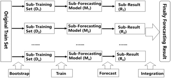
Figure 1.
Flow chart of Bagging algorithm.
2.8. Extreme Gradient Boosting
Extreme Gradient Boosting (XGB) is presented by Tianqi Chen and as an enhancement of GBDT algorithm [55]. Both XGB and GBDT are based on Boosting algorithm whose flow chart is shown as Figure 2. The main idea of XGB is to step up the training process, using all samples for each round of training and changing the weights of samples. The loss function is used to fit the residual error. The goal of each training round is to fit the residual error of the previous round, and the forecast result is the weighted average of the forecast results of each round when the residual error is small enough or reaches the number of iterations [56,57].
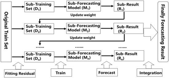
Figure 2.
Flow chart of Boosting algorithm.
XGB is essentially an addition model, and its sub-decision tree model only uses CART regression tree. Assuming the training sample is , and x could be a multi-dimensional vector. represents the predicted value after the t-th iteration, represents the increment of the t-th iteration:
Model learning is a NP-C process to find the optimal solution and always uses a heuristic strategy. Assuming that
is the observed values of training samples in the iterative process;
is the simulated values; L is the loss function and
is the regularization function, then the objective function OBJ of XGB can be defined as:
In the regularization function, T is the number of leaf nodes;
is the fraction of leaf nodes;
is the regularization parameter and
is the minimum loss required to further divide the leaf nodes. Penalizing the number of leaf nodes is equivalent to pruning in training, so that the model is not prone to over-fitting.
3. Case Study
3.1. Study Area
In the paper, we apply the proposed methodology to the Three Gorges Reservoir which is located in the Yangtze River Basin. The Yangtze River is the longest and most abundant river in China, with a total length of 6300 km. As the third longest river in the world, its total amount of water resources is 961.6 billion cubic meters, accounting for about 36% of the total river runoff in the country, 20 times that of the Yellow River. Above Yichang is the upper reaches of the Yangtze River, with a length of 4504 km and a basin area of one million square meters. Yichang to Hukou is the middle reaches, with a length of 955 km and a basin area of 0.68 million square meters. Below Hukou is the downstream, with a length of 938 km and a basin area of 0.12 million square meters. The Three Gorges Reservoir, located in Yichang City, is the largest water conservancy project in China and has a series of functions such as flood control, irrigation, shipping, and power generation. Its control basin accounts for about 60% of the Yangtze River basin, with a total area of 1084 square meters, a total capacity of 30.3 billion cubic meters and an average flow of 15,000 cubic meters per second for many years [58,59].
3.2. Predictors
The forecast factors are based on 130 remote-related climate indexes provided by the National Climate Center (China) (https://cmdp.ncc-cma.net/Monitoring/cn_index_130.php accessed on 4 April 2021). Climate indexes contain three parts. The first part includes 88 atmospheric circulation indexes such as Subtropical High, Polar Vortex, Subtropical High Ridge, Zonal/Meridional Circulation, Pattern Index, Wind Index, etc. All the atmospheric circulation indexes have an exact location, strength and range. The second part is about 26 sea surface temperature indexes which include NINO 1 + 2 SSTA Index, NINO 3.4 SSTA Index, Indian Ocean Basin-Wide Index, South Indian Ocean Dipole Index, etc. The third part includes 16 other indexes such as Cold Air Activity Index, Total Sunspot Number Index, Southern Oscillation Index, etc. The detail of 130 remote-related climate indexes can be found on the website of National Climate Center (China).
As mentioned in Section 2.1, schemes named A, B, C as three kinds forecast factors, which are used as the representatives of theory of Filter, Wrapper and Embedded. Due to the space limitation in this paper, only the predictors of January in monthly forecast at Three Gorges Reservoir are shown as an example. The predictors are as follows in the Table 1. Since the factors are all previous year, the first number means the specific month. For example, 5_Western Pacific Subtropical High Intensity Index represents the value of this climate index in May last year.

Table 1.
Forecast factors of January runoff at Three Gorges Reservoir.
3.3. Precision Evaluation Indexes
The model accuracy analysis is based on six performance indexes that have been widely used to evaluate the good-ness-of-fit of hydrologic models. Although there are other hydrological evaluation indexes, we intend to use Square of Correlation Coefficient (R2), Relative Root Mean Square Error (RRMSE), Relative Error (RE), Mean Absolute Percentage Error (MAPE), Nash-Sutcliffe Coefficient of Efficiency (NSE) and Qualification Rate (QR). In the following description, , , and are observed values, simulated values, mean of observed sequences and mean of simulated sequences, respectively. The values of n and N are the qualified length and total length of data set, respectively.
- (1)
- Square of correlation coefficient (R2)R2 is one of the most employed criteria to evaluate model efficiency. Its range between −1 and 1 (perfect fit) and it is defined as:
- (2)
- Relative Root Mean Square Error (RRMSE)RRMSE is based on RMSE which is not suitable for comparing different magnitudes of streamflow, i.e., RRMSE which ranges from −1 and 1 shows a good performance to compare runoff sequences in different river basins. RRMSE is calculated as [60]:
- (3)
- Relative Error (RE) and Mean Absolute Percentage Error (MAPE)RE and MAPE are conventional criteria to show the results in each data point. There are given by:
- (4)
- Nash-Sutcliffe Coefficient of Efficiency (NSE)
The NSE is one of the best performance metrics for reflecting the overall fit of a hydrograph. It varies from −∞ and 1 (perfect fit). If the NSE value between 0 and 1, it means an acceptable model performance. If NSE value is lower than 0, it indicates that mean value of the series is a better estimation than the constructed model. NSE is defined as [61]:
3.4. Monthly Forecast
Python is adopted as the programming platform this time, including open-source databases Numpy, Pandas, Scikit-Learn, etc. The runoff sequences are calibrated over the 37-year period 1965–2001 and validated over the 15-year period 2002–2016. The parameters of RF and XGB models in different scales are determined by the fitting effect in calibration. In order to verify the adaptability and accuracy of the three predictors selection methods and the two types of machine learning for medium and long-term forecast models in different timescales, the forecast lead time focus on one month, one quarter and one year, respectively.
As shown in Figure 3, for the situation of different models with same predictors’ schemes, the accuracy in calibration of XGB is better than that of RF. Scatters in XGB are much closer the 1:1 line which means a perfect fitness. In the meanwhile, all the values on the scatterplots are evenly located at both sides of orange line, show little indication of system deviation. For another situation of same models with different predictors’ schemes, it shows a similar accuracy and adaptation. It is difficult to compare the performance of the Scheme A, Scheme B, and Scheme C from the graphs. The precision evaluation indexes are shown in the following Table 2 which contains the specific values towards three schemes and two monthly forecast models. Data in the table further verify the above conclusions.
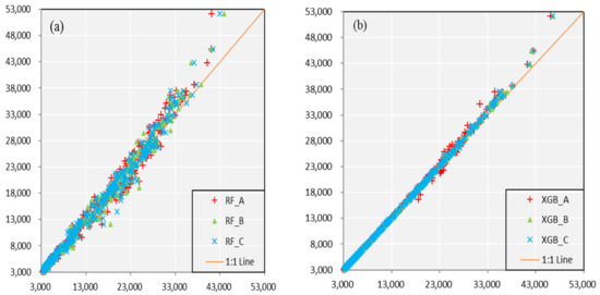
Figure 3.
Scatterplots of monthly observed and simulated runoff sequences estimated from (a) RF and (b) XGB model in calibration. The orange line represents 1:1 line which means a perfect fitness. The vertical axis is the observed runoff value and the horizontal axis is the simulated runoff value.
Table 2.
Precision evaluation indexes of RF and XGB monthly forecast model in the period of calibration.
In the validation period, the specific RE is shown as Figure 4 and Table 3. For the heatmaps, red indicates that the predicted is greater than the observed value, and blue indicates that the predicted is less than the measured value. According to the value of RE, set the legend to +50% at the maximum and −50% at the minimum and the darker the color, the greater the absolute value of the RE. In the horizontal direction of Figure 4, the left and right is RF and XGB model. In the vertical direction, there are Scheme A, B, and C, respectively.
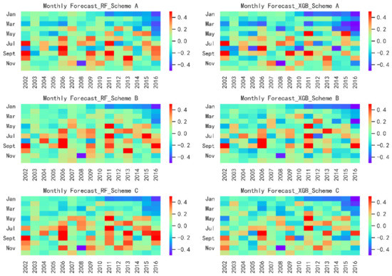
Figure 4.
Heatmaps plots of monthly observed and simulated runoff sequences estimated from RF and XGB model in validation. The legend is set to +50% at the maximum and −50% at the minimum of all the heatmaps and the lighter the color, the smaller the absolute value of the RE.
Table 3.
Precision evaluation indexes of RF and XGB monthly forecast model in the period of validation.
Generally speaking, the forecasts of Jan and July to Oct are much worse than other months. Figure 5 presents an enhanced boxplot named letter-value plot [62]. Standard boxplots consist of the outliers, maximum, upper quartile, median, lower quartile, minimum and outliers from top to bottom. Boxplots are useful to illustrate the rough information about the distribution of the variables but do not take advantage of precise estimates of tail behavior, i.e., the specific data distribution cannot be displayed. As for letter-value plot, in addition to drawing the original quartiles, it continues to draw 8th, 16th, 32nd, etc., and the width and color depth of each box correspond to the corresponding sample size. Based on letter-value plots, we could tell the concentration and dispersion of monthly runoff, which not only shows the position of the data quintiles, but also shows the probability density of any position. As the runoff of Jan, July to Oct shown in Figure 5, the distributions of observed values are extremely scattered, and the annual differences are large. Transversely, the distributions are relatively uniform, and the repeat abilities are low. This feature of runoff increases the difficulty of forecast.
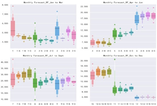
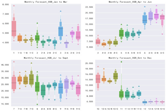
Figure 5.
Letter-value plots of monthly observed and simulated runoff sequences estimated from RF and XGB model of Scheme A, B, C in validation. 1-A means the result of using Scheme A as predictors in Jan and others have an analogous meaning. The vertical axis is the observed runoff value, and the horizontal axis is the simulated runoff value.
In general, the horizontal comparison shows that XGB model has a slightly better forecast result than RF model under the same forecast factors. At the same time, the vertical comparison shows that for the same forecast model, Scheme B has the highest accuracy, and Schemes A and C are similar.
3.5. Seasonal Forecast
When forecasting the runoff in the next quarter, 130 remote-related climate indexes with an advance of one year are still used as forecast factors, and the total runoff values of each quarters are used as forecast targets, with the calibration and validation period the same as monthly forecast. Figure 6 and Table 4 show the forecast results of the two models in calibration, and similar conclusions which according to Figure 3 and Table 2 can be obtained.
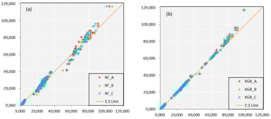
Figure 6.
Scatterplots of seasonal observed and simulated runoff sequences estimated from (a) RF and (b) XGB model in calibration. The orange line represents 1:1 line which means a perfect fitness. The vertical axis is the observed runoff value, and the horizontal axis is the simulated runoff value.
Table 4.
Precision evaluation indexes of RF and XGB seasonal forecast model in the period of calibration.
As can be seen from Figure 7, in general, the forecast results of the validation period are similar for the two models with the same forecast factor scheme. Except for the poor forecast results in 2006, 2009 and the first quarter combined Scheme A, the second quarter’s combined Scheme B and the third quarter combined Scheme C from 2010 to 2016, the results are still acceptable. Table 5 shows similar results to those shown in Table 3, except for further demonstration of the above results, the results of Scheme B are the best, slightly better than those of Scheme A and C, and the latter two results are parallel.
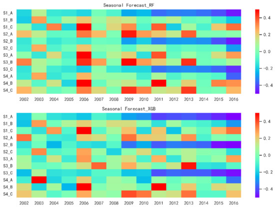
Figure 7.
Heatmaps plots of seasonal observed and simulated runoff sequences estimated from RF and XGB model in validation. The legend is set to +50% at the maximum and −50% at the minimum of all the heatmaps and the lighter the color, the smaller the absolute value of the RE. S1_A means the result of using Scheme A as predictors in first season and others have an analogous meaning.
Table 5.
Precision evaluation indexes of RF and XGB seasonal forecast model in the period of validation.
3.6. Annual Forecast
When forecasting the runoff for the next year, 130 remote-related climate indexes with an advance of one year are still used as forecast factors, and the total runoff values of each years are used as forecast targets, with the calibration and validation period the same as monthly forecast. Because the data sequence is short, only the MAPE is used to evaluate the forecast results. Similar to the previous description, scatterplots are employed to illustrate the accuracy shown in Figure 8 and Table 6. There still displays a closely phenomenon that XGB is better than RF model in calibration. It is worth noting that, for the annual forecast, the RF shows that the lower observation contributes under-estimates, and the higher observation contributes the over-estimates. As for XGB, most cases are overestimated, and with the increase of observed values, the overestimation phenomenon becomes more obvious. One possible reason is that the annual runoff varies greatly from year to year. In the period of model building, some extreme values significantly affect the modelling process, resulting in overestimation/underestimation on the whole. We will pay attention to this in the follow-up research.

Figure 8.
Scatterplots of annual observed and simulated runoff sequences estimated from (a) RF and (b) XGB model in calibration. The orange line represents 1:1 line which means a perfect fitness. The vertical axis is the observed runoff value and the horizontal axis is the simulated runoff value.
Table 6.
Precision evaluation indexes of RF and XGB seasonal forecast model in the period of calibration and validation.
Figure 9 and Table 6 demonstrates a specific RE for three schemes in each year. For the case of RF/XGB models under different forecast factors, Scheme B represents the best forecast skill. For the situation of three schemes under different models, XGB shows a higher accuracy and stability than RF model both in validation and calibration.
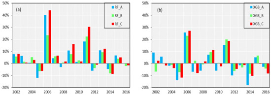
Figure 9.
Bar plots of RE of annual observed and simulated runoff sequences estimated from (a) RF and (b) XGB model in validation. Blue, green and red respectively represent the result of Scheme A, B and C.
4. Conclusions
For the medium and long-term runoff forecast on the monthly-seasonal-annual scale, the difficulty and emphasis include two parts. The first is to select accurate and stable forecast factors with certain physical causes, and the second is to build forecast models with clear theory and good forecast.
In this paper, we summarize three typical methods of Feature Selection theory based on Machine Learning in the selection of forecast factors and employ PMI, RFE, and CART as typical algorithms of Filter, Wrapper, and Embedded, respectively, to obtain three sets of forecast factor schemes. In the meanwhile, we summarize two typical theories of Ensemble Learning based on Machine Learning, and selected RF and XGB as typical models for Bagging and Boosting to simulate and forecast runoff sequences. The above forecasting frameworks are applied to the Three Gorges Reservoir in the Yangtze River Basin to realize monthly-seasonal-annual runoff forecast. Through the forecast results in the periods of calibration and validation, the following conclusions can be obtained:
- (1)
- For three schemes, Scheme B shows the best forecast skills, highest accuracy and stability when comparing the same forecast lead time and models. Scheme A and Scheme C have similar results and are slightly inferior to Scheme B. It illustrates that taking the forecast performance of the learners to be used as the evaluation criterion for the FS is an effective and efficient approach.
- (2)
- For two models, XGB shows a better forecast result than RF model during the calibration period when comparing the same forecast lead time and predictors. Furthermore, in the validation period, XGB also shows a smaller forecast error if only taking Scheme B as a comparison. This is not to say that XGB is a better model than RF for two reasons. Firstly, it requires more basin data to verify whether there are differences in forecasting skill. Secondly, among some forecast factor schemes, RF displays a better performance. Therefore, the Ensemble Learning algorithms based on two different frameworks are suitable for medium and long-term runoff forecast.
- (3)
- For three different forecast lead time, it shows an interesting phenomenon. According to the most commonly used MAPE index, the annual runoff forecasting error is the smallest. MAPE is 8.34% and 7.11% in RF and XGB model, respectively, while the monthly and seasonal runoff forecast results are similar, and MAPE floats around 16%. This demonstrates that with the increase of the runoff magnitudes, the instability and non-uniformity of the distribution of the extreme value series are reduced, and the accuracy and stability of forecast are improved.
Author Contributions
Conceptualization, Y.L. and H.H.; Data curation, Y.L. and D.W.; Formal analysis, Y.L. and J.W.; Funding acquisition, Y.X. and Y.L.; Investigation, Y.L. and B.L.; Methodology, Y.L. and B.X.; Project administration, Y.L.; Resources, Y.L.; Software, Y.L.; Supervision, Y.L.; Validation, Y.L.; Visualization, Y.L.; Writing—original draft, Y.L. and H.H.; Writing—review & editing, Y.L. and H.H. All authors have read and agreed to the published version of the manuscript.
Funding
This research was funded by Yueping XU, grant number LZ20E090001 (the Major Project of Zhejiang Natural Science Foundation). And also funded by Yujie LI, grant number RB2012 (the Science and Technology Project of Zhejiang Provincial Water Resources Department)”.
Institutional Review Board Statement
Not applicable.
Informed Consent Statement
Not applicable.
Data Availability Statement
MDPI is committed to supporting open scientific exchange and enabling our authors to achieve best practices in sharing and archiving research data. We encourage all authors of articles published in MDPI journals to share their research data. More details in section “MDPI Research Data Policies” at https://www.mdpi.com/ethics accessed on 4 April 2021.
Acknowledgments
The study is financially supported by the Major Project of Zhejiang Natural Science Foundation, China (LZ20E090001) and the Science and Technology Project of Zhejiang Provincial Water Resources Department (RB2012). We gratefully acknowledge the anonymous editors and reviewers for their insightful and professional comments, which greatly improved this manuscript.
Conflicts of Interest
The authors declare no conflict of interest.
References
- Bennett, J.C.; Wang, Q.J.; Li, M.; Robertson, D.E.; Schepen, A. Reliable long-range ensemble streamflow forecasts: Combining calibrated climate forecasts with a conceptual runoff model and a staged error model. Water Resour. Res. 2016, 52, 8238–8259. [Google Scholar] [CrossRef]
- Bennett, J.C.; Wang, Q.J.; Robertson, D.E.; Schepen, A.; Li, M.; Michael, K. Assessment of an ensemble seasonal streamflow forecasting system for Australia. Hydrol. Earth Syst. Sci. 2017, 21, 6007–6030. [Google Scholar] [CrossRef]
- Breiman, L. Random forests. Mach. Learn. 2001, 45, 5–32. [Google Scholar] [CrossRef]
- Breiman, L.; Friedman, J.; Olshen, R.; Stone, C. Classification and Decision Trees; Wadsworth Inc.: Belmont, CA, USA, 1984. [Google Scholar]
- Charles, S.P.; Wang, Q.J.; Ahmad, M.-U.-D.; Hashmi, D.; Schepen, A.; Podger, G.; Robertson, D.E. Seasonal streamflow forecasting in the upper Indus Basin of Pakistan: An assessment of methods. Hydrol. Earth Syst. Sci. 2018, 22, 3533–3549. [Google Scholar] [CrossRef]
- Chen, T.; Guestrin, C. Xgboost: A scalable tree boosting system. In Proceedings of the 22nd ACM SIGKDD International Conference on Knowledge Discovery and Data Mining, San Francisco, CA, USA, 13–17 August 2016. [Google Scholar]
- Ang, J.C.; Mirzal, A.; Haron, H.; Hamed, H.N.A. Supervised, Unsupervised, and Semi-Supervised Feature Selection: A Review on Gene Selection. IEEE/ACM Trans. Comput. Biol. Bioinform. 2015, 13, 971–989. [Google Scholar] [CrossRef] [PubMed]
- Choubin, B.; Zehtabian, G.; Azareh, A.; Rafiei-Sardooi, E.; Sajedi-Hosseini, F.; Kişi, Ö. Precipitation forecasting using classification and regression trees (CART) model: A comparative study of different approaches. Environ. Earth Sci. 2018, 77, 314. [Google Scholar] [CrossRef]
- Cortes, C.; Vapnik, V. Support-vector networks. Mach. Learn. 1995, 20, 273–297. [Google Scholar] [CrossRef]
- Dai, Z.; Mei, X.; Darby, S.E.; Lou, Y.; Li, W. Fluvial sediment transfer in the Changjiang (Yangtze) river-estuary depositional system. J. Hydrol. 2018, 566, 719–734. [Google Scholar] [CrossRef]
- Erdal, H.I.; Karakurt, O. Advancing monthly streamflow forecast accuracy of CART models using ensemble learning paradigms. J. Hydrol. 2013, 477, 119–128. [Google Scholar] [CrossRef]
- Fernando, T.; Maier, H.; Dandy, G. Selection of input variables for data driven models: An average shifted histogram partial mutual information estimator approach. J. Hydrol. 2009, 367, 165–176. [Google Scholar] [CrossRef]
- Frederick, L.; Vanderslice, J.; Taddie, M.; Malecki, K.; Gregg, J.; Faust, N.; Johnson, W.P. Contrasting regionalgboost and national mechanisms for predicting elevated arsenic in private wells across the United States using classification and re-gression trees. Water Res. 2016, 91, 295–304. [Google Scholar] [CrossRef]
- Freund, Y.; Schapire, R.; Abe, N. A short introduction to boosting. J. Jpn. Soc. Artif. Intell. 1999, 14, 1612. [Google Scholar]
- Hadi, S.J.; Tombul, M. Monthly streamflow forecasting using continuous wavelet and multi-gene genetic pro-gramming combination. J. Hydrol. 2018, 561. [Google Scholar] [CrossRef]
- Han, J.; Mao, K.; Xu, T.; Guo, J.; Zuo, Z.; Gao, C. A Soil Moisture Estimation Framework Based on the CART Algo-rithm and Its Application in China. J. Hydrol. 2018, 563, 65–75. [Google Scholar] [CrossRef]
- Hofmann, H.; Wickham, H.; Kafadar, K. Letter-Value Plots: Boxplots for Large Data. J. Comput. Graph. Stat. 2017, 26, 469–477. [Google Scholar] [CrossRef]
- Hong, M.; Wang, D.; Wang, Y.; Zeng, X.; Ge, S.; Yan, H.; Singh, V.P. Mid- and long-term runoff forecasts by an improved phase-space reconstruction model. Environ. Res. 2016, 148, 560–573. [Google Scholar] [CrossRef] [PubMed]
- Humphrey, G.B.; Gibbs, M.S.; Dandy, G.C.; Maier, H.R. A hybrid approach to monthly streamflow forecasting: Integrating hydrological model outputs into a Bayesian artificial neural network. J. Hydrol. 2016, 540, 623–640. [Google Scholar] [CrossRef]
- Koller, D.; Sahami, M. Toward optimal feature selection. In Proceedings of the Thirteenth International Conference on International Conference on Machine Learning, Bari, Italy, 3–6 July 1996. [Google Scholar]
- Liang, Z.; Li, Y.; Hu, Y.; Li, B.; Wang, J. A data-driven SVR model for long-term runoff forecast and uncertainty analysis based on the Bayesian framework. Theor. Appl. Climatol. 2017, 133, 137–149. [Google Scholar] [CrossRef]
- Liang, Z.; Tang, T.; Li, B.; Liu, T.; Wang, J.; Hu, Y. Long-term streamflow forecasting using SWAT through the in-tegration of the random forests precipitation generator: Case study of Danjiangkou Reservoir. Hydrol. Res. 2017, 49, 1513–1527. [Google Scholar] [CrossRef]
- Lin, G.-F.; Chen, L.-H. A non-linear rainfall-runoff model using radial basis function network. J. Hydrol. 2004, 289, 1–8. [Google Scholar] [CrossRef]
- Liu, H.; Setiono, R. A probabilistic approach to feature selection-a filter solution. In Proceedings of the Thirteenth International Conference on International Conference on Machine Learning, Bari, Italy, 3–6 July 1996. [Google Scholar]
- Liu, H.; Yu, L. Toward integrating feature selection algorithms for classification and clustering. IEEE Trans. Knowl. Data Eng. 2005, 17, 491–502. [Google Scholar] [CrossRef]
- Liu, Y.; Ye, L.; Qin, H.; Hong, X.; Ye, J.; Yin, X. Monthly streamflow forecasting based on hidden Markov model and Gaussian Mixture Regression. J. Hydrol. 2018, 561, 146–159. [Google Scholar] [CrossRef]
- Lu, X.; Ju, Y.; Wu, L.; Fan, J.; Zhang, F.; Li, Z. Daily pan evaporation modeling from local and cross-station data using three tree-based machine learning models. J. Hydrol. 2018, 566, 668–684. [Google Scholar] [CrossRef]
- Lyu, Y.; Zheng, S.; Tan, G.; Shu, C. Effects of Three Gorges Dam operation on spatial distribution and evolution of channel thalweg in the Yichang-Chenglingji Reach of the Middle Yangtze River, China. J. Hydrol. 2018, 565, 429–442. [Google Scholar] [CrossRef]
- Nash, J.E.; Sutcliffe, J.V. River flow forecasting through conceptual models part I—A discussion of principles. J. Hydrol. 1970, 10, 282–290. [Google Scholar] [CrossRef]
- Ng, A.Y. Feature Selection, L 1 vs. L 2 Regularization; Computer Science Department, Stanford University: Stanford, CA, USA, 2004. [Google Scholar]
- O’Neil, G.L.; Goodall, J.L.; Watson, L.T. Evaluating the potential for site-specific modification of LiDAR DEM derivatives to improve environmental planning-scale wetland identification using Random Forest classification. J. Hydrol. 2018, 559, 192–208. [Google Scholar] [CrossRef]
- Paradis, D.; Lefebvre, R.; Gloaguen, E.; Rivera, A. Predicting hydrofacies and hydraulic conductivity from direct-push data using a data-driven relevance vector machine approach: Motivations, algorithms, and application. Water Resour. Res. 2015, 51, 481–505. [Google Scholar] [CrossRef]
- Peters, J.; De Baets, B.; Samson, R.; Verhoest, N.E.C. Modelling groundwater-dependent vegetation patterns using ensemble learning. Hydrol. Earth Syst. Sci. 2008, 12, 603–613. [Google Scholar] [CrossRef]
- Pullanagari, R.R.; Kereszturi, G.; Yule, I. Integrating Airborne Hyperspectral, Topographic, and Soil Data for Estimating Pasture Quality Using Recursive Feature Elimination with Random Forest Regression. Remote. Sens. 2018, 10, 1117. [Google Scholar] [CrossRef]
- Quinlan, J.R. Induction of Decision Trees. Mach. Learn. 1986, 1, 81–106. [Google Scholar] [CrossRef]
- Quinlan, J.R. C4.5: Programs for Machine Learning; Morgan Kaufmann Publishers: Burlington, MA, USA, 1992. [Google Scholar]
- Rodriguez-Galiano, V.; Luque-Espinar, J.; Chica-Olmo, M.; Mendes, M. Feature selection approaches for predictive modelling of groundwater nitrate pollution: An evaluation of filters, embedded and wrapper methods. Sci. Total. Environ. 2018, 624, 661–672. [Google Scholar] [CrossRef]
- Rosenblatt, F. The perceptron: A probabilistic model for information storage and organization in the brain. Psychol. Rev. 1958, 65, 386–408. [Google Scholar] [CrossRef] [PubMed]
- Saeys, Y.; Inza, I.; Larrañaga, P. A review of feature selection techniques in bioinformatics. Bioinformatics 2007, 23, 2507–2517. [Google Scholar] [CrossRef]
- Samuel, A.L. Some Studies in Machine Learning Using the Game of Checkers. IBM J. Res. Dev. 1959, 3, 210–229. [Google Scholar] [CrossRef]
- Schepen, A.; Zhao, T.; Wang, Q.; Zhou, S.; Feikema, P. Optimising seasonal streamflow forecast lead time for oper-ational decision making in Australia. Hydrol. Earth Syst. Sci. 2016, 20, 4117–4128. [Google Scholar] [CrossRef]
- Schick, S.; Rössler, O.; Weingartner, R. Monthly streamflow forecasting at varying spatial scales in the Rhine basin. Hydrol. Earth Syst. Sci. 2018, 22, 929–942. [Google Scholar] [CrossRef]
- Sharma, A. Seasonal to interannual rainfall probabilistic forecasts for improved water supply management: Part 1—A strategy for system predictor identification. J. Hydrol. 2000, 239, 232–239. [Google Scholar] [CrossRef]
- Shen, K.-Q.; Ong, C.-J.; Li, X.-P.; Wilder-Smith, E.P.V. Feature selection via sensitivity analysis of SVM probabilistic outputs. Mach. Learn. 2007, 70, 1–20. [Google Scholar] [CrossRef]
- Shortridge, J.E.; Guikema, S.D.; Zaitchik, B.F. Machine learning methods for empirical streamflow forecast: A comparison of model accuracy, interpretability, and uncertainty in seasonal watersheds. Hydrol. Earth Syst. Sci. 2016, 20, 2611–2628. [Google Scholar] [CrossRef]
- Singh, K.P.; Gupta, S.; Mohan, D. Evaluating influences of seasonal variations and anthropogenic activities on alluvial groundwater hydrochemistry using ensemble learning approaches. J. Hydrol. 2014, 511, 254–266. [Google Scholar] [CrossRef]
- Šípek, V.; Daňhelka, J. Modification of input datasets for the Ensemble Streamflow Forecast based on large-scale climatic indices and weather generator. J. Hydrol. 2015, 528, 720–733. [Google Scholar] [CrossRef]
- Sun, W.; Trevor, B. A stacking ensemble learning framework for annual river ice breakup dates. J. Hydrol. 2018, 561, 636–650. [Google Scholar] [CrossRef]
- Tang, G.; Long, D.; Behrangi, A.; Wang, C.; Hong, Y. Exploring Deep Neural Networks to Retrieve Rain and Snow in High Latitudes Using Multisensor and Reanalysis Data. Water Resour. Res. 2018, 54, 8253–8278. [Google Scholar] [CrossRef]
- Tiwari, M.K.; Adamowski, J.F. An ensemble wavelet bootstrap machine learning approach to water demand forecasting: A case study in the city of Calgary, Canada. Urban Water J. 2017, 14, 185–201. [Google Scholar] [CrossRef]
- Wang, E.; Zhang, Y.; Luo, J.; Chiew, F.H.S.; Wang, Q.J. Monthly and seasonal streamflow forecasts using rain-fall-runoff modeling and historical weather data. Water Resour. Res. 2011, 47, 1296–1300. [Google Scholar] [CrossRef]
- Werbos, P.J. Applications of Advances in Nonlinear Sensitivity Analysis; Springer: Berlin/Heidelberg, Germany, 2005; pp. 762–770. [Google Scholar]
- Woldemeskel, F.; McInerney, D.; Lerat, J.; Thyer, M.; Kavetski, D.; Shin, D.; Tuteja, N.; Kuczera, G. Evaluating post-processing approaches for monthly and seasonal streamflow forecasts. Hydrol. Earth Syst. Sci. 2018, 22, 6257–6278. [Google Scholar] [CrossRef]
- Wood, A.W.; Hopson, T.; Newman, A.; Brekke, L.; Arnold, J.; Clark, M. Quantifying streamflow forecast skill elas-ticity to initial condition and climate forecast skill. J. Hydrometeorol. 2016, 17, 651–668. [Google Scholar] [CrossRef]
- Yang, T.; Gao, X.; Sorooshian, S.; Li, X. Simulating California reservoir operation using the classification and regres-sion-tree algorithm combined with a shuffled cross-validation scheme. Water Resour. Res. 2016, 52, 1626–1651. [Google Scholar] [CrossRef]
- Yaseen, Z.M.; Jaafar, O.; Deo, R.C.; Kisi, O.; Adamowski, J.; Quilty, J.; El-Shafie, A. Stream-flow forecasting using extreme learning machines: A case study in a semi-arid region in Iraq. J. Hydrol. 2016, 542, 603–614. [Google Scholar] [CrossRef]
- Yuan, X.; Chen, C.; Lei, X.; Yuan, Y.; Adnan, R.M. Monthly runoff forecasting based on LSTM–ALO model. Stoch. Environ. Res. Risk Assess. 2018, 32, 2199–2212. [Google Scholar] [CrossRef]
- Zaier, I.; Shu, C.; Ouarda, T.; Seidou, O.; Chebana, F. Estimation of ice thickness on lakes using artificial neural network ensembles. J. Hydrol. 2010, 383, 330–340. [Google Scholar] [CrossRef]
- Zhai, B.; Chen, J. Development of a stacked ensemble model for forecasting and analyzing daily average PM2.5 concentrations in Beijing, China. Sci. Total Environ. 2018, 635, 644–658. [Google Scholar] [CrossRef] [PubMed]
- Zhang, D.; Lin, J.; Peng, Q.; Wang, D.; Yang, T.; Sorooshian, S.; Liu, X.; Zhuang, J. Modeling and simulating of reservoir operation using the artificial neural network, support vector regression, deep learning algorithm. J. Hydrol. 2018, 565, 720–736. [Google Scholar] [CrossRef]
- Zhao, W.; Sánchez, N.; Lu, H.; Li, A. A spatial downscaling approach for the SMAP passive surface soil moisture product using random forest regression. J. Hydrol. 2018, 563, 1009–1024. [Google Scholar] [CrossRef]
- Zounemat-Kermani, M. Investigating Chaos and Nonlinear Forecasting in Short Term and Mid-term River Discharge. Water Resour. Manag. 2016, 30, 1851–1865. [Google Scholar] [CrossRef]
Publisher’s Note: MDPI stays neutral with regard to jurisdictional claims in published maps and institutional affiliations. |
© 2021 by the authors. Licensee MDPI, Basel, Switzerland. This article is an open access article distributed under the terms and conditions of the Creative Commons Attribution (CC BY) license (https://creativecommons.org/licenses/by/4.0/).