Performance Evaluation of a Two-Parameters Monthly Rainfall-Runoff Model in the Southern Basin of Thailand

Abstract

Accurate monthly runoff estimation is crucial in water resources management, planning, and development, preventing and reducing water-related problems, such as flooding and droughts. This article evaluates the monthly hydrological rainfall-runoff model’s performance, the GR2M model, in Thailand’s southern basins. The GR2M model requires only two parameters: production store (X₁) and groundwater exchange rate (X₂). Moreover, no prior research has been reported on its application in this region. The 37 runoff stations, which are located in three sub-watersheds of Thailand’s southern region, namely; Thale Sap Songkhla, Peninsular-East Coast, and Peninsular-West Coast, were selected as study cases. The available monthly hydrological data of runoff, rainfall, air temperature from the Royal Irrigation Department (RID) and the Thai Meteorological Department (TMD) were collected and analyzed. The Thornthwaite method was utilized for the determination of evapotranspiration. The model’s performance was conducted using three statistical indices: Nash–Sutcliffe Efficiency (NSE), Correlation Coefficient (r), and Overall Index (OI). The model’s calibration results for 37 runoff stations gave the average NSE, r, and OI of 0.657, 0.825, and 0.757, respectively. Moreover, the NSE, r, and OI values for the model’s verification were 0.472, 0.750, and 0.639, respectively. Hence, the GR2M model was qualified and reliable to apply for determining monthly runoff variation in this region. The spatial distribution of production store (X₁) and groundwater exchange rate (X₂) values was conducted using the IDW method. It was susceptible to the X₁, and X₂ values of approximately more than 0.90, gave the higher model’s performance.

1. Introduction

A tropical climate characterizes Thailand’s southern region since it is close to the equator. Consequently, many areas have been experiencing flooding problems leading to a vast majority of devastation to human beings’ lives and properties that hindered economic growth and development. Each year, during a dry spell of approximately two months, this region usually faces a drought situation due to increasing water demand from all activities and insufficient water supply and storage. Accurate estimation of runoff quantity and time variation benefits urban water management, e.g., planning for urban water supply and distribution infrastructure. Besides, it helps water resources management-related issues personnel for effective disaster response planning, preventing and reducing the adverse impact [1,2]. Hence, it is fundamentally imperative to obtain hydrological information since the water supply is in demand from all activities, including domestic consumption, agriculture, and various industries [3,4].

Although runoff is essential, most hydrologists cannot access it due to insufficient runoff measuring stations than rainfall measuring stations equipped throughout the country’s regions [5]. Many research topics regarding the rainfall-runoff model have been studied, developed, and applied by hydrologists and irrigation engineers to investigate different water management and planning issues. For example, Chen et al. [6], Kabiri et al. [7], and Lin et al. [8] applied the rainfall-runoff model to assess runoff impacts due to climate and land-use change. Kwak et al. [9] also used the rainfall-runoff model to reconstruct the missing runoff time-series information. Similarly, Ballinas-González et al. [10] studied the sensitivity analysis of the rainfall-runoff modeling parameters in the data-scarce urban catchment. Lerat et al. [11] proposed the alternative method for calibrating daily rainfall-runoff models to monthly streamflow data when no daily streamflow data recorded. Likewise, Abdessamed and Abderrazak [12] utilized a coupling HEC-RAS and HEC-HMS modeling for evaluating floodplain inundation maps in arid environments. Zhang et al. [13] tested the performance of the shuffled complex evolution (SCE-UA) as a global optimization method to calibrate the Xinanjiang (XAJ) model. Lastly, Khazaei et al. [14] applied a simple genetic algorithm to automatically calibrate the ARNO conceptual rainfall-runoff model.

The Rural Genius model (GR2M) model has recently been successfully applied as a rainfall-runoff relationship model to comprehend the variation of watershed’s hydrological characteristics and determine alleviation measures of unexpected hydrological situations in many regions throughout the world. Dezetter et al. [15] applied the GR2M model for study runoff in West Africa due to climate variability on hydrologic regimes for large-scale water resources management and planning. Okkan and Fistikoglu [16] evaluated the effects of climate change on runoff in the Izmir-Tahtali watershed, Turkey, using statistical downscaling under the AR5 scheme GR2M model. They recommended that it immediately took on the drought alleviating water supply and agriculture measures on a national scale. Lyon et al. [17] utilized the GR2M model as the first step for screening hydrologic data for evaluating the changes of hydrological response across the Lower Mekong Basin. Zamoum and Souag-Gamane [18] developed regionalized parameters of the GR2M model for predicting monthly runoff in the ungauged catchment of northern Algeria. Boulariah, et al. [19] conducted a comparative study between two conceptual non-linear models, i.e., the GR2M and the ABCD. The results showed that the GR2M model outperformed the ABCD in the validation phase. Topalović et al. [20] compared four monthly rainfall-runoff models based on the water balance concept, i.e., abcd, Budyko, GR2M, and the Water and Snow Balance Modelling System (WASMOD), to simulate runoff in the Wimmera catchment under changing climate conditions. Hadour et al. [21] applied the GR2M model to study the effects of climate scenario on monthly river runoff in the Cheliff, Tafna, and Macta in North-West Algeria. Rintis and Setyoasri [22] compared the GR2M model’s performance to two well-known rainfall-runoff models in Indonesia: Mock and NRECA. Using the Bah Bolon Basin in Indonesia as a studied area, they found the GR2M model’s performance was comparable to Mock and NRECA methods requiring fewer parameters. O’Connor, et al. [23] applied the GR2M hydrological model and an Artificial Neural Network for reconstructing monthly river flow for Irish catchments.

The spatiotemporal characteristic with a hydrological analysis of Southern Basins of Thailand constitutes a vital platform for understanding the hydrological behavior. Furthermore, it gives particular interest to the valorization of the hydraulic potential of the region. Hydrological modeling is essential for studying the development and management of water resources in the watershed. The main reason for choosing GR2M in this study is that it requires little hydrological information (i.e., rainfall data, potential evapotranspiration, and flow rates). Only two model parameters need to be calibrated.

This article mainly focused on investigating the monthly hydrological rainfall-runoff variation using the GR2M model in Thailand’s southern basins, namely, Songkhla Lake Basin, West basin, and the Eastern Basin. The study’s novelty is that it is the first attempt to apply a two-parameters monthly rainfall-runoff model, namely the GR2M model, in Thailand’s southern basins. It is also drastically useful for water resources planning and management in this region. This article is organized as follows: Section 1 reviews the study area’s dominant characteristic and data analysis for model input. In Section 2, the GR2M theory is briefly explained. The model’s calibration and verification are delineated in Section 3. The performance criteria for evaluating the applicability of the GR2M Model is depicted in Section 4. Our result findings and discussion are portrayed in Section 5. Finally, in Section 6, we concluded significant contributions from our research work.

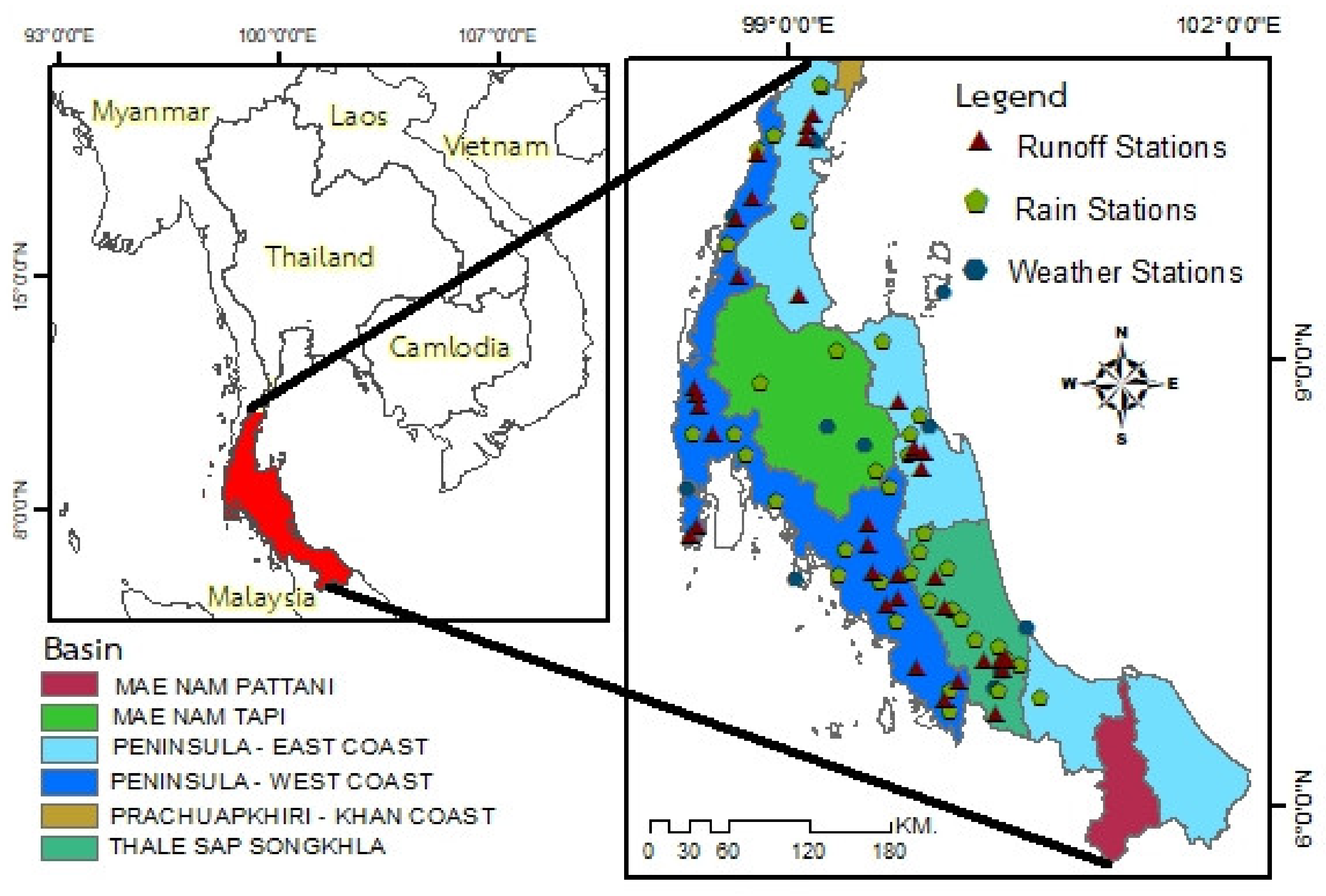
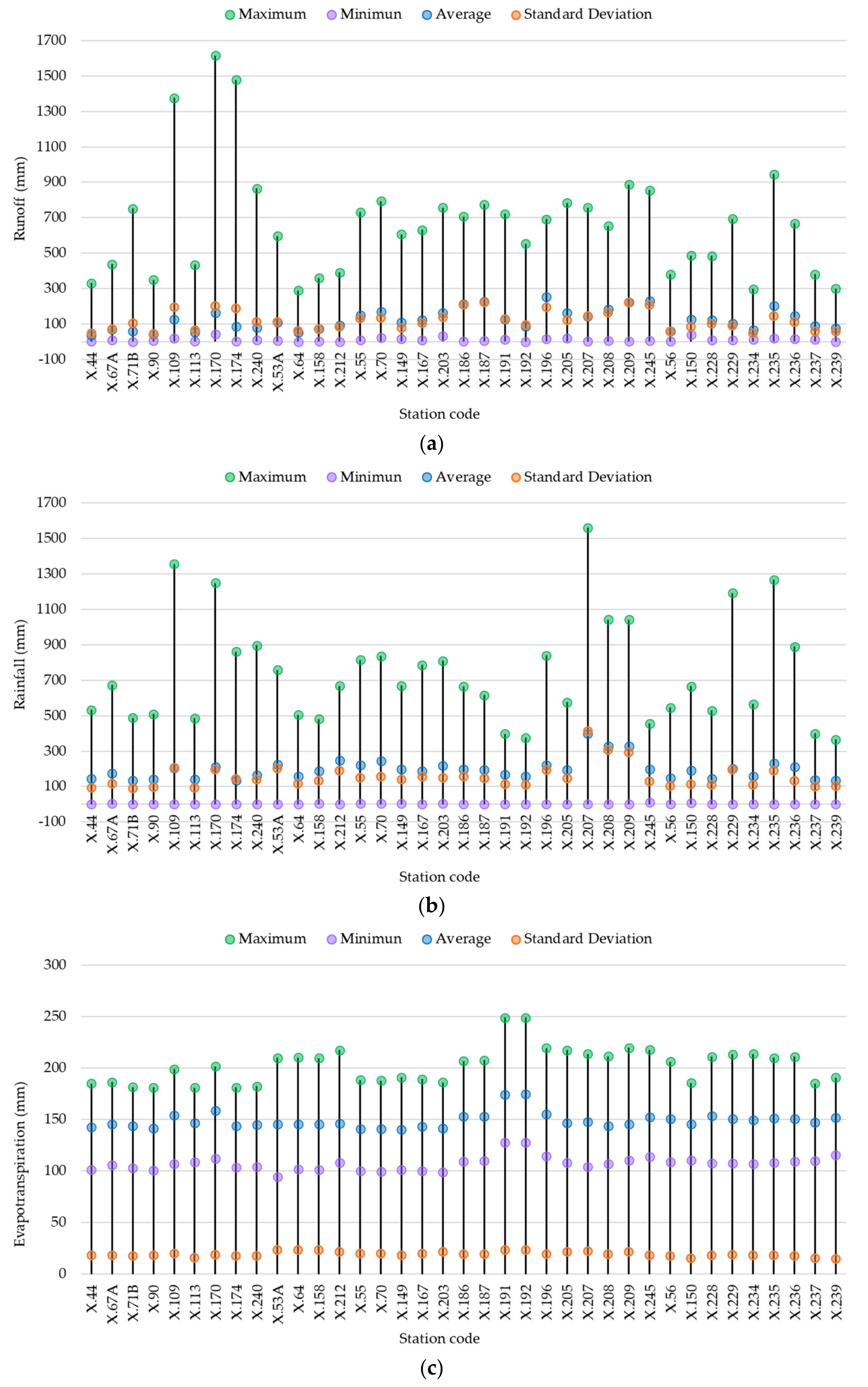
2. Study Area and Data Analysis

This research was conducted in Thailand’s southern basin. It encompasses five major river basins, including the Peninsula-East Coast. Peninsula-West Coast, Mae Nam Tapi, Thale Sap Songkhla, and Mae Nam Pattani, as shown in Figure 1. When investigating monthly rainfall, evapotranspiration, and runoff data, we found only three river basins, i.e., the Peninsula-East Coast, Peninsula-West Coast, Thale Sap Songkhla. Thus, we focused our analysis on these three basins. These river basins have an area of approximately in the range of 13 to 6713 km². Geographically, this portion is the peninsula between the Andaman Sea, which is on the western side, and the South China Sea, which is on the eastern side. The long western mountain range in the northern and central regions also extends to this portion. The Phuket ridge along the west coast and the Nakhon Si Thammarat ridge at the center of the lower portion of the ridge’s southern part is divided into two regions: the east and the west coasts. Climate variability on both sides of the river basins is mainly dominated by the north-eastern monsoon and the south-western monsoon winds. The southwest monsoon wind typically starts in mid-May and ends in mid-October. In contrast, the northeast monsoon typically begins in mid-October and ends in mid-February.

The Peninsula-East Coast watershed covers an area of 26,023.91 km² and encompasses 11 provinces. It also consists of areas covering all parts of Chumphon, Trang, Nakhon Si Thammarat, Narathiwat, Prachuap Khiri Khan, Pattani, Phatthalung, Yala, Ranong, Songkhla, and Surat Thani. The flat coast has a small plain from Chumphon to Narathiwat. Additionally, most rivers are short rivers with approximately 150 km flowing into the Gulf of Thailand. There are nine runoff stations in the Peninsula-East Coast watershed. The Peninsula-West Coast Watershed, 18,841.20 km², consists of seven provinces: Ranong, Phang Nga, Phuket, Krabi, Nakhon Si Thammarat, Trang, and Satun. It also includes Chumphon, Surat Thani, Phatthalung, and Songkhla, with similar topography to the Peninsula-East Coast Watershed. It is a coastal area next to the Andaman Sea. The Phuket Mountains go from Ranong Province to Phang Nga Province, the origin of various rivers and streams. They are generally not long, and they flow mainly to the Andaman Sea in the west and southwest directions. The nineteen runoff stations were used for our analysis. Thale Sap Songkhla watershed, an area of 8484.35 km², primarily covers three provinces, the province of Nakhon Si Thammarat (Some portions of the district of Cha-Uat and the district of Hua Sai), the province of Phatthalung, both provinces, and the province of Songkhla, except for the district of Nathawi, the district of Chana, the district of Thepha and the district of Saba Yoi). Thus, 147 sub-districts and 26 districts, with nine runoff stations, were our study setting. Figure 1 shows the rainfall location, runoff, and weather stations selected in Thailand’s southern basin.

We collected the monthly meteorological and hydrological data from the Royal Irrigation Department (RID) and the Thai Meteorological Department (TMD), including runoff (37 stations), rain (38 stations), and air temperature (13 stations) as shown in the statistical values in Figure 2. We also investigated and analyzed the time corresponding among those three meteorological and hydrological data to select the suitable periods of model’s calibration and verification, as shown in

Table 1. The periods of data used for the GR2M model’s calibration and verification.

No.	Code	Basin Name	Period
			All	Warm-Up	Calibration	Validation
1	X.44	TSS	April 2004–March 2009	April 2004–September 2004	October 2004–February 2007	March 2007–March 2009
2	X.67A	TSS	April 2005–March 2009	April 2005–October 2005	November 2005–September 2007	October 2007–March 2009
3	X.71B	TSS	April 2004–March 2009	April 2004–October 2004	November 2004–April 2007	May 2007–March 2009
4	X.90	TSS	April 2003–March 2009	April 2003–October 2003	November 2003–July 2007	August 2007–March 2009
5	X.109	TSS	April 2003–March 2008	April 2003–October 2003	November 2003–December 2006	January 2007–March 2008
6	X.113	TSS	April 2003–March 2009	April 2003–October 2003	November 2003–November 2006	December 2006–March 2009
7	X.170	TSS	April 2003–March 2009	April 2003–October 2003	November 2003–February 2007	March 2007–March 2009
8	X.174	TSS	April 2003–March 2009	April 2003–October 2003	November 2003–January 2007	February 2007–March 2009
9	X.240	TSS	April 2004–March 2009	April 2004–September 2004	October 2004–February 2007	March 2007–March 2009
10	X.53A	PEC	April 2003–March 2010	April 2003–July 2003	August 2003–December 2006	January 2007–March 2010
11	X.64	PEC	April 2004–March 2009	April 2004–September 2004	October 2004–September 2007	October 2007–March 2009
12	X.158	PEC	April 2004–March 2009	April 2004–August 2004	September 2004–September 2007	October 2007–March 2009
13	X.212	PEC	April 2005–March 2012	April 2005–July 2005	August 2005–June 2009	July 2009–March 2012
14	X.55	PEC	April 2005–March 2009	April 2005–October 2005	November 2005–November 2007	December 2007–March 2009
15	X.70	PEC	April 2005–March 2009	April 2005–September 2005	October 2005–May 2008	June 2008–March 2009
16	X.149	PEC	April 2005–March 2009	April 2005–October 2005	November 2005–April 2008	May 2008–March 2009
17	X.167	PEC	April 2003–March 2009	April 2003–October 2003	November 2003–October 2006	November 2006–March 2009
18	X.203	PEC	April 2005–March 2009	April 2005–October 2005	November 2005–December 2007	January 2008–March 2009
19	X.186	PWC	April 2003–March 2009	April 2003–September 2003	October 2003–December 2006	January 2007–March 2009
20	X.187	PWC	April 2003–March 2009	April 2003–August 2003	September 2003–August 2006	September 2006–March 2009
21	X.191	PWC	April 2003–March 2009	April 2003–August 2003	September 2003–May 2007	June 2007–March 2009
22	X.192	PWC	April 2003–March 2009	April 2003–September 2003	October 2003–August 2006	September 2006–March 2009
23	X.196	PWC	April 2003–March 2009	April 2003–August 2003	September 2003–August 2006	September 2006–March 2009
24	X.205	PWC	April 2005–March 2012	April 2005–August 2005	September 2005–May 2009	June 2009–March 2012
25	X.207	PWC	April 2003–March 2010	April 2003–August 2003	September 2003–September 2007	October 2007–March 2010
26	X.208	PWC	April 2005–March 2009	April 2005–July 2005	August 2005–September 2007	October 2007–March 2009
27	X.209	PWC	April 2005–March 2011	April 2005–July 2005	August 2005–May 2009	June 2009–March 2011
28	X.245	PWC	April 2005–March 2009	April 2005–July 2005	August 2005–June 2007	July 2007–March 2009
29	X.56	PWC	April 2004–March 2009	April 2004–August 2004	September 2004–August 2007	September 2007–March 2009
30	X.150	PWC	April 2005–March 2009	April 2005–September 2005	October 2005–July 2007	August 2007–March 2009
31	X.228	PWC	April 2003–March 2009	April 2003–October 2003	November 2003–September 2006	October 2006–March 2009
32	X.229	PWC	April 2003–March 2009	April 2003–October 2003	November 2003–March 2007	April 2007–March 2009
33	X.234	PWC	April 2004–March 2009	April 2004–September 2004	October 2004–August 2007	September 2007–March 2009
34	X.235	PWC	April 2004–March 2009	April 2004–September 2004	October 2004–September 2007	October 2007–March 2009
35	X.236	PWC	April 2004–March 2009	April 2004–July 2004	August 2004–December 2006	January 2007–March 2009
36	X.237	PWC	April 2004–March 2009	April 2004–August 2004	September 2004–January 2007	February 2007–March 2009
37	X.239	PWC	April 2004–March 2009	April 2004–July 2004	August 2004–December 2007	January 2007–March 2009

Remark: TSS = Thale Sap Songkhla; PWC = Peninsular-West Coast; PEC = Peninsular-East Coast.

. The Thiessen polygon was used to determine the mean areal precipitation in the considered basin from rain gauge observations. The monthly evapotranspiration, which is one of the input data for the GR2M model, was calculated from the average monthly air temperature (Ti) data by Thornthwaite [24], as shown below:

• Monthly values of the heat index

  $${\mathrm{I}}_{\mathrm{i}}={\left(\frac{{\mathrm{T}}_{\mathrm{i}}}{5}\right)}^{1.514}$$

  (1)
• Annual temperature efficiency index

  $$\mathrm{J}={\displaystyle \sum }_{\mathrm{i}=1}^{12}\left({\mathrm{I}}_{\mathrm{i}}\right)$$

  (2)
• Evapotranspiration

  $${\mathrm{PET}}_{\mathrm{i}}\left(0\right)=1.6{\left(\frac{10{\mathrm{T}}_{\mathrm{i}}}{\mathrm{J}}\right)}^{\mathrm{C}}$$

  (3)
• The C value can be obtained from:

  $$\mathrm{C}=0.000000675{\mathrm{J}}^3-0.0000771{\mathrm{J}}^2+0.01792\mathrm{J}+0.49239$$

  (4)
• Potential Evapotranspiration

  $${\mathrm{PET}}_{\mathrm{i}}\left(\mathrm{L}\right) = \mathrm{K}\times {\mathrm{PET}}_{\mathrm{i}}\left(0\right)$$

  (5)

  where ${\mathrm{T}}_{\mathrm{i}}$ = Monthly average temperature (°C), $\mathrm{K}$ = PET constants at different latitudes.

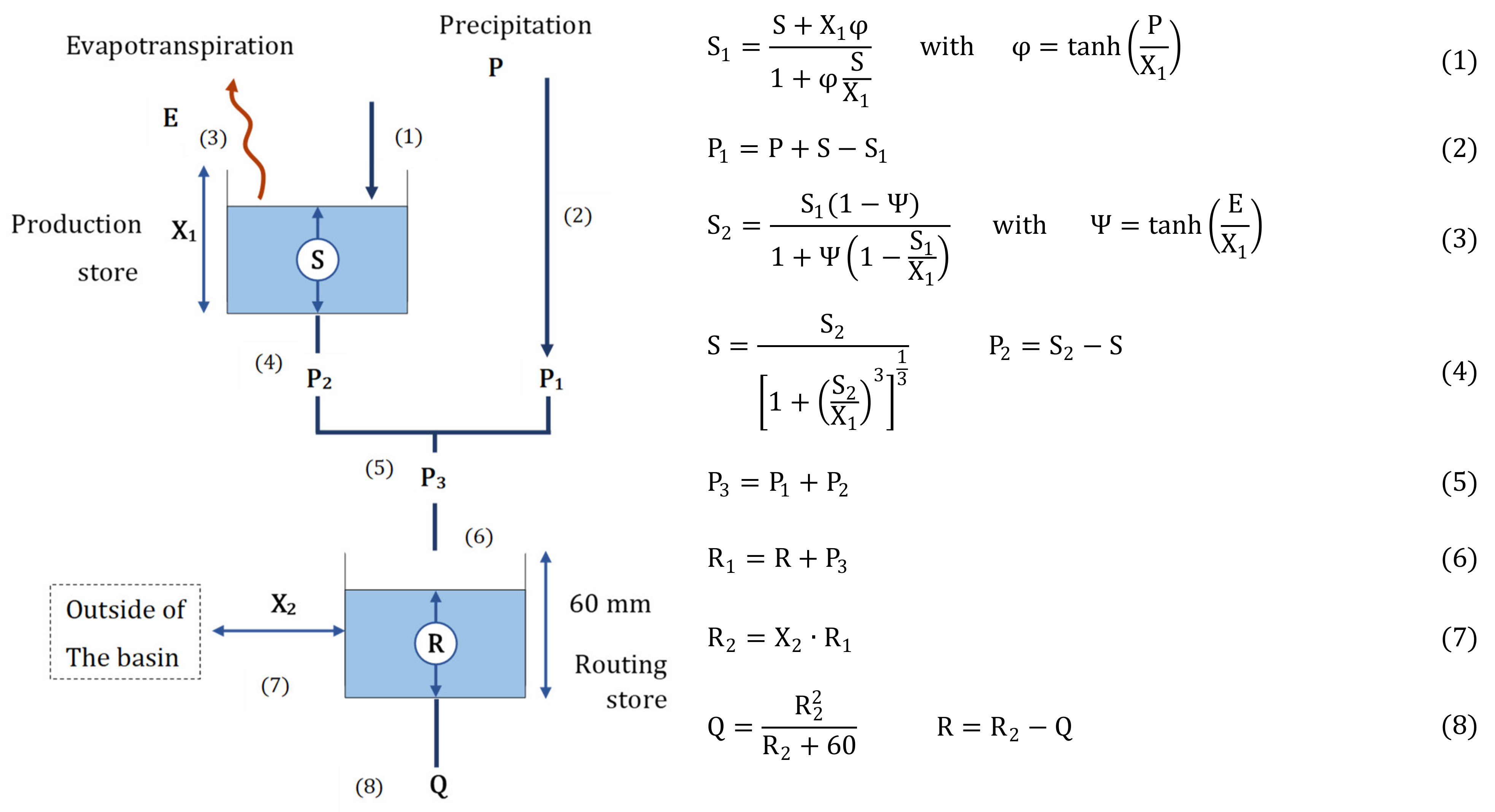
3. GR2M Model

The GR2M, a conceptual model, was first introduced by Demagref in the late 1980s and it has been widely applied for water resources management [25]. The model aims to simulate the relationship between monthly rainfall and runoff and reproduce the hydrological system’s response. It has been continuously being developed to improve its efficiency by Kabouya [26], Makhlouf and Michel [27], Mouelhi [28] until Mouelhi et al. [29]. The model selected in this study was the latest version, GR2M 2006. It is the most popular and efficient compared to other models [13]. The GR2M model’s advantage requires only two parameters: production store: X₁ (mm) and groundwater exchange rate (X₂). Additionally, it needs only three monthly meteorological and hydrological data, i.e., rainfall, runoff, and evapotranspiration [30,31]. The GR2M model results give runoff hydrograph and other elements such as soil moisture content, surface runoff, the groundwater flow.

The structure of the GR2M model consisted of two reservoirs, as presented in Figure 3. The first reservoir represents soil moisture (S) of the basin-controlled production store: X₁ (mm). Furthermore, the second reservoir is water flow through the river (R). Its capacity is up to 60 mm and is regulated by the groundwater exchange rate (X₂). This model starts with the precipitation infiltrated into the soil, causes soil moisture at the level: S₁ (mm). When the soil reaches a saturation point, the remnants of infiltration rain become rainfall excess: P₁ (mm). The soil moisture loss from evapotranspiration: E until the remaining moisture level: S₂ (mm).

Additionally, some moisture content is released as surface water: P₂ (mm) and gradually released with rainfall excess. This water section is called surface runoff or net rainfall: P3 (mm), which moved into the flow path combined with the remaining water from the initial or existing water in the river: R (mm). It causes the water content at level R1 (mm). The water volume movement may change because some water may be lost, causing the residual water volume at the level: R₂ (mm). Ultimately, the total amount of water discharge into the runoff streamflow gauging station conducted the assessment.

4. Model’s Calibration and Verification

In achieving our aims in evaluating a Two-Parameters Monthly Rainfall-Runoff Model’s performance, the GR2M model applied in Thailand’s southern basin was calibrated and verified. It included two steps, i.e., the warm-up period and calibrating and verifying the GR2M Model.

4.1. Warm-Up Period

In this process, the appropriate initial parameters of X₁ and X₂ are determined. It enables the model to mimic the basin’s existing hydrological behavior at the considered runoff stations before conducting the model’s calibration and verification. The R-value, the initial or existing water capacity in the river, is varied between 10 mm and 60 mm to determine the suitable warm-up period. In our study, we found the warm-up periods of approximately 4 to 7 months.

4.2. Calibrating and Verifying the GR2M Model

As widely known, the calibration and verification processes are imperative for applying the mathematical model to find the most suitable model’s parameters. The model can simulate the behavior of our concerning water system. For the GR2M model, only two parameters: the production store (X₁) and the groundwater exchange rate (X₂), must be calibrated and validated. Microsoft Excel solvers help by giving an objective function and practical constraints, which can automatically solve the fair values of X₁ and X₂ parameters for each runoff station. The GR2M model was calibrated and verified for 37 different runoff stations in the Southern Basins in this study. The details of the intervals for the calibration and verification of the model are presented in Table 1. The lowest and the highest periods used for running the GR2M model are 41 and 80 months. The used range of the calibration and verification periods consists of 22 and 48, and 10 and 39 months, respectively.

5. Performance Criteria for Evaluating the Applicability of the GR2M Model

In this study, three performance criteria were used for evaluating the performance and applicability of the GR2M Model. They included Nash–Sutcliffe Efficiency (NSE), Correlation Coefficient (r), and Overall Index (OI). The details for each performance criteria can be delineated as shown the following:

Nash-Sutcliffe Efficiency (NSE) [32] is a popular index used to tell model accuracy or efficiency-effectiveness of the model (Model Performance) in estimating the desired value. As the equation below:

$$\mathrm{NSE}=1-\frac{{{\displaystyle \sum }}_{\mathrm{i}=1}^{\mathrm{n}}{\left({\mathrm{Q}}_{\mathrm{cal}}-{\mathrm{Q}}_{\mathrm{obs}}\right)}^2}{{{\displaystyle \sum }}_{\mathrm{i}=1}^{\mathrm{n}}{\left({\mathrm{Q}}_{\mathrm{obs}}-{\acute{\mathrm{Q}}}_{\mathrm{obs}}\right)}^2}$$

(6)

NSE is between −∞ to 1. Suppose the Nash values are close to 1. In that case, the model results and the measurement results are similar. They are considered the model of efficiency or accuracy in forecasting [33].

Correlation Coefficient (r) is a simple linear regression equation. It is a simple linear regression equation that can be used to estimate the Y as well. If X and Y are correlated well. The correlation coefficient between X and Y can be calculated from the following equation.

$$\mathrm{r}=\frac{{{\displaystyle \sum }}_{\mathrm{i}=1}^{\mathrm{n}}\left({\mathrm{Q}}_{\mathrm{obs}}-{\overline{\mathrm{Q}}}_{\mathrm{obs}}\right)\left({\mathrm{Q}}_{\mathrm{cal}}-{\overline{\mathrm{Q}}}_{\mathrm{cal}}\right)}{\sqrt{{{\displaystyle \sum }}_{\mathrm{i}=1}^{\mathrm{n}}{({\mathrm{Q}}_{\mathrm{obs}}-{\overline{\mathrm{Q}}}_{\mathrm{obs}})}^2}\cdot \sqrt{{{\displaystyle \sum }}_{\mathrm{i}=1}^{\mathrm{n}}{({\mathrm{Q}}_{\mathrm{cal}}-{\overline{\mathrm{Q}}}_{\mathrm{cal}})}^2}}$$

(7)

The r-value is between −1 and 1. The squares of r or R2 will always be between 0–1, and in this sense, if R2 is 0, then the two variables have no linear correlation. If R2 is equal to 1, then there is an entirely linear correlation. If the r-value approaches 1, the model results and the measurement results are related. The plus sign (+) or minus sign can also tell the direction of the data set’s relationship. The plus sign (+) means the dataset is related. Suppose the data obtained from the model is precious. The data obtained from the measurement is also precious. The minus sign (−) means the dataset is in the opposite relationship. If the information is valuable More information will be less [34,35,36].

Overall Index:

$$\mathrm{OI}=\frac{1}{2} \left[2-\frac{\mathrm{RMSE}}{{\mathrm{Q}}_{\mathrm{obs},\max }-{\mathrm{Q}}_{\mathrm{obs},\min }}-\frac{{{\displaystyle \sum }}_{\mathrm{i}=1}^{\mathrm{n}}{\left({\mathrm{Q}}_{\mathrm{obs}}-{\mathrm{Q}}_{\mathrm{cal}}\right)}^2}{{{\displaystyle \sum }}_{\mathrm{i}=1}^{\mathrm{n}}{\left({\mathrm{Q}}_{\mathrm{obs}}-{\overline{\mathrm{Q}}}_{\mathrm{obs}}\right)}^2}\right]$$

(8)

The OI value is a criterion that indicates model performance. It is between −∞ to 1. If the higher OI is closer to 1, the model’s performance is favorable [37,38]. where; ${\mathrm{Q}}_{\mathrm{obs}}$ is the amount of runoff obtained from the measurement, ${\mathrm{Q}}_{\mathrm{cal}}$ is the amount of runoff obtained from the calculation, ${\overline{\mathrm{Q}}}_{\mathrm{obs}}$ is the average runoff from the measure, ${\overline{\mathrm{Q}}}_{\mathrm{cal}}$ is the average runoff from the calculation, ${\mathrm{Q}}_{\mathrm{obs},\max }$ is the runoff from the highest measurement ${\mathrm{Q}}_{\mathrm{obs},\min }$ is the runoff from the lowest measurements, and n is the amount of information.

6. Results and Discussion

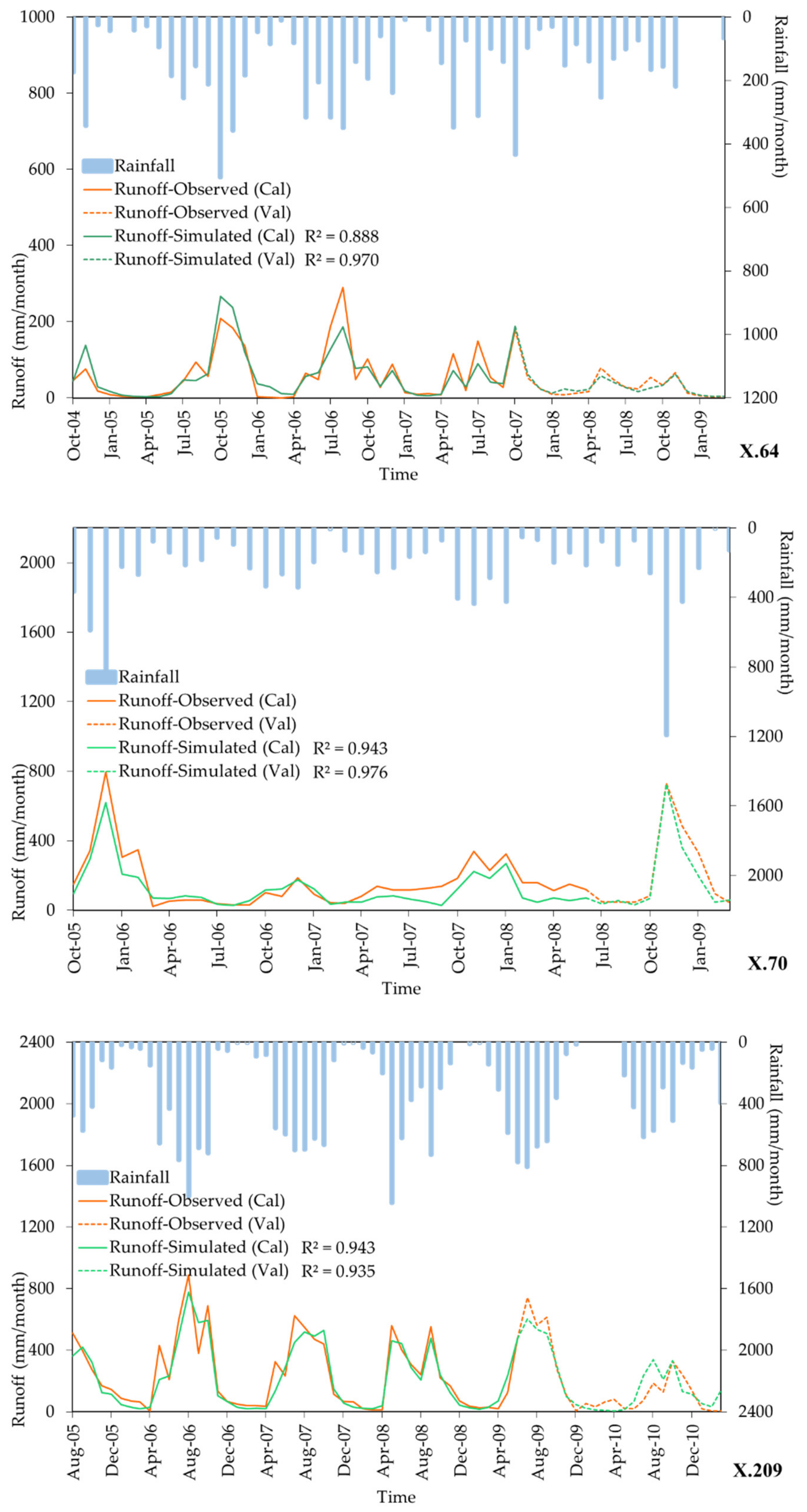
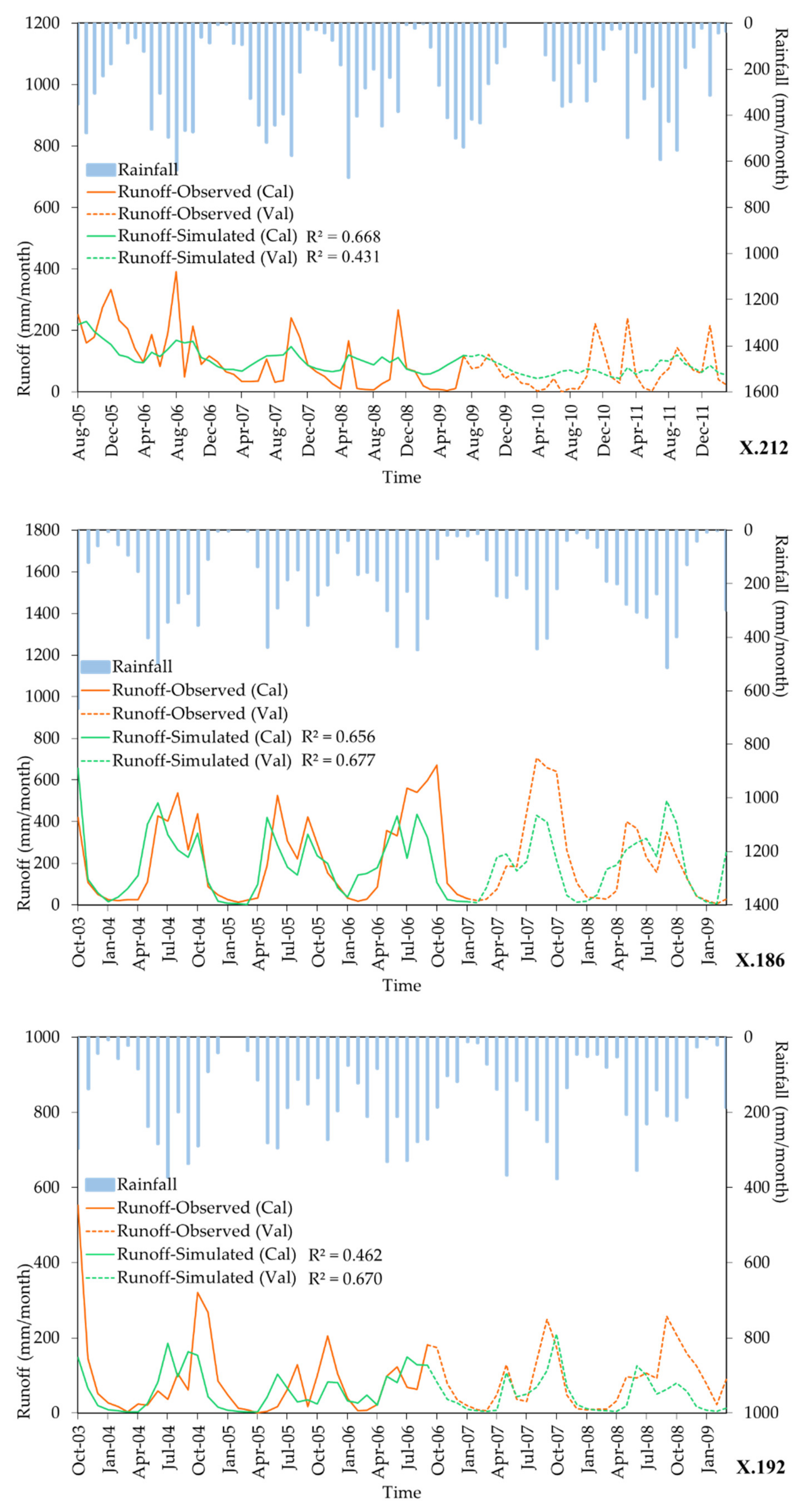
6.1. The Results of Calibrating and Verifying the GR2M Model

Table 2. Results of calibrating and verifying the GR2M model.

No.	Code	Performance Criteria						No.	Code	Performance Criteria
		Calibration			Validation					Calibration			Validation
		NSE	r	OI	NSE	r	OI			NSE	r	OI	NSE	r	OI
1	X.44	0.942	0.973	0.949	0.465	0.705	0.657	20	X.187	0.563	0.756	0.668	0.349	0.654	0.548
2	X.67A	0.978	0.99	0.974	0.719	0.852	0.795	21	X.191	0.177	0.492	0.505	0.664	0.831	0.749
3	X.71B	0.688	0.954	0.793	0.605	0.797	0.733	22	X.192 b	0.165	0.462	0.493	0.167	0.670	0.451
4	X.90	0.772	0.887	0.85	0.468	0.502	0.478	23	X.196	0.333	0.691	0.544	0.283	0.691	0.505
5	X.109	0.925	0.987	0.94	0.577	0.849	0.696	24	X.205 c	0.518	0.755	0.693	−0.119	0.663	0.289
6	X.113	0.736	0.91	0.821	0.479	0.796	0.648	25	X.207	0.758	0.878	0.798	0.836	0.920	0.856
7	X.170	0.805	0.903	0.867	0.038	0.451	0.392	26	X.208	0.796	0.906	0.838	0.751	0.894	0.808
8	X.174	0.725	0.975	0.821	0.385	0.731	0.61	27	X.209 a	0.880	0.943	0.896	0.870	0.935	0.883
9	X.240	0.975	0.993	0.973	0.511	0.735	0.687	28	X.245	0.476	0.715	0.636	0.199	0.503	0.457
10	X.53A	0.822	0.908	0.868	0.714	0.847	0.793	29	X.56	0.813	0.911	0.868	0.676	0.866	0.746
11	X.64 a	0.787	0.888	0.838	0.941	0.970	0.942	30	X.150	0.833	0.915	0.871	0.226	0.623	0.461
12	X.158	0.573	0.759	0.714	0.752	0.869	0.818	31	X.228	0.111	0.527	0.450	0.346	0.702	0.554
13	X.212 b	0.383	0.668	0.594	0.173	0.431	0.467	32	X.229 c	0.564	0.794	0.730	−0.437	0.407	0.120
14	X.55	0.654	0.903	0.761	0.987	0.996	0.980	33	X.234	0.854	0.934	0.890	0.713	0.882	0.773
15	X.70 a	0.780	0.943	0.845	0.923	0.976	0.916	34	X.235	0.430	0.758	0.648	0.404	0.679	0.596
16	X.149	0.557	0.912	0.702	0.957	0.986	0.950	35	X.236	0.801	0.896	0.857	0.513	0.719	0.647
17	X.167	0.892	0.973	0.912	0.278	0.803	0.534	36	X.237 c	0.734	0.277	0.411	−0.305	0.497	0.202
18	X.203	0.732	0.970	0.809	0.897	0.973	0.904	37	X.239	0.376	0.754	0.602	0.055	0.673	0.388
19	X.186 b	0.400	0.660	0.580	0.405	0.680	0.620
Maximum										0.978	0.993	0.974	0.987	0.996	0.980
Minimum										0.111	0.277	0.411	−0.437	0.407	0.120
Average										0.657	0.825	0.757	0.472	0.750	0.639
Standard Deviation										0.233	0.170	0.153	0.350	0.166	0.213

Remark: TSS = Thale Sap Songkhla; PWC = Peninsular-West Coast; PEC = Peninsular-East Coast. ^a the green text shows the best top-three model performance stations, ^b the red text shows the worst top-three model performance stations, ^c the blue text shows stations having the overfitting models.

shows the results of the model’s calibration and verification. It explicitly indicated that the GR2M model could be applied for modeling monthly rainfall-runoff in the southern region of Thailand.

The average performance criteria gave NSE, r, and OI values for the calibration stage of 0.657, 0.825, and 0.757. Those values for the verification stage of 0.472, 0.750, and 0.639, respectively. Lian, et al. [39] suggested that the model had a good prediction since NSE was in the range of 0.36 to 0.75. By obtaining an r-value of more than 0.70, it indicated a strong positive linear relationship between simulated and observed runoff [36]. Moreover, the OI value of more than 0.60 showed the model had relatively high forecasting accuracy. The three performance criteria previously mentioned emphasized a strong consistency between the runoff data obtained from the measurements and model-simulated for our study.

Considering the best top-three model performance stations obtaining from X.64, X.70, and X.209, NSE, r, and OI values for both calibration and verification processes gave more than 0.76, it showed the GR2M model performed quite satisfactorily for simulating monthly runoff. Conversely, the worst top-three model performance stations were X.212, X.186, and X.192. They gave NSE, r, and OI values for both calibration and verification processes less than 0.690. However, some runoff stations, i.e., X.205, X.229, and X.237, had a negative NSE value. It represented overfitting models for those three runoff stations and could not be generally applied. Although many attempts were being made for the model’s calibration and verification processes, the quality and accuracy of measured hydrological and meteorological data are the most important things to concern and check the consistency. Figure 4 illustrates the relationship between rainfall and runoff obtained from running the GR2M model. Herein present six examples of runoff stations, i.e., X.64, X.70, X.209, X.212, X186, and X.192. The best top-three and the worst top-three model performance stations are presented.

Likewise, the bar chart in blue represents rainfall time-series variation. The line graphs in orange and green also show the observed and simulated runoff time-series variation, respectively. For both runoff time-series variations, the solid and dot lines mean calibration and validation periods, respectively. A slight difference runoff time-series value was observed for the best top-three model performance stations. A significant difference was observed among runoff time-series values for the worst top-three model performance stations. However, both cases underestimated runoff value; that is, the simulated runoff was lower than the observed runoff. It could realize when using the calibrated and verified GR2M model, especially for water resources management and planning for rainy and dry seasons.

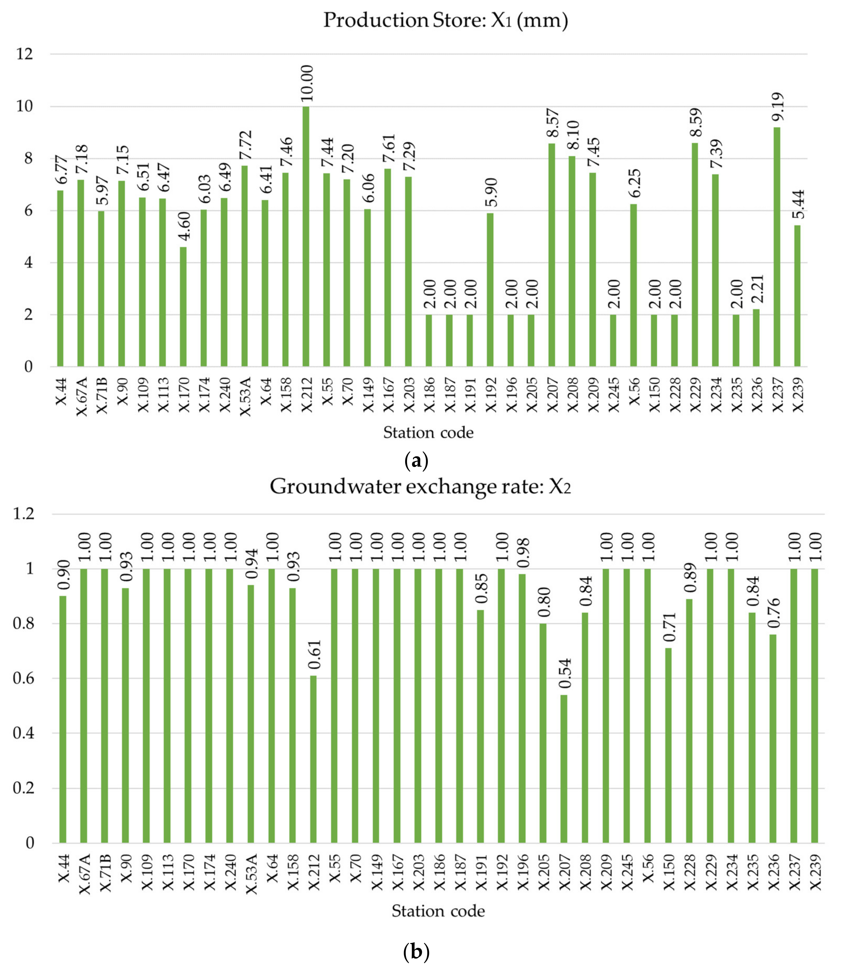
6.2. The Optimal Values of Production Store Capacity (X₁) and Groundwater Exchange Rate (X₂)

Figure 5 shows suitable X₁ and X₂ parameters of the GR2M model for each runoff station obtained from the model’s calibration and verification.

The production store (X₁) value results ranged from 2.00 mm to 10.00 mm. It showed a spatial variation of X₁ value, and its values ranged from the minimum (2.00 mm) and maximum (10.00 mm) values. The average and standard deviation values of X₁ were 5.71 mm, and 2.49 mm, respectively. Furthermore, the skewness and kurtosis values of X₁ were −0.52 and −1.03, respectively. It could physically explain river basin characteristics in terms of production store (X₁). It had left skew, platykurtic, and non-symmetric distributions. The groundwater exchange rate (X₂) value results ranged from 0.54 to 1.00. Those X₂ values mostly reached the maximum value (1.00). The average and standard deviation values of X₂ were 0.93 and 0.12, respectively. Moreover, the skewness and kurtosis values of X₂ were −2.01 and 3.69, respectively. It could physically explain river basin characteristics in terms of the groundwater exchange rate (X₂). It had left skew, leptokurtic, and non-symmetric distributions. The positive value of groundwater exchange rate (X₂) displayed no groundwater flows outside the basin.

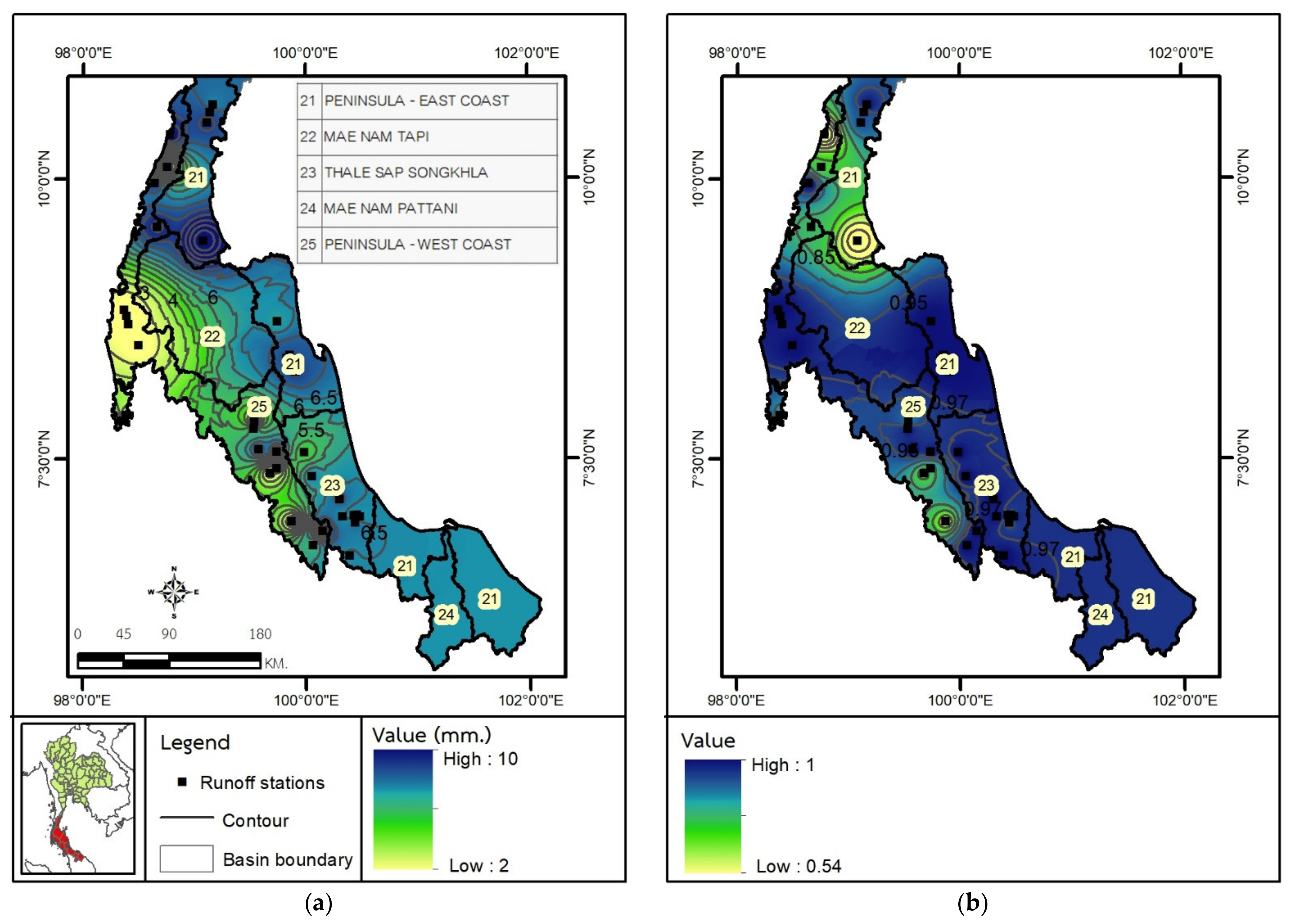
6.3. The Spatial Distribution of X₁ and X₂ Values Using the Inverse Distance Weighting (IDW) Method

Figure 6 shows the spatial distribution of X₁ and X₂ values using the IDW method. As seen from Figure 5a, the low production store (X₁) value (yellow and green color) was generally located on the Peninsular-West Coast. The significant area roughly was covered by the average production store (X₁) value (5.71 mm). Most areas were a light blue color. Only the northern part of Surat Thani province shows the high production store (X₁) value, which shows the dark blue zone. For the groundwater exchange rate (X₂), as depicted in Figure 5b, most areas were governed by the dark blue zone. It indicated that most areas in the southern basin, Thailand, had a high groundwater exchange rate (X₂).

Furthermore, it agreed to the average X₂ value of 0.93. The northern part of Surat Thani province and some Chumporn, Trang, and Satun provinces show the low groundwater exchange rate (X₂) value, as portrayed in the yellow and green zone. Suppose we do not have a measured gauged or ungauged. In that case, we can use these figures to determine the values of X₁ and X₂ roughly. If we know areal rainfall and evaporation, we can also estimate the runoff via the GR2M model.

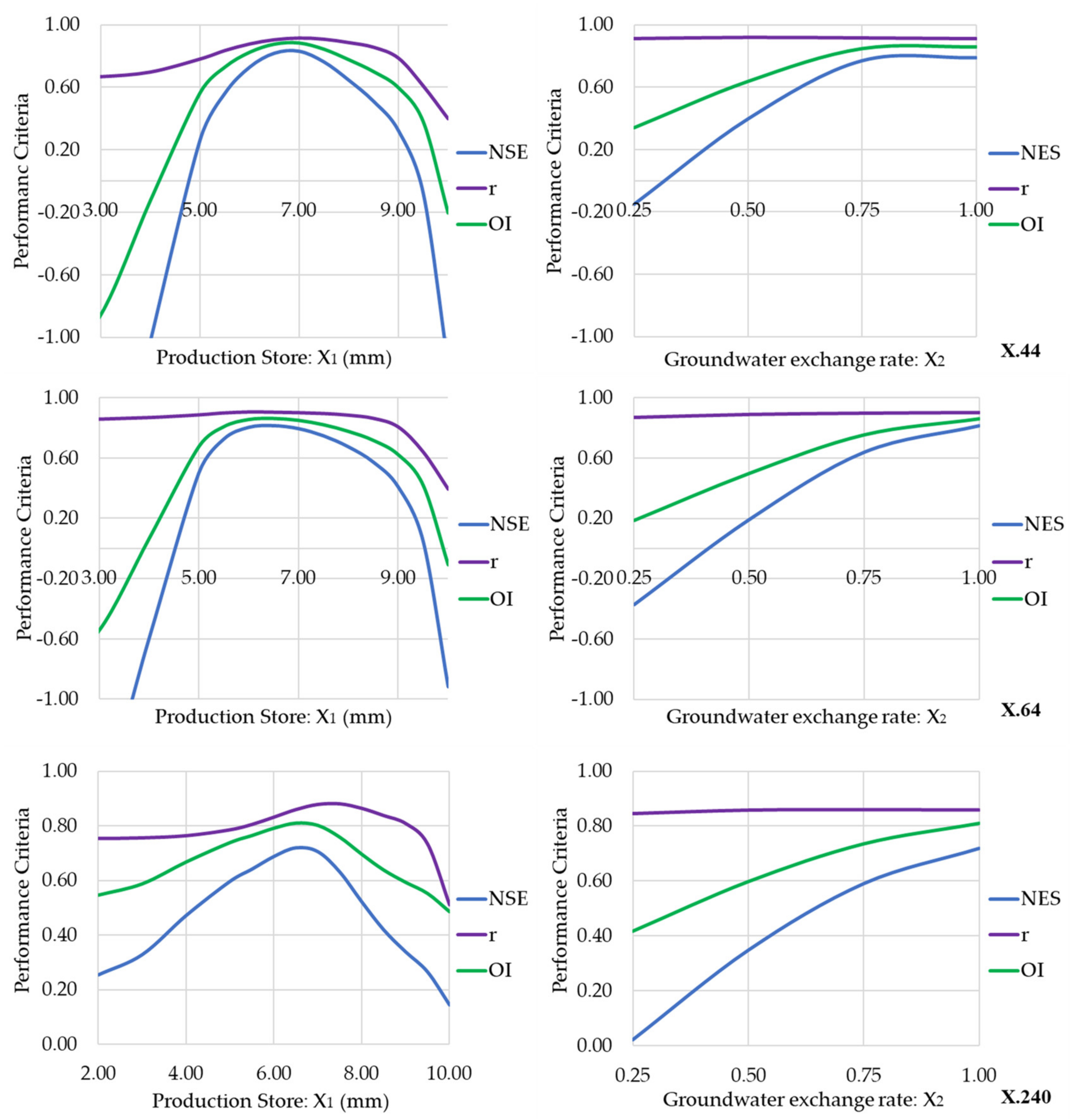
7. Sensitivity Analysis

The sensitivity analysis [10] was conducted in this study to understand the effects of the two model parameters (i.e., X₁ and X₂). We randomly selected three runoff stations (X.44, X.64, and X.240) as the representative for all 37 runoff stations due to the analysis sensitivity. By fixing the optimal X₂ value obtained from calibration and verification stages and then varying the X₁ value in it ranges from the minimum to maximum (2 mm to 10 mm) [31,36], we received the results of X₁’s sensitivity analysis. Similarly, by fixing the optimal X₁ value obtained from calibration and verification stages and then varying the X₁ value in it ranges from the minimum to maximum (−1 to 1) [31,34], we got the results of X₂’s sensitivity analysis. It was rarely reported about the sensitivity analysis for the GR2M model’s two parameters to our best knowledge. Thus, it was the early attempt to conduct their sensitivity analysis. As evidentially presented in Figure 7, the X₁ value was sensitive. Apart from the optimal value obtained from the calibration and verification stages, the other value gave a lower model’s performance. Considering the X₂ value, we found that the higher value (approximately more than 0.90) was trial, it gave the higher model’s performance. It also confirmed and corresponded with the results, as found in Figure 5 and Figure 6.

Rainfall-runoff modeling is among the most challenging task for hydrologists, particularly in regions with scarce rainfall and runoff data records. The complexity of the rainfall-runoff modeling also comes from the non-stationary features of its components, such as seasonality, potential trend, and the non-linear behavior of the variables involved in the modeling process [11,40]. Geomorphological features characterizing the watershed influence significantly the runoff regime; namely, in urban areas, high imperviousness areas cause increased runoff by originating floods while the same behavior is not observed in fewer imperviousness areas [1,3]. Thus, it is crucial to know the sensitivity of parameters in the rainfall-runoff modeling, especially in the urban areas, making the calibration process more efficient by focusing only on the parameters for which the modeling results are more sensitive [10]. The findings resulted from this study contribute to enhance the understanding of the hydrological parameters and processes that govern a watershed system. Also, it offers new insights on the application of the GR2M model in regions characterized by a similar climate and geomorphological conditions to support decision-makers and optimize the planning and operation rules of water resources systems [21,40]. Last, for areas, especially large basins suffering from a lack of hydrometeorological data records it is important to assess the areal inhomogeneity of the investigated gauging station network [41,42]. In that regard, knowing the fractal dimension of the hydrometeorological network and its limits of validity is the key to understanding the limits of reliability of an inhomogeneous distribution of gauging stations [42].

8. Conclusions

With only two parameters, namely, the production store (X₁) and the groundwater exchange rate (X₂), our research work explicitly indicated GR2M model could be applied for modeling monthly rainfall-runoff in the southern region of Thailand. The model’s calibration results for 37 runoff stations gave the average NSE, r, and OI of 0.657, 0.825, and 0.757. Those values for verification of 0.472, 0.750, and 0.639, respectively. The range of X₁ was between 2.00 and 10.00, and the range of X₂ was between 0.54 and 1.00. It was sensitive to the X₁ value. The other value indicates lower model efficiency, apart from the optimum value obtained from the calibration and verification phases. We also found that the higher value of X₂ (approximately more than 0.90) gave the higher model’s performance. Personnel concerning water resources planning and management can apply our work for a guideline for utilizing the GR2M model to determine monthly runoff in other runoff stations located in the southern region, Thailand. It is because there are similar hydrological, geological, and topological basin characteristics. However, to further enhance the GR2M model’s reliability, a more extended period of recorded hydrological data is required. Also, more runoff gauging station installation will cover the variety of existing watershed characteristics.

References

1. Vaze, J.; Chiew, F.; Perraud, J.; Viney, N.; Post, D.; Teng, J.; Wang, B.; Lerat, J.; Goswami, M. Rainfall-runoff Modelling across Southeast Australia: Datasets, Models and Results. Australas. J. Water Resour. 2010, 14, 101–116. [Google Scholar] [CrossRef]
2. Suwal, N.; Kuriqi, A.; Huang, X.; Delgado, J.; Młyński, D.; Walega, A. Environmental Flows Assessment in Nepal: The Case of Kaligandaki River. Sustainability 2020, 12, 8766. [Google Scholar] [CrossRef]
3. Ahmad, M.-U.-D.; Peña-Arancibia, J.L.; Stewart, J.P.; Kirby, J.M. Water balance trends in irrigated canal commands and its implications for sustainable water management in Pakistan: Evidence from 1981 to 2012. Agric. Water Manag. 2021, 245, 106648. [Google Scholar] [CrossRef]
4. López-Lambraño, A.; Martínez-Acosta, L.; Gámez-Balmaceda, E.; Medrano-Barboza, J.; López, J.R.; López-Ramos, A. Supply and Demand Analysis of Water Resources. Case Study: Irrigation Water Demand in a Semi-Arid Zone in Mexico. Agriculture 2020, 10, 333. [Google Scholar] [CrossRef]
5. Zhang, X.; Guo, P.; Zhang, F.; Liu, X.; Yue, Q.; Wang, Y. Optimal irrigation water allocation in Hetao Irrigation District con-sidering decision makers’ preference under uncertainties. Agric. Water Manag. 2021, 246, 106670. [Google Scholar] [CrossRef]
6. Chen, Q.; Chen, H.; Wang, J.; Zhao, Y.; Chen, J.; Xu, C. Impacts of Climate Change and Land-Use Change on Hydrological Extremes in the Jinsha River Basin. Water 2019, 11, 1398. [Google Scholar] [CrossRef] [Green Version]
7. Kabiri, R.; Bai, V.R.; Chan, A. Assessment of hydrologic impacts of climate change on the runoff trend in Klang Watershed, Malaysia. Environ. Earth Sci. 2015, 73, 27–37. [Google Scholar] [CrossRef]
8. Lin, B.; Chen, X.; Yao, H.; Chen, Y.; Liu, M.; Gao, L.; James, A. Analyses of landuse change impacts on catchment runoff using different time indicators based on SWAT model. Ecol. Indic. 2015, 58, 55–63. [Google Scholar] [CrossRef]
9. Kwak, J.; Lee, J.; Jung, J.; Kim, H.S. Case Study: Reconstruction of Runoff Series of Hydrological Stations in the Nakdong River, Korea. Water 2020, 12, 3461. [Google Scholar] [CrossRef]
10. Ballinas-González, H.A.; Alcocer-Yamanaka, V.H.; Canto-Rios, J.J.; Simuta-Champo, R. Sensitivity Analysis of the Rainfall–Runoff Modeling Parameters in Data-Scarce Urban Catchment. Hydrology 2020, 7, 73. [Google Scholar] [CrossRef]
11. Lerat, J.; Thyer, M.; McInerney, D.; Kavetski, D.; Woldemeskel, F.; Pickett-Heaps, C.; Shin, D.; Feikema, P. A robust approach for calibrating a daily rainfall-runoff model to monthly streamflow data. J. Hydrol. 2020, 591, 125129. [Google Scholar] [CrossRef]
12. Abdessamed, D.; Abderrazak, B. Coupling HEC-RAS and HEC-HMS in rainfall–runoff modeling and evaluating floodplain inundation maps in arid environments: Case study of Ain Sefra city, Ksour Mountain. SW of Algeria. Environ. Earth Sci. 2019, 78, 586. [Google Scholar] [CrossRef]
13. Zhang, C.; Wang, R.-B.; Meng, Q.-X. Calibration of Conceptual Rainfall-Runoff Models Using Global Optimization. Adv. Meteorol. 2015, 2015, 545376. [Google Scholar] [CrossRef]
14. Khazaei, M.R.; Zahabiyoun, B.; Saghafian, B.; Ahmadi, S. Development of an Automatic Calibration Tool Using Genetic Algorithm for the ARNO Conceptual Rainfall-Runoff Model. Arab. J. Sci. Eng. 2013, 39, 2535–2549. [Google Scholar] [CrossRef]
15. Dezetter, A.; Girard, S.; Paturel, J.; Mahé, G.; Ardoin-Bardin, S.; Servat, E. Simulation of runoff in West Africa: Is there a single data-model combination that produces the best simulation results? J. Hydrol. 2008, 354, 203–212. [Google Scholar] [CrossRef]
16. Okkan, U.; Fistikoglu, O. Evaluating climate change effects on runoff by statistical downscaling and hydrological model GR2M. Theor. Appl. Clim. 2014, 117, 343–361. [Google Scholar] [CrossRef]
17. Lyon, S.W.; King, K.; Polpanich, O.-U.; Lacombe, G. Assessing hydrologic changes across the Lower Mekong Basin. J. Hydrol. Reg. Stud. 2017, 12, 303–314. [Google Scholar] [CrossRef]
18. Zamoum, S.; Souag-Gamane, D. Monthly streamflow estimation in ungauged catchments of northern Algeria using regional-ization of conceptual model parameters. Arab. J. Geosci. 2019, 12, 342. [Google Scholar] [CrossRef]
19. Boulariah, O.; Longobardi, A.; Meddi, M. Statistical comparison of nonlinear rainfall-runoff models for simulation in Africa North-West semi-arid areas. In Proceedings of the 15th International Conference on Environment Science and Technology, Rhodes, Greece, 31 August–2 September 2017. [Google Scholar]
20. Topalović, Ž.; Todorović, A.; Plavšić, J. Evaluating the transferability of monthly water balance models under changing climate conditions. Hydrol. Sci. J. 2020, 65, 928–950. [Google Scholar] [CrossRef]
21. Hadour, A.; Mahé, G.; Meddi, M. Watershed based hydrological evolution under climate change effect: An example from North Western Algeria. J. Hydrol. Reg. Stud. 2020, 28, 100671. [Google Scholar] [CrossRef]
22. Rintis, H.; Suyanto; Setyoasri, Y.P. Rainfall-Discharge Simulation in Bah Bolon Catchment Area by Mock Method, NRECA Method, and GR2M Method. Appl. Mech. Mater. 2016, 845, 24–29. [Google Scholar] [CrossRef]
23. O’Connor, P.; Murphy, C.; Matthews, T.; Wilby, R.L. Reconstructed monthly river flows for Irish catchments 1766–2016. Geosci. Data J. 2020, 1766–2016. [Google Scholar] [CrossRef]
24. Thornthwaite, C.W. An approach toward a rational classification of climate. Geogr. Rev. 1948, 38, 55–94. [Google Scholar] [CrossRef]
25. Paturel, J.E.; Servat, E.; Vassiliadis, A. Sensitivity of conceptual rainfall-runoff algorithms to errors in input data—Case of the GR2M model. J. Hydrol. 1995, 168, 111–125. [Google Scholar] [CrossRef]
26. Kabouya, M. Modélisation Pluie-Débit aux Pas de Temps Mensuel et Annuel en Algérie Septentrionale. Ph.D. Thesis, Université Paris Sud Orsay, Orsay, France, 1990. [Google Scholar]
27. Makhlouf, Z.; Michel, C. A two-parameter monthly water balance model for French watersheds. J. Hydrol. 1994, 162, 299–318. [Google Scholar] [CrossRef]
28. Mouelhi, S. Vers Une Chaîne Cohérente de Modèles Pluie-Débit Conceptuels Globaux aux Pas de Temps Pluriannuel, Annuel, Mensuel et Journalier. Ph.D. Thesis, ENGREF Paris, Paris, France, 2003. [Google Scholar]
29. Mouelhi, S.; Michel, C.; Perrin, C.; Andréassian, V. Stepwise development of a two-parameter monthly water balance model. J. Hydrol. 2006, 318, 200–214. [Google Scholar] [CrossRef]
30. Fathi, M.M.; Awadallah, A.G.; Abdelbaki, A.M.; Haggag, M. A new Budyko framework extension using time series SARIMAX model. J. Hydrol. 2019, 570, 827–838. [Google Scholar] [CrossRef]
31. Bachir, S.; Nouar, B.; Hicham, C.; Azzedine, H.; Larbi, D. Application of GR2M for rainfall-runoff modeling in Kébir Rhumel Watershed, north east of Algeria. World Appl. Sci. J. 2015, 33, 1623–1630. [Google Scholar]
32. Nash, J.E.; Sutcliffe, J.V. River flow forecasting through conceptual models part I—A discussion of principles. J. Hydrol. 1970, 10, 282–290. [Google Scholar] [CrossRef]
33. Zolfaghari, M.; Mahdavi, M.; Rezaei, A.; Salajegheh, A. Evaluating GR2M model in some small watersheds of Iran (Case study Gilan and Mazandaran Provinces). J. Basic Appl. Sci. Res. 2013, 3, 463–472. [Google Scholar]
34. Kunnath-Poovakka, A.; Eldho, T.I. A comparative study of conceptual rainfall-runoff models GR4J, AWBM and Sacramento at catchments in the upper Godavari river basin, India. J. Earth Syst. Sci. 2019, 128, 33. [Google Scholar] [CrossRef] [Green Version]
35. Moriasi, D.N.; Arnold, J.G.; Van Liew, M.W.; Bingner, R.L.; Harmel, R.D.; Veith, T.L. Model Evaluation Guidelines for Systematic Quantification of Accuracy in Watershed Simulations. Trans. ASABE 2007, 50, 885–900. [Google Scholar] [CrossRef]
36. Ratner, B. The correlation coefficient: Its values range between +1/−1, or do they? J. Target. Meas. Anal. Mark. 2009, 17, 139–142. [Google Scholar] [CrossRef] [Green Version]
37. Sarzaeim, P.; Bozorg-Haddad, O.; Bozorgi, A.; Loáiciga, H.A. Runoff projection under climate change conditions with data-mining methods. J. Irrig. Drain. Eng. 2017, 143, 04017026. [Google Scholar] [CrossRef]
38. Alazba, A.A.; Mattar, M.A.; El-Nesr, M.N.; Amin, M.T. Field assessment of friction head loss and friction correction factor equations. J. Irrig. Drain. Eng. ASCE 2012, 138, 166–176. [Google Scholar] [CrossRef] [Green Version]
39. Lian, Y.; Chan, I.-C.; Singh, J.; Demissie, M.; Knapp, V.; Xie, H. Coupling of hydrologic and hydraulic models for the Illinois River Basin. J. Hydrol. 2007, 344, 210–222. [Google Scholar] [CrossRef]
40. Safari, M.J.S.; Arashloo, S.R.; Danandeh Mehr, A. Rainfall-runoff modeling through regression in the reproducing kernel Hilbert space algorithm. J. Hydrol. 2020, 587, 125014. [Google Scholar] [CrossRef]
41. Lovejoy, S.; Schertzer, D.; Ladoy, P. Fractal characterization of inhomogeneous geophysical measuring networks. Nature 1986, 319, 43–44. [Google Scholar] [CrossRef]
42. Mazzarella, A.; Tranfaglia, G. Fractal Characterisation of Geophysical Measuring Networks and its Implication for an Optimal Location of Additional Stations: An Application to a Rain-Gauge Network. Theor. Appl. Climatol. 2000, 65, 157–163. [Google Scholar] [CrossRef]
Figure 1. Location of rainfall, runoff, and weather stations selected in the southern basin of Thailand.
Water 13 01226 g001
Figure 2. Statistical values of monthly (a) runoff, (b) rainfall, and (c) evapotranspiration data used in this analysis.
Water 13 01226 g002
Figure 3. Structure of the GR2M model. (Source: Adapted from Bachir et al. [31]; Rwasoka et al. [32]).
Water 13 01226 g003
Figure 4. The relationship between rainfall and runoff of models (GR2M) stations.
Water 13 01226 g004aWater 13 01226 g004b
Figure 5. The suitable X1 and X2 parameters of the GR2M model: (a) Production Store: X1, and (b) Groundwater exchange rate: X2.
Water 13 01226 g005
Figure 6. The spatial distribution of X1 and X2 values using IDW method: (a) Production Store: X1, and (b) Groundwater exchange rate: X2.
Water 13 01226 g006
Figure 7. The sensitivity analysis of the GR2M model’s two parameters: X1 and X2.
Water 13 01226 g007