
Mediating the Effects of Climate on the Temperature and Thermal Structure of a Monomictic Reservoir through Use of Hydraulic Facilities


Abstract
:
1. Introduction
2. Materials and Methods
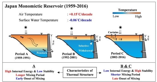
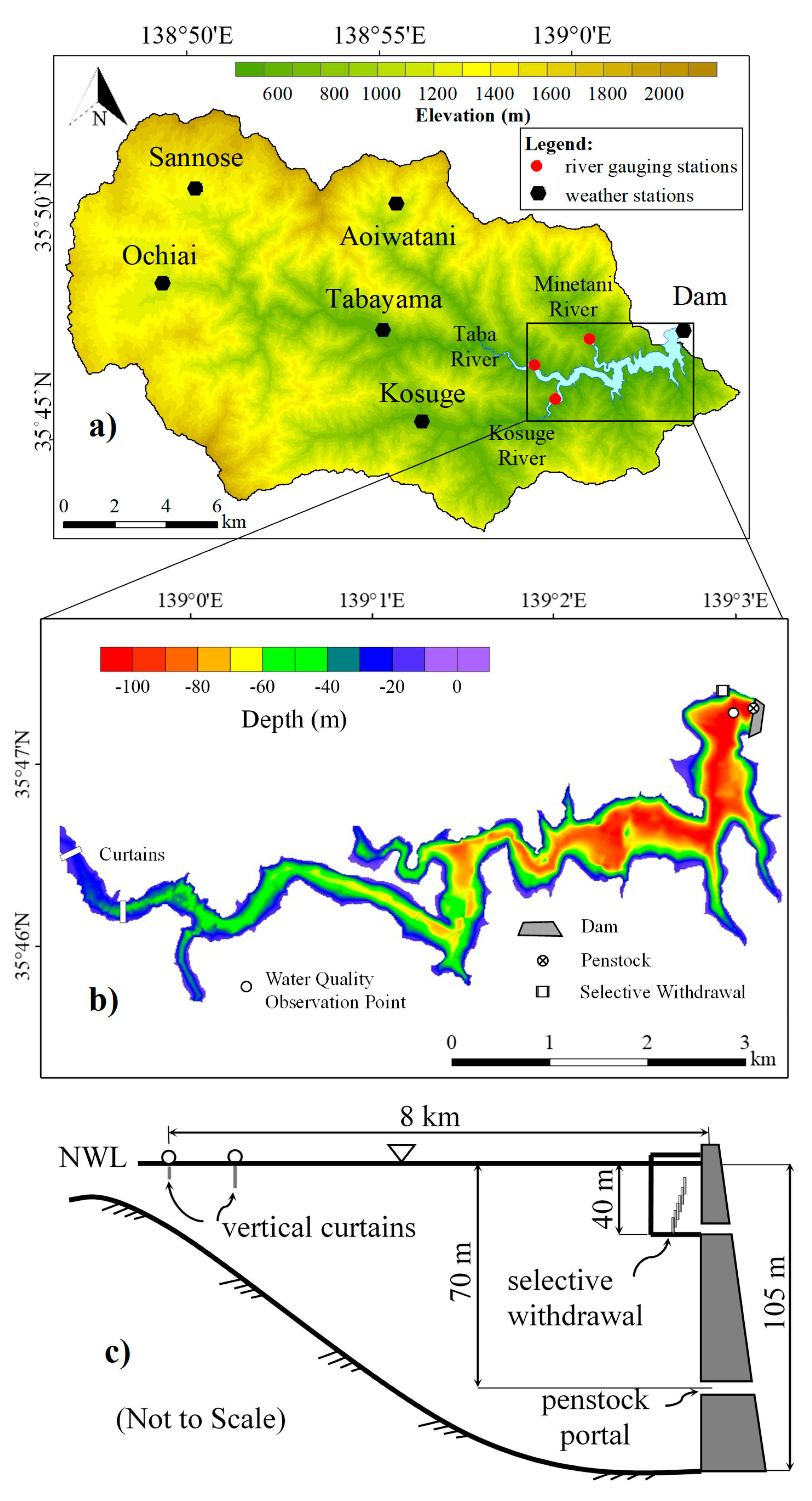
2.1. Site Background
2.2. Climate Analysis
2.3. Reservoir Temperatures
2.4. Thermal Structure Indicators
3. Results
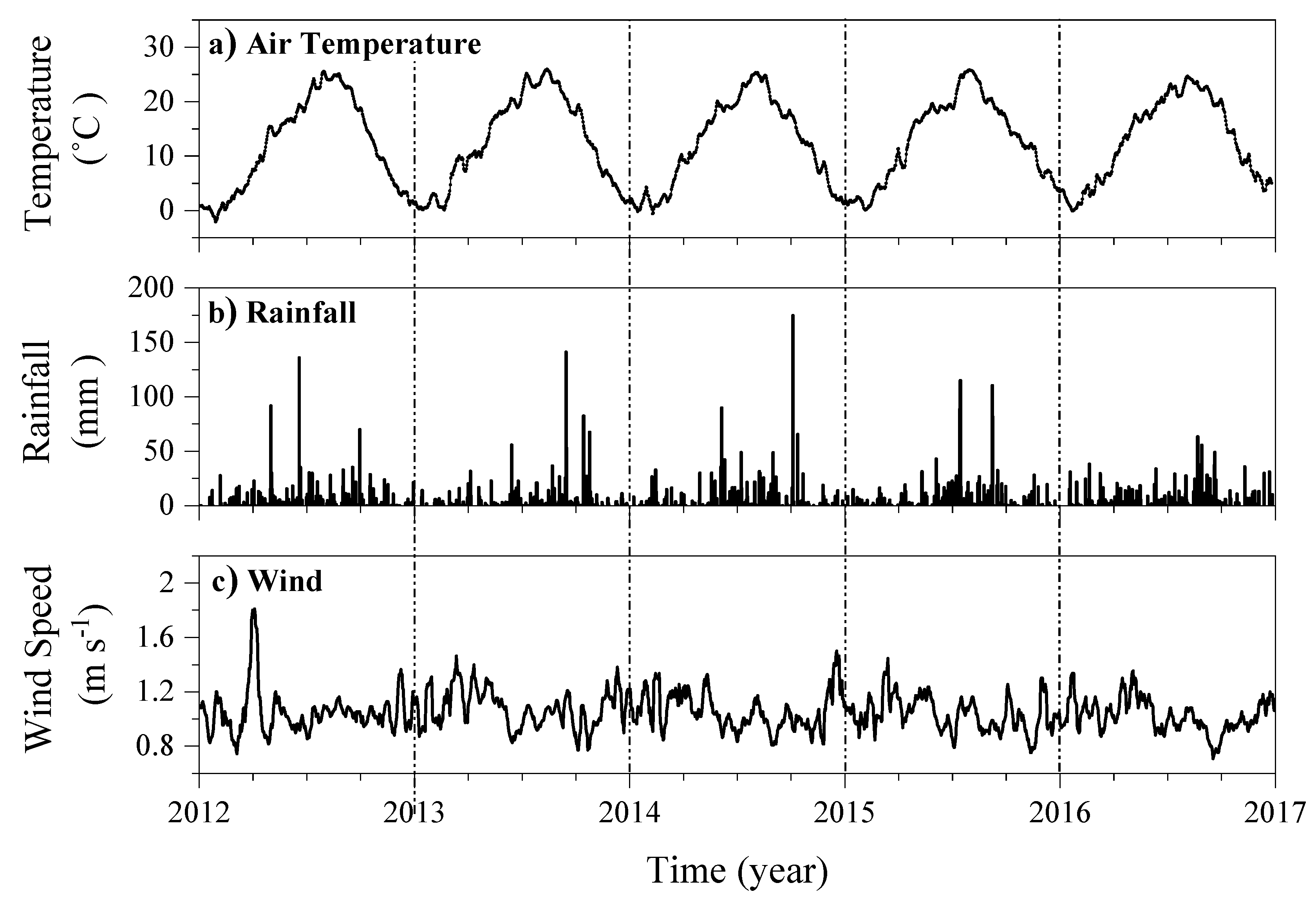
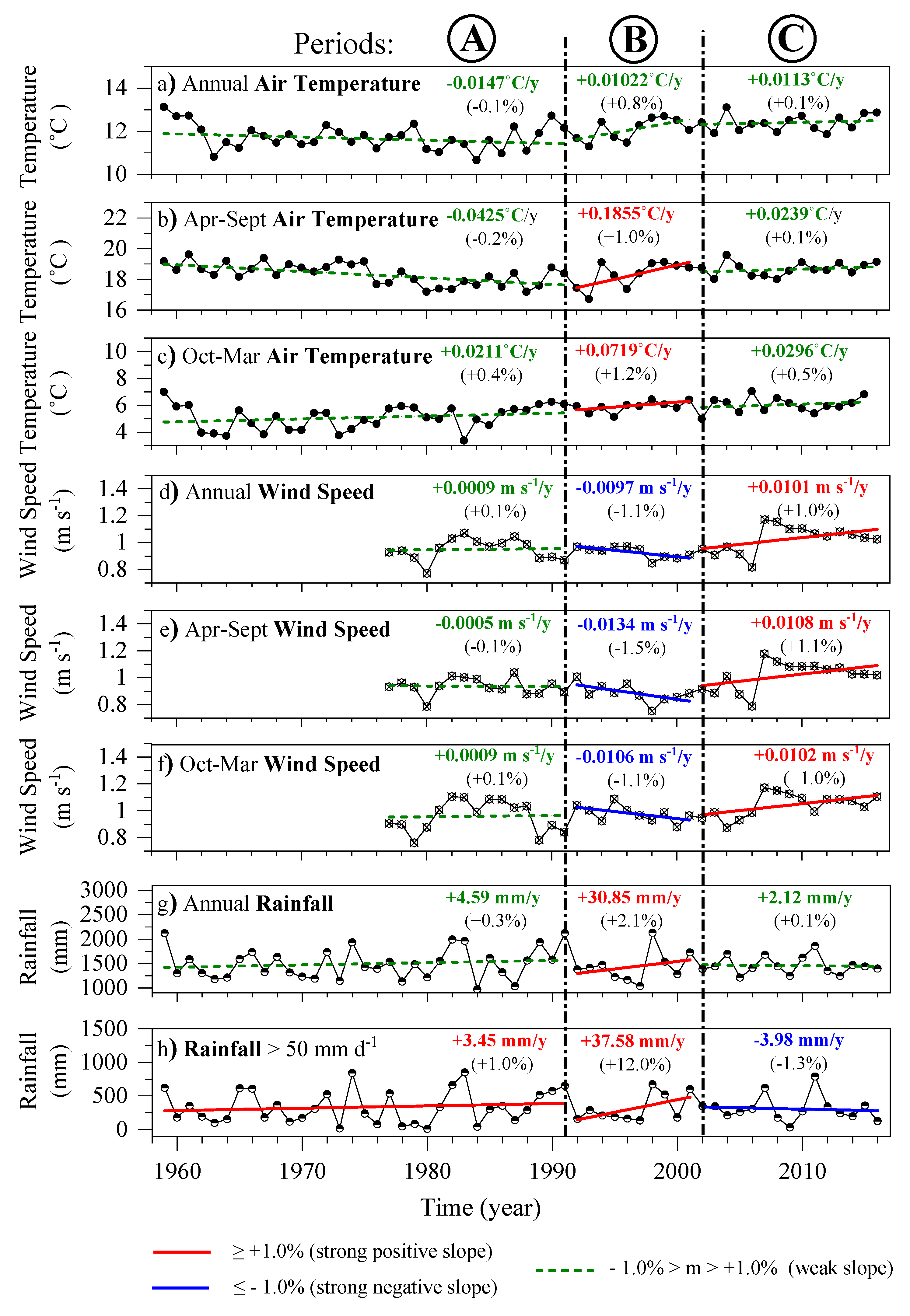
3.1. Climate Trends
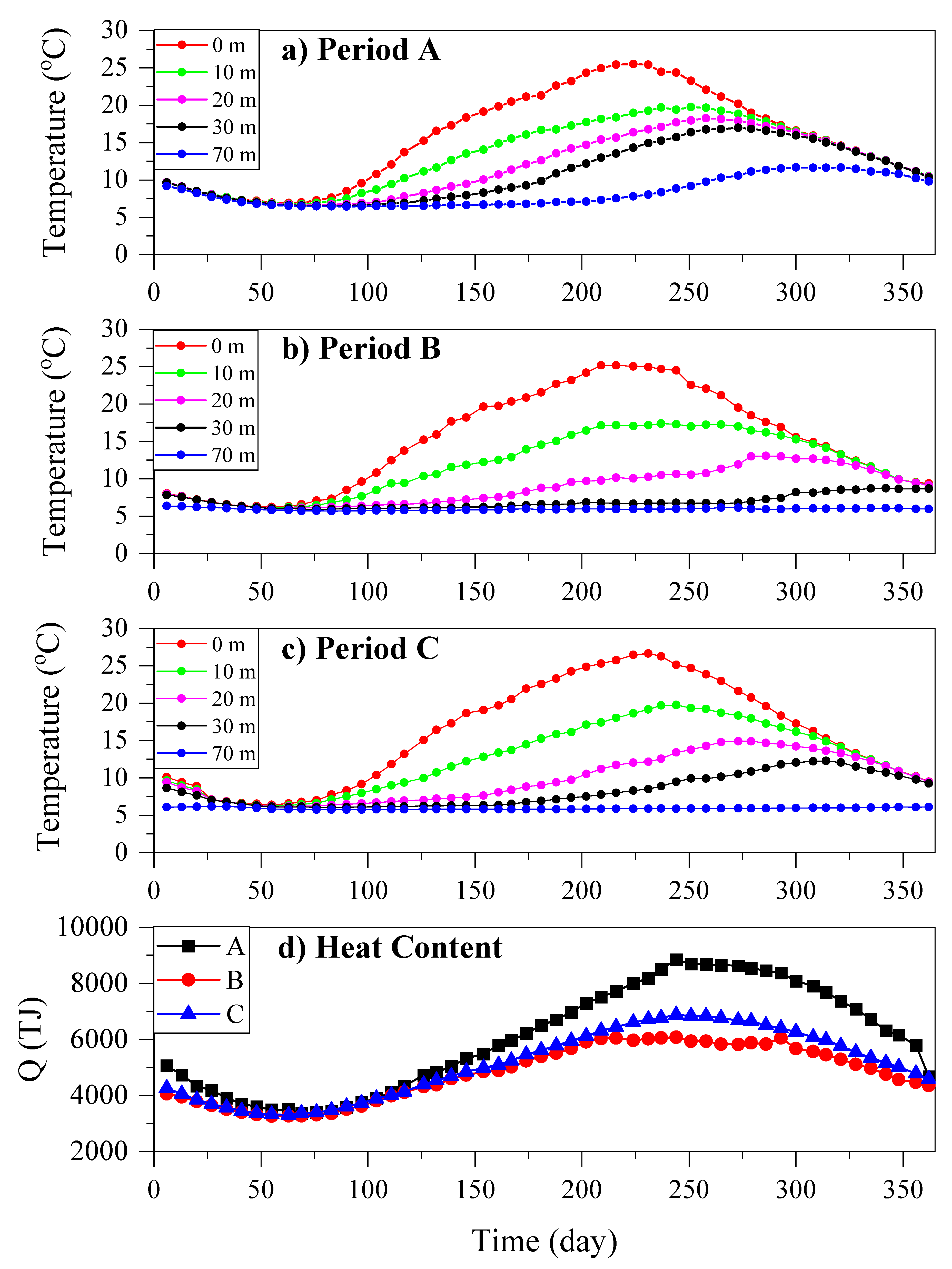
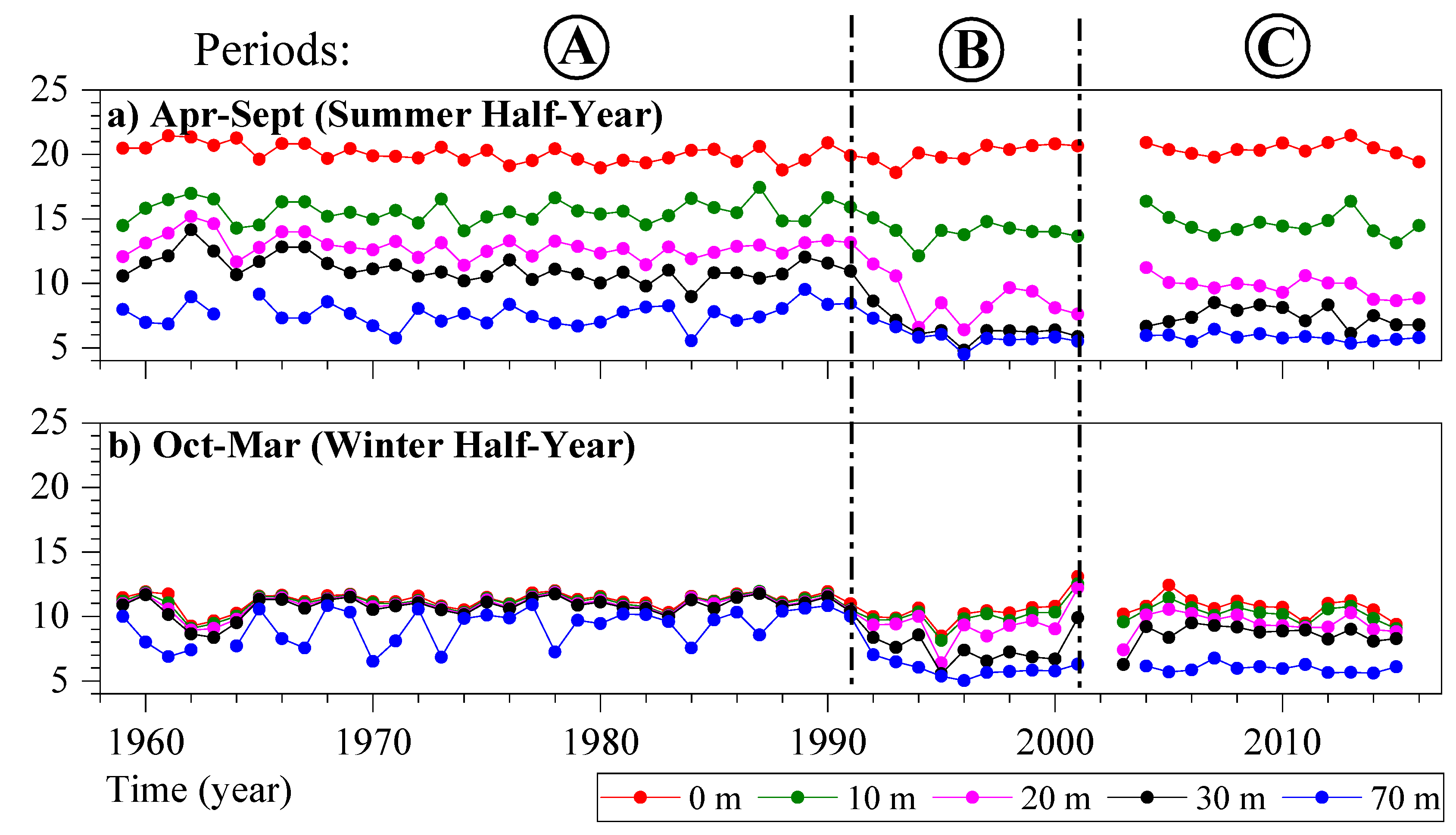
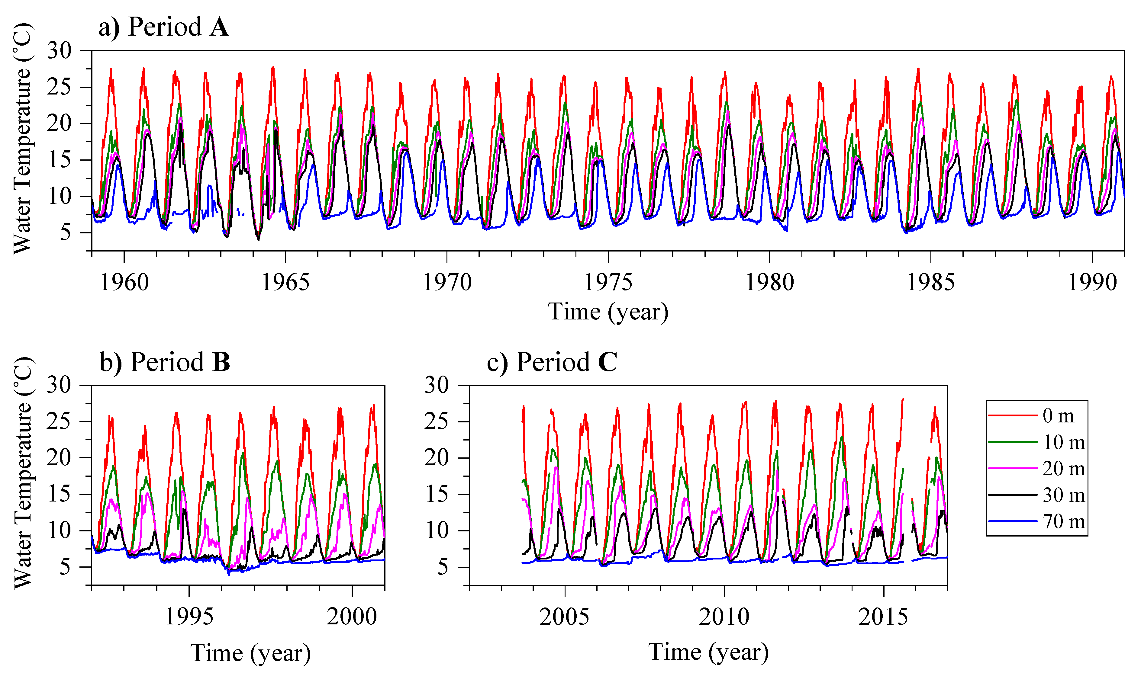
3.2. Water Temperature Distribution and Trends
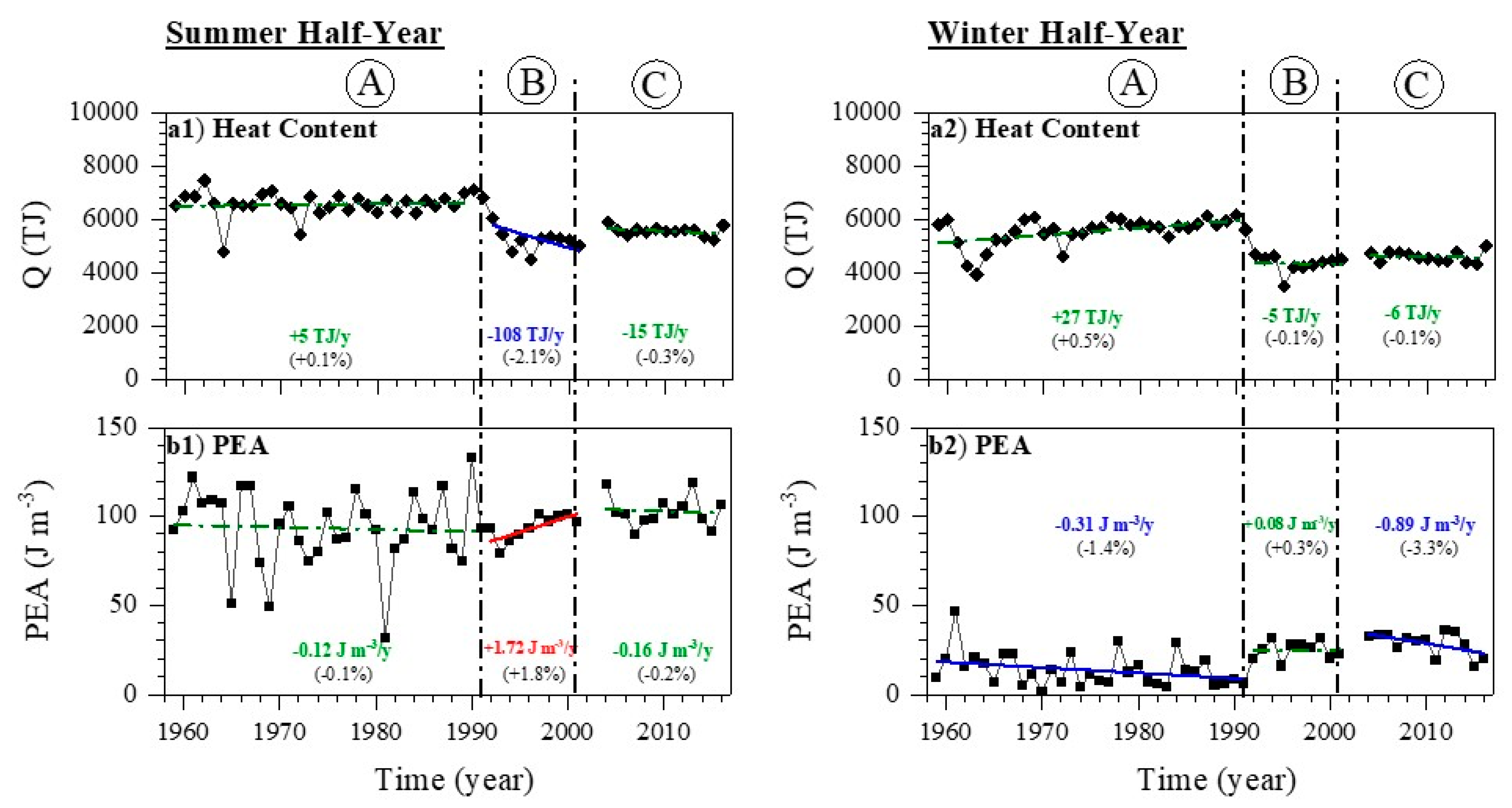
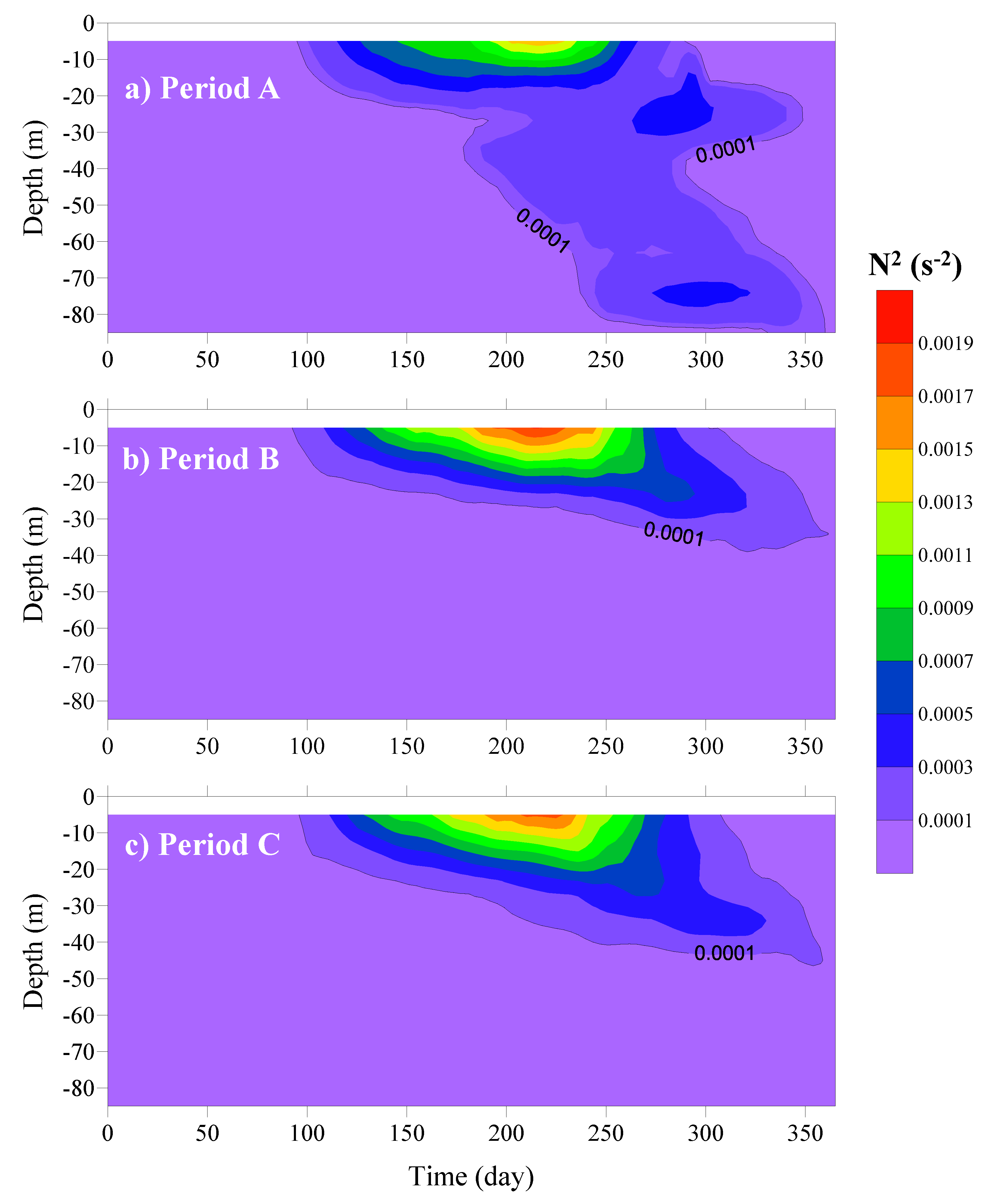
3.3. Thermal Structure Parameters
4. Discussion
4.1. Correlation Between Climate Forcing and Reservoir Temperatures
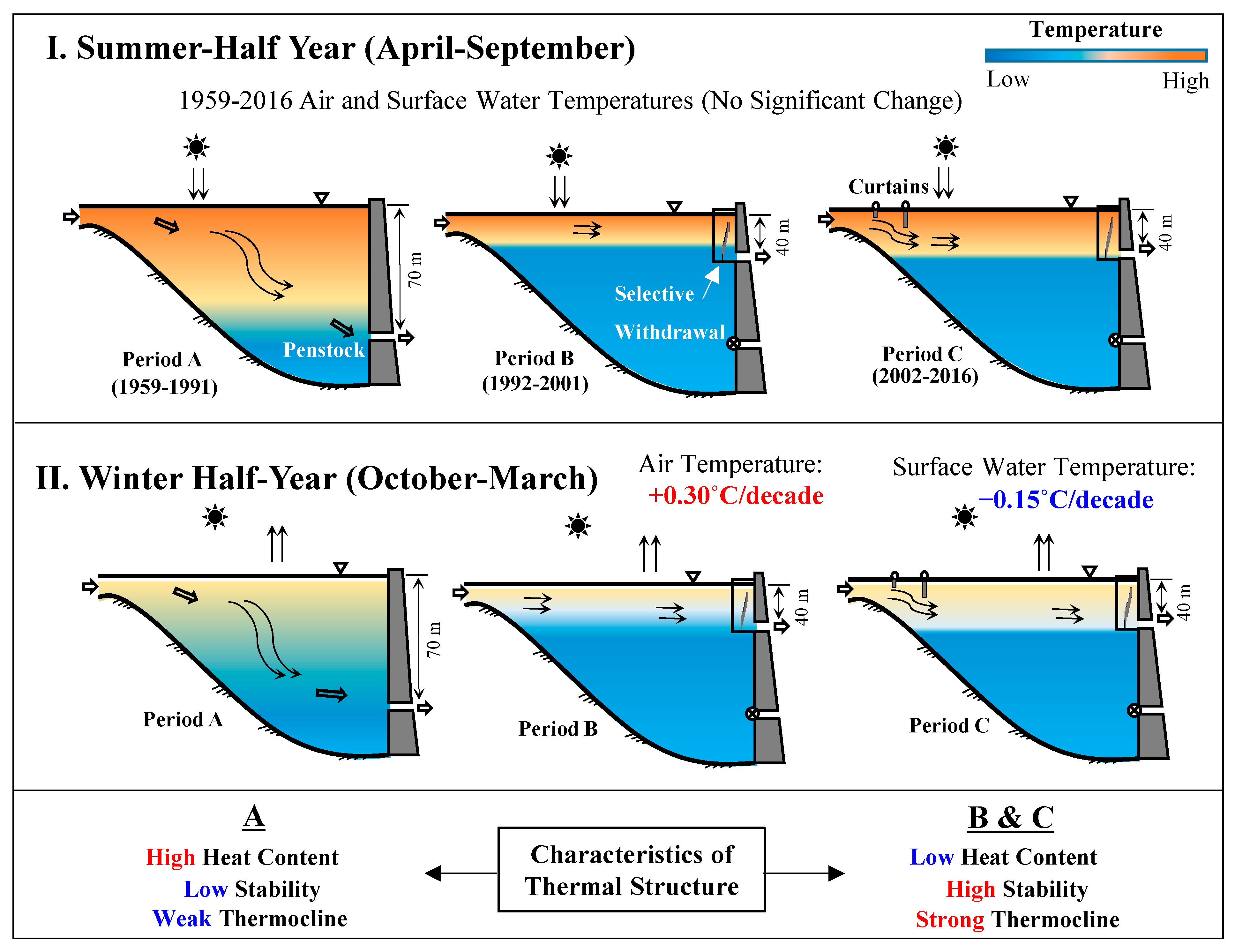
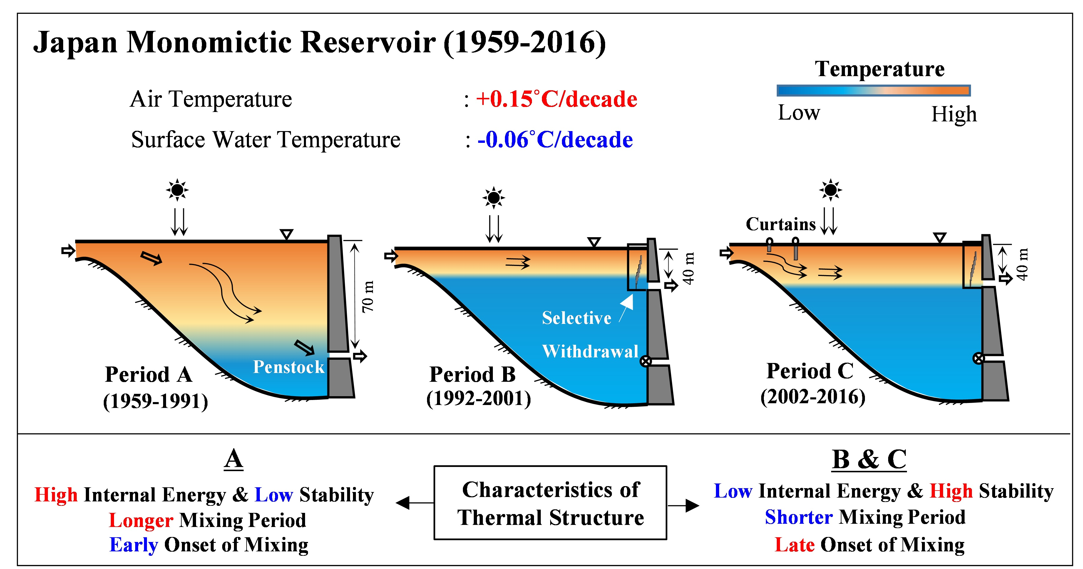
4.2. Effect of Facilities on Reservoir’s Thermal Structure
5. Conclusions
Author Contributions
Funding
Institutional Review Board Statement
Informed Consent Statement
Data Availability Statement
Acknowledgments
Conflicts of Interest
References
- Arvola, L.; George, G.; Livingstone, D.M.; Järvinen, M.; Blenckner, T.; Dokulil, M.T.; Jennings, E.; Aonghusa, C.N.; Nõges, P.; Nõges, T.; et al. The impact of the changing climate on the thermal characteristics of lakes. In The Impact of Climate Change on European Lakes; Springer: Dordrecht, The Netherlands; Heidelberg, Germany; London, UK; New York, NY, USA, 2009; pp. 85–101. [Google Scholar] [CrossRef]
- Coats, R.; Perez-Losada, J.; Schladow, G.; Richards, R.; Goldman, C. The warming of Lake Tahoe. Clim. Chang. 2006, 76, 121–148. [Google Scholar] [CrossRef]
- Rose, K.C.; Winslow, L.A.; Read, J.S.; Hansen, G.J.A. Climate-induced warming of lakes can be either amplified or suppressed by trends in water clarity. Limnol. Oceanogr. Lett. 2016, 1, 44–53. [Google Scholar] [CrossRef]
- Schmid, M.; Hunziker, S.; Wüest, A. Lake surface temperatures in a changing climate: A global sensitivity analysis. Clim. Chang. 2014, 124, 301–315. [Google Scholar] [CrossRef]
- Ficker, H.; Luger, M.; Gassner, H. From dimictic to monomictic: Empirical evidence of thermal regime transitions in three deep alpine lakes in Austria induced by climate change. Freshw. Biol. 2017, 62, 1335–1345. [Google Scholar] [CrossRef]
- Schneider, P.; Hook, S.J. Space observations of inland water bodies show rapid surface warming since 1985. Geophys. Res. Lett. 2010, 37, 1–5. [Google Scholar] [CrossRef] [Green Version]
- O’Reilly, C.M.; Sharma, S.; Gray, D.K.; Hampton, S.E.; Read, J.S.; Rowley, R.J.; Schneider, P.; Lenters, J.D.; McIntyre, P.B.; Kraemer, B.M.; et al. Rapid and highly variable warming of lake surface waters around the globe. Geophys. Res. Lett. 2015, 42, 10773–10781. [Google Scholar] [CrossRef] [Green Version]
- Woolway, R.I.; Weyhenmeyer, G.A.; Schmid, M.; Dokulil, M.T.; de Eyto, E.; Maberly, S.C.; May, L.; Merchant, C.J. Substantial increase in minimum lake surface temperatures under climate change. Clim. Chang. 2019, 155, 81–94. [Google Scholar] [CrossRef] [Green Version]
- Woolway, R.I.; Merchant, C.J. Worldwide alteration of lake mixing regimes in response to climate change. Nat. Geosci. 2019. [Google Scholar] [CrossRef]
- Helfer, F.; Lemckert, C.; Zhang, H. Impacts of climate change on temperature and evaporation from a large reservoir in Australia. J. Hydrol. 2012, 475, 365–378. [Google Scholar] [CrossRef] [Green Version]
- Trumpickas, J.; Shuter, B.J.; Minns, C.K. Forecasting impacts of climate change on Great Lakes surface water temperatures. J. Great Lakes Res. 2009, 35, 454–463. [Google Scholar] [CrossRef]
- Butcher, J.B.; Nover, D.; Johnson, T.E.; Clark, C.M. Sensitivity of lake thermal and mixing dynamics to climate change. Clim. Chang. 2015, 129, 295–305. [Google Scholar] [CrossRef] [Green Version]
- Adrian, R.; O’Reilly, C.M.; Zagarese, H.; Baines, S.B.; Hessen, D.O.; Keller, W.; Livingstone, D.M.; Sommaruga, R.; Straile, D.; Van Donk, E.; et al. Lakes as sentinels of climate change. Limnol. Oceanogr. 2009, 54, 2283–2297. [Google Scholar] [CrossRef] [PubMed]
- Lewis, W.M.; McCutchan, J.H.; Roberson, J. Effects of climatic change on temperature and thermal structure of a mountain reservoir. Water Resour. Res. 2019, 55, 1988–1999. [Google Scholar] [CrossRef]
- Zhang, Y.; Wu, Z.; Liu, M.; He, J.; Shi, K.; Zhou, Y.; Wang, M.; Liu, X. Dissolved oxygen stratification and response to thermal structure and long-term climate change in a large and deep subtropical reservoir (Lake Qiandaohu, China). Water Res. 2015, 75, 249–258. [Google Scholar] [CrossRef] [PubMed]
- Lee, R.M.; Biggs, T.W.; Fang, X. Thermal and hydrodynamic changes under a warmer climate in a variably stratified hypereutrophic reservoir. Water 2018, 10, 1284. [Google Scholar] [CrossRef] [Green Version]
- Azadi, F.; Ashofteh, P.S.; Loáiciga, H.A. Reservoir Water-Quality Projections under Climate-Change Conditions. Water Resour. Manag. 2019, 33, 401–421. [Google Scholar] [CrossRef]
- Chang, C.H.; Cai, L.Y.; Lin, T.F.; Chung, C.L.; Van Der Linden, L.; Burch, M. Assessment of the impacts of climate change on the water quality of a small deep reservoir in a humid-subtropical climatic region. Water 2015, 7, 1687–1711. [Google Scholar] [CrossRef] [Green Version]
- Martin, D.B.; Arneson, R.D. Comparative limnology of a deep-discharge reservoir and a surface-discharge lake on the Madison River, Montana. Freshw. Biol. 1978, 8, 33–42. [Google Scholar] [CrossRef]
- Hayes, N.M.; Deemer, B.R.; Corman, J.R.; Razavi, N.R.; Strock, K.E. Key differences between lakes and reservoirs modify climate signals: A case for a new conceptual model. Limnol. Oceanogr. Lett. 2017, 2, 47–62. [Google Scholar] [CrossRef]
- Moreno-Ostos, E.; Marcé, R.; Ordóñez, J.; Dolz, J.; Armengol, J. Hydraulic management drives heat budgets and temperature trends in a Mediterranean reservoir. Int. Rev. Hydrobiol. 2008, 93, 131–147. [Google Scholar] [CrossRef]
- Feldbauer, J.; Kneis, D.; Hegewald, T.; Berendonk, T.U.; Petzoldt, T. Managing climate change in drinking water reservoirs: Potentials and limitations of dynamic withdrawal strategies. Environ. Sci. Eur. 2020, 32, 1–17. [Google Scholar] [CrossRef] [Green Version]
- Duka, M.A.; Shintani, T.; Yokoyama, K. Thermal stratification responses of a monomictic reservoir under different seasons and operation schemes. Sci. Total Environ. 2020, 767, 1–15. [Google Scholar] [CrossRef]
- Olden, J.D.; Naiman, R.J. Incorporating thermal regimes into environmental flows assessments: Modifying dam operations to restore freshwater ecosystem integrity. Freshw. Biol. 2010, 55, 86–107. [Google Scholar] [CrossRef]
- Rheinheimer, D.E.; Null, S.E.; Lund, J.R. Optimizing Selective Withdrawal from Reservoirs to Manage Downstream Temperatures with Climate Warming. J. Water Resour. Plan. Manag. 2015, 141, 04014063. [Google Scholar] [CrossRef]
- Weber, M.; Rinke, K.; Hipsey, M.R.; Boehrer, B. Optimizing withdrawal from drinking water reservoirs to reduce downstream temperature pollution and reservoir hypoxia. J. Environ. Manag. 2017. [Google Scholar] [CrossRef] [PubMed]
- Çalişkan, A.; Elçi, Ş. Effects of selective withdrawal on hydrodynamics of a stratified reservoir. Water Resour. Manag. 2009, 23, 1257–1273. [Google Scholar] [CrossRef] [Green Version]
- Ma, S.; Kassinos, S.C.; Fatta Kassinos, D.; Akylas, E. Effects of selective water withdrawal schemes on thermal stratification in Kouris Dam in Cyprus. Lakes Reserv. Res. Manag. 2008, 13, 51–61. [Google Scholar] [CrossRef]
- Zouabi-Aloui, B.; Adelana, S.M.; Gueddari, M. Effects of selective withdrawal on hydrodynamics and water quality of a thermally stratified reservoir in the southern side of the Mediterranean Sea: A simulation approach. Environ. Monit. Assess. 2015, 187, 292. [Google Scholar] [CrossRef] [PubMed]
- Duka, M.A.; Yokoyama, K.; Shintani, T.; Iguchi, K.; Iwasaki, H.; Ueno, T.; Chiba, T. Influence of water control facilities on thermal stratification of Ogouchi Reservoir for 58 years. J. JSCE Ser. B1 2019, 75, 685–690. [Google Scholar] [CrossRef]
- Asaeda, T.; Pham, H.S.; Nimal Priyantha, D.G.; Manatunge, J.; Hocking, G.C. Control of algal blooms in reservoirs with a curtain: A numerical analysis. Ecol. Eng. 2001, 16, 395–404. [Google Scholar] [CrossRef]
- Park, C.H.; Park, M.H.; Kim, K.H.; Kim, N.Y.; Kim, Y.H.; Gwon, E.M.; Kim, B.H.; Lim, B.J.; Hwang, S.J. A physical pre-treatment method (VerticalWeir Curtain) for mitigating cyanobacteria and some of their metabolites in a drinking water reservoir. Water 2017, 9, 775. [Google Scholar] [CrossRef] [Green Version]
- Kumar Dutta, R.; Ma, J.; Das, B.; Liu, D. Modeling effects of floating curtain weirs and controlling algal Blooms in a subtropical reservoir of china. Am. J. Water Resour. 2019, 7, 42–49. [Google Scholar] [CrossRef]
- Johnson, P.; Vermeyen, T.; O’Haver, P. Use of flexible curtains to control reservoir release temperatures physical model and field prototype observations. In Proceedings of the 1993 USCOLD Annual Meeting, Chattanooga, TN, USA, May 1993; pp. 1–13. [Google Scholar]
- Johnson, P.; LaFond, R.; Webber, D.W. PAP-733 Temperature Control Device for Shasta Dam by Richard LaFond Presented to the Japan Dam Engineering Center November 1991; USBR: Washington, DC, USA, 1991.
- Deng, Y.; Tuo, Y.; Li, J.; Li, K.; Li, R. Spatial-temporal effects of temperature control device of stoplog intake for Jinping i hydropower station. Sci. China Technol. Sci. 2011, 54, 83–88. [Google Scholar] [CrossRef]
- Takahashi, T. The Influence of Surface Water Discharge on the Occurrence of Blue- Green Algae Water Bloom and Countermeasures to Prevent Blue- Green Algae Water Bloom from Occurring in the Ogochi Reservoir. In Proceedings of the IWA World Water Congress, Vienna, Austria, 7–12 September 2008. [Google Scholar]
- Niiyama, M.; Kouga, K.; Yokoyama, K.; Koizumi, A.; Yamazaki, K.; Masuko, A.; Kobayashi, Y.; Minegishi, N. Influence of the vertical fence on the movement of a density current in awater supply reservoir. J. JSCE Ser. B1 2010, 54, 1417–1422. [Google Scholar]
- Elçi, Ş. Effects of thermal stratification and mixing on reservoir water quality. Limnology 2008, 9, 135–142. [Google Scholar] [CrossRef] [Green Version]
- Noori, R.; Berndtsson, R.; Franklin Adamowski, J.; Rabiee Abyaneh, M. Temporal and depth variation of water quality due to thermal stratification in Karkheh Reservoir, Iran. J. Hydrol. Reg. Stud. 2018, 19, 279–286. [Google Scholar] [CrossRef]
- Japan Meteorological Agency. Overview of Japan’s Climate. n.d. Available online: https://www.data.jma.go.jp/gmd/cpd/longfcst/en/tourist_japan.html (accessed on 15 August 2019).
- Kendall, M.G. Rank Correlation Methods; Griffin: London, UK, 1975. [Google Scholar]
- Mann, H.B. Nonparametric Tests Against Trend. Econometrica 1945, 70, 245–259. [Google Scholar] [CrossRef]
- Sen, P.K. Estimates of the Regression Coefficient Based on Kendall’s Tau. J. Am. Stat. Assoc. 1968, 63, 1379–1389. [Google Scholar] [CrossRef]
- Pivato, M.; Carniello, L.; Viero DPietro Soranzo, C.; Defina, A.; Silvestri, S. Remote sensing for optimal estimation of water temperature dynamics in shallow tidal environments. Remote Sens. 2020, 12, 51. [Google Scholar] [CrossRef] [Green Version]
- Simpson, J.H. The shelf-sea fronts: Implications of their existence and behaviour. Philos. Trans. R. Soc. London. Ser. A Math. Phys. Sci. 1981, 302, 531–546. [Google Scholar] [CrossRef]
- Yamaguchi, R.; Suga, T.; Richards, K.J.; Qiu, B. Diagnosing the development of seasonal stratification using the potential energy anomaly in the North Pacific. Clim. Dyn. 2019, 53, 4667–4681. [Google Scholar] [CrossRef]
- Durran, D.R.; Klemp, J.B. On the effects of moisture on the Brunt-Vaisala frequency. J. Atmos. Sci. 1982, 39, 2152–2158. [Google Scholar] [CrossRef]
- Japan Meteorological Agency. Climate Change Monitoring Report 2016; JMA: Chiyoda, Tokyo, 2017.
- Matsumoto, J.; Fujibe, F.; Takahashi, H. Urban climate in the Tokyo metropolitan area in Japan. J. Environ. Sci. 2017, 59, 54–62. [Google Scholar] [CrossRef] [PubMed]
- Xu, Z.; Takeuchi, K.; Ishidaira, H. Long-term trends of annual temperature and precipitation time series in Japan. J. Hydrosci. Hydraul. Eng. 2002, 20, 11–26. [Google Scholar]
- Mi, C.; Sadeghian, A.; Lindenschmidt, K.E.; Rinke, K. Variable withdrawal elevations as a management tool to counter the effects of climate warming in Germany’s largest drinking water reservoir. Environ. Sci. Eur. 2019, 31, 1–15. [Google Scholar] [CrossRef] [Green Version]


| Parameters | Station | Elevation (above msl) | Period Covered | Frequency |
|---|---|---|---|---|
| Air temperature (°C) | Dam | 519 m | 1959–2016 | Daily |
| Precipitation (mm) | (1) Dam (2) Ochiai (3) Tabayama (4) Kosuge (5) Aoiwatani (6) Sannose | 519 m 1113 m 611 m 656 m 1217 m 1268 m | 1959–2016 1959–2016 1959–2016 1959–2016 1965–2016 1965–2016 | Daily Daily Daily Daily Daily Daily |
| Wind Speed (m s−1) | Dam | 519 m | 1977–2016 | Daily |
| Water temperature profile (°C) | Upstream of Dam Wall | 1959–2001 2003–2016 | Weekly Daily |
| Parameter | Period | M–K z-Stat | M–K p-Value | Sen’s Slope |
|---|---|---|---|---|
| Air Temperature | Annual | +2.9783 | 0.0029 | +0.15 °C decade−1 |
| Apr–Sept | −0.1610 | 0.8271 | −0.01 °C decade−1 | |
| Oct–Mar | +4.4809 | <0.0001 | +0.30 °C decade−1 | |
| Wind Speed | Annual | +1.8758 | 0.0607 | +0.03 m s−1 decade−1 |
| Apr–Sept | +1.4565 | 0.1453 | +0.02 m s−1 decade−1 | |
| Oct–Mar | +1.8293 | 0.0673 | +0.03 m s−1 decade−1 | |
| Rainfall | Annual | +0.2147 | 0.8300 | +5.02 mm decade−1 |
| >50 mm d−1 | +0.2415 | 0.8092 | +3.35 mm decade−1 | |
| SWT | Annual | −1.2723 | 0.2033 | −0.06 °C decade−1 |
| Apr–Sept | +0.0566 | 0.9549 | <0.01 °C decade−1 | |
| Oct–Mar | −2.3253 | 0.0201 | −0.15 °C decade−1 |
| Depth | Season | Average per Period (°C) | K–W p-Value | ||
|---|---|---|---|---|---|
| A | B | C | |||
| 0 m | Apr–Sept | 20.09 | 20.09 | 20.40 | 3.6 × 10⁻¹ |
| Oct–Mar | 11.23 | 10.44 * | 10.73 * | 1.9 × 10⁻³ | |
| 10 m | Apr–Sept | 15.58 | 13.98 * | 14.61 * | 8.4 × 10⁻⁶ |
| Oct–Mar | 11.06 | 10.08 * | 10.22 * | 1.6 × 10⁻³ | |
| 20 m | Apr–Sept | 12.87 | 8.63 * | 9.75 * | 1.9 × 10⁻⁹ |
| Oct–Mar | 10.91 | 9.31 * | 9.47 * | 4.7 × 10⁻⁶ | |
| 30 m | Apr–Sept | 11.14 | 6.40 * | 7.41 * | 1.2 × 10⁻⁹ |
| Oct–Mar | 10.76 | 7.46 * | 8.61 * | 1.0 × 10⁻⁸ | |
| 70 m | Apr–Sept | 7.59 | 5.85 * | 5.79 * | 1.4 × 10⁻⁷ |
| Oct–Mar | 9.20 | 5.91 * | 5.97 * | 7.0 × 10⁻⁹ | |
Publisher’s Note: MDPI stays neutral with regard to jurisdictional claims in published maps and institutional affiliations. |
© 2021 by the authors. Licensee MDPI, Basel, Switzerland. This article is an open access article distributed under the terms and conditions of the Creative Commons Attribution (CC BY) license (https://creativecommons.org/licenses/by/4.0/).
Share and Cite
Duka, M.A.; Shintani, T.; Yokoyama, K. Mediating the Effects of Climate on the Temperature and Thermal Structure of a Monomictic Reservoir through Use of Hydraulic Facilities. Water 2021, 13, 1128. https://doi.org/10.3390/w13081128
Duka MA, Shintani T, Yokoyama K. Mediating the Effects of Climate on the Temperature and Thermal Structure of a Monomictic Reservoir through Use of Hydraulic Facilities. Water. 2021; 13(8):1128. https://doi.org/10.3390/w13081128
Chicago/Turabian StyleDuka, Maurice Alfonso, Tetsuya Shintani, and Katsuhide Yokoyama. 2021. "Mediating the Effects of Climate on the Temperature and Thermal Structure of a Monomictic Reservoir through Use of Hydraulic Facilities" Water 13, no. 8: 1128. https://doi.org/10.3390/w13081128