
On Ripples—A Boundary Layer-Theoretical Definition


Abstract
1. Introduction
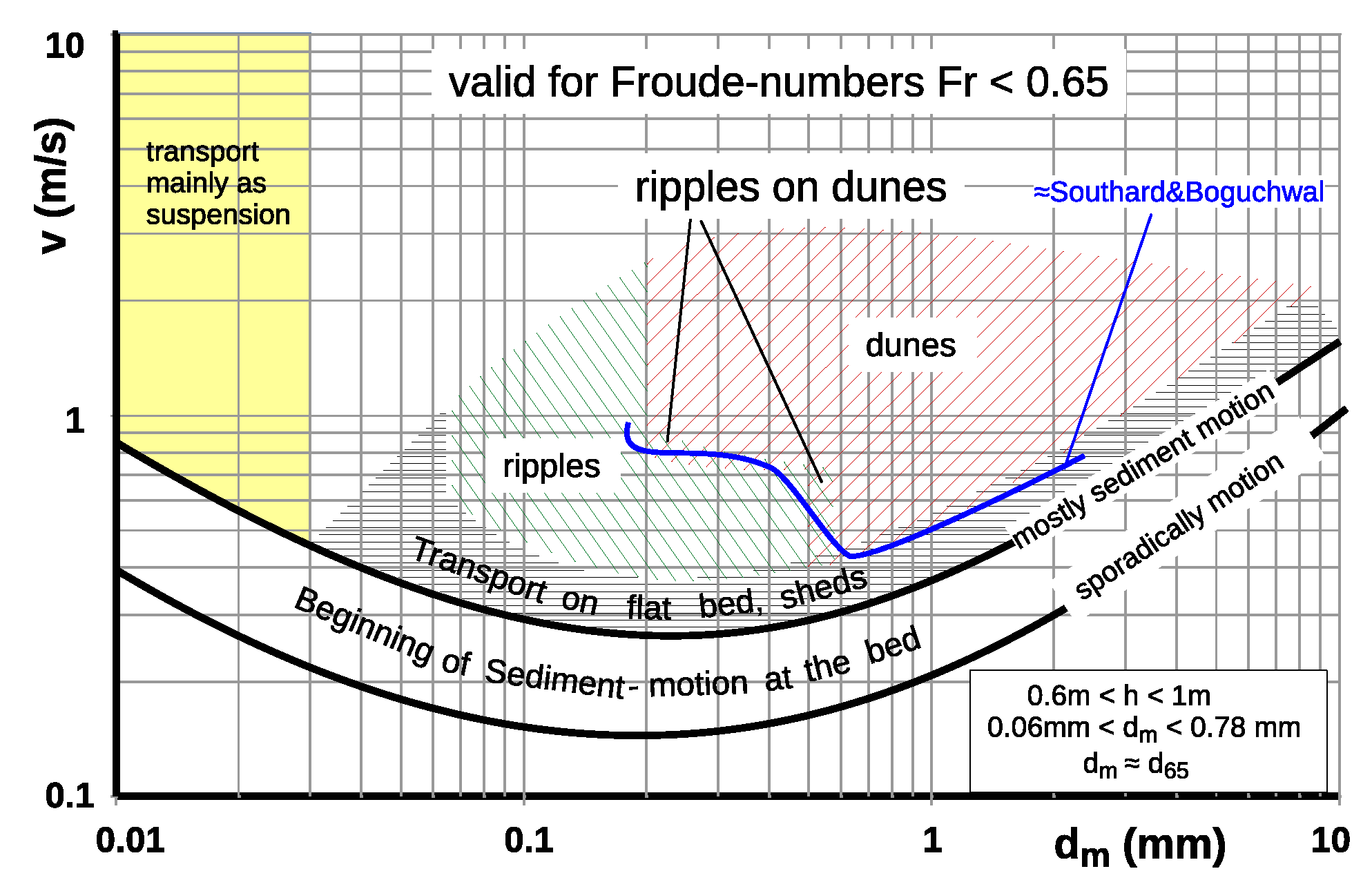
2. A Brief Description of the State of Research on the Distinction of Ripples and Dunes
3. Data Used for Comparison Purposes
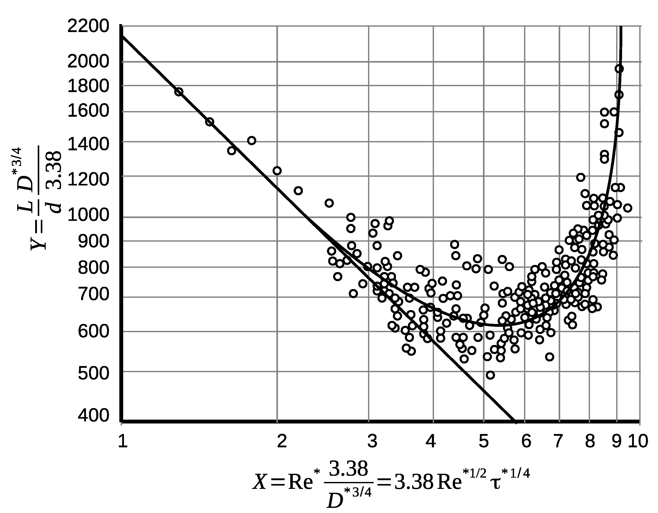
4. Semi Analytical Approach to Length and Domain of Ripples
4.1. Theory
4.2. Consideration of the Effect of Sediment Suspension
4.3. Consideration of the Effect of Acceleration of the Boundary Layer Flow
4.3.1. Acceleration-Related Maintenance of Viscous Boundary Layer
4.3.2. Solution Proposal for the Calculation of the Effect of Boundary Layer Acceleration
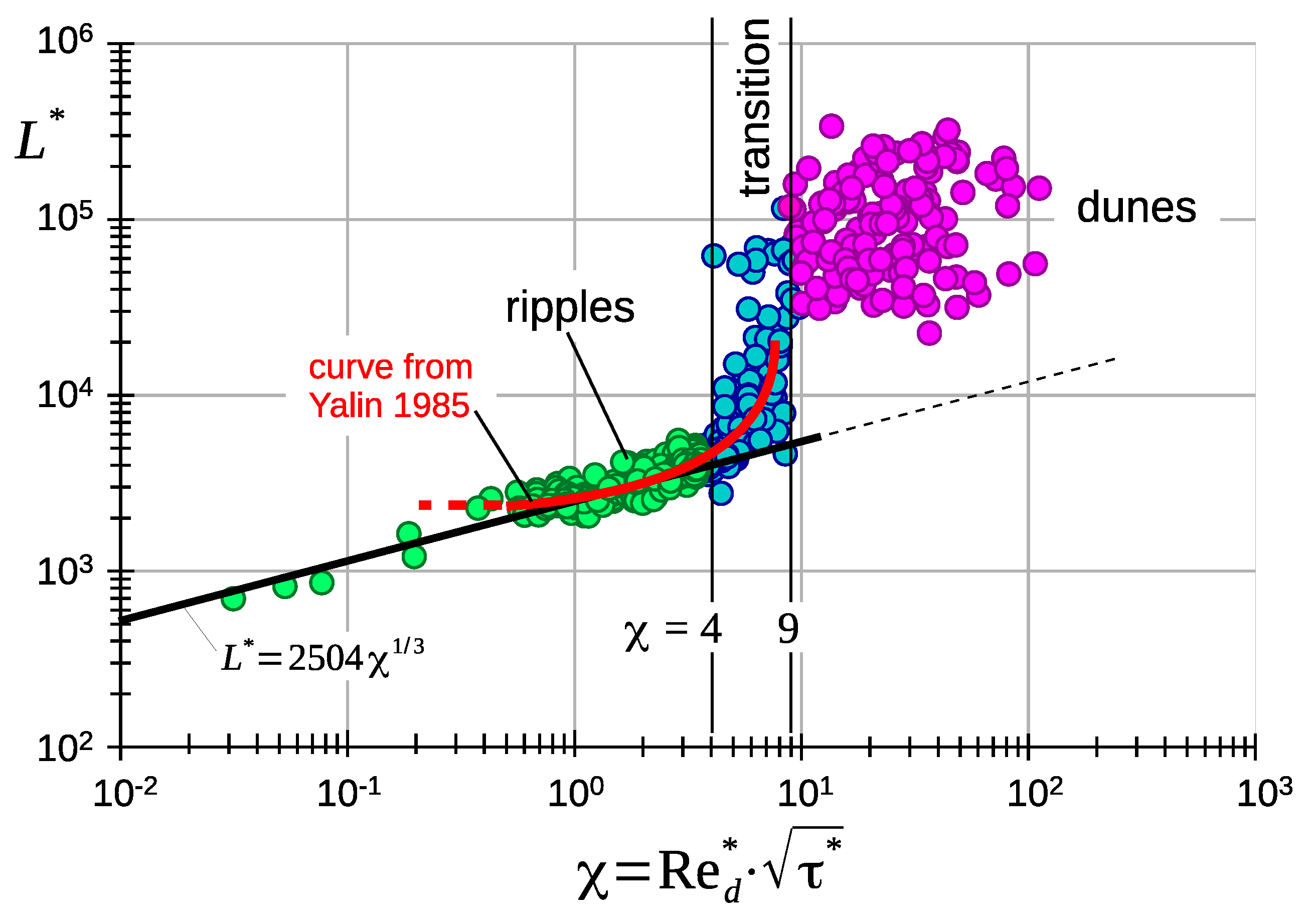
5. Reflections on the Limits of the Ripple Domain
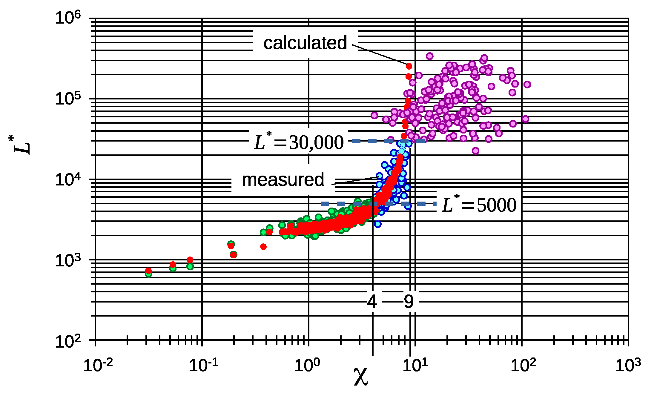
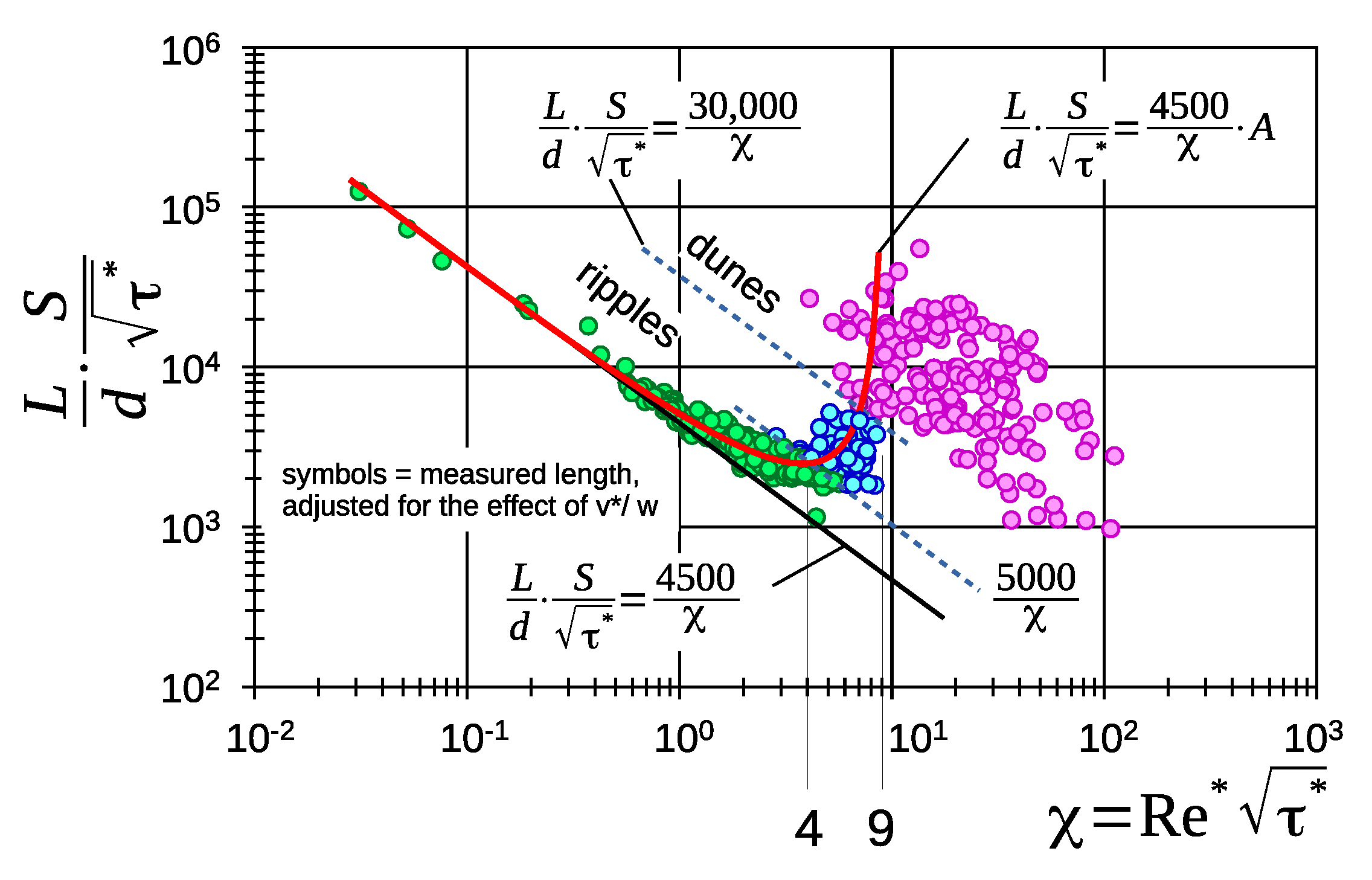
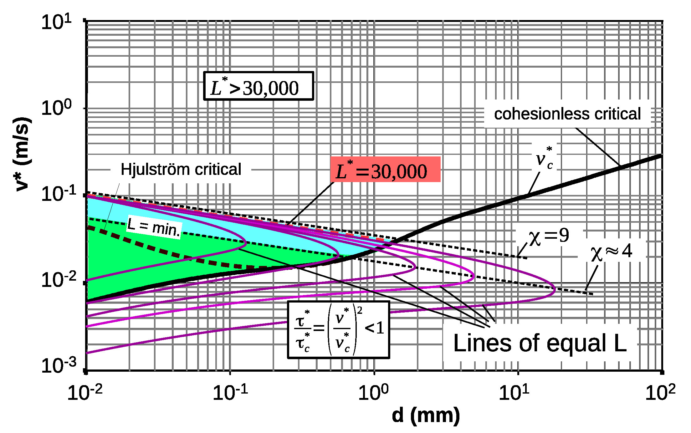
5.1. Upper Limit
5.2. On the Lower Limit Particle Size of Ripple Existence
5.3. The Transition Range
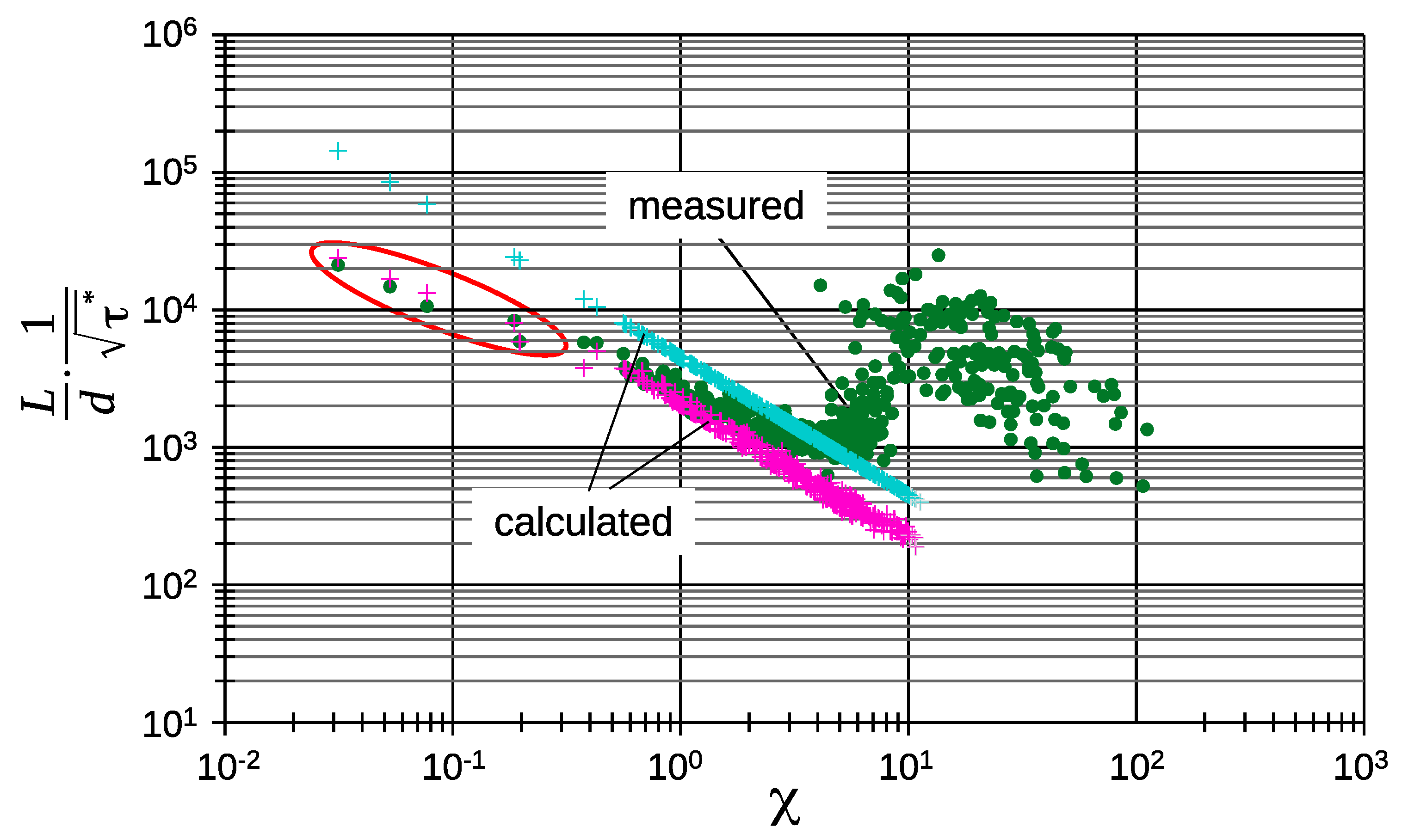
6. An Alternative Presentation of Data Only by Boundary Layer Effects
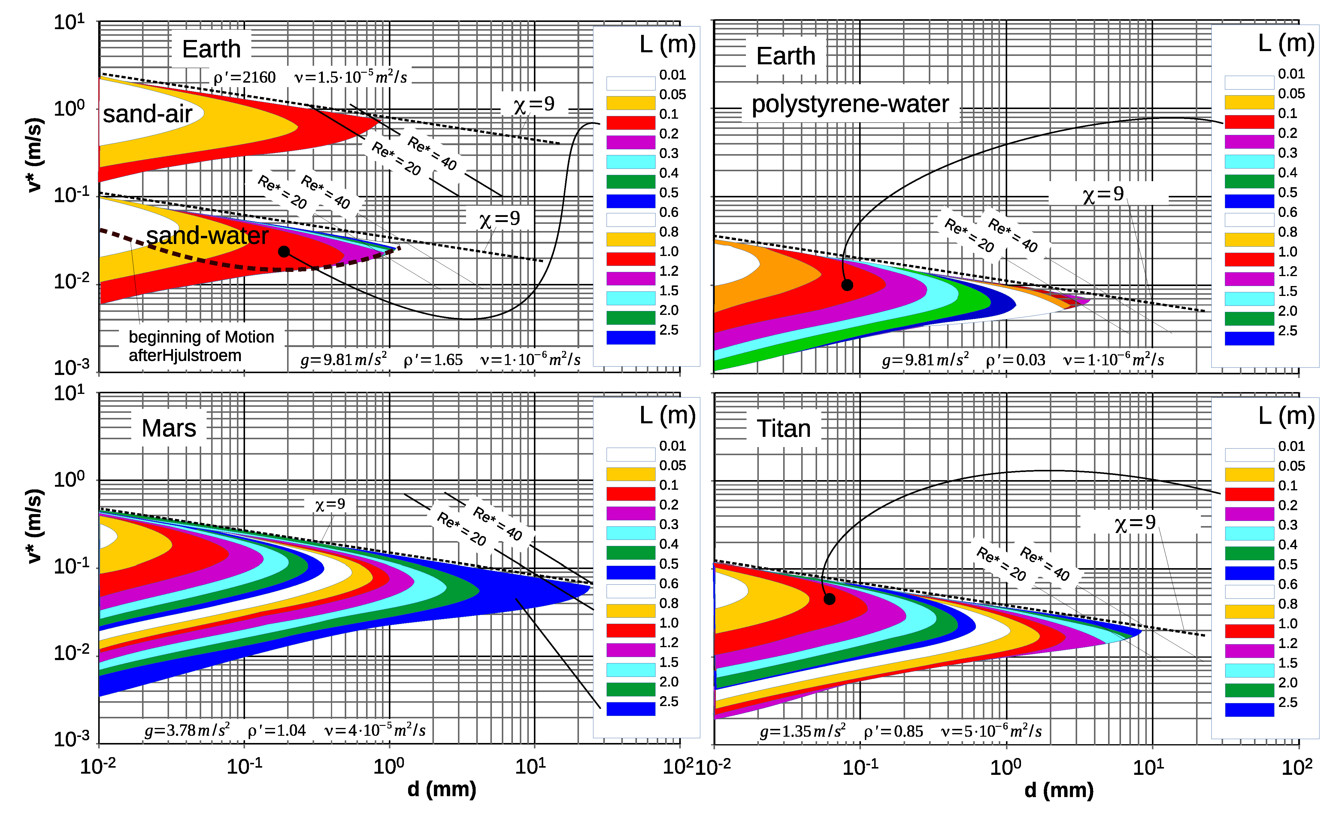
7. Examples of Ripple Domain and Length on Earth, Mars, and Titan
- (1)
- Critical shear stress. Ripples only develop when and 30,000 which coincides with .
- (2)
8. Discussion
9. Conclusions
Author Contributions
Funding
Institutional Review Board Statement
Informed Consent Statement
Data Availability Statement
Conflicts of Interest
Symbols
| Factor of flow acceleration effect on viscous boundary layer, Equation (33) | - | |
| critical Reynolds number für turn from laminar to turbulent boundary layer | - | |
| same as but in case of accelerated flow | - | |
| local drag coefficient | - | |
| d | grain diameter | m |
| mean grain diameter | m | |
| Grain size, which is exceeded by of its weight | m | |
| dimensionless grain diameter = | - | |
| g | acceleration of gravity | m/s2 |
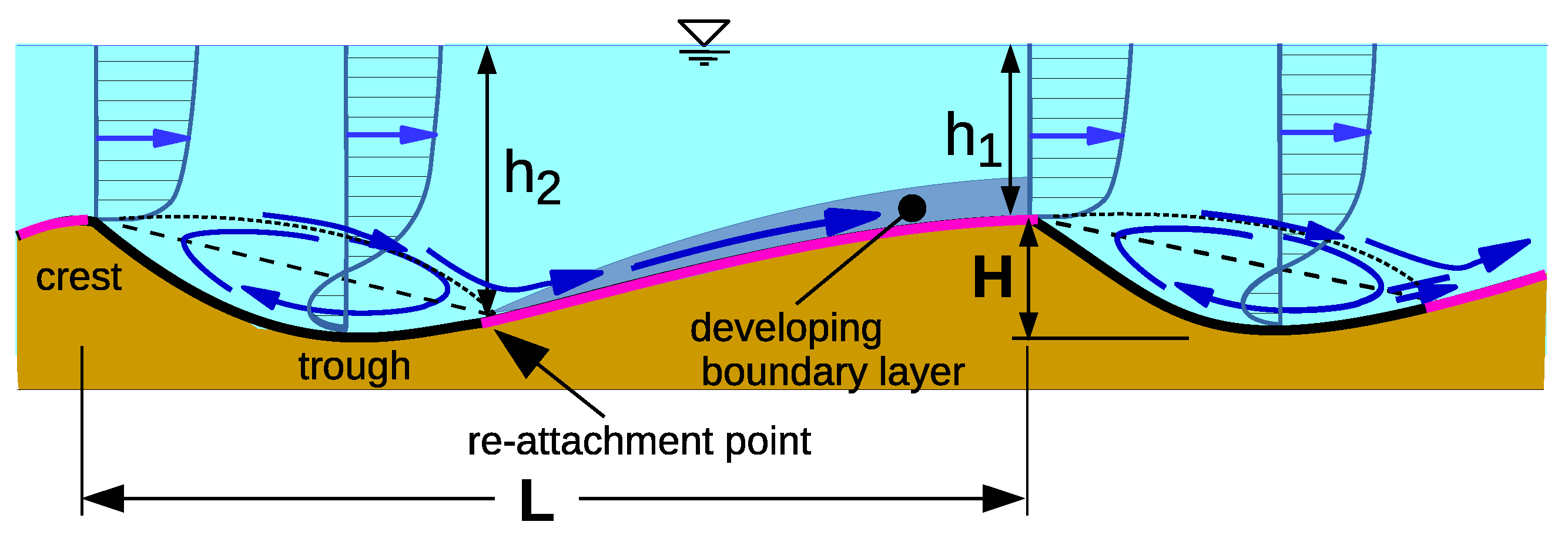
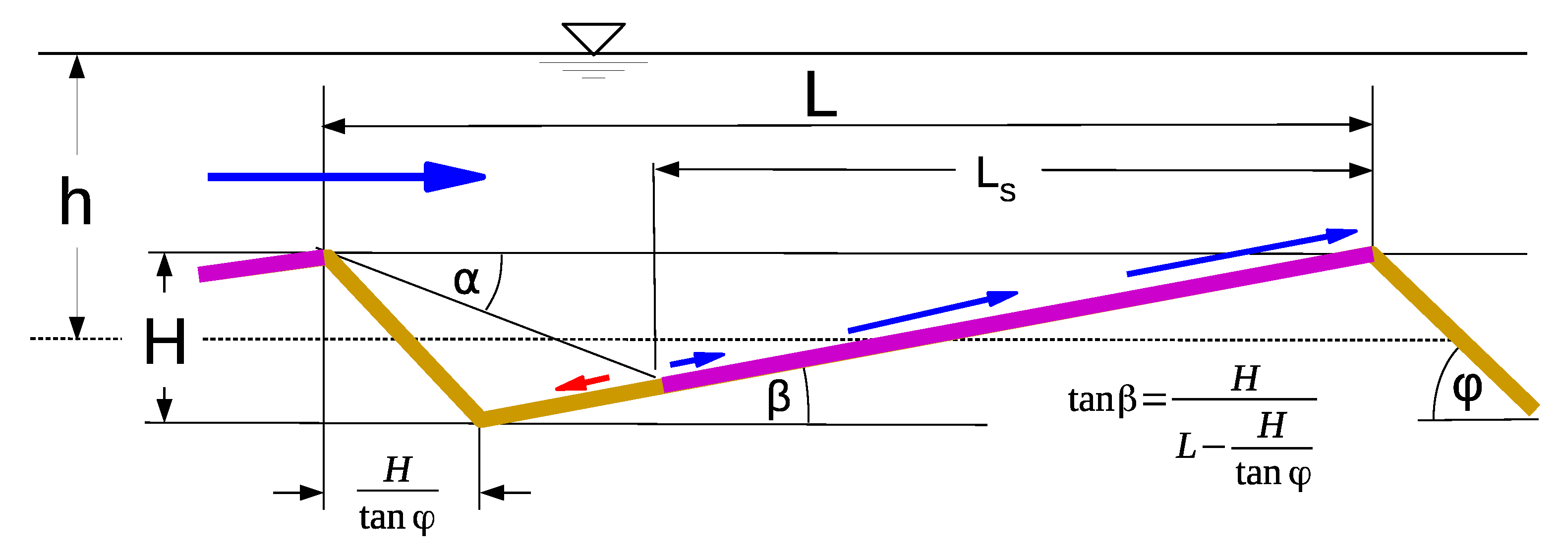
| H | height of bed forms | m |
| h | mean water depth = (Figure 2) | m |
| water depth over the crests of ripples and dunes | m | |
| K | key parameter describing the ability to relaminarize a viscous boundary layer, Equation (25) | - |
| L | length of bed forms | m |
| = | - | |
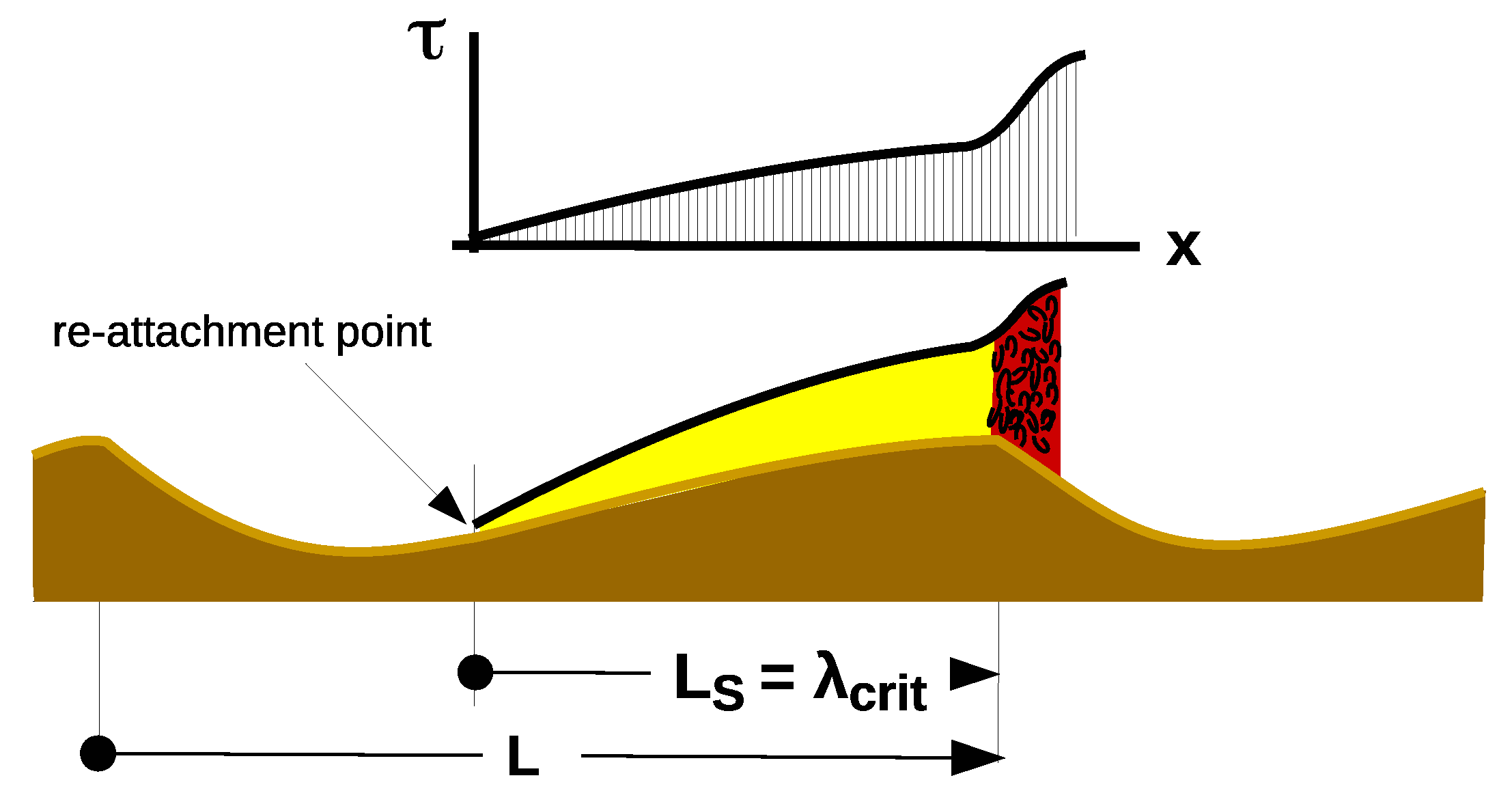
| partial length of bed forms with significant skin friction | m | |
| = , particle Reynolds number | - | |
| S | factor describing the effect of suspension on ripple length, Equation (20) | - |
| depth and time averaged flow velocity | m/s | |
| velocity of the outer flow of the boundary layer | m/s | |
| shear velocity = | m/s | |
| w | settling velocity | m/s |
| angle of free turbulence | ||
| angle of inclination of the windward slope of ripple and dunes | ||
| critical length after which the boundary layer switches from viscous to turbulent | m | |
| kinematic viscosity of fluid | m2/s | |
| density of fluid | kg/m3 | |
| density of sediment | kg/m3 | |
| , relative density | - | |
| , shear stress at the bed | N/m2 | |
| , dimensionless shear stress | - | |
| angle of repose = angle of internal friction of sediment | ||
| Yalin number as defined by Lapotre et al. [17], Equation (5) | - |
References
- Plate, E.J. Ein Beitrag zur Bestimmung der Windgeschwindigkeitsverteilung in Einer Durch Eine Wand Gestörten Bodennahen Luftschicht [A Contribution to the Determination of the Wind Speed Distribution in a Near-Bed Air Layer Disturbed by a Wall]; Diss. Techn. Hochschule (TH): Stuttgart, Germany, 1966. (In German) [Google Scholar]
- Yalin, M.S. Geometrical Properties of Sand-Waves. Proc. ASCE 1964, 90, HY5. [Google Scholar]
- Allen, J.R.L. Current Ripples; North Holland Publishing Company: Amsterdam, The Netherlands, 1968. [Google Scholar]
- Kennedy, J.F. The Formation of Sediment Ripples, Dunes and Antidunes. Annu. Rev. Fluid Mech. 1969, 1, 147–168. [Google Scholar] [CrossRef]
- Fredsoe, J. Sediment Ripples and Dunes. Ann. Rev. Fluid Mech. 1982, 14, 13–37. [Google Scholar]
- Ashley, G.M. Classification of large-scale subaquaeous bed forms: A new look on an old problem. J. Sediment. Petrol. 1990, 60, 160–172. [Google Scholar]
- Zanke, U. Über den Einfluß von Kornmaterial, Strömungen und Wasserständen auf die Transportkörper in Offenen Gerinnen [On the Effect of Bedmaterial, Currents and Water Depth on the Parameters of Ripples and Dunes in Open Channels]; Mitt. des Franzius-Instituts der TU Hannover: Hannoverm, Germany, 1976; Volume 44. (In German) [Google Scholar]
- Southard, J.; Boguchwal, A. Bed configurations in steady unidirectional water flows. Synthesis of flume data. J. Sediment. Petrol. 1990, 60 Pt 2, 658–679. [Google Scholar] [CrossRef]
- Chabert, J.; Chauvin, J.L. Formation des dunes et des rides dans les modèles fluviaux. Bull. CREC Chatou 1963, 4, 1–51. [Google Scholar]
- Bonnefille, R.; Pernecker, L. Le début d’entraînement des sediments sous l’action de la ‘houle. Bull. CREC Chatou 1966, 15. [Google Scholar]
- Vollmers, H.; Giese, E. Discussion on “Instability of Flat Bed in Alluvial Channels”. Proc. ASCE 1970. [Google Scholar] [CrossRef]
- Wieprecht, S. Entstehung und Verhalten von Transportkörpern bei Grobem Sohlenmaterial [Origin and Behavior of Dunes in Coarse Bed Material]; University of the German Federal Armed Forces: Neubiberg, Germany, 2001; ISBN 3-486-26518-0. (In German) [Google Scholar]
- Van den Berg, J.H.; van Gelder, A. A new bedform stability diagram, with emphasis on the transition of ripples to lane flows over fine sand. Spec. Publ. Int. Ass. Sediment 1993, 17, 11–21. [Google Scholar]
- Burr, M.; Perron, J.T.; Lamb, M.P.; Rossman, P.I.; Collins, G.C.; Howard, L.S.; Moore, J.M.; Adamkovics, M.; Baker, V.R.; Drummond, S.A.; et al. Fluvial features on Titan: Insight from morphology and modeling. Geol. Soc. Am. Bull. 2013, 125, 299–321. [Google Scholar] [CrossRef]
- Kleinhans, M.G. Phase Diagrams of Bed States in Steady, Unsteady, Oscillatory and Mixed Flows; Geology Utrecht University: Utrecht, The Netherlands, 2005; Corpus ID: 56390344. [Google Scholar]
- Yalin, M.S. On the Determination of Ripple Geometry. ASCE J. Hydraul. Eng. 1985, 111, 1148–1155. [Google Scholar] [CrossRef]
- Lapotre, M.G.A.; Lamb, M.P.; McElroy, B. What Sets the Size of Current Ripples? The Geological Society of America: Boulder, CO, USA, 2017. [Google Scholar]
- Barton, J.R.; Lin, P. A Study of the Sediment Transport an Alluvial Channels; Report No. 55, JRB 2; Civil Engineering Department, Colorado A and M College, Agricultural and Mechanical College: Fort Collins, CO, USA, 1955. [Google Scholar]
- Vanoni, V.A.; Brooks, N.H. Laboratory Studies of the Roughness and Suspended Load of Alluvial Streams; Report No. E-68; Publication No. 149; California Institute of Technology: Pasadena, CA, USA, 1957. [Google Scholar]
- Stein, R.A. Laboratory studies of total load and apparent bed load. J. Geophys. Res. 1965, 70, 1342–1381. [Google Scholar] [CrossRef]
- Guy, H.P.; Simons, D.B.; Richardson, E.V. Summary of Alluvial Channel Data from Flume Experiments, 1956–1961; Prof. Paper 462-1; U.S. Geological Survey: Washington, DC, USA, 1966. [Google Scholar]
- Williams, G.P. Flume Experiments on the Transport of Coarse Sands; Sediment Transport in Alluvial Channels. U.S. Geol. Survey Prof. Paper 562-B; U.S. Geological Survey: Washington, DC, USA, 1967. [Google Scholar]
- Alexander, L.J.D. On the Geometry of Ripples Generated by Unidirectional Open Channel Flows. Master’s Thesis, Queens University, Kingston, ON, Canada, 1980. [Google Scholar]
- Bishop, C.T. On the Time-Growth of Dunes. Master’s Thesis, Queen’s University, Kingston, ON, Canada, 1977. [Google Scholar]
- Mantz, P.A. Bedforms produced by fine, cohesionless, granular and flakey sediments under subcritical water flows. Sedimentology 1978, 25, 83–103. [Google Scholar] [CrossRef]
- Grazer, A.J. Experimental Study of Current Ripple Using Medium Silt. Master’s Thesis, Cambridge Massachusets Institute of Technology, Cambridge, MA, USA, 1982. [Google Scholar]
- Gabel, S.L. Geometry and kinematics of dunes during steady and unsteady flows in the Calamus River, Nebraska, USA. Sedimentology 1993, 40, 237–269. [Google Scholar] [CrossRef]
- Baas, J.H. A flume study on the development and equilibrium morphology of current ripples in very fine sand. Sedimentology 1994, 41, 185–209. [Google Scholar] [CrossRef]
- Venditti, J.G.; Church, M.A. Bed form initiation from a flat sand bed. J. Geophys. Res. 2005, 110. [Google Scholar] [CrossRef]
- Kühlborn, J. Wachstum und Wanderung von Sedimentriffeln [Growth and Migration of Sediment Ripples]. Technische Berichte über Ingenieurhydrologie und Hydraulik. Master’s Thesis, Institut für Wasserbau. Techn. Hochschule Darmstadt, Darmstadt, Germany, 1993. (In German). [Google Scholar]
- Schlichting, H. Grenzschicht-Theorie [Boundary Layer Theory]; Verlag G. Braun: Karlsruhe, Germany, 1965. (In German) [Google Scholar]
- Schlichting, H.; Gersten, K. Grenzschicht-Theorie [Boundary Layer Theory]; Springer: Berlin/Heidelberg, Germany, 2005; p. 160. (In German) [Google Scholar]
- Dey, S.; Paul, P.; Fang, H.; Pahdi, E. Hydrodynamics of flow over two-dimensional dunes. Phys. Fluids 2020, 32, 025106. [Google Scholar] [CrossRef]
- Dey, S.; Paul, P.; Fang, H.; Pahdi, E. Reynolds stress anisotropy in flow over two-dimensional ridgid dunes. R. Soc. Publ. Proc. Roy. Soc. A 2020, 476, 20200638. [Google Scholar] [CrossRef]
- Zhao, C. Free surface flow over two-dimensional dunes under different flow regimes. IOP Conf. Ser. Earth Environ. Sci. 2021, 647, 012125. [Google Scholar] [CrossRef]
- Vanoni, V.A. Experiments on the Transportation of Suspended Sediment by Water. Master’s Thesis, California Institute of Technology, Pasadena, CA, USA, 1940. [Google Scholar]
- Toorman, E.A.; Bruens, A.W.; Kranenburg, C.; Winterwerp, J.C. Fine Sediment Dynamics in the Marine Environment. In Proceedings in Marine Science, 5th ed.; Elsevier: Amsterdam, The Netherlands, 2002; Volume XV, 713p, ISBN 0-444-51136-9. [Google Scholar]
- Zanke, U. Berechnung der Sinkgeschwindigkeiten von Sedimenten [Determination of Settling Velocities of Sediments]; Mitt. des Franzius-Instituts der Univ. Hannover: Hannover, Germany, 1977; Volume 46. (In German) [Google Scholar]
- McNown, J.S.; Malaika, J. Effects of particle shape on settling velocity at low Reynolds numbers. Trans. Am. Geophys. Union 1950, 31, 511–522. [Google Scholar] [CrossRef]
- Launder, B.E. Laminarization of the Turbulent Boundary Layer by Acceleration; Volume Rep. No. 77; MIT Gas Turbine Laboratory, Massachusetts Institute of Technology: Cambridge, MA, USA, 1964. [Google Scholar]
- Pschernig, M. Messung der Relaminarisierung der Druckseitigen Grenzschicht einer Turbinenschaufel Mittels Heißfilmanemometrie [Measurement of the Relaminarization of the Pressure-Side Boundary Layer of a Turbine Blade by Means of Hot Film Anemometry]. Master’s Thesis, Institut für Thermische Turbomaschinen und Maschinendynamik, TU Graz, Graz, Austria, 2017. (In German). [Google Scholar]
- Duran, O.F.; Andreotti, B.; Claudin, P.; Winter, C. A unified model of ripples and dunes in water and planetary environments. Nat. Geosci. 2019, 12, 345–350. [Google Scholar] [CrossRef]
- Almeida, M.; Parteli, E.; Andrade, J.S.; Herrmann, H.J. Giant saltation on Mars. Proc. Natl. Acad. Sci. USA 2008, 105, 6222–6226. [Google Scholar] [CrossRef] [PubMed]
- Lapotre, M.G.A.; Ewing, R.C.; Lamb, M.P.; Fischer, W.W.; Grotzinger, J.P.; Rubin, D.M.; Lewis, K.W.; Ballard, M.J.; Day, M.; Gupta, S.; et al. Supplementary Materials for: Large wind ripples on Mars: A record of atmospheric evolution. Science 2016, 54, 353. [Google Scholar] [CrossRef]
- Shields, A. Anwendung der Ähnlichkeitsmechanik und der Turbulenzforschung auf die Geschiebebewegung; Mitt. der Preussischen Versuchsanstalt für Wasser-, Erd- und Schiffbau: Berlin, Germany, 1936; Volume 26. [Google Scholar]
- Hjulström, F. Studies of the Morphological Activity of Rivers as illustrated by the River Fyris; Bulletin of the Geological Institution of the University of Upsala: Upsala, Sweden, 1935; pp. 221–527. [Google Scholar]
- Perron, J.T.; Lamb, M.P.; Koven, C.D.; Fung, I.Y.; Yager, E.; Adamkovics, M. Valley formation and methane precipitation rates on Titan. J. Geophys. Res. Planets 2006, 111. [Google Scholar] [CrossRef]
- Charnay, B.; Barth, E.; Rafkin, S.; Narteau, C.; Lebonnois, S.; Rodriguez, S.; Courrech du Pont, S.; Lucas, A. Methane storms as a driver of Titan’s dune orientation. arXiv 2015, arXiv:1504.03404. [Google Scholar] [CrossRef]
- Risbeth, H.; Yelle, R.V.; Mendillo, M. Dynamics of Titan’s thermosphere. Planet. Space Sci. 2000, 48, 51–58. [Google Scholar] [CrossRef][Green Version]


| Planet | g (m/s) | (m/s) | |
|---|---|---|---|
| Earth (Sand-Water) | 9.81 | 1.65 | |
| Earth (Polystyrene-Water) | 9.81 | 0.03 | |
| Mars (liquid fluid) * | 3.78 | 1.04 | |
| Titan (liquid fluid) * | 1.35 | 0.85 | |
| Earth (Sand-Air) | 9.81 | 2160 | |
| Mars (Sand-Air) ** | 3.78 | ||
| Mars (Sand-Air) *** | 3.78 | ||
| Titan (Sand-Air) **** | 1.35 | 188 |
Publisher’s Note: MDPI stays neutral with regard to jurisdictional claims in published maps and institutional affiliations. |
© 2021 by the authors. Licensee MDPI, Basel, Switzerland. This article is an open access article distributed under the terms and conditions of the Creative Commons Attribution (CC BY) license (http://creativecommons.org/licenses/by/4.0/).
Share and Cite
Zanke, U.; Roland, A. On Ripples—A Boundary Layer-Theoretical Definition. Water 2021, 13, 892. https://doi.org/10.3390/w13070892
Zanke U, Roland A. On Ripples—A Boundary Layer-Theoretical Definition. Water. 2021; 13(7):892. https://doi.org/10.3390/w13070892
Chicago/Turabian StyleZanke, Ulrich, and Aron Roland. 2021. "On Ripples—A Boundary Layer-Theoretical Definition" Water 13, no. 7: 892. https://doi.org/10.3390/w13070892
APA StyleZanke, U., & Roland, A. (2021). On Ripples—A Boundary Layer-Theoretical Definition. Water, 13(7), 892. https://doi.org/10.3390/w13070892