1. Introduction
Evaluating and predicting the effects of atmospheric factors dynamics, like precipitation and temperature, are of major importance for human activity, especially for zones with arid or rainy climates. Since water scarcity impacts billions of people worldwide, it is important to assess the water resources availability at ungauged locations [
1]. Spatial interpolation methods are utilized for estimating the values of environmental variables using data recorded at neighbor locations. The most utilized approaches are classified as deterministic, geostatistical, and combined (or hybrid) [
2,
3]. The Inverse Distance Weighting (IDW) is a deterministic (mechanical) technique. The attribute values of any pair of points are related to each other, their similarity being inversely proportional to the distance between the two locations [
4,
5].
Since IDW does not involve advanced computational knowledge, researchers widely utilized it for spatial interpolation problems. Different authors presented comparable IDW performances with other spatial interpolation methods [
6,
7,
8,
9,
10,
11]. In [
6,
7], it is shown that IDW provided better or comparative results as ordinary kriging (OK) in the spatial interpolation of precipitation in Taiwan and Norfolk Island. Ly et al. [
8] reported that OK and IDW provided the smallest root mean squared error in a study concerning the daily rainfall at the catchment scale in Belgium. Dong et al. [
9] found that Ordinary CoKriging (OCK) performed better than OK and IDW when interpolating daily rainfall in a river basin from China. IDW, Thiessen Polygons Method (TPM), and kriging have been evaluated against the Most Probable Precipitation Method (MPPM) on annual, monthly, seasonal, and annual monthly maximum precipitation series from ten stations of 41 data [
10]. IDW over performed TPM and OK, but underperformed MPPM. Chen et al. [
11] proposed an improved regression-based scheme (PCRR) that was superior to IDW and multiple linear regression (MLR) interpolation methods on data from the mesoscale catchment of the Fuhe River.
Even if the classical IDW (with the value of the parameter β = 2) was successfully employed for a long period for spatial interpolation problems, being easy to use, improving its performances was targeted by scientists. For example, Lu and Wong [
4] proposed the weights’ modification depending on the neighboring locations’ distribution density around the unsampled place. Golkhatmi et al. [
12] introduced altitude as a new variable in the IDW interpolation (keeping β = 2) and reported good results in the case study.
Another direction is finding the best β. This is an optimization problem by itself, targeted by many scientists [
13,
14,
15,
16,
17,
18,
19]. For example, Noori et al. [
13] employed IDW for estimating the distribution of precipitation in Iran, the value of the parameter (β) being recursively searched in the interval (1, 5], increasing its value each time. However, this grid-search procedure is time-consuming for small step sizes [
5]. To avoid this drawback, Mei et al. [
14] designed and implementing parallel adaptive inverse distance weighting (AIDW) interpolation algorithms by using the graphics processing unit (GPU) for accelerating the parameter finding. Gholipour et al. [
15] propose a hybridization of IDW with a harmony search, which improves the convergence rate and reduces the search time.
In the same idea, hybrid methods have been proposed. Zhang et al. [
16] combined Support Vector Machines (SVM) with IDW obtaining the SVM residual IDW, obtaining superior results by comparison to IDW and OK for the spatial interpolation of the multi-year average annual precipitation in the Three Gorges Region basin. Nourani et al. [
17] used a two-stage framework for spatial interpolation of precipitation, employing, in the first stage, three artificial intelligence models that generate the input for the second stage, where they utilize IDW for spatial interpolation. Bărbulescu et al. [
18] proposed a Particle Swarm Optimization approach (called OIDW) for finding a single β in IDW interpolation of maximum annual precipitation from the Dobrogea region (Romania). Chang et al. [
19] applied a genetic algorithm (GA) to find the optimal distances between the gauged stations to minimize the estimation errors in IDW. Still, based on our knowledge, no attempt to optimize the choice of β parameter of IDW using a GA has been made so far.
On the other hand, GAs are widely used for solving real-life problems. For example, Ratnam et al. [
20] improved seasonal air temperature forecasts using a genetic algorithm. Nasseri et al. [
21] presented an optimized scenario for rainfall forecasting using a genetic algorithm coupled with an artificial neural network using rainfall hyetograph of recording rain gauges in the Upper Parramatta catchment (Sydney, Australia). Using the ability of GAs to search complex decision spaces, Sen and Ôztopal [
22] utilized such an algorithm for optimizing the classification of rainy and non-rainy day occurrences using atmospheric data (temperature, humidity, dew point, vertical velocity). Heat conduction and control problems have also been solved by utilizing GAs [
23,
24].
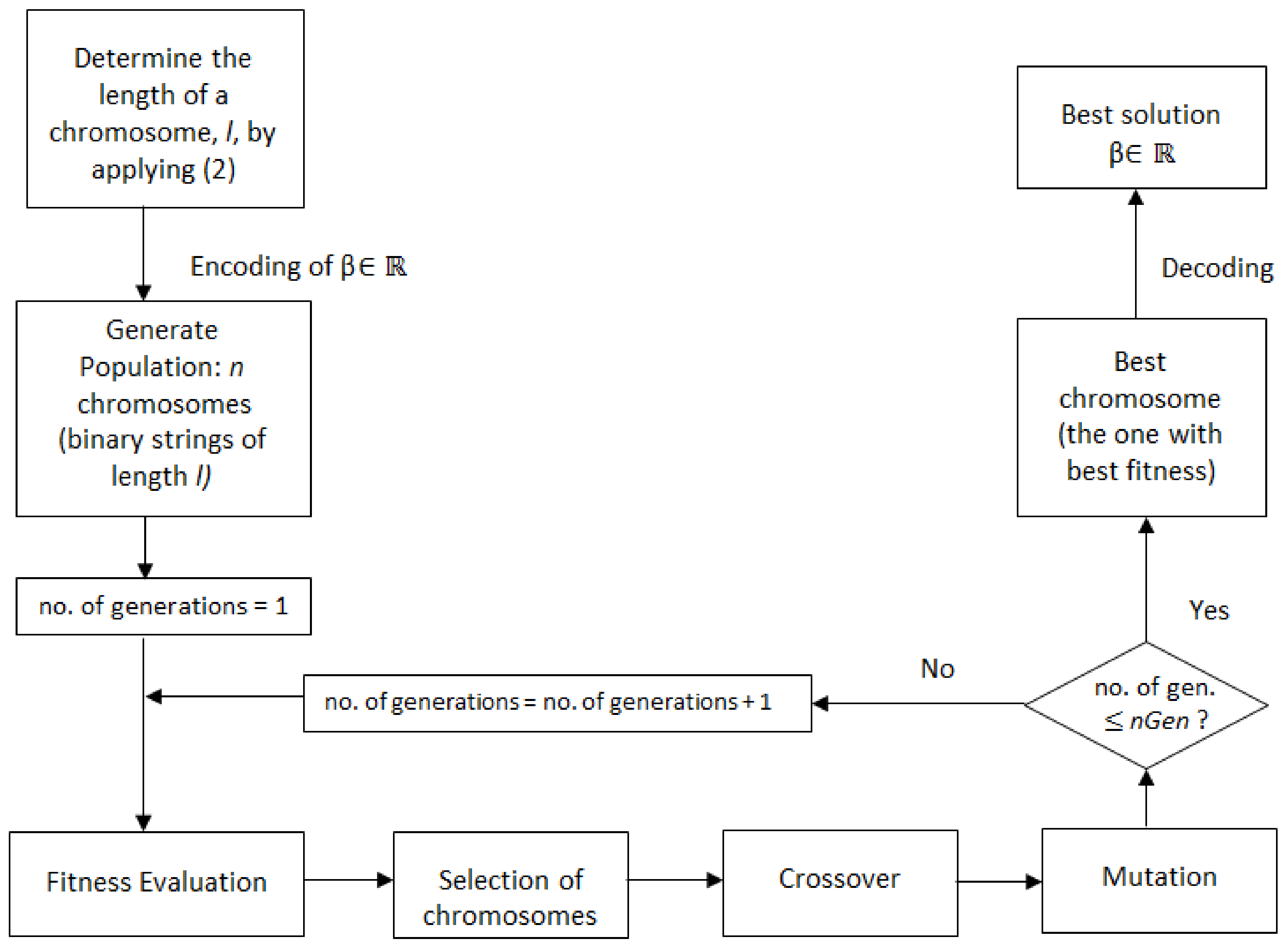
In this context, this article proposes a new approach that optimizes the finding of the beta parameter of IDW. This is based on a genetic algorithm and finds a unique β for the entire study region, while the classical one determines different βs for different interpolated series. The algorithm is proposed in four scenarios crossover/mutation: single-point/uniform, single-point/swap, two-point/uniform, and two-point swap. Comparisons of its performances with those of the classical IDW (with β = 2 and the optimal beta found in our algorithm), ordinary kriging, and two versions of the optimized IDW by using Particle Swarm Optimization (OIDW) are also provided.
3. Results and Discussion
Firstly, we ran several tests to find the settings of control parameters that are most likely to produce the best results. We started with predefined values from the literature [
27,
28] for the stop condition (10 generations), crossover rate (0.75), and mutation rate (0.015). Then, we varied the population size (from 10 to 80, with a step of 5) and computed the fitness function’s corresponding values, run time, and β.
Table 1 shows the relationship between the fitness value and population size.
For each pair of operators (single-point/uniform, single-point/swap, two-point/uniform, two-point/swap), we chose the optimal population size to be the lowest value from which population growth does not significantly influence the modification of the fitness value. This is 45, 40, 30, and 35 individuals, respectively, and the fitness function value is 0.0317. The corresponding β values obtained in the four scenarios are 1.256, 1.372, 1.308, and 1.336, respectively. These results are highlighted in
Table 1.
Since we used a predefined number of generations as the stop condition, in the second stage, we had to determine its optimal value. To find it, for each pair of operators, we ran tests with several values of the number of generations, the population size previously estimated (45, 40, 30, 35, respectively—
Table 1), keeping the mutation rate set to 0.015, and the crossover rate set to 0.75.
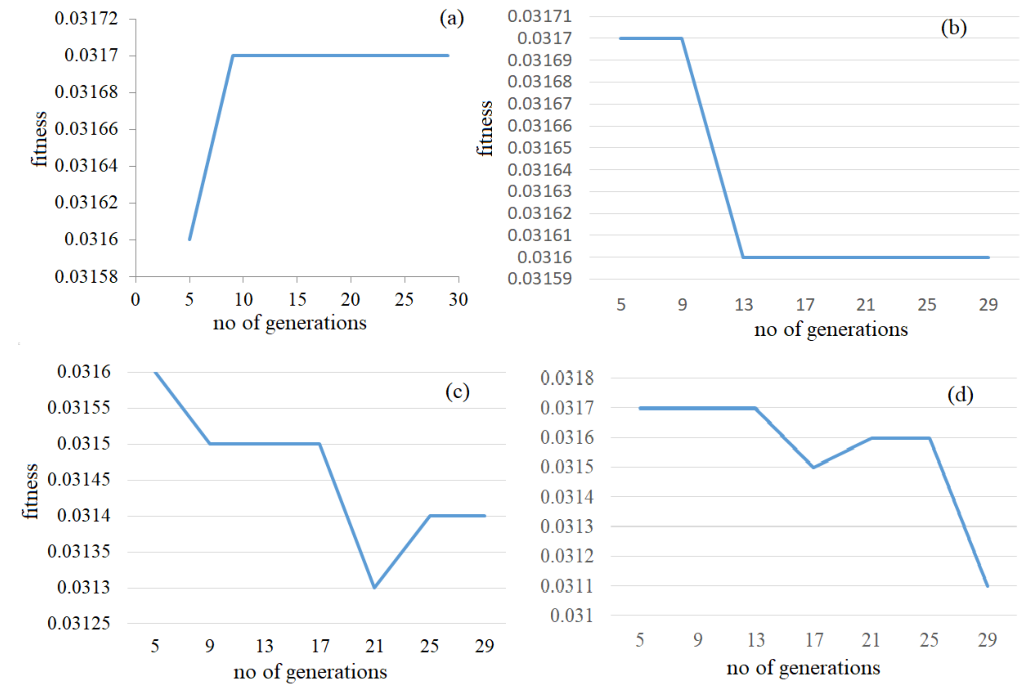
Table 2 and
Figure 3 show that the fitness value does not improve after a certain number of generations (which is the optimal number of generations).
Based on the highest fitness value, the optimum number of generations determined was nine for the single-point/uniform mutation scenario, whereas, for the other scenarios, the number of generations was five. The corresponding β-values obtained are 1.228, 1.242, 1.122, and 1.362, respectively (highlighted in
Table 2, together with the fitness and beta values). Since in our algorithm, β is represented by a chromosome, and several genetic operators have been used, different chromosomes (β) could produce the same fitness value.
The next step is the determination of the optimal crossover rate. For this aim, we ran the algorithm in each scenario with different values of the crossover rate (from 0.6 – value suggested in the literature to 0.95, with a step of 0.05), the population size and number of generations previously determined (45, 40, 30, and 35 individuals, respectively; 9, 5, 5, 5 generations, respectively), and the mutation rate kept to 0.015. We chose the optimal crossover rate for each pair of operators to be the value that gives the best (highest) fitness.
From
Table 3 it results that the best crossover rates are 0.8 when using a single-point/uniform scenario, 0.6 for single-point/swap, 0.75 for two-point/uniform, and 0.7 for two-point/swap. These values correspond to the highlighted sequences of values in
Table 3.
The last step was the determination of the best mutation rate. Therefore, we analyzed the impact the mutation rate has on the GA’s results. We considered the population size, the number of generations, and the crossover rates we established in previous stages, and we performed new tests aiming at detecting the value of the mutation rate. For example, for single-point uniform mutation, we took the population size = 45, the number of generations = 9, the crossover rate = 0.80, and ran the tests for a mutation rate from 0.02 to 0.1, with a step size of 0.01. For each pair of operators, we search the optimal mutation rate for which the fitness value evolves to a maximum along with the generations.
Table 4 contains the values of the fitness function obtained after running the algorithm in the four scenarios, with different mutation rates. For example, in
Table 4a we present the values of the fitness function obtained for each generation (from 1 to 9) and the mutation rates from 0.02 to 0.1, in the single-point crossover/uniform mutation scenario. The highest fitness value is obtained after nine generations in the single-point crossover/uniform mutation, with a mutation rate of 0.06 (the sixth column–the highlighted values).
In the single-point crossover/swap mutation (
Table 4b), the highest fitness value is 0.0315, obtained after 5 generations, with a mutation rate of 0.08 (the eighth column of
Table 4b). For the two-point crossover/uniform mutation and two-point crossover/swap mutation (
Table 4c,d), the best mutation rates are 0.04 and 0.05, respectively, and the corresponding value of the fitness function is 0.0313 (contained in the highlighted columns—the fourth and the fifth, respectively).
After setting the optimal parameters, determined in the previous stages, we finally ran the algorithm to determine the optimum beta parameters.
Table 5 summarizes the parameters used to implement the proposed genetic algorithm (columns 2–5), the fitness function obtained after running the algorithm with these parameters (column 6), the execution time (column 7), and the value obtained for the IDW’s parameter (last column).
Remark that the values of β are different when using different scenarios, even if the fitness value is the same. This is due to the specifics of the individuals’ selection and operations in GAs.
The lowest execution time (0.6188) is obtained when using the single-point/swap scenario and the highest one (10.5875 s) when using a two-point/swap procedure. Even if in the two-point/uniform case, the population size and the number of generations are the smallest, the execution time is high (the second-highest).
Table 6 contains the MSE and MAE for each station and the average (the last row of the table) computed after running the algorithm in each scenario. Comparing the MSEs in the two-point/swap and single-point/uniform (single-point/swap, and two-point/uniform) scenario, they are smaller in 70% (70%, 70%) cases, so our algorithm, in two-point/swap scenario, performs better in 70% cases compared to the other three scenarios. The MSEs’ averages (31.5874, 31.5306, 31.5188, 31.5153) are comparable, the smallest being obtained in the two-point/swap scenario, followed by the third one.
Comparing the MAEs in the two-point/swap and single-point/uniform (single-point/swap, and two-point/uniform) scenario, they are smaller in 80% (80%, 80%) cases, so our algorithm, in two-point/swap scenario, performs better in 80% cases compared to the other three scenarios. The MAEs’ averages (23.6352, 23.5542, 23.5308, 23.5228) are comparable, the smallest being obtained in the two-point/swap scenario, followed by the third one.
The corresponding values computed for beta in the best two cases are 1.042 (in two-point/swap) and 1.064 (in two-point/uniform).
For comparison reasons, we performed the classical IDW, with β = 2 (the value used in most applications) and β = 1.042. The MAE and MSE values computed for each station are presented in
Table 7.
Comparing the MSEs in the two-point/swap algorithm (
Table 6, column 8) with those from the IDW with β = 2 (
Table 7 column 2), they are smaller in 70% cases (the first four stations, the sixth, eighth, and ninth), so our algorithm performs better in 70% cases. Comparing the MSEs in the two-point/swap algorithm with those from the IDW with β = 1.042 (
Table 7 column 4), they are smaller in 60% cases (the second, third, fourth, sixth, eighth, and ninth stations), so our algorithm better performs in 60% cases.
In terms of the average MSEs, that in the two-point/swap approach is smaller than those of the IDW (β = 2), IDW (β = 1.042), and slightly higher than in KG (
Table 7, the last column). Still, our approach is preferable against KG since it is difficult to determine the kriging parameters, requiring special knowledge of geostatistics.
The MAEs in the two-point/swap algorithm are smaller than those from the IDW with β = 2, in 80% cases (all, but the first and sixth station), and comparable for the first station.
The MAEs in the two-point/swap algorithm are smaller than those from the IDW (β = 1.042), they in 60% cases (all, but the first and sixth station), and comparable for the first station.
The average MAE in the two-point/swap approach (23.5228) is significantly smaller than those in the IDW with β = 2 (26.90), and IDW with β = 1.042 (26.08).
From the computational viewpoint, the highest computational time in our experiment was 10.5875 (in the two-point scenario), while in the grid search to estimate beta with 3 decimals takes 60 seconds for each series, so, a total of 60*10 stations = 600 seconds, which is 56.67 times higher than in our approach.
The last two columns of in
Table 7 contains the MSE in the optimized IDW, denoted by OIDW [
18], in two scenarios, as described in [
18]—with different beta, found using a Particle Swarm Optimization (PSO) approach (column 7), or with a single best beta found by the same approach.
In term of MSE, our GA algorithm (
Table 7, column 8) performs better that OIDW (
Table 7, columns 7 and 8) in 80% of cases. Therefore, we can say that a significant improvement of the interpolation performances are obtained, that may reflect in the water management policy.


