
Evolution of Salinity and Water Table Level of the Phreatic Coastal Aquifer of the Emilia Romagna Region (Italy)

 ,
, 


Abstract
:1. Introduction
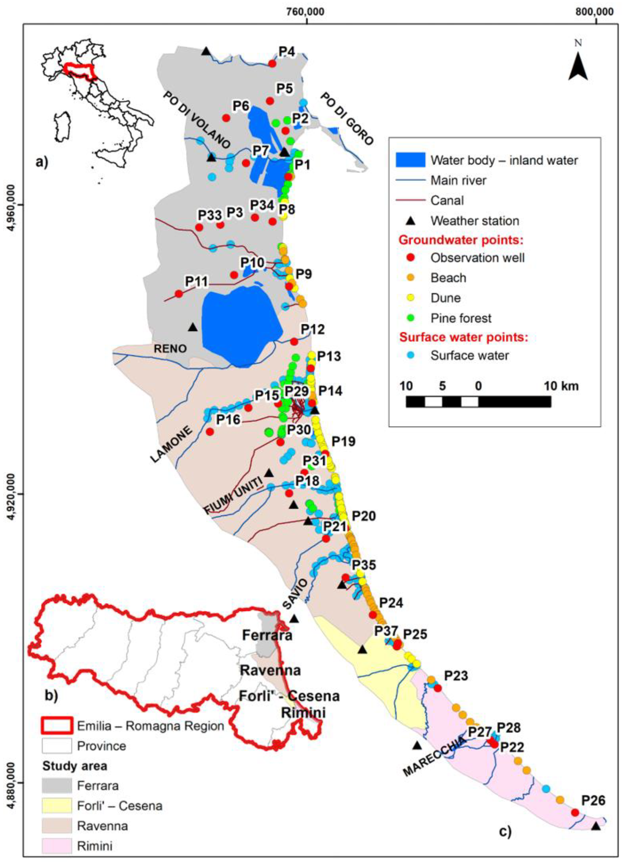
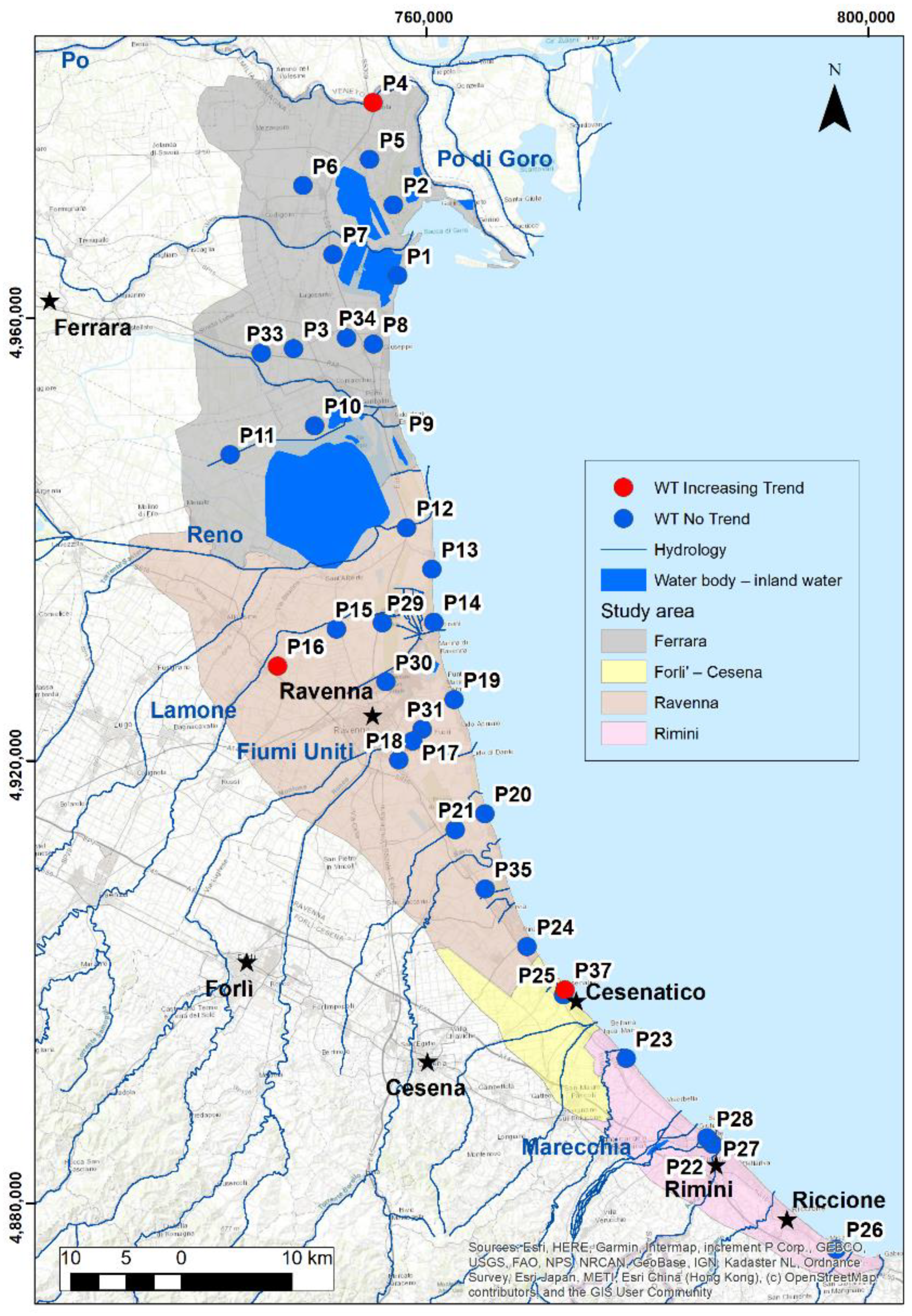
1.1. Study Area
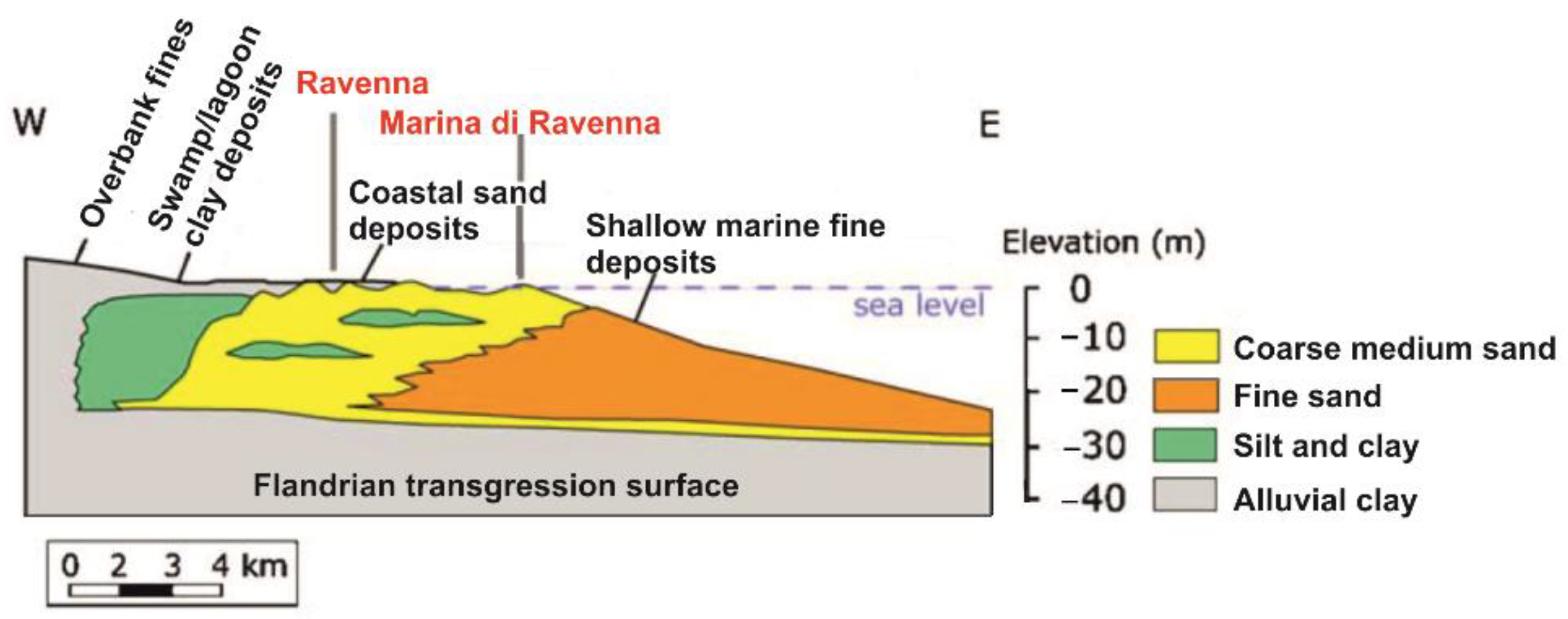
1.2. Hydrogeological Characterization
2. Methodology
2.1. Data Collection
2.2. Statistical Analysis
2.3. Spatial Analysis
- The predictions are unbiased when the MSE is close to 0;
- The standard errors are accurate when the RMSSE is close to 1;
- The predictions do not deviate much from the measured values, where the RMSE and ASE are as small as possible;
- Moreover, when ASE values are close to the RMSE from cross-validation, we can be confident that the model is appropriate.
3. Results
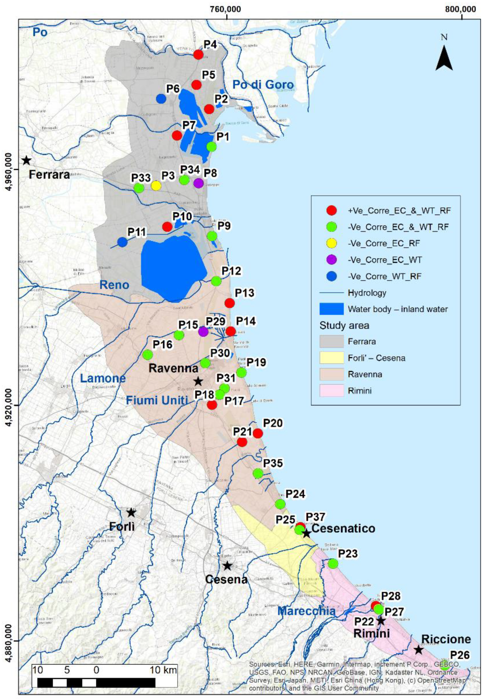
3.1. Correlation Analysis
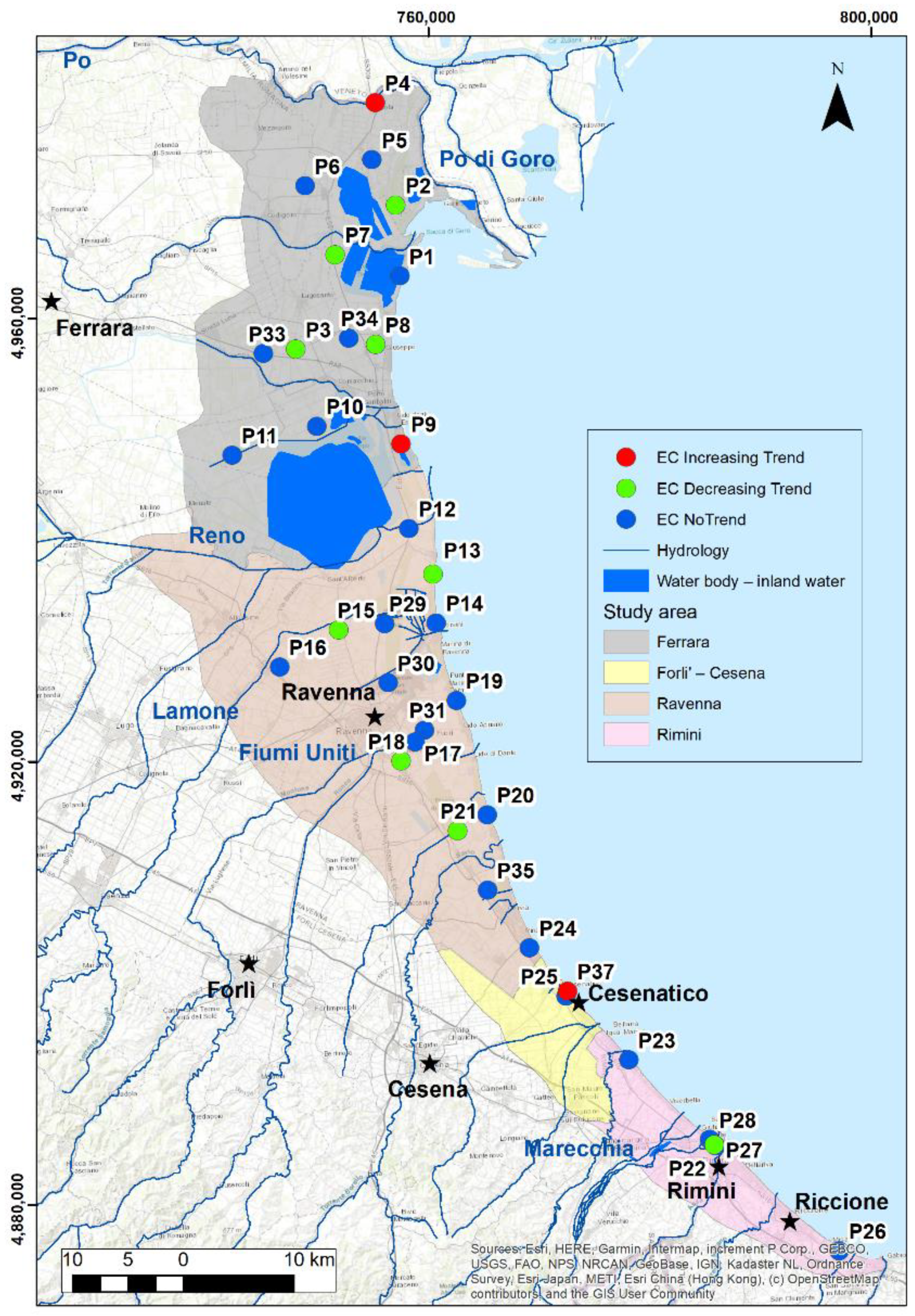
3.2. Trend Analysis
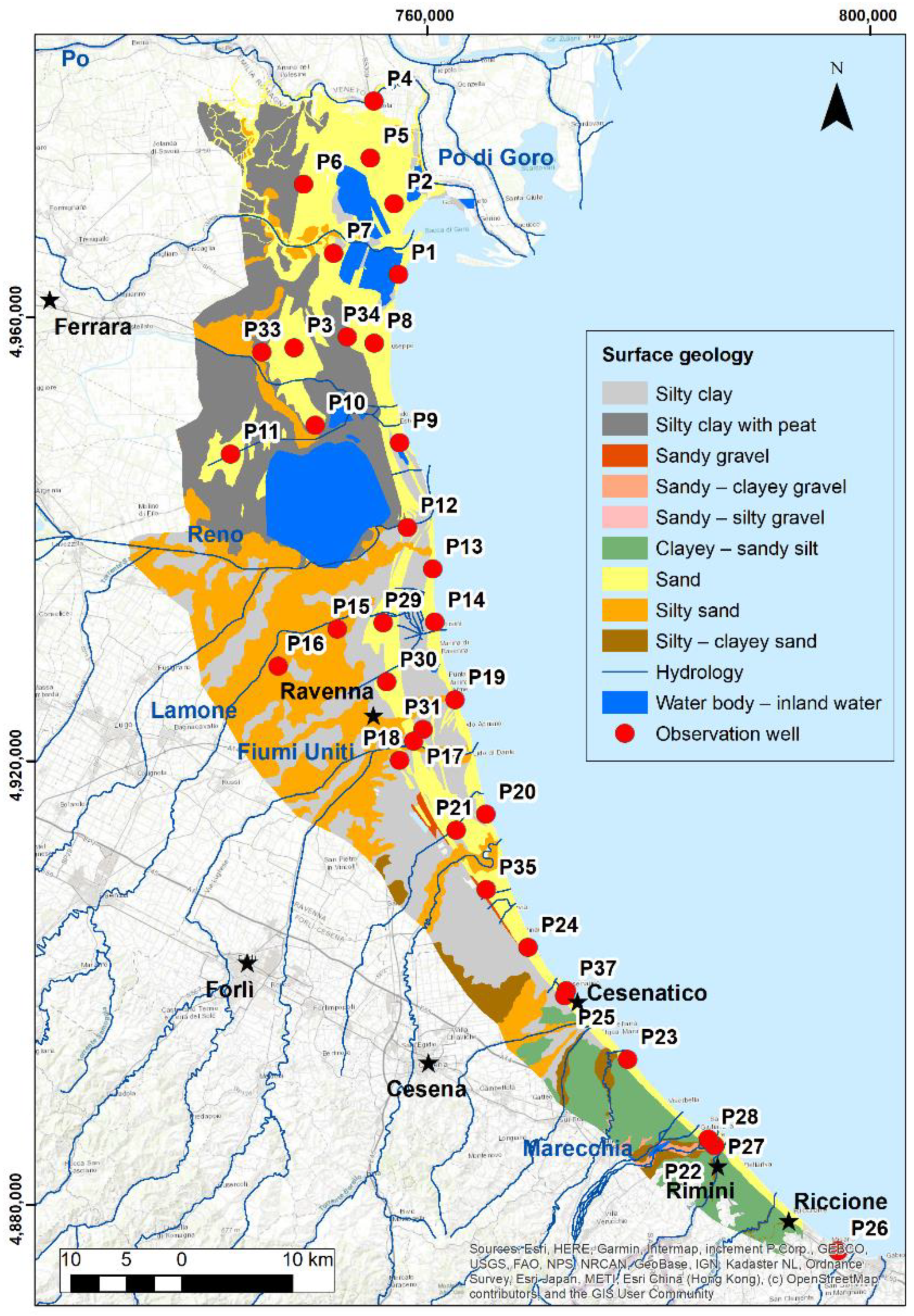
3.3. Surface Geology
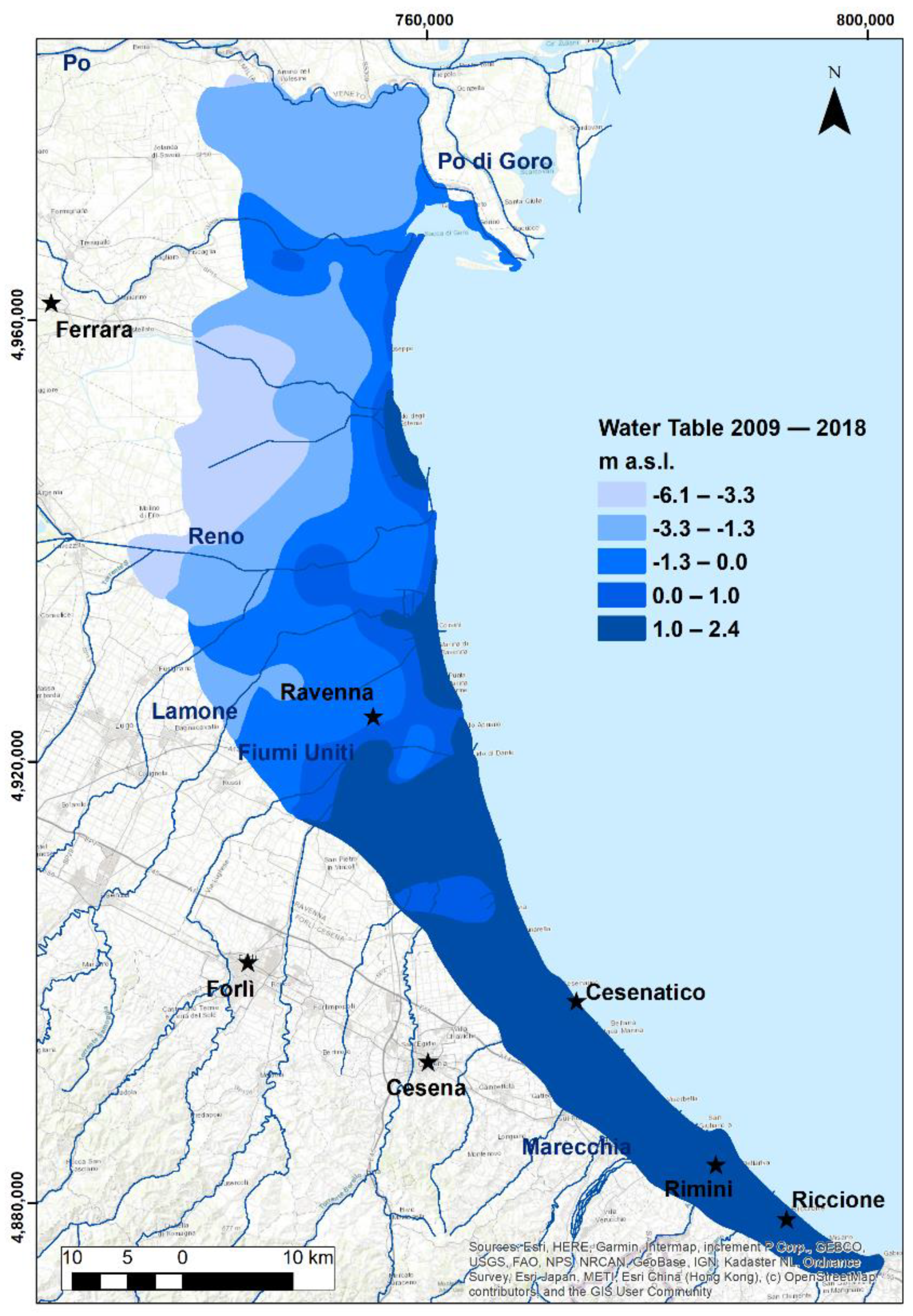
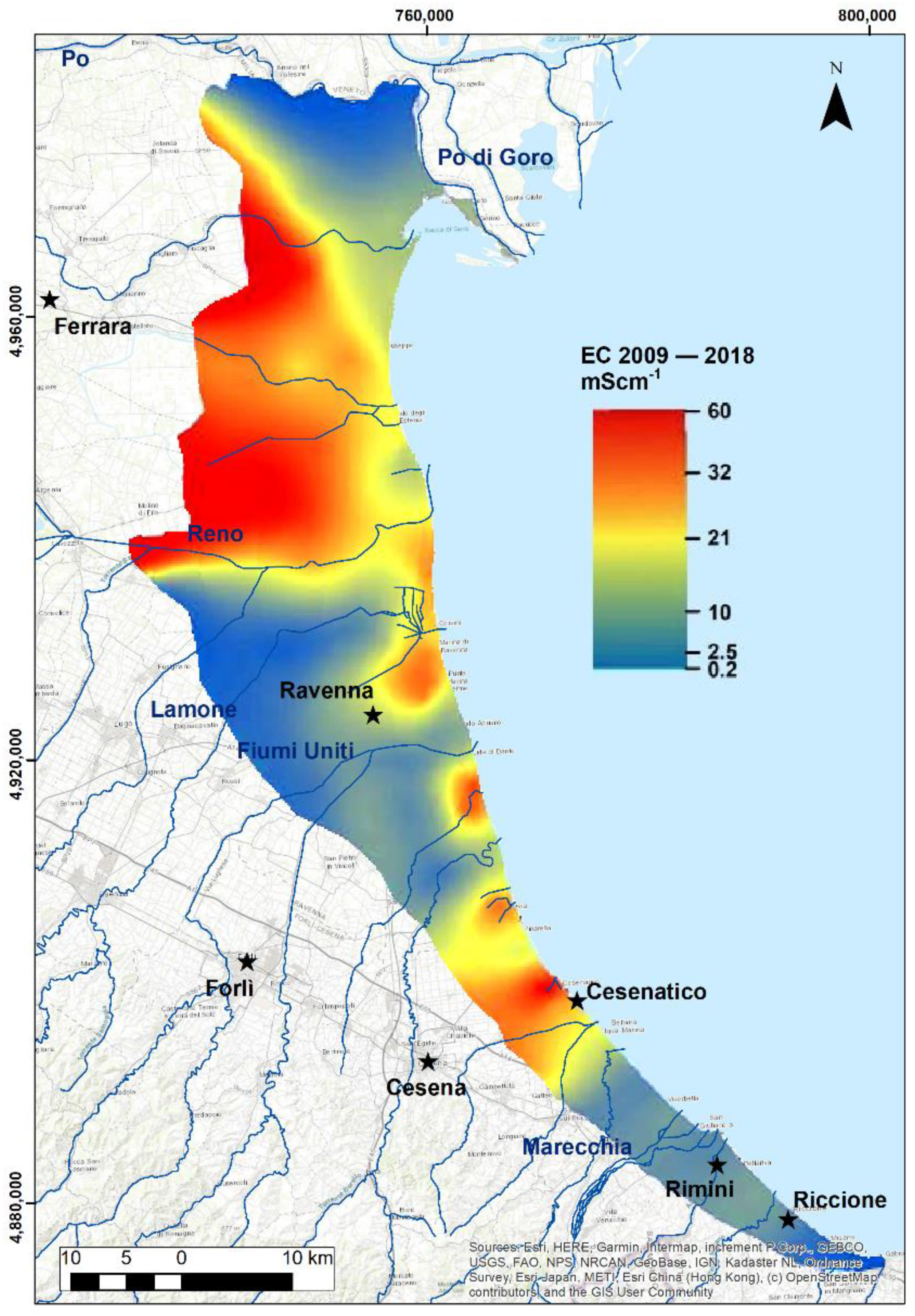
3.4. Spatial Analysis of Water Table Level and Electrical Conductivity
4. Discussion
4.1. Correlations and Statistical Analysis
4.2. Water Table Map
4.3. EC Distribution Map
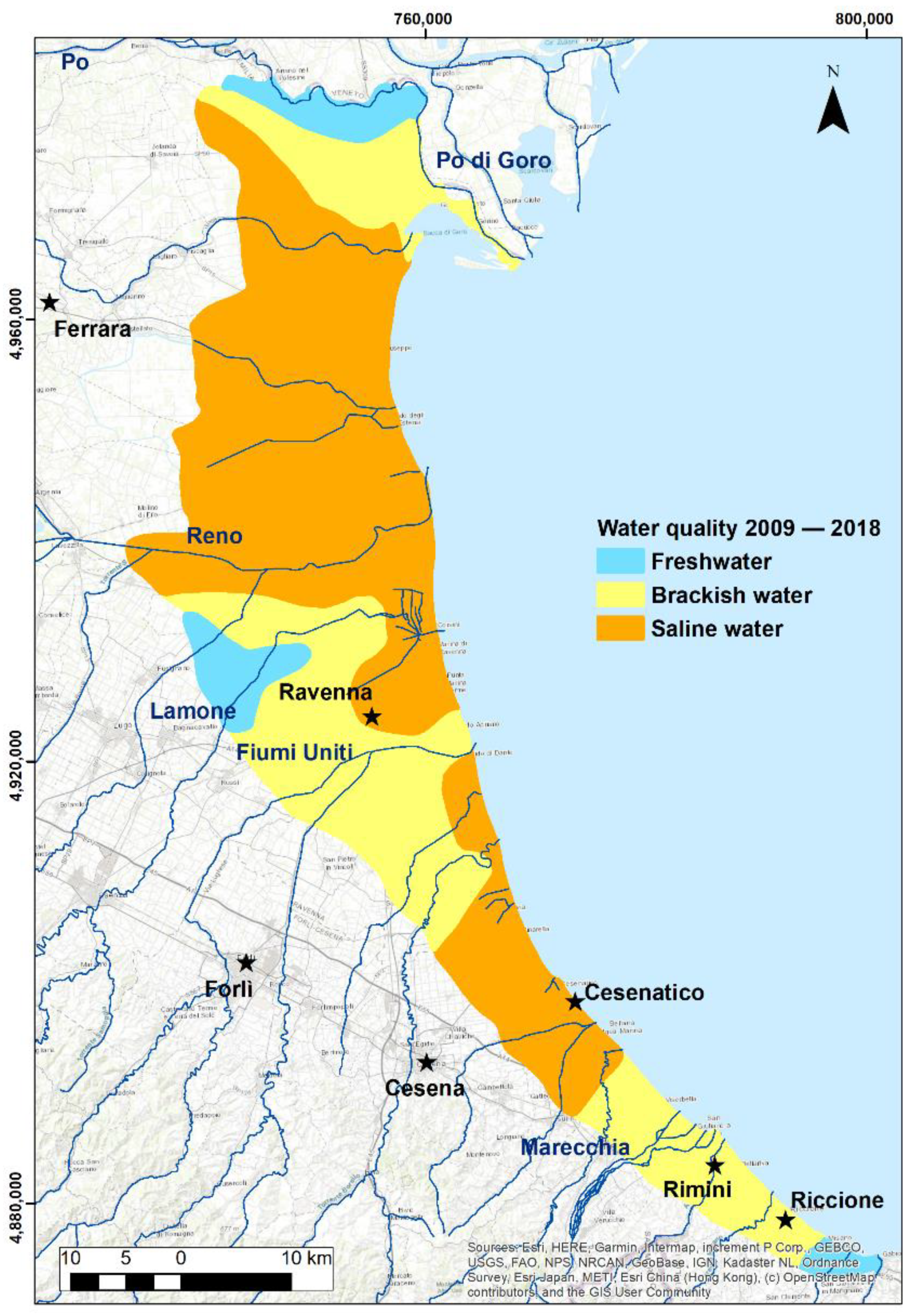
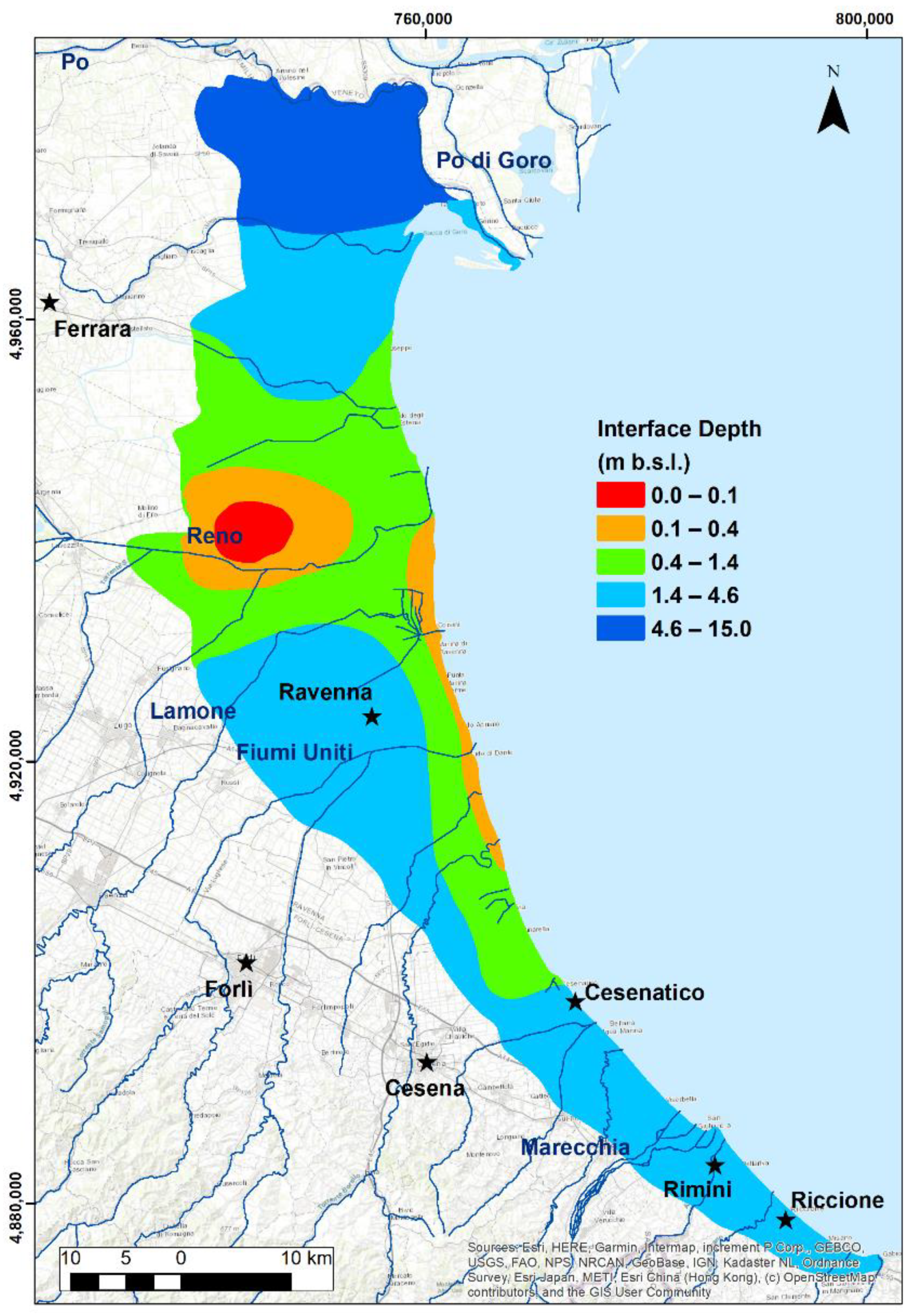
4.4. Water Quality Map and Freshwater–Saltwater Interface
5. Conclusions
Supplementary Materials
Author Contributions
Funding
Acknowledgments
Conflicts of Interest
References
- Neumann, B.; Ott, K.; Kenchington, R. Strong sustainability in coastal areas: A conceptual interpretation of SDG 14. Sustain. Sci. 2017, 12, 1019–1035. [Google Scholar] [CrossRef] [PubMed] [Green Version]
- Kumar, C. Climate change and its impact on groundwater resources. Int. J. Eng. Sci. 2012, 1, 43–60. [Google Scholar]
- Post, V.E.A.; Eichholz, M.; Brentführer, R. Groundwater Management in Coastal Zones; Bundesanstalt für Geowissenschaften und Rohstoffe (BGR): Hannover, Germany, 2018; p. 107. [Google Scholar]
- Ericson, J.P.; Vörösmarty, C.J.; Dingman, S.L.; Ward, L.G.; Meybeck, M. Effective sea-level rise and deltas: Causes of change and human dimension implications. Glob. Planet. Chang. 2006, 50, 63–82. [Google Scholar] [CrossRef]
- Custodio, E.; Bruggeman, G.A. Groundwater Problems in Coastal Areas; Studies and Reports in Hydrology 45; UNESCO: París, France; 596p.
- Vengosh, A. Salinization and Saline Environments. In Treatise on Geochemistry, 2nd ed.; Elsevier: Amsterdam, The Netherlands, 2014; pp. 325–378. [Google Scholar] [CrossRef]
- Antonellini, M.; Mollema, P.; Giambastiani, B.M.S.; Bishop, K.; Caruso, L.; Minchio, A.; Pellegrini, L.; Sabia, M.; Ulazzi, E.; Gabbianelli, G. Salt water intrusion in the coastal aquifer of the southern Po Plain, Italy. Hydrogeol. J. 2008, 16, 1541–1556. [Google Scholar] [CrossRef]
- Antonellini, M.; Allen, D.M.; Mollema, P.N.; Capo, D.; Greggio, N. Groundwater freshening following coastal progradation and land reclamation of the Po Plain, Italy. Hydrogeol. J. 2015, 23, 1009–1026. [Google Scholar] [CrossRef]
- Colombani, N.; Mastrocicco, M.; Giambastiani, B.M.S. Predicting Salinization Trends in a Lowland Coastal Aquifer: Comacchio (Italy). Water Resour. Manag. 2015, 29, 603–618. [Google Scholar] [CrossRef]
- Giambastiani, B.M.S.; Antonellini, M.; Essink, G.O.; Stuurman, R.J. Saltwater intrusion in the unconfined coastal aquifer of Ravenna (Italy): A numerical model. J. Hydrol. 2007, 340, 91–104. [Google Scholar] [CrossRef]
- Giambastiani, B.M.S.; Colombani, N.; Mastrocicco, M.; Fidelibus, M.D. Characterization of the lowland coastal aquifer of Comacchio (Ferrara, Italy): Hydrology, hydrochemistry and evolution of the system. J. Hydrol. 2013, 501, 35–44. [Google Scholar] [CrossRef]
- Greggio, N.; Mollema, P.N.; Antonellini, M.; Gabbianelli, G. Irrigation Management in Coastal Zones to Prevent Soil and Groundwater Salinization. In Resource Management for Sustainable Agriculture; Abrol, V., Ed.; IntechOpen: London, UK, 2012. [Google Scholar] [CrossRef] [Green Version]
- Cozzolino, D.; Greggio, N.; Antonellini, M.; Giambastiani, B.M.S. Natural and anthropogenic factors affecting freshwater lenses in coastal dunes of the Adriatic coast. J. Hydrol. 2017, 551, 804–818. [Google Scholar] [CrossRef]
- Giambastiani, B.M.S.; Macciocca, V.R.; Molducci, M.; Antonellini, M. Factors Affecting Water Drainage Long-Time Series in the Salinized Low-Lying Coastal Area of Ravenna (Italy). Water 2020, 12, 256. [Google Scholar] [CrossRef] [Green Version]
- Mollema, P.N.; Antonellini, M.; Dinelli, E.; Gabbianelli, G.; Greggio, N.; Stuyfzand, P.J. Hydrochemical and physical processes influencing salinization and freshening in Mediterranean low-lying coastal environments. Appl. Geochem. 2013, 34, 207–221. [Google Scholar] [CrossRef]
- Antonellini, M.; Mollema, P.N. Impact of groundwater salinity on vegetation species richness in the coastal pine forests and wetlands of Ravenna, Italy. Ecol. Eng. 2010, 36, 1201–1211. [Google Scholar] [CrossRef]
- Mollema, P.N.; Antonellini, M.; Gabbianelli, G.; Laghi, M.; Marconi, V.; Minchio, A. Climate and water budget change of a Mediterranean coastal watershed, Ravenna, Italy. Environ. Earth Sci. 2012, 65, 257–276. [Google Scholar] [CrossRef]
- Laghi, M.; Mollema, P.N.; Antonellini, M. The Influence of River Bottom Topography on Salt Water Encroachment Along the Lamone River (Ravenna, Italy), and Implications for the Salinization of the Adjacent Coastal Aquifer. In Proceedings of the World Environmental and Water Resources Congress 2010: Challenges of Change, Providence, RI, USA, 16–20 May 2010; ASCE, Ed.; pp. 1124–1135. [Google Scholar]
- Rivière, A.; Gonçalvès, J.; Jost, A.; Font, M. Experimental and numerical assessment of transient stream–Aquifer exchange during disconnection. J. Hydrol. 2014, 517, 574–583. [Google Scholar] [CrossRef] [Green Version]
- Bonzi, L.; Calabrese, L.; Severi, P.; Vincenzi, V. L’Acquifero Freatico Costiero della Regione Emilia-Romagna: Modello Geologico e Stato di Salinizzazione. Il Geologo dell’Emilia-Romagna 2010, 39, 21–34. [Google Scholar]
- Amorosi, A.; Colalongo, M.I.; Pasini, G.; Preti, D. Sedimentary response to Late Quaternary sea-level changes in the Romagna coastal plain (northern Italy). Sedimentology 1999, 46, 99–121. [Google Scholar] [CrossRef]
- Bondesan, M.; Favero, V.; Viñals, M.J. New evidence on the evolution of the Po-delta coastal plain during the Holocene. Quat. Int. 1995, 29, 105–110. [Google Scholar] [CrossRef]
- Amorosi, A.; Centineo, M.C.; Dinelli, E.; Lucchini, F.; Tateo, F. Geochemical and mineralogical variations as indicators of provenance changes in Late Quaternary deposits of SE Po Plain. Sediment. Geol. 2002, 151, 273–292. [Google Scholar] [CrossRef]
- Campo, B.; Amorosi, A.; Vaiani, S.C. Sequence stratigraphy and late Quaternary paleoenvironmental evolution of the Northern Adriatic coastal plain (Italy). Palaeogeogr. Palaeoclim. Palaeoecol. 2017, 466, 265–278. [Google Scholar] [CrossRef]
- Mann, H.B. Nonparametric tests against trend. Econometrica 1945, 13, 245–259. [Google Scholar] [CrossRef]
- Kendall, M.G.; Gibbons, J.D. Rank Correlation Methods (Charles Griffin Book Series); Oxford University Press: Oxford, UK, 1990; p. 272. [Google Scholar]
- Sen, P.K. Estimates of the regression coefficient based on Kendall’s Tau. J. Am. Stat. Assoc. 1968, 63, 1379–1389. [Google Scholar] [CrossRef]
- Gibbons, R.D.; Bhaumik, D.K.; Aryal, S. Statistical Methods for Groundwater Monitoring; John Wiley & Sons: Hoboken, NJ, USA, 2009; p. 400. [Google Scholar]
- Gilbert, R.O. Statistical Methods for Environmental Pollution Monitoring; Van Nostrand Reinhold Co: New York, NY, USA, 1987; p. 336. [Google Scholar]
- Yue, S.; Pilon, P.; Phinney, B.; Cavadias, G. The influence of autocorrelation on the ability to detect trend in hydrological series. Hydrol. Process. 2002, 16, 1807–1829. [Google Scholar] [CrossRef]
- Salmi, T.; Määttä, A.; Anttila, P.; Ruoho-Airola, T.; Amnell, T. Detecting Trends of Annual Values of Atmospheric Pollutants by the Mann-Kendall Test and Sen’s Slope Estimates: The Excel Template Application MAKESENS; Finnish Meteorological Institute: Helsinki, Finland, 2002; p. 35. [Google Scholar]
- McBean, E.; Motiee, H. Assessment of impact of climate change on water resources: A long term analysis of the Great Lakes of North America. Hydrol. Earth Syst. Sci. 2008, 12, 239–255. [Google Scholar] [CrossRef] [Green Version]
- Johnston, K.; Hoef, J.M.V.; Krivoruchko, K.; Lucas, N. Using ArcGIS Geostatistical Analyst; ESRI: Redlands, CA, USA, 2001; p. 307. [Google Scholar]
- Berke, O. Estimation and Prediction in the Spatial Linear Model. Water Air Soil Pollut. 1999, 110, 215–237. [Google Scholar] [CrossRef]
- Mustapha, A. Detecting surface water quality trends using Mann-Kendall tests and Sen’s slope estimates. IJAIR 2013, 108–114. [Google Scholar]
- Obaje, N.G. Geology and Mineral Resources of Nigeria; Series: Lecture Notes in Earth Sciences; Springer: Berlin/Heidelberg, Germany, 2009; Volume 120. [Google Scholar] [CrossRef]
- Cay, T.; Uyan, M. Spatial and temporal groundwater level variation geostatistical modeling in the city of Konya, Turkey. Water Environ. Res. 2009, 81, 2460–2470. [Google Scholar] [CrossRef] [PubMed]
- Giambastiani, B.M.S.; Greggio, N.; Nobili, G.; Dinelli, E.; Antonellini, M. Forest fire effects on groundwater in a coastal aquifer (Ravenna, Italy). Hydrol. Process. 2018, 32, 2377–2389. [Google Scholar] [CrossRef]
- Greggio, N.; Giambastiani, B.M.S.; Balugani, E.; Amaini, C.; Antonellini, M. High-Resolution Electrical Resistivity Tomography (ERT) to Characterize the Spatial Extension of Freshwater Lenses in a Salinized Coastal Aquifer. Water 2018, 10, 1067. [Google Scholar] [CrossRef] [Green Version]
- Piccinini, L.; Vincenzi, V.; Gargini, A. Monitoraggio di flusso a densità variabile di un acquifero freatico salinizzato. Giornale Geologia Applicata 2008, 9, 249–261. [Google Scholar]
- Legislative Decree. Attuazione della direttiva 98/83/CE relativa alla qualità delle acque destinate al consumo umano. Implement. Dir. 2001, 98, 83. [Google Scholar]
- Rose, D.A.; Konukcu, F.; Gowing, J.W. Effect of watertable depth on evaporation and salt accumulation from saline groundwater. Soil Res. 2005, 43, 565. [Google Scholar] [CrossRef]
- Boonstra, J.; Bhutta, M.N. Groundwater recharge in irrigated agriculture: The theory and practice of inverse modelling. J. Hydrol. 1996, 174, 357–374. [Google Scholar] [CrossRef]
- Bouwer, H. Chapter 24—Artificial Recharge of Groundwater: Systems, Design, and Management. In Hydraulic Design Handbook; Mays, L.W., Ed.; McGraw-Hill: New York, NY, USA, 1999. [Google Scholar]
- Schneider, J.C.; Kruse, S.E. Assessing selected natural and anthropogenic impacts on freshwater lens morphology on small barrier Islands: Dog Island and St. George Island, Florida, USA. Hydrogeol. J. 2006, 14, 131–145. [Google Scholar] [CrossRef]
- Vandenbohede, A.; Mollema, P.N.; Greggio, N.; Antonellini, M. Seasonal dynamic of a shallow freshwater lens due to irrigation in the coastal plain of Ravenna, Italy. Hydrogeol. J. 2014, 22, 893–909. [Google Scholar] [CrossRef]
- ISPRA. Variazioni e Tendenze Degli Estremi di Temperatura e Precipitazione in Italia. Stato dell’Ambiente. 2013. Available online: https://www.isprambiente.gov.it/it/pubblicazioni/stato-dellambiente/variazioni-e-tendenze-degli-estremi-di-temperatura-e-precipitazione-in-italia (accessed on 15 January 2021).
- Cervi, F.; Nistor, M.-M. High Resolution of Water Availability for Emilia-Romagna Region over 1961–2015. Adv. Meteorol. 2018, 2018, 2489758. [Google Scholar] [CrossRef]
- Mollema, P.N.; Antonellini, M.; Gabbianelli, G.; Galloni, E. Water budget management of a coastal pine forest in a Mediterranean catchment (Marina Romea, Ravenna, Italy). Environ. Earth Sci. 2013, 68, 1707–1721. [Google Scholar] [CrossRef]


| Piezometer | Statistical Summary | Mann–Kendall Test | Sen’s Slope EC (mScm−1 year−1) | Trend | |||||
|---|---|---|---|---|---|---|---|---|---|
| Min. | Median | Mean | Max. | Z | S | Sign. | |||
| P1 | 0.87 | 38.91 | 35.82 | 52.33 | −0.45 | −16.00 | * | −0.27 | Decreasing |
| P2 | 16.30 | 21.28 | 20.87 | 23.80 | −2.18 | −68.00 | S | −0.12 | Decreasing |
| P3 | 2.81 | 10.95 | 10.82 | 17.60 | −2.17 | −68.00 | S | −0.31 | Decreasing |
| P4 | 0.40 | 0.50 | 0.49 | 0.90 | 2.18 | 62.00 | S | 0.01 | Increasing |
| P5 | 1.10 | 2.15 | 2.39 | 5.80 | 0.36 | 12.00 | * | 0.01 | Increasing |
| P6 | 0.60 | 0.80 | 0.85 | 1.10 | −0.86 | −11.00 | * | 0.00 | No trend |
| P7 | 1.21 | 2.10 | 2.06 | 3.50 | −2.30 | −66.00 | S | −0.05 | Decreasing |
| P8 | 18.50 | 34.20 | 35.72 | 52.30 | −3.64 | −105.00 | S | −1.34 | Decreasing |
| P9 | 0.50 | 1.50 | 1.65 | 3.77 | 2.31 | 72.00 | S | 0.06 | Increasing |
| P10 | 26.80 | 42.80 | 39.46 | 47.76 | 0.67 | 20.00 | * | 0.12 | Increasing |
| P11 | 31.10 | 35.30 | 36.65 | 46.50 | 0.70 | 10.00 | * | 0.50 | Increasing |
| P12 | 19.05 | 28.90 | 29.59 | 40.30 | −0.86 | −20.00 | * | −0.23 | Decreasing |
| P13 | 31.20 | 39.45 | 39.26 | 44.30 | −2.35 | −63.00 | S | −0.33 | Decreasing |
| P14 | 12.23 | 15.80 | 15.10 | 16.30 | −1.07 | −27.00 | * | −0.02 | Decreasing |
| P15 | 5.25 | 16.13 | 14.17 | 24.31 | −2.43 | −60.00 | S | −0.80 | Decreasing |
| P16 | 7.23 | 9.16 | 9.06 | 10.10 | −1.94 | −44.00 | * | −0.07 | Decreasing |
| P17 | 4.04 | 10.04 | 9.71 | 16.92 | 0.30 | 7.00 | * | 0.13 | Increasing |
| P18 | 14.28 | 17.99 | 17.30 | 18.89 | −3.56 | −80.00 | S | −0.11 | Decreasing |
| P19 | 23.07 | 30.81 | 30.56 | 41.04 | −0.37 | −10.00 | * | −0.16 | Decreasing |
| P20 | 21.95 | 27.61 | 27.25 | 33.25 | 1.06 | 29.00 | * | 0.18 | Increasing |
| P21 | 9.52 | 13.83 | 13.32 | 15.98 | −3.27 | −67.00 | S | −0.28 | Decreasing |
| P22 | 12.04 | 16.50 | 16.51 | 21.14 | −2.80 | −75.00 | S | −0.40 | Decreasing |
| P23 | 1.22 | 1.39 | 1.51 | 2.34 | −1.36 | −34.00 | * | −0.02 | Decreasing |
| P24 | 0.99 | 1.83 | 1.82 | 2.38 | −1.53 | −35.00 | * | −0.03 | Decreasing |
| P25 | 1.09 | 1.75 | 1.89 | 3.60 | −0.30 | −9.00 | * | −0.01 | Decreasing |
| P26 | 1.15 | 1.36 | 1.40 | 1.93 | −0.73 | −8.00 | * | −0.02 | Decreasing |
| P27 | 1.35 | 1.57 | 1.55 | 1.71 | 1.48 | 31.00 | * | 0.01 | Increasing |
| P28 | 1.25 | 1.41 | 1.47 | 1.82 | 0.55 | 12.00 | * | 0.01 | Increasing |
| P29 | 3.09 | 5.66 | 5.32 | 5.86 | 1.80 | 13.00 | * | 0.09 | Increasing |
| P30 | 6.83 | 8.27 | 9.32 | 11.89 | −1.20 | −9.00 | * | −0.62 | Decreasing |
| P31 | 2.16 | 19.71 | 16.71 | 26.05 | −1.88 | −11.00 | * | −2.60 | Decreasing |
| P33 | 12.24 | 35.07 | 33.20 | 41.61 | −0.30 | −3.00 | * | −0.92 | Decreasing |
| P34 | 32.24 | 40.70 | 39.81 | 45.14 | 0.15 | 2.00 | * | 0.01 | Increasing |
| P35 | 0.88 | 1.21 | 1.36 | 1.87 | −1.22 | −6.00 | * | −0.25 | Decreasing |
| P37 | 16.09 | 32.81 | 30.48 | 38.26 | 2.75 | 46.00 | S | 1.01 | Increasing |
| Piezometer | Statistical Summary | Mann–Kendall Test | Sen’s Slope WT (m year−1) | Trend | |||||
|---|---|---|---|---|---|---|---|---|---|
| Min. | Median | Mean | Max. | Z | S | Sign. | |||
| P1 | −1.25 | −0.85 | 0.87 | 0.49 | 0.30 | 11.00 | * | 0.00 | No trend |
| P2 | −2.53 | −1.96 | −1.94 | −1.48 | 0.13 | 5.00 | * | 0.00 | No trend |
| P3 | −3.26 | −2.70 | −2.76 | −2.47 | −1.40 | −44.00 | * | −0.01 | Falling |
| P4 | −3.25 | −2.89 | −2.86 | −2.39 | 2.67 | 83.00 | S | 0.02 | Rising |
| P5 | −2.47 | −1.95 | −1.96 | −1.63 | −1.30 | −41.00 | * | −0.01 | Falling |
| P6 | −2.47 | −2.29 | −2.28 | −2.10 | −0.16 | −3.00 | * | −0.01 | Falling |
| P7 | −3.00 | −2.30 | −2.37 | −2.03 | −0.95 | −28.00 | * | −0.01 | Falling |
| P8 | −1.95 | −1.58 | −1.58 | −1.27 | 0.32 | 10.00 | * | 0.01 | Rising |
| P9 | −0.24 | 0.40 | 0.36 | 1.15 | 0.20 | 7.00 | * | 0.00 | No trend |
| P10 | −4.21 | −3.84 | −3.84 | −3.59 | 1.05 | 31.00 | * | 0.01 | Rising |
| P11 | −5.26 | −5.10 | −5.04 | −4.15 | −0.39 | −6.00 | * | −0.01 | Falling |
| P12 | −1.53 | −1.21 | −1.06 | −0.48 | 1.00 | 23.00 | * | 0.02 | Rising |
| P13 | 0.24 | 0.44 | 0.53 | 1.29 | −1.82 | −48.00 | * | −0.02 | Falling |
| P14 | −0.47 | −0.07 | 0.12 | 0.93 | 0.37 | 10.00 | * | 0.01 | Rising |
| P15 | −1.22 | −0.54 | −0.53 | 0.14 | 0.83 | 21.00 | * | 0.03 | Rising |
| P16 | −1.83 | −1.44 | −1.33 | −0.34 | 2.03 | 46.00 | S | 0.03 | Rising |
| P17 | −1.46 | −0.83 | −0.91 | −0.31 | 1.19 | 25.00 | * | 0.03 | Rising |
| P18 | −1.90 | −1.51 | −1.27 | −0.50 | 1.00 | 23.00 | * | 0.02 | Rising |
| P19 | 0.42 | 0.68 | 0.78 | 1.28 | 0.13 | 4.00 | * | 0.00 | No trend |
| P20 | −0.12 | 0.58 | 0.64 | 1.23 | 0.15 | 5.00 | * | 0.00 | No trend |
| P21 | −0.35 | −0.15 | −0.12 | 0.10 | −0.40 | −9.00 | * | −0.01 | Falling |
| P22 | 0.57 | 0.72 | 0.72 | 0.92 | 0.50 | 14.00 | * | 0.00 | No trend |
| P23 | −0.15 | 0.62 | 0.57 | 0.90 | 0.29 | 8.00 | * | 0.01 | Rising |
| P24 | −0.14 | 0.67 | 0.55 | 0.92 | 0.99 | 23.00 | * | 0.01 | Rising |
| P25 | 0.25 | 0.62 | 0.63 | 1.14 | 1.03 | 28.00 | * | 0.01 | Rising |
| P26 | 0.26 | 0.85 | 0.86 | 1.39 | 0.31 | 4.00 | * | 0.03 | Rising |
| P27 | 0.75 | 0.96 | 0.95 | 1.24 | −0.20 | −5.00 | * | 0.00 | No trend |
| P28 | −0.09 | 0.28 | 0.26 | 0.60 | 0.30 | 7.00 | * | 0.01 | Rising |
| P29 | −0.61 | −0.26 | −0.17 | 0.34 | −1.20 | −9.00 | * | −0.13 | Falling |
| P30 | −2.23 | −2.03 | −1.92 | −1.43 | 1.50 | 11.00 | * | 0.11 | Rising |
| P31 | −1.13 | −0.94 | −0.68 | 0.12 | 0.75 | 5.00 | * | 0.15 | Rising |
| P33 | −6.56 | −6.01 | −6.08 | −5.78 | 0.60 | 5.00 | * | 0.08 | Rising |
| P34 | −2.83 | −2.35 | −1.97 | 1.11 | −0.30 | −3.00 | * | 0.00 | No trend |
| P35 | −0.67 | −0.39 | −0.40 | −0.07 | 1.01 | 5.00 | * | 0.13 | Rising |
| P37 | −0.30 | 0.65 | 0.60 | 0.97 | 2.45 | 41.00 | S | 0.04 | Rising |
| Parameter | Season | Method | Best-Fit Model | ME | RMSE | MSE | RMSSE | ASE |
|---|---|---|---|---|---|---|---|---|
| Water Table Level (m) | 2009 to 2018 | Ordinary Kriging | Spherical | 0.004 | 0.63 | 0.006 | 1.30 | 0.50 |
| EC (mScm−1) | 2009 to 2018 | Ordinary Kriging | Spherical | 0.26 | 15.80 | 0.01 | 0.94 | 17.04 |
Publisher’s Note: MDPI stays neutral with regard to jurisdictional claims in published maps and institutional affiliations. |
© 2021 by the authors. Licensee MDPI, Basel, Switzerland. This article is an open access article distributed under the terms and conditions of the Creative Commons Attribution (CC BY) license (http://creativecommons.org/licenses/by/4.0/).
Share and Cite
Giambastiani, B.M.S.; Kidanemariam, A.; Dagnew, A.; Antonellini, M. Evolution of Salinity and Water Table Level of the Phreatic Coastal Aquifer of the Emilia Romagna Region (Italy). Water 2021, 13, 372. https://doi.org/10.3390/w13030372
Giambastiani BMS, Kidanemariam A, Dagnew A, Antonellini M. Evolution of Salinity and Water Table Level of the Phreatic Coastal Aquifer of the Emilia Romagna Region (Italy). Water. 2021; 13(3):372. https://doi.org/10.3390/w13030372
Chicago/Turabian StyleGiambastiani, Beatrice Maria Sole, Assaye Kidanemariam, Addisu Dagnew, and Marco Antonellini. 2021. "Evolution of Salinity and Water Table Level of the Phreatic Coastal Aquifer of the Emilia Romagna Region (Italy)" Water 13, no. 3: 372. https://doi.org/10.3390/w13030372
APA StyleGiambastiani, B. M. S., Kidanemariam, A., Dagnew, A., & Antonellini, M. (2021). Evolution of Salinity and Water Table Level of the Phreatic Coastal Aquifer of the Emilia Romagna Region (Italy). Water, 13(3), 372. https://doi.org/10.3390/w13030372