Article

Epiphyton in Agricultural Streams: Structural Control and Comparison to Epilithon

1
Department of Hydrology and Water Resources Management, Institute for Natural Resource Conservation, Kiel University, 24118 Kiel, Germany
2
Department of Biology, Aarhus University, Ole Worms Allé 1, 8000 Aarhus, Denmark
3
Department of Limnology and Water Technology, Faculty of Fisheries and Marine Sciences & Technology, University of Ruhuna, Matara 81000, Sri Lanka
4
Department of Geography and Spatial Information Techniques, Ningbo University, Ningbo 315211, China
5
Department of Bioscience, Aarhus University, Vejlsøvej 25, 8800 Silkeborg, Denmark
6
WATEC, Aarhus University Centre for Water Technology, Department of Biology, 8000 Aarhus, Denmark
*
Authors to whom correspondence should be addressed.
Water 2021, 13(23), 3443; https://doi.org/10.3390/w13233443
Submission received: 11 October 2021 / Revised: 17 November 2021 / Accepted: 1 December 2021 / Published: 4 December 2021
(This article belongs to the Special Issue Phytoplankton and Phytobenthos: From Freshwater to Marine Ecosystems)

Abstract

:
Stream biofilms play an important role in the structure, functioning, and integrity of agricultural streams. In many lowland streams, macrophyte vegetation is abundant and functions as an important substrate for biofilm (epiphyton) in addition to the gravel and stone substrate for epilithon on the stream bed. We expect that reach-scale habitat conditions in streams (e.g., nutrient availability, hydraulic conditions) affect the epiphyton and epilithon biomass and composition, and that this effect will be substrate-specific (macrophytes and stones). The objectives of our study were (i) to describe concurrent changes in epiphyton and epilithon biomass and composition over a year in agricultural streams, and (ii) to determine the substrate specific reach-scale habitat drivers for the epiphyton and epilithon structure. We monitored epiphyton and epilithon biofilm biomass and composition at three-week intervals and reach-scale environmental conditions daily during a year for two agricultural steams. The results showed that epiphyton and epilithon communities differed in biomass, having high substrate specific biomass in epilithon compared to epiphyton. Epiphyton was mainly composed of diatom and green algae, while cyanobacteria were more important in epilithon, and the diatom species composition varied between the two biofilm types. Epiphyton structural properties were less influenced by reach-scale hydrology and nutrient availability compared to epilithon. The overall explanatory power of the measured environmental variables was low, probably due to micro-scale habitat effects and interactive processes within stream biofilms. Knowledge of biofilm control in agricultural streams is important in order to improve management strategies, and future studies should improve the understanding of micro-scale habitat conditions, interactive relationships within biofilms and between the biofilm and the substrates.

1. Introduction

Stream biofilms play a unique and key role in aquatic ecosystems due to their involvement in biogeochemical cycles through primary production, ecosystem metabolism, nutrient uptake and trophic interactions [1,2]. Biofilms are complex in their structure and function, and are composed of autotrophic microalgae dominated by diatoms, green algae and cyanobacteria, as well as heterotrophic organisms such as bacteria, protozoa, and fungi [3]. Biofilm grows on various substrates in the stream, including macrophytes (epiphyton) and stone and gravel (epilithon), and their development is controlled by a complex array of factors and interactions [4] with irradiance, nutrient availability, physical disturbance and grazing being the most important [5].
Most studies on biofilm structure in lowland agricultural streams have been on epilithic biofilm, e.g., [6,7] and much less is known about the epiphytic biofilm, although we know it might be the primary site for microalgae growth in macrophyte-rich streams and may be the main contributor to reach-scale metabolism [8] and nutrient uptake [9]. Furthermore, macrophytes as biofilm substrate offer very different conditions for auto- and heterotrophic biofilm compared to gravel, and stones and the communities may therefore differ. First, macrophytes are organic substrates and thus may leach organic carbon [10,11] and nutrients [12,13,14]. Macrophytes may also exchange CO2 and O2 with epiphytic biofilm, as a product of photosynthesis and respiration [15]. In addition, internal biofilm recycling of nutrient and gas may occur [16] and affect both the biofilm and the host. Second, macrophytes grow as dense beds, creating a strong gradient in hydraulic conditions from the more exposed outside, to the inside with reduced hydraulic disturbance (i.e., reduced alternation in water velocity and turbulence) [17]. In contrast, nutrient and gas exchange in epilithic biofilm occur via the open stream water or internal recycling in the biofilm. Therefore, hydrological disturbance and resource availability can be very different for epiphytic and epilithic biofilm at a given time and the differences may vary with temporal changes in hydrology and resource availability in the streams on a daily and seasonal scale [18]. Ultimately, it may lead to structural differences in epiphyton and epilithon communities in terms of biomass and composition, driven by substrate-specific drivers.
Epilithon is typically dominated by firmly attached diatoms or green filamentous algae [19,20], but higher abundances of cyanobacteria may occur depending on the environmental conditions [21]. Diatoms are also considered to be the predominant group of algae in the epiphyton community [22,23], but the composition changes over seasons depending on both environmental conditions and the growth pattern of the host plant [23,24]. Some studies argue that epiphyton and epilithon diatom species composition is remarkably different, e.g., [17] while others state the opposite, e.g., [25]. Overall, nutrients such as phosphate (PO43−) and organic contaminants are the main drivers of diatom assemblages in streams, e.g., [6,26,27,28] and their composition can therefore be closely related to land use in the stream catchment and reach-scale habitat factors. Overall, Biggs [5], Biggs et al. [29,30] link reach-scale hydrological and hydraulic factors to periphyton abundance and composition. More specifically, Cantonati and Spitale [17] found that diatom species composition was predominantly driven by reach-scale temperature, water velocity, nitrate (NO3) and PO43− in both the epiphyton and epilithon in mountainous streams surrounded by a pristine environment, while Winter and Duthie [25] identified alkalinity, conductivity, suspended solids, and biological oxygen demand as the main drivers in streams surrounded by the mixed-land use of urban, agriculture and woodlands. One study with concurrent measurements of epiphyton and epilithon, [23] found that the species composition of epiphytic algae on Ranunculus sp. were overall similar to the epilithic algae species on stream bed gravel, and that the dominant species differed between the two substrata.
The objectives of our study were to further explore the epiphyton and epilithon community in streams (i) to describe concurrent changes of epiphyton and the epilithon biomass and composition during a year in agricultural streams, and (ii) to determine the substrate-specific reach-scale habitat drivers for the epiphyton and epilithon structure. We described epiphyton and epilithon composition in terms of auto-heterotrophic composition, microalgae groups, and diatom species composition, whereas reach-scale habitat conditions were described for short-term (3 weeks) environmental regimes based on daily measurements. We hypothesized that (i) structural components of epiphyton and epilithon are significantly different due to the main habitat differences between macrophyte and gravel/stone, e.g., organic versus inorganic substrates and ease of hydraulic disturbances (H1); and therefore that (ii) epiphyton biomass and composition are less affected by the short-term hydrological regime due to a hydraulic gradient within the macrophyte bed, and are thus less directly disturbed by reach-scale water velocity at high discharge compared to epilithon (H2), and (iii) epiphyton biomass and composition are less dependent on reach-scale water nutrients compared to epilithon due to organic exudates from macrophyte substrates (H3).

2. Methods

2.1. Study Area

We selected two lowland agricultural streams, namely, Aarhus (56°13′ N, 10°04′ E) and Lyngbygård (56°15′ N, 10°03′ E) located in Jutland, Denmark (Figure S1), with a watershed area of 118.6 km2 and 131.5 km2, respectively, dominated by agricultural land cover (72.7% and 71.6%, respectively) (https://oda.ft.dk/, accessed on 12 November 2019). Stream substrate was a mix of sand, gravel, and stones. Ranunculus aquaticus was the predominant macrophyte in both streams [31]. Stream-water pH typically ranged from 7.0 to 7.9 with an alkalinity from 2.81 to 2.85 mEq L−1. We conducted field measurements and sampling from February 2019 to January 2020. Although the two streams had similar catchment size and land use, there was significant differences in light availability, dissolved organic carbon and PO43− (see Section 3.1). Therefore, we treat the two streams separately in the data analyses.

2.2. Environmental Variables

Incident light above the water surface was recorded every 5 min by a HOBO Pendant data logger (Onset Computer Corporation, Pocasset, MA, USA). Recorded light in Lux units was converted to photosynthetically active radiation (PAR, mols photons m−2 day−1) by applying a conversion factor of 0.019 [32]. Water temperature was recorded every 15 min with a YSI EXO3 multiparameter sonde (Yellow Springs, OH, USA). At each stream, discharge data were obtained from a nearby gauging station (Danish Environmental Protection Agency) that records in 15-min intervals.
Water samples for nutrient and dissolved organic carbon (DOC) concentration analyses were collected eight times a day using an automated ISCO 3700 Portable Sampler (Teledyne ISCO, Lincoln, NE, USA), pooled together to obtain a daily composite sample, and filtered through pre-combusted GFF filters (Whatman, Cambridgeshire, UK). Samples for phosphate (PO43), ammonium (NH4+) and nitrate (NO3) analyses were frozen, whereas DOC samples were acidified using 10% HCl to pH = 2–3. Inorganic nutrient concentrations were analysed using a Lachat QC-8000 Flow Injection Autoanalyzer (Lachat Instruments, Milwaukee, WI, USA). Concentrations of DOC were analysed through combustion catalytic oxidation on a Shimadzu TOC Analyzer TOC-VCSH. Dissolved inorganic nitrogen (DIN) was calculated as the sum of NH4+ and NO3.
Using the daily averaged data of the above measurements, nine environmental variables were calculated to describe short-term environmental regimes covering the period of 21 days before the biofilm sampling date, following the descriptions of Guo, Wu, Manolaki, Baattrup-Pedersen and Riis [6] (Table S1). These environmental variables included other environmental parameters (other env.) such as cumulative light (photons m−2), mean temperature (°C), mean DOC (mg L−1); hydrological regime parameters: median discharge (Qmed, L s−1), coefficient of variation of discharge (CV of Q, %), frequency of low flow (FreLow, days) and frequency of high flow (FreHigh, days); and nutrients parameters: mean water PO43− concentration (mg L−1) and mean water DIN concentration (mg L−1).

2.3. Epiphyton and Epilithon Sampling

We sampled epiphyton and epilithon every three weeks (21 days) in the two study streams. For epiphyton, we harvested 10–15 apical shoots (5 cm long) of R. aquaticus across the macrophyte bed including both the edges and middle areas to obtain a composite sample. For epilithon, we collected 20 inorganic fritted glass disks (3.8 cm2; catalogue no. 528-042; LECO Corporation, St. Joseph, MI, USA) deployed six weeks prior to sampling for each time (Figure S1, Steinman et al. [33]). Inorganic fritted glass disks were deployed in an open reach-section close (<5 m) to the macrophyte beds without overlap. In the field, all samples were immediately placed in a dark container with very little stream water and transported to the laboratory. We extracted the epiphyton attached to the macrophytes by gently brushing the stems and leaves. For epilithon characterization, we removed the biofilm from the disks through careful brushing.

2.4. Epiphyton and Epilithon Structure Characterization

Chlorophyll-a (Chl-a) was extracted through 95% ethanol from triplicate aliquot samples and estimated according to the method described by Steinman, Lamberti, Leavitt and Uzarski [33]. Biofilm ash-free dry mass (AFDM) was measured according to the method recommended in Steinman, Lamberti, Leavitt and Uzarski [33]. The dry weight of the harvested macrophytes was measured after drying at 70 °C for 48 h. Initially, epiphyton measurements were calculated per dry weight of macrophyte, and the epilithon measurements were calculated per disc area (cm−2) and converted to per substrate area (m−2) for further analyses. The conversion of epiphyton measurements from per dry weight of macrophyte to per area of macrophyte was performed using the known relationship between dry weight to area 22.4 g m−2 for R. aquaticus (T. Riis, unpublished data). The Autotrophic Index (AI) is the proportion between AFDM and Chl-a [33], and describes the trophic nature (heterotrophic: autotrophic composition) of the biofilm such that values ≥200 indicate heterotrophic associations, whereas values below this point indicate an autotrophic nature [34].
The epiphyton algal group composition (i.e., diatoms, green algae and cyanobacteria) was obtained using pigment analysis (adopted from Li et al. [35]). Epiphyton slurries were filtered through glass fiber membranes (Whatman GF/F, 0.7 μm), and membrane filters were immediately frozen at −18 °C until pigment extraction. Membrane filters were extracted in acetone (grade: HPLC Plus, purity: ≥99.9%) for 8 h. The supernatant of the samples was used for pigment analysis by high performance liquid chromatography (HPLC) following high speed centrifugation. The HPLC system included a Thermo SCIENTIFIC Dionex UltiMate 3000 pump (flow rate: 1 mL min−1), Diode array detector, autosampler (20 µL sampling loop, at 4 °C) and column compartment (Column Luna, 3 µm C8). Fucoxanthin, chlorophyll b and zeaxanthin were selected as marker pigments for diatoms, green algae and cyanobacteria, respectively [35]. The algal composition of epilithon were obtained by an in situ fluorometer (BenthoTorch, bbe Moldaenke, Schwentinental, Germany). The BenthoTorch compares reasonably well with lab-derived conventional spectrophotometric/HPLC-based methods [33,36,37,38]. These collected pigment/fluorometric measurements for each algal group were converted to organic carbon and then to an organic biomass using the known relationships among Chl-a to organic carbon (1:30) and organic carbon to organic biomass (1:2) (T. Riis, unpublished data). To calculate the heterotrophic biomass, first the AFDM was subtracted from each of the algae groups’ organic biomass. Then, 20% was considered as living heterotrophic biomass and the remaining 80% of the biomass was considered as dead organic matter [39]. Finally, the ratios of diatoms, cyanobacteria, green algae, and heterotrophs to AFDM were calculated and visualized.
To identify diatoms, permanent slides were prepared after oxidization using 5 mL of 30% hydrogen peroxide [H2O2] and 0.5 mL of 1 mol L−1 hydrochloric acid [HCl], and then 0.1 mL of the diatom-ethanol mix was transferred on a 24 × 24 mm cover slip. A drop of Naphrax was used to mount the slides. Diatoms were identified with the optical microscope (Nikon Eclipse E200-LED, Tokoyo, Japan) under × 1000 magnification with oil immersion, based on recommendations in Bey [40], Hofmann [41], Cantonati [42] and Bak [43].

2.5. Statistical Analyses

All statistical analyses were performed using R software version 4.0.2 [44] and figures were made using R package ggplot2 [45]. Relationships between environmental variables were identified by a Kendall correlation coefficient with a significance level of p < 0.05 (Figure S2; using function cor from the R package corrplot [46]). Highly correlated environmental variables (r > 0.70) were excluded from further analyses. Significant differences of environmental variables between two streams were identified by t test/Wilcoxon rank sum test, depending on the fulfilment of the associated hypotheses of the statistical tests. As we found significant differences in the environmental variables of the two streams, all the below-mentioned statistical analyses were repeated for different data subsets, including Aarhus epiphyton, Lyngbygård epiphyton, Aarhus epilithon, Lyngbygård epilithon in addition to our main two datasets of epiphyton and epilithon.
The diatom species composition (relative abundance of species) was Hellinger-transformed using the function decostand in R package vegan [47]. This maintained the Euclidean distances between samples in the multidimensional space, avoiding interruptions by reducing the weight of abundant species. To identify differences of diatom species’ composition between epiphyton and epilithon, we conducted a non-metric multidimensional scaling (NMDS) analysis based on the Bray—Curtis similarity measurement, using the metaMDS function from the R package vegan. These differences between studied community assemblages were further statistically tested by a permutational multivariate analysis of variance using distance matrices (ADONIS, permutations = 999, using the function adonis from the R package vegan). A community trajectory analysis was conducted on the NMDS distance matrix to understand how each community changes over time throughout our one-year study period (using function trajectoryPlot from the R package vegclust; [48]).
We followed the below-mentioned steps to identify the main drivers of diatom species composition. First, a preliminary detrended correspondence analysis (DCA, using function decorana from the R package vegan) on the Hellinger-transformed species data was conducted. The longest DCA gradient lengths along the axes were below 2, suggesting that a redundancy analysis (RDA) was suitable for describing species’ composition [49]. We conducted a partial redundancy analysis (pRDA) to quantify the variability in diatom assemblages explained by the environmental variables collectively as three categories, i.e., other env: (light, temperature and DOC), hydrology (Qmed, CV of Q) and nutrients (PO43− and DIN) and their shared contributions [50]. Hellinger-transformed species data was used in this analysis. The adjusted R2 (adj. R2) values of the pRDA analysis were used to explain the variability associated with each environmental category and their shared contributions. Variation partitioning was conducted using the varpart function from the R package vegan. The statistical significance of the pRDA models were tested using the anova function from the R package vegan (permutations = 999). Results were represented in Venn diagrams drawn using Inkscape software [51].
To assess the relationship between environmental variables and other structural responses such as biomass (i.e., Chl-a, AFDM), AI, and algal composition (i.e., diatom, green algae, and cyanobacteria), we first conducted simple linear regressions between the selected responses and environmental variables. Variables with significant linear regressions were used to conduct multiple regressions. For each biofilm response variable, the best models of the multiple regressions were selected through a stepwise model selection by AICc (function stepAIC in R package MASS [52]) for model simplification, i.e., the model with minimum AICc value was considered as the best fitted. All structural responses and environmental variables were transformed to ln (x + 1) and scaled before the regression analyses.

3. Results

3.1. Changes in Environmental Variables

Environmental variables varied significantly over the study period (Figure 1; Table S1). High median discharge (Qmed), frequency of high flow (FreHigh), DOC and DIN concentrations were observed in the winter months while high light, temperature, and a frequency of low flow (FreLow) characterized summer conditions. PO43− concentration was lowest during spring, and after May it increased in both streams. Furthermore, DOC and Qmed revealed a positive correlation (r = 0.5, p < 0.05), emphasizing co-occurring high discharge and turbid water conditions (Figure S2). The light availability was significantly higher in Aarhus due to less shading from riparian vegetation than the Lyngbygård (Aarhus: 369.93 (mean) ± 271.34 (SD) photons m−2, Lyngbygård: 153.89 ± 112.62 photons m−2) and higher PO43− concentrations (Aarhus: 0.04 ± 0.01 mg L−1, Lyngbygård: 0.01 ± 0.01 mg L−1) (t test/Wilcoxon rank sum test, p < 0.05). In contrast, DOC concentrations were significantly higher in Lyngbygård (Aarhus: 5.28 ± 0.95 mg L−1, Lyngbygård: 6.22 ± 1.45 mg L−1) compared to Aarhus (t test/Wilcoxon rank sum test, p < 0.05). Hydrological variables were not significantly different between the two streams (t test, p > 0.05).

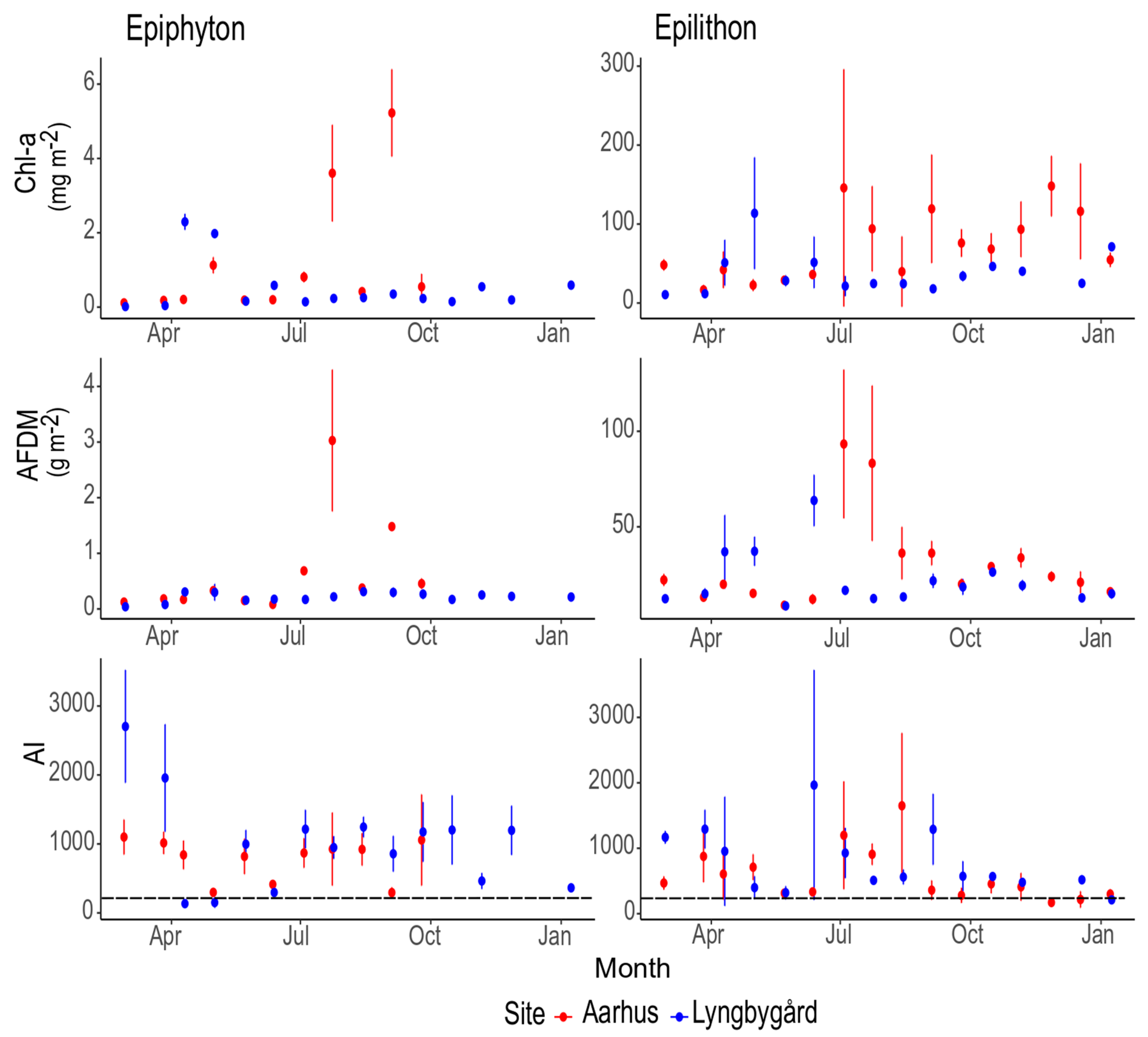
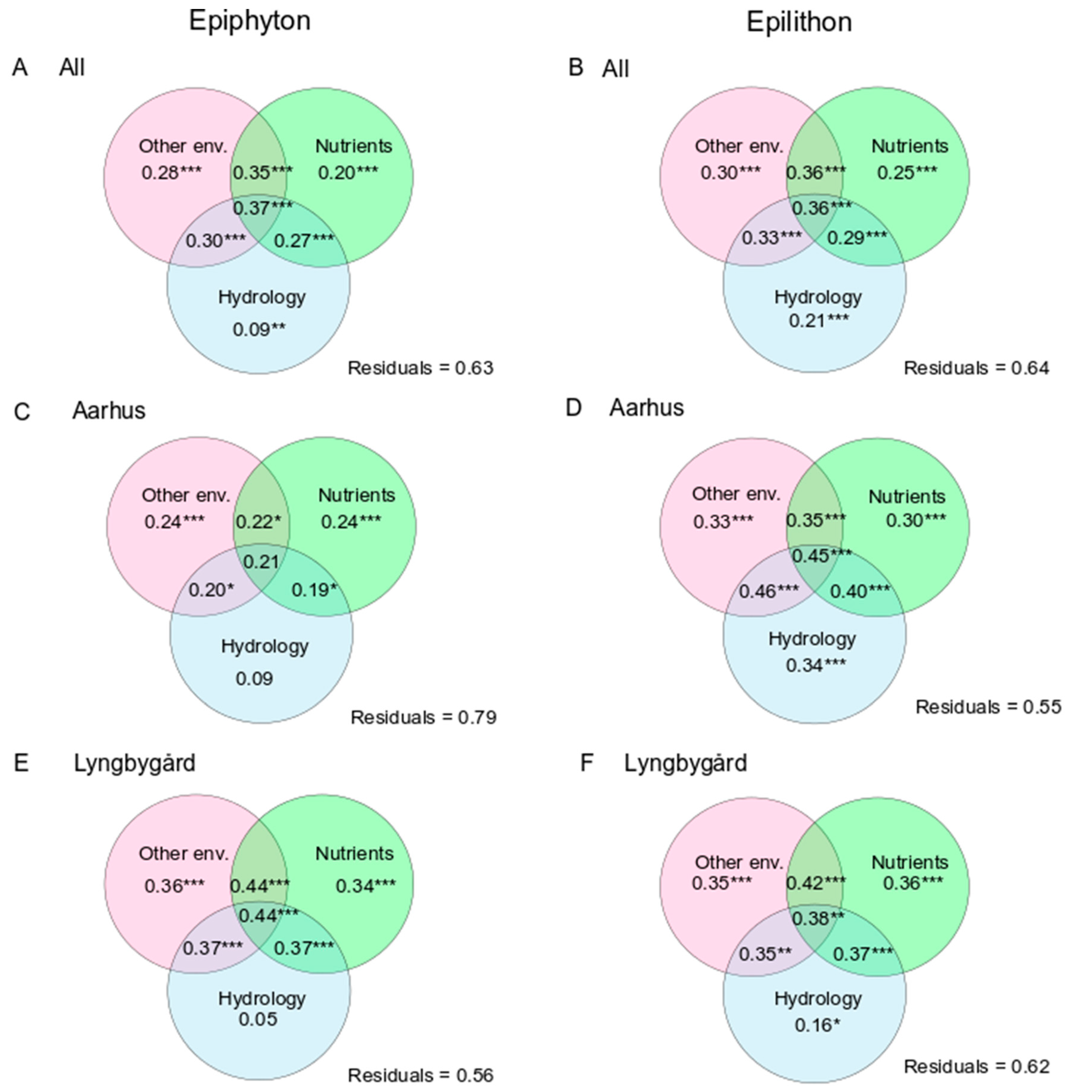
3.2. Biomass, AI and Main Drivers

The epiphyton and epilithon biomass (per substrate area) changed over the year in both streams (Figure 2). The concentrations of Chl-a (mean: 0.78 mg m−2, range: 0.02–5.22 mg m2) and AFDM (mean: 0.39 g m−2, range: 0.04–3.03 g m−2) in the epiphyton were much lower than in the epilithon (mean Chl-a: 55.55 mg m−2, range: 10.60–148.05 mg m−2 and mean AFDM: 26.27 g m−2, range: 8.60–93.33 g m−2). The AI of both biofilm types was generally higher than 200, indicating a high heterotrophic dominance (Figure 2), and AI was generally higher in the epiphyton (mean: 902, range: 134–2703) than in the epilithon (mean: 677, range: 177–1965). In both communities, AFDM peaked during the summer months (i.e., July), whereas the Chl-a of the epiphyton peaked twice, in spring (i.e., April) and in autumn (i.e., September).
When comparing epiphyton in the two streams, we found that Chl-a concentrations in Aarhus (1.15 mg m−2, range: 0.10–6.23 mg m−2) generally doubled the concentrations in Lyngbygård (0.52 mg m−2, range: 0.01–2.53 mg m−2). AFDM was also mostly higher in Aarhus (mean: 0.64 g m−2, range: 0.07–4.49 g m−2) than in Lyngbygård (mean: 0.21 g m−2, range: 0.03–0.47 g m−2), and AIs were 778 (range: 239–1787) and 993 (range: 103–3475), respectively. A similar pattern was observed for epilithon. The mean Chl-a concentrations in Aarhus doubled (71.87 mg m−2, range: 16.60–148.05 mg m−2) the concentrations in Lyngbygård (38.14 mg m−2, range: 10.60–113.66 mg m−2); AFDM was higher in Aarhus (mean: 30.28 g m−2; range: 8.95–93.33 g m−2) than in Lyngbygård (mean: 22.00 g m−2; range: 8.59–63.77 g m−2), and AIs in Aarhus and Lyngbygård streams were 677 (range: 171–1965) and 579 (range: 171–1649), respectively.
We found weak correlations between the environmental variables and the epiphytic and epilithic biomass and AI when analysing data from both streams together (Table S2). Only the epilithon Chl-a showed a significant and positive relationship with water PO43− concentration (Table 1). No significant models were obtained for epiphyton and epilithon biomass and AI when streams were analysed separately.

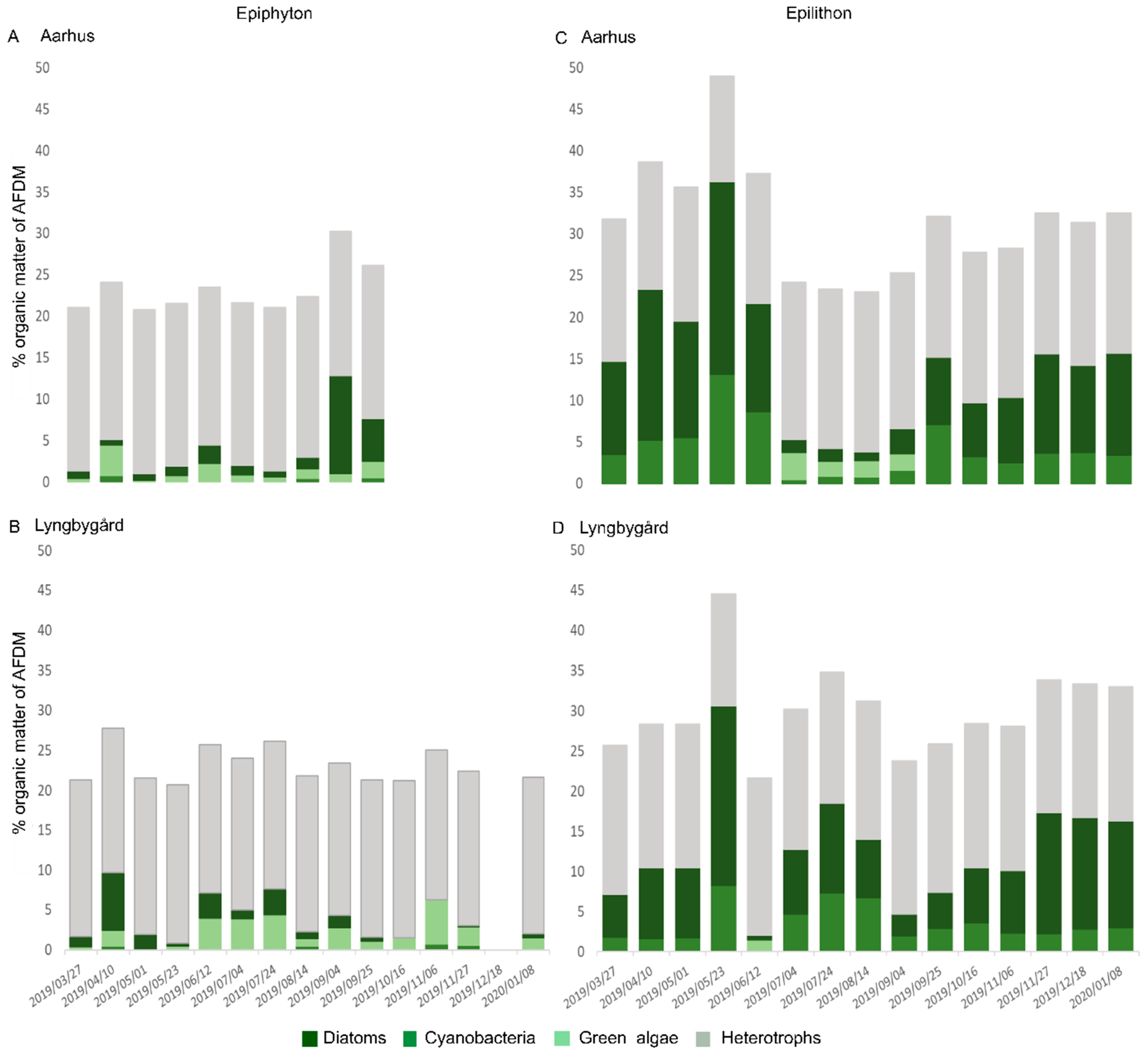
3.3. Algal Composition and Main Drivers

Over 50% of the epiphyton and epilithon consisted of dead organic matter and the algal composition changed throughout the year (Figure 3). As a general trend, the autotrophic community of epiphyton consisted of diatoms > green algae > cyanobacteria (very low), while the epilithon community consisted of diatoms > cyanobacteria > green algae. Peaks of diatoms in epiphyton were found in April at Lyngbygård and in September at Aarhus. Green algae were present in the epiphyton community throughout the year except for two peak times of the diatoms. In the epilithon community, the highest autotrophic community (diatoms and cyanobacteria) was observed in late May and the presence of green algae was only observed in summer in Aarhus stream.
Overall, DOC negatively correlated with epiphytic diatom biomass but positively correlated with epiphytic cyanobacteria biomass in Lyngbygård (Table 2). In epilithon, temperature negatively correlated with diatom biomass. Furthermore, epilithic green algae biomass positively linked with temperature and negatively correlated to DOC (Table 2). No significant models were obtained for epiphyton in Aarhus and epilithon in Lyngbygård.

3.4. Diatom Species Composition and Main Drivers

In total, 193 diatom species were found in our study, belonging to seven different families (i.e., Monoraphidees, Naviculacees, Araphidees, Centrophycidees, Surirellacees, Nitzschiacees and Brachyraphydees). We identified 135 species in epiphyton and 164 species in epilithon. The epiphyton diatom community was dominated by Cocconeis placentula var. euglypta Ehr. (25% in relative abundance), followed by Navicula lanceolate Ehr. (9%), Achnanthidium minutissimum Kütz. (7%), Navicula tripunctata (Müller) Bory (6%) and Gomphonema parvulum Kütz. (5%) (Table S3). The epilithon diatom community was dominated by Achnanthidium minutissimum (37% in relative abundance), followed by, Navicula lanceolate (10%), Cocconeis placentula var. euglypta (8%), Planothidium lanceolatum (Brébisson ex Kütz.) Lange-Bertalot (4%) and Planothidium frequentissimum Lange-Bertalot (3%) (Table S3).
A non-metric multidimensional scaling (NMDS) ordination of the biofilm diatom community composition revealed two distinct clusters (stress: 0.01, Figure 4A) suggesting that the diatom species composition of epiphyton and epilithon communities were significantly different from each other (Adonis, F = 7.08, p = 0.001). Additionally, the epiphyton and epilithon diatom community showed distinct separation according to stream (Figure 4B; stress: 0.16 and Adonis, F = 4.56, p = 0.001 and Figure 4D; stress: 0.14 and Adonis, F = 2.87, p = 0.008). Furthermore, the temporal dynamics of the epiphyton and epilithon diatom community showed greater variation in Lyngbygård compared to in Aarhus over the sampling year (Figure 4C,E). Epilithic diatom communities tended to come back to first sample completing a cyclic path while the epiphytic diatom communities had more distinctive start and end points.
According to the partial redundancy analysis (pRDA) the variation in the epiphytic diatom community can be explained by nutrients and other environmental factors (adj. R2 = 0.20 and 0.28, respectively, Figure 5A), with hydrology less important in both streams (Figure 5C,E). For epilithon, all three groups of variables were responsible for an equal amount of variation (adj. R2 = 0.30; 0.25, and 0.21), indicating that hydrology was more important for epilithon than for epiphyton (Figure 5B). The effect of hydrology on epilithon was especially pronounced in Aarhus (Figure 5D). The combination of any two and all three environmental variable categories better explained diatom-species composition in both communities than any individual categories, and the highest variability of the diatom community composition was explained by the shared contribution of all three categories in both epiphyton and epilithon, as 0.37 and 0.36 (adj. R2), respectively (Figure 5A,B).

4. Discussion

The results of the study revealed that the biofilm structural components, such as biomass, algal composition and diatom species composition were highly different for epiphyton and epilithon supporting H1. Further, some of our observations supported that epiphyton was less influenced by hydrological and nutrient regimes compared to epilithon (H2 and H3). The explanatory power using daily environmental measurements in a 3-week regime was lower than expected, but it was still within the range of previous studies.
The main structural differences between epiphyton and epilithon found in our study were that in epiphyton, unlike in epilithon, (1) the area-based biomass was about 50-fold lower, (2) the heterotrophic composition was higher, (3) the abundance of cyanobacteria was lower, and (4) the dominant diatom species were associated with low disturbance and high nutrient concentrations. In H1, we expected the biomass to be different between the two biofilms, which is shown in the results, but the expected difference was higher biomass in epiphyton than epilithon focusing on hydrological disturbances and nutrients solely. However, the results revealed an opposite trend. A higher biomass per substrate area for epilithon, compared with epiphyton have previously been found in river ecosystem [53] and lakes [54]. They emphasize that a higher epilithon biomass is most likely due higher stability [55,56] and the durability of gravel and stone substrates, whereas plant-decaying process and macrophyte allelopathic substances may lead to less biomass accrual on epiphyton [54]. Both biofilm communities showed a dominant heterotrophy similar to previous studies, e.g., [57,58]. However, we also found that epiphyton showed higher heterotrophy compared to epilithon, which suggests macrophytes to be a more favourable substrate for the heterotrophic community compared to the gravel/stone substrate [59].
Diatoms and green algae were the main algae communities in epiphyton, which is consistent with previous studies [22,60], and the presence of cyanobacteria was negligible. In contrast, cyanobacteria were more abundant than green algae in epilithon, particularly during summer months in Aarhus, where discharge and DIN concentrations were low. This is supported by Zlatanović, Fabian, Premke and Mutz [21] that noted a change in the epilithon community from diatoms to green algae and cyanobacteria under low flow periods. Diatom-composition was significantly different between epiphyton and epilithon in our study, which agrees with previous studies by Cantonati and Spitale [17] and Soininen and Eloranta [55]. In contrast, Winter and Duthie [25] concluded that the diatom community structure of the two communities is not consistently different in streams surrounded by mixed-land use such as urban, agriculture and woodlands. Furthermore, the dominant epiphyton diatom species found was Cocconeis placentula var. euglypta whereas Achnanthidium minutissimum dominated in epilithon diatom community, which follows the findings in [23,55,56].
Differences in the dominant diatom species in epiphyton and epilithon support hypotheses H2 and H3 stating that epilithon is more strongly related to hydrology and nutrient concentrations in streams than epiphyton. The dominating species in epilithon, Achnanthidium minutissimum, is well-known as a species adapted to a high velocity environment [61], whereas the species that were found in high abundances in the epiphyton community are often found in a high nutrient environment under agricultural influence (e.g., Gomphonema spp. and Encyonema sp., Table S3) [62]. Therefore, differences in species composition of the epiphyton and epilithon support that the epilithon is more dependent on the water-nutrient concentration and hydraulic disturbances, validating the H2 and H3 hypotheses. This was further supported by the fact that the temporal trajectories of diatom community compositions showed the epilithon community completing a cyclic path, moving back to its original state at the end of year while the epiphyton start and end points were different. Closer associations of the epiphytic community with macrophyte characteristics and the life cycle were found than with environmental factors, which may cause the high turnover rate of the species and the lower persistence of communities compared to epilithon as reported by [55] and the discontinuity of the cyclic path found in our study, despite the reoccurrence of environmental conditions [63,64].
We also found direct support for H3 in the multiple regression analyses. We found that the epilithic biomass (Chl-a) was better related to nutrients than epiphyton (Table 1). Epilithic Chl-a demonstrated positive association with PO43− and a similar relationship was found in many previous studies [65,66]. Further, H2 and H3 were directly confirmed by the results of the pRDA analyses, showing variation of the epilithic diatom species’ composition, more associated with hydrology and nutrients than epiphyton (Figure 5). The influence of hydrology (i.e., discharge, current velocity, low flow, high flow) on the epilithon structure was highly recognized in many previous studies in lotic systems [6,67,68,69] and nutrients were identified as an important factor in driving epilithic diatom composition [28,55]. Furthermore, the low association of epiphyton with water nutrient concentrations supports the suggestion that the epiphyton community may depend on nutrients released from the macrophyte [13,59]. Our results support results from Gosselain et al. [70] highlighting that epiphyton was related to physical variables such as light, macrophyte architecture and hydrology (i.e., seasonal water level variations) in the order of decreasing importance.
Overall, we observed considerable differences in the biofilm structural components between the two study streams, and these differences were predominantly driven by differences in light availability, DOC and PO43− (Figure 1). For example, the biofilm biomass was twice as high in Aarhus compared to Lyngbygård, due to higher light availability caused by lower riparian vegetation cover and higher PO43− concentrations in Aarhus. High biofilm Chl-a in Lyngbygård was observed only in spring under low riparian shading prior to leaf out, where it had maximum light availability due to low shading by spring riparian vegetation [71]. In Aarhus, we observed a higher abundance of Cladophora sp. (filamentous green algae) during summer months, and the eutrophic indicator species Achnanthidium minutissimum showed high abundance (relative abundance doubled in epilithon and four times higher in epiphyton) at high PO43− concentration compared to Lyngbygård [62]. Thus, although the two study streams showed similar land use and catchment size, local differences driven by light, DOC and PO43− were important to site-specific biofilm structure.
The explanatory power of the environmental factors on the epiphytic and epilithic structural responses was overall low across the two streams (36–37%), and lower in Aarhus (21–45%) than in Lyngbygård (38–44%). Usually, nutrient concentrations are only measured once or a few times during biofilm accrual, and by using daily measurements we expected a higher explanatory power. However, the explanatory power was not significantly different from earlier studies such as [72], in which the authors found that 44–49% of variation in mean monthly biofilm Chl-a was explained by hydrology and nutrient concentration in New Zealand streams. Another study by Lévesque et al. [73] found that environmental variables were only able to explain 15.4% of the variation of epiphyton biomass in a fluvial system in Canada. Part of the general high and unexplained variation models on epiphytic and epilithic biomass, could result from the fact that (i) reach-scale variables do not reflect micro-scale variables as strongly as expected from previous studies [5,29,30], and that biofilms thus may be more closely linked to the micro-habitat mediated environmental variables than the reach-scale measurements [74]. Furthermore, (ii) biofilms constitute complex communities where individual components respond differently to environmental variables, e.g., DOC acts as a nutrient for the heterotrophic community but high DOC may lead to limited light availability for autotrophs and for their photosynthesis [73,75]. In addition, (iii) biofilm community compartments are highly interactive; for example, autotrophic communities in the biofilm may use CO2 for their primary production, derived from the respiration of the heterotrophic community internally [16]. Moreover, (iv) interactions between biofilms and their substrate such as epiphytic biofilm and host macrophytes may also show competitive and mutualistic relationships for nutrients, which may be more important than the nutrient concentrations in the surrounding flowing water [14]. In order to improve the predictive strength of models on epiphytic and epilithic biofilm, measurements of environmental variables at the micro-habitat scale may be required, or more sensitive data analyses, such as a time series analysis as in [76].

5. Conclusions

Epiphyton and epilithon showed distinct structural differences during a year in two agricultural streams in terms of biomass, algal composition, and diatom species composition. Epiphyton structural properties were less affected by hydrological regimes and water nutrient concentrations than epilithon, indicating that epilithon is more dependent on external water nutrients to fulfil nutrient requirements, while epiphyton can take advantage of macrophyte leachates. Other environmental variables such as light, temperature and DOC played an important role in driving epiphyton and epilithon structural differences between the two streams. We observed a generally low explanatory power of the included environmental variables on the biofilm structure even though we used daily measurements. Future studies should address the interactions within biofilm communities, interactions with their substrates and interactions with other biota to better understand the underlying controlling mechanisms of the epiphyton and epilithon structure in agricultural streams. Using micro-scale measurements instead of reach-scale measurements may further enhance the understanding of environmental drivers of the epiphytic and epilithic community structure.

Supplementary Materials

The following are available online at https://www.mdpi.com/article/10.3390/w13233443/s1, Figure S1: Location of monitored two agricultural streams at Aarhus, Denmark, study sites and studied stream algae communities. Figure S2: Correlations between environmental variables, Table S1: Description of nine environmental variables used in our study, Table S2: Epiphyton and epilithon biomass and AI related to environmental variables, Table S3: Relative abundance (%) of 20 most abundant diatom species in the biofilms

Author Contributions

Conceptualization: L.W., N.W., N.F. and T.R.; Data curation: L.W., P.G.-G. and C.H.; Formal analysis: L.W., P.G.-G., C.H. and T.R.; Funding acquisition: A.B.-P. and T.R.; Supervision: N.W., N.F. and T.R.; Writing—original draft: L.W.; Writing—review and editing: L.W., N.W., P.G.-G., N.F., A.B.-P. and T.R. All authors have read and agreed to the published version of the manuscript.

Funding

This research was funded by Velux Foundation, Denmark (grant #22933 for T.R.). During this work, L.W. received funding from the German Academic Exchange Service (DAAD) (No. 91690872). We acknowledge financial support for APC by Land Schleswig-Holstein within the funding program Open Access Publikationsfonds.

Institutional Review Board Statement

Not applicable.

Informed Consent Statement

Not applicable.

Acknowledgments

We thank laboratory crew at Department of Biology, Aarhus University, Denmark for their immense help in conducting experiments and laboratory analyses. We are grateful to editor and two anonymous reviewers for their constructive feedback on initial draft.

Conflicts of Interest

The authors declare that they have no known competing financial interests or personal relationships that could have appeared to influence the work reported in this paper.

References

  1. Battin, T.J.; Kaplan, L.A.; Newbold, J.D.; Hansen, C.M. Contributions of microbial biofilms to ecosystem processes in stream mesocosms. Nature 2003, 426, 439–442. [Google Scholar] [CrossRef]
  2. Besemer, K.; Peter, H.; Logue, J.B.; Langenheder, S.; Lindström, E.S.; Tranvik, L.J.; Battin, T.J. Unraveling assembly of stream biofilm communities. ISME J. 2012, 6, 1459–1468. [Google Scholar] [CrossRef] [PubMed] [Green Version]
  3. Romaní, A.M. Freshwater Biofilms. In Biofouling; Wiley-Blackwell: Oxford, UK, 2009; pp. 137–153. [Google Scholar]
  4. Biggs, B.J.; Thomsen, H.A. Disturbance of stream periphyton by perturbations in shear stress: Time to structural failure and differences in community resistance. J. Phycol. 1995, 31, 233–241. [Google Scholar] [CrossRef]
  5. Biggs, B.J. Hydraulic habitat of plants in streams. Regul. Rivers Res. Manag. 1996, 12, 131–144. [Google Scholar] [CrossRef]
  6. Guo, K.; Wu, N.; Manolaki, P.; Baattrup-Pedersen, A.; Riis, T. Short-period hydrological regimes outperform physicochemical variables in shaping stream diatom traits and biofilm community functions. Sci. Total Environ. 2020, 743, 140720. [Google Scholar] [CrossRef]
  7. Wu, N.; Thodsen, H.; Andersen, H.E.; Tornbjerg, H.; Baattrup-Pedersen, A.; Riis, T. Flow regimes filter species traits of benthic diatom communities and modify the functional features of lowland streams-a nationwide scale study. Sci. Total Environ. 2019, 651, 357–366. [Google Scholar] [CrossRef]
  8. Alnoee, A.B.; Riis, T.; Baattrup-Pedersen, A. Comparison of metabolic rates among macrophyte and nonmacrophyte habitats in streams. Freshw. Sci. 2016, 35, 834–844. [Google Scholar] [CrossRef] [Green Version]
  9. Levi, P.S.; Riis, T.; Alnøe, A.B.; Peipoch, M.; Maetzke, K.; Bruus, C.; Baattrup-Pedersen, A. Macrophyte complexity controls nutrient uptake in lowland streams. Ecosystems 2015, 18, 914–931. [Google Scholar] [CrossRef]
  10. Demarty, M.; Prairie, Y.T. In situ dissolved organic carbon (DOC) release by submerged macrophyte–epiphyte communities in southern Quebec lakes. Can. J. Fish. Aquat. Sci. 2009, 66, 1522–1531. [Google Scholar] [CrossRef]
  11. Zhai, X.; Piwpuan, N.; Arias, C.A.; Headley, T.; Brix, H. Can root exudates from emergent wetland plants fuel denitrification in subsurface flow constructed wetland systems? Ecol. Eng. 2013, 61, 555–563. [Google Scholar] [CrossRef]
  12. Burkholder, J.M.; Wetzel, R.G. Epiphytic alkaline phosphatase on natural and artificial plants in an oligotrophic lake: Re-evaluation of the role of macrophytes as a phosphorus source for epiphytes. Limnol. Oceanogr. 1990, 35, 736–747. [Google Scholar] [CrossRef]
  13. Bojorge-García, M.; Carmona, J.; Ramírez, R. Species richness and diversity of benthic diatom communities in tropical mountain streams of Mexico. Inland Waters 2014, 4, 279–292. [Google Scholar] [CrossRef] [Green Version]
  14. Wijewardene, L.; Wu, N.; Fohrer, N.; Riis, T. Epiphytic biofilms in freshwater and interactions with macrophytes: Current understanding and future directions. Aquat. Bot. 2022, 176, 103467. [Google Scholar] [CrossRef]
  15. Brodersen, K.E.; Koren, K.; Revsbech, N.P.; Kühl, M. Strong leaf surface basification and CO2 limitation of seagrass induced by epiphytic biofilm microenvironments. Plant Cell Environ. 2020, 43, 174–187. [Google Scholar] [CrossRef] [PubMed]
  16. Allen, H.L. Primary productivity, chemo-organotrophy, and nutritional interactions of epiphytic algae and bacteria on macrophytes in the littoral of a lake. Ecol. Monogr. 1971, 41, 97–127. [Google Scholar] [CrossRef]
  17. Cantonati, M.; Spitale, D. The role of environmental variables in structuring epiphytic and epilithic diatom assemblages in springs and streams of the Dolomiti Bellunesi National Park (south-eastern Alps). Fundam. Appl. Limnol. Arch. Für Hydrobiol. 2009, 174, 117–133. [Google Scholar] [CrossRef]
  18. Roberts, B.J.; Mulholland, P.J.; Hill, W.R. Multiple Scales of Temporal Variability in Ecosystem Metabolism Rates: Results from 2 Years of Continuous Monitoring in a Forested Headwater Stream. Ecosystems 2007, 10, 588–606. [Google Scholar] [CrossRef]
  19. Lowe, R.L.; LaLiberte, G.D. Benthic stream algae: Distribution and structure. In Methods in Stream Ecology; Elsevier: Amsterdam, The Netherlands, 2017; Volume 1, pp. 193–221. [Google Scholar]
  20. Tang, T.; Cai, Q.; Liu, R.; Li, D.; Xie, Z. Distribution of epilithic algae in the Xiangxi River system and their relationships with environmental factors. J. Freshw. Ecol. 2002, 17, 345–352. [Google Scholar] [CrossRef]
  21. Zlatanović, S.; Fabian, J.; Premke, K.; Mutz, M. Shading and sediment structure effects on stream metabolism resistance and resilience to infrequent droughts. Sci. Total Environ. 2018, 621, 1233–1242. [Google Scholar] [CrossRef] [PubMed]
  22. Costică, M.; Costică, N.; Stratu, A. Contributions to the Knowledge of Aquatic and Paludous Macrophytes and of Some Epiphytic Algae with Role in Processes of Self-Cleaning in the Urban Sector of Nicolina River-Iasi. Present Environ. Sustain. Dev. 2018, 12, 61–72. [Google Scholar] [CrossRef] [Green Version]
  23. Shamsudin, L.; Sleigh, M.A. Seasonal changes in composition and biomass of epiphytic algae on the macrophyte Ranunculus penicillatus in a chalk stream, with estimates of production, and observations on the epiphytes of Cladophora glomerata. Hydrobiologia 1995, 306, 85–95. [Google Scholar] [CrossRef]
  24. Xia, P.; Yan, D.; Sun, R.; Song, X.; Lin, T.; Yi, Y. Community composition and correlations between bacteria and algae within epiphytic biofilms on submerged macrophytes in a plateau lake, southwest China. Sci. Total Environ. 2020, 727, 138398. [Google Scholar] [CrossRef]
  25. Winter, J.G.; Duthie, H.C. Stream epilithic, epipelic and epiphytic diatoms: Habitat fidelity and use in biomonitoring. Aquat. Ecol. 2000, 34, 345–353. [Google Scholar] [CrossRef]
  26. Soininen, J. Environmental and spatial control of freshwater diatoms—A review. Diatom Res. 2007, 22, 473–490. [Google Scholar] [CrossRef]
  27. Yang, Y.; Cao, J.-X.; Pei, G.-F.; Liu, G.-X. Using benthic diatom assemblages to assess human impacts on streams across a rural to urban gradient. Environ. Sci. Pollut. Res. 2015, 22, 18093–18106. [Google Scholar] [CrossRef] [PubMed]
  28. Munn, M.D.; Waite, I.; Konrad, C.P. Assessing the influence of multiple stressors on stream diatom metrics in the upper Midwest, USA. Ecol. Indic. 2018, 85, 1239–1248. [Google Scholar] [CrossRef]
  29. Biggs, B.J.F.; Stevenson, R.J.; Lowe, R.L. A habitat matrix conceptual model for stream periphyton. Arch. Fur Hydrobiol. 1998, 143, 21–56. [Google Scholar] [CrossRef]
  30. Biggs, B.J.F.; Nikora, V.I.; Snelder, T.H. Linking scales of flow variability to lotic ecosystem structure and function. River Res. Appl. 2005, 21, 283–298. [Google Scholar] [CrossRef]
  31. Riis, T. Dispersal and colonisation of plants in lowland streams: Success rates and bottlenecks. Hydrobiologia 2008, 596, 341–351. [Google Scholar] [CrossRef]
  32. Thimijan, R.W.; Heins, R.D. Photometric, radiometric, and quantum light units of measure: A review of procedures for interconversion. HortScience 1983, 18, 818–822. [Google Scholar]
  33. Steinman, A.D.; Lamberti, G.A.; Leavitt, P.R.; Uzarski, D.G. Biomass and pigments of benthic algae. In Methods in Stream Ecology; Elsevier: Amsterdam, The Netherlands, 2017; Volume 1, pp. 223–241. [Google Scholar]
  34. Lakatos, G. Composition of reed periphyton (biotecton) in the Hungarian part of lake Fertö. BFB-Bericht 1989, 71, 125–134. [Google Scholar]
  35. Li, H.-P.; Gong, G.-C.; Hsiung, T.-M. Phytoplankton pigment analysis by HPLC and its application in algal community investigations. Bot. Bull. Acad. Sin. 2002, 43, 283–290. [Google Scholar]
  36. Kahlert, M.; McKie, B.G. Comparing new and conventional methods to estimate benthic algal biomass and composition in freshwaters. Environ. Sci. Process. Impacts 2014, 16, 2627–2634. [Google Scholar] [CrossRef] [PubMed]
  37. Garrido, M.; Cecchi, P.; Malet, N.; Bec, B.; Torre, F.; Pasqualini, V. Evaluation of FluoroProbe® performance for the phytoplankton-based assessment of the ecological status of Mediterranean coastal lagoons. Environ. Monit. Assess. 2019, 191, 204. [Google Scholar] [CrossRef]
  38. Rosero-López, D.; Walter, M.T.; Flecker, A.S.; Ontaneda, D.F.; Dangles, O. Standardization of instantaneous fluoroprobe measurements of benthic algal biomass and composition in streams. Ecol. Indic. 2021, 121, 107185. [Google Scholar] [CrossRef]
  39. Sanzone, D.M.; Tank, J.L.; Meyer, J.L.; Mulholland, P.J.; Findlay, S.E. Microbial incorporation of nitrogen in stream detritus. Hydrobiologia 2001, 464, 27–35. [Google Scholar] [CrossRef]
  40. Bey, M.; Ector, L. Atlas des Diatrs d’eau de la Région Rhône-Alpes. 2013, pp. 1–1182. Available online: http://www.auvergne-rhone-alpes.developpement-durable.gouv.fr/atlas-des-diatomees-a3480.html (accessed on 10 October 2021).
  41. Hofmann, G.; Werum, M.; Lange-Bertalot, H. Diatomeen im Süßwasser-Benthos von Mitteleuropa: Bestimmungsflora Kieselalgen für die ökologische Praxis; über 700 der häufigsten Arten und ihrer Ökologie; Gantner: Ruggell, Liechtenstein, 2011. [Google Scholar]
  42. Cantonati, M.; Kelly, M.G.; Lange-Bertalot, H. Freshwater Benthic Diatoms of Central Europe: Over 800 Common Species Used in Ecological Assessment; Koeltz Botanical Books: Oberreifenberg, Germany, 2017; pp. 1–942. [Google Scholar]
  43. Bąk, M.; Witkowski, A.; Żelazna-Wieczorek, J.; Wojtal, A.; Szczepocka, E.; Szulc, K.; Szulc, B. Klucz do Oznaczania Okrzemek w Fitobentosie na Potrzeby Oceny Stanu Ekologicznego wód Powierzchniowych w Polsce; Biblioteka Monitoringu Srodowiska: Warszawa, Poland, 2012. [Google Scholar]
  44. R Core Team. R Software: Version 4.0.2; R Foundation for Statistical Computing: Vienna, Austria, 2020. [Google Scholar]
  45. Wickham, H. ggplot2: Elegant Graphics for DATA Analysis; Springer: Berlin/Heidelberg, Germany, 2016. [Google Scholar]
  46. Wei, T.; Simko, V. R Package “corrplot”: Visualization of a Correlation Matrix (Version 0.84). 2017. Available online: https://github.com/taiyun/corrplot (accessed on 10 October 2021).
  47. Oksanen, J.; Blanchet, F.; Friendly, M.; Kindt, R.; Legendre, P.; Mcglinn, D.; Stevens, M. Package—Vegan: Community Ecology Package. R Package Version 2.5-6. 2020. Available online: https://github.com/vegandevs/vegan (accessed on 10 October 2021).
  48. De Caceres, M. Package ‘Vegclust’. 2010. Available online: https://emf-creaf.github.io/vegclust (accessed on 10 October 2021).
  49. Lepš, J.; Šmilauer, P. Multivariate Analysis of Ecological Data Using CANOCO; Cambridge University Press: Cambridge, UK, 2003. [Google Scholar]
  50. Cornejo, A.; Tonin, A.M.; Checa, B.; Tuñon, A.R.; Pérez, D.; Coronado, E.; González, S.; Ríos, T.; Macchi, P.; Correa-Araneda, F.; et al. Effects of multiple stressors associated with agriculture on stream macroinvertebrate communities in a tropical catchment. PLoS ONE 2019, 14, e0220528. [Google Scholar] [CrossRef] [Green Version]
  51. Inkscape Project. Inkscape; Prentice hall press: Hoboken, NJ, USA, 2020. [Google Scholar]
  52. Ripley, B.; Venables, B.; Bates, D.M.; Hornik, K.; Gebhardt, A.; Firth, D.; Ripley, M.B. Package ‘mass’. Cran R 2013, 538, 113–120. [Google Scholar]
  53. Belyaeva, P. Photosynthetic pigments of phytoperiphyton in the Sylva River (Middle Ural). Inland Water Biol. 2017, 10, 52–58. [Google Scholar] [CrossRef]
  54. Kahlert, M.; Pettersson, K. The impact of substrate and lake trophy on the biomass and nutrient status of benthic algae. Hydrobiologia 2002, 489, 161–169. [Google Scholar] [CrossRef]
  55. Soininen, J.; Eloranta, P. Seasonal persistence and stability of diatom communities in rivers: Are there habitat specific differences? Eur. J. Phycol. 2004, 39, 153–160. [Google Scholar] [CrossRef]
  56. Zelnik, I.; Sušin, T. Epilithic Diatom Community Shows a Higher Vulnerability of the River Sava to Pollution during the Winter. Diversity 2020, 12, 465. [Google Scholar] [CrossRef]
  57. Fernandes, V.; Esteves, F. The use of indices for evaluating the periphytic community in two kinds of substrate in Imboassica Lagoon, Rio de Janeiro, Brazil. Braz. J. Biol. 2003, 63, 233–243. [Google Scholar] [CrossRef] [PubMed]
  58. Lock, M.A.; Wallace, R.R.; Costerton, J.W.; Ventullo, R.M.; Charlton, S.E. River Epilithon: Toward a Structural-Functional Model. Oikos 1984, 42, 10–22. [Google Scholar] [CrossRef]
  59. Wolters, J.-W.; Reitsema, R.E.; Verdonschot, R.C.M.; Schoelynck, J.; Verdonschot, P.F.M.; Meire, P. Macrophyte-specific effects on epiphyton quality and quantity and resulting effects on grazing macroinvertebrates. Freshw. Biol. 2019, 64, 1131–1142. [Google Scholar] [CrossRef]
  60. Piirsoo, K.; Vilbaste, S.; Truu, J.; Pall, P.; Trei, T.; Tuvikene, A.; Viik, M. Origin of phytoplankton and the environmental factors governing the structure of microalgal communities in lowland streams. Aquat. Ecol. 2007, 41, 183–194. [Google Scholar] [CrossRef]
  61. Shen, R.; Ren, H.; Yu, P.; You, Q.; Pang, W.; Wang, Q. Benthic Diatoms of the Ying River (Huaihe River Basin, China) and Their Application in Water Trophic Status Assessment. Water 2018, 10, 1013. [Google Scholar] [CrossRef] [Green Version]
  62. Lu, X.; Liu, Y.; Fan, Y. Diatom Taxonomic Composition as a Biological Indicator of the Ecological Health and Status of a River Basin under Agricultural Influence. Water 2020, 12, 2067. [Google Scholar] [CrossRef]
  63. Ferreiro, N.; Giorgi, A.; Feijoó, C. Effects of macrophyte architecture and leaf shape complexity on structural parameters of the epiphytic algal community in a Pampean stream. Aquat. Ecol. 2013, 47, 389–401. [Google Scholar] [CrossRef]
  64. Pettit, N.E.; Ward, D.P.; Adame, M.F.; Valdez, D.; Bunn, S.E. Influence of aquatic plant architecture on epiphyte biomass on a tropical river floodplain. Aquat. Bot. 2016, 129, 35–43. [Google Scholar] [CrossRef] [Green Version]
  65. Bowden, W.B.; Peterson, B.J.; Finlay, J.C.; Tucker, J. Epilithic chlorophyll a, photosynthesis, and respiration in control and fertilized reaches of a tundra stream. Hydrobiologia 1992, 240, 121–131. [Google Scholar] [CrossRef]
  66. Hill, W.R.; Fanta, S.E.; Roberts, B.J. Quantifying phosphorus and light effects in stream algae. Limnol. Oceanogr. 2009, 54, 368–380. [Google Scholar] [CrossRef] [Green Version]
  67. Ács, É.; Kiss, K.T. Effects of the water discharge on periphyton abundance and diversity in a large river (River Danube, Hungary). Hydrobiologia 1993, 249, 125–133. [Google Scholar] [CrossRef]
  68. Matthaei, C.D.; Piggott, J.J.; Townsend, C.R. Multiple stressors in agricultural streams: Interactions among sediment addition, nutrient enrichment and water abstraction. J. Appl. Ecol. 2010, 47, 639–649. [Google Scholar] [CrossRef]
  69. Moulton, T.P.; Souza, M.L.; Walter, T.L.; Krsulovic, F.A.M. Patterns of periphyton chlorophyll and dry mass in a neotropical stream: A cheap and rapid analysis using a hand-held fluorometer. Mar. Freshw. Res. 2009, 60, 224–233. [Google Scholar] [CrossRef]
  70. Gosselain, V.; Hudon, C.; Cattaneo, A.; Gagnon, P.; Planas, D.; Rochefort, D. Physical variables driving epiphytic algal biomass in a dense macrophyte bed of the St. Lawrence River (Quebec, Canada). Hydrobiologia 2005, 534, 11–22. [Google Scholar] [CrossRef]
  71. Tank, J.L.; Martí, E.; Riis, T.; von Schiller, D.; Reisinger, A.J.; Dodds, W.K.; Whiles, M.R.; Ashkenas, L.R.; Bowden, W.B.; Collins, S.M.; et al. Partitioning assimilatory nitrogen uptake in streams: An analysis of stable isotope tracer additions across continents. Ecol. Monogr. 2018, 88, 120–138. [Google Scholar] [CrossRef] [Green Version]
  72. Biggs, B.J.F. Eutrophication of streams and rivers: Dissolved nutrient-chlorophyll relationships for benthic algae. J. N. Am. Benthol. Soc. 2000, 19, 17–31. [Google Scholar] [CrossRef] [Green Version]
  73. Lévesque, D.; Hudon, C.; James, P.M.A.; Legendre, P. Environmental factors structuring benthic primary producers at different spatial scales in the St. Lawrence River (Canada). Aquat. Sci. 2017, 79, 345–356. [Google Scholar] [CrossRef]
  74. Morin, J.O.n.; Kimball, K.D. Relationship of macrophyte-mediated changes in the water column to periphyton composition and abundance. Freshw. Biol. 1983, 13, 403–414. [Google Scholar] [CrossRef]
  75. Sobczak, W.V.; Findlay, S. Variation in Bioavailability of Dissolved Organic Carbon among Stream Hyporheic Flowpaths. Ecology 2002, 83, 3194–3209. [Google Scholar] [CrossRef]
  76. Lange, H. Time-Series Analysis in Ecology. In eLS; Wiley-VCH GmbH: Weinheim, Germany, 2006. [Google Scholar]
Figure 1. Changes in environmental variables over the study period. Description of calculations of these variables can be found in Table S1. All environmental data derived from measurements obtained in the period of 21 days before the sampling date: (A): cumulative light (Photons m−2 day−1); (B): mean temperature (°C); (C): mean DOC (mg L−1); (D): median discharge (Qmed, L s−1); (E): coefficient of variation of discharge (CV of Q, %); (F): frequency of low flow (FreLow, days); (G): frequency of high flow (FreHigh, days); (H): mean PO43− concentration (mg L−1) in water and (I): mean DIN concentration (mg L−1) in water.
Water 13 03443 g001
Figure 2. Changes in epiphytic and epilithic biomass and AI (per substrate area) throughout the annual study of the two streams. Dots and error bars denote mean and standard deviation values, respectively (n = 3). The horizontal dashed lines in AI graphs show the index value of 200, which mark the limit between heterotrophic (above) or autotrophic (below) predominance in the biofilms.
Water 13 03443 g002
Figure 3. Changes of biofilm composition over the year. (A): epiphyton at Aarhus stream; (B): epiphyton at Lyngbygård stream; (C): epilithon at Aarhus stream and (D): epilithon at Lyngbygård stream. Epiphyton only present at samplings date where macrophytes are present.
Water 13 03443 g003
Figure 4. Differences in diatom species composition and trajectories of community change over the study year. (A): epiphyton and epilithon diatom species composition; (B): epiphytic diatom communities in two streams; (C): trajectories of epiphytic community change over the study year; (D): epilithic diatom communities in two streams and (E): trajectories of epilithic community change over the year.
Water 13 03443 g004
Figure 5. Partial redundancy analysis (pRDA) for quantifying the variation of diatom community composition explained by hydrology (Qmed, CV of Q), nutrients (PO43−, DIN) and other environmental variables (other env: light, temperature, DOC), their shared contribution and unexplained variance (i.e., Residual). Each subplot represents the studied diatom assemblages as (A): epiphyton; (B): epilithon; (C): epiphyton in Aarhus stream; (D): epilithon in Aarhus stream; (E): epiphyton in Lyngbygård stream and (F): epilithon in Lyngbygård stream. Significance codes: * p < 0.05, ** p < 0.01, *** p < 0.001. All environmental data derived from measurements taken in the period of 21 days before sampling date (Figure 1).
Water 13 03443 g005
Table 1. Multiple regression models on biomass and AI of epiphyton and epilithon (p < 0.05 and lowest AIC) for all data from the two study streams. Significant variables in the models are shown in bold. All environmental data derived from measurements were taken in the period of 21 days before sampling date (Figure 1).
ModelResponse
Variables
Environmental VariablesEstimatep ValueModel adj.R2Model
Significance
AIC
EpiphytonChl-aNo significant model
AFDMTemperature0.3060.1120.2180.02372.215
DOC−0.3520.069
AINo significant model
EpilithonChl-aCV of Q−0.2590.1280.2240.0187.531
PO43−0.3860.027
AFDMNo significant model
AICV of Q0.2980.0930.1640.02989.946
PO43−−0.2820.111
Table 2. Multiple regression models on algal composition in epiphyton and epilithon (p < 0.05 and lowest AIC). Significant variables in the models are shown in bold. All environmental data derived from measurements taken in the period of 21 days before sampling date (Figure 1).
ModelResponse
Variables
Environmental VariablesEstimatep ValueModel adj.R2Model
Significance
AIC
EpiphytonDiatomDOC−0.5020.0120.2180.01266.106
Cyanobacteria Qmed0.3490.0870.2170.0367.048
CV of Q0.3090.127
Green algaeNo significant model
EpilithonDiatomTemperature−0.5620.0010.2910.00178.752
CyanobacteriaNo significant model
Green algaeTemperature0.6240.0280.3650.00277.231
DOC−0.5960.006
Qmed0.4600.161
Epiphyton—LyngbygårdDiatomLight0.3900.1470.3880.02737.480
DOC−0.4130.127
CyanobacteriaDOC0.5700.0330.2690.033 39.183
Green algaeNo significant model
Epilithon—AarhusDiatomTemperature−0.6790.0050.4190.00538.270
CyanobacteriaNo significant model
Green algaeTemperature0.3530.1790.5430.00435.466
DOC−0.4950.069
Publisher’s Note: MDPI stays neutral with regard to jurisdictional claims in published maps and institutional affiliations.

