Abstract
With the depletion of fossil energy sources, clean energy has become a growing concern for scholars. Vortex-Induced Vibration Aquatic Clean Energy (VIVACE), a device that uses water flow energy to generate electricity, has attracted much attention for its broad applicability and other advantages. Particle Image Velocimetry (PIV) experiments were conducted to improve the efficiency of the VIVACE device in low-velocity areas. The present study investigated the effects of the Blockage ratio (Br), Reynolds number (Re = ρU0D/μ), and Aspect ratio (Ar = B/D, width-to-height) of rectangular cylinders on flow characteristics. The influence of the Ar, Br, and Re on the flow field structure was systematically analyzed in terms of the time-averaged flow field, Reynolds shear stress, space–time correlation, vorticity field, and water pressure characteristics. The vorticity field was deconstructed by Proper Orthogonal Decomposition (POD). The results show that the first two orders of POD modal energy accounted for 75% of the total energy, indicating that the first two modes can be used to identify the large-scale vortex structure. The main water pressure frequency and vortex shedding frequency (f) had a high degree of consistency. Thus, vortex shedding was the main cause of wall water pressure fluctuations. Given the blockage effect, the shear layer’s development spanwise was restricted. Moreover, the blockage effect increased the local flow velocity and accelerated the vortex shedding. The dimensionless time-averaged flow velocity U/U0 increased to 1.5, and the frequency of vortex shedding increased by approximately 25% when the Br increased from 0.067 to 0.25. The frequency increased by 25% when the Ar decreased from 0.5 to 0.2. The experimental results also provide a new idea for optimizing the VIVACE device.
1. Introduction
Flow around a blunt body has numerous technical applications, such as air ventilation, urban structures, and hydraulic engineering [1,2,3]. When fluid flows through an obtuse body to create vortex shedding, the structure absorbs most of the fluid’s kinetic energy, resulting in a certain degree of obtuse body vibration called fluid-induced vibration (FIV) [4,5,6]. FIV is a double-edged sword. On the one hand, it damages buildings such as bridges and gates. On the other hand, FIV can also be utilized for power generation, as in the VIVACE device invented by Bernitsas and patented through the University of Michigan [7]. The VIVACE converter uses vortex-induced vibration (VIV) to generate energy successfully and with a high power conversion ratio from a fluid flow. The VIVACE device offers the following major benefits over turbine and wave energy generation: (1) a more comprehensive range of applications; (2) completely clean and renewable energy; (3) low-risk equipment in the energy acquisition system to minimize the impact on the aquatic environment; and (4) a piece of equipment that works entirely below the water’s surface so as not to interfere with navigation.
Wu [8] developed a model to optimize a hydrokinetic energy converter, providing a novel tool for numerical modeling of oscillators in FIV that can be used in engineering applications such as the VIVACE converter. Wang [9] designed a device to generate electricity using vibrations of permanent magnets. The device generates alternating shedding vortices on the backside of the winding blunt body that force the top beam structure to deform and push the permanent magnets to cut magnetic lines of force to generate electricity. Asim Kuila [10] provided a feature analysis of the flow field around such VIVACE-like structures on shallow waterways with a velocity of 0.59 m/s. A 1.25-D-wide vertical endplate was placed over the cylinder to strengthen the induced vortex and improve the intensity of the water’s turbulence around the cylinder. Lee [11] studied energy harnessing using the VIVACE converter and high-damping, high-Reynolds VIV. He found the spring stiffness of 400 N/m < k < 1800 N/m to be the optimal damping for a velocity of 0.40 m/s < U < 1.10 m/s.
Although the previous literature confirms the importance of the VIVACE device in energy harnessing, the applicable flow rates are 0.40 m/s or even 1.0 m/s because the low velocity makes exciting structural vortex-induced vibrations difficult, which leads to a reduction in energy acquisition efficiency. The flow velocity of China’s urban rivers is approximately 0.2 m/s, which makes it difficult for the VIVACE device to work. However, this difficulty does not mean that no method can increase the energy utilization in low-flow-velocity areas. The characteristics of the flow field surrounding a rectangular cylinder are more complicated than those of the flow field surrounding a cylinder. The flow field is controlled by the Re, Br, and water incidence angle and strongly connected to the Ar of the rectangular cylinder [12,13,14]. As a result, some methods might be used to accelerate the local flow velocity, expedite the vortex shedding, and enhance the energy acquisition efficiency. As the Ar increases, the vortex shedding and reattachment take different forms [15]. The vortex shedding from the leading edge does not always reattach to the rectangular cylinder. It intermittently reattaches, then always reattaches, and finally does not always reattach to the rectangular cylinder [16,17,18,19]. The reattachment of the vortex causes energy loss and damages the device. According to Nakamura, when Ar < 3, the shedding vortex never reattaches.
Furthermore, at this time, the frequency of vortex shedding increases as the Re increases, which is why the VIVACE device requires a specific flow velocity to function. Moreover, the frequency of vortex shedding decreases as the Ar increases, and the blockage effect can increase the frequency of vortex shedding [20,21]. The average drag coefficient and the Strouhal number () will also increase as the Br increases. The velocity inside the shear layer, the backflow velocity in the wake, and the streamwise flow velocity outside the shear layer will all increase. It has been shown that when the blockage ratio increases gradually from 4.2% to 25%, the average drag coefficient increases by 27.6%, the lift coefficient increases by 43.6%, and the St increases by 31% for a square cylinder [22]. Therefore, the vortex shedding frequency can be increased by increasing the flow channel’s Br or decreasing the Ar of the rectangular cylinder when the flow velocity is certain.
In this vein, this study presents a VIVACE device with a rectangular cylinder vibrator positioned in a confined channel to increase the VIVACE device’s power generation efficiency in the low-velocity region (Figure 1). When the water flows through the device, the shedding vortex will force the rectangular cylinder to move reciprocally streamwise. The vibrations of the rectangular cylinder are driven by gears that force the generator’s movers to rotate and cut the magnetic lines, thus generating the induced electric potential and eventually generating electricity. Furthermore, the generator is hidden under the foundation and will not affect the flow field. The blockage effect caused by the guide wall and separator can speed up the vortex shedding and increase the local flow velocity. Meanwhile, the lower Ar of the rectangular cylinder produces a higher vortex shedding frequency and a lower intrinsic frequency. All of the above-described assumptions could effectively increase the VIVACE device’s power generation efficiency.
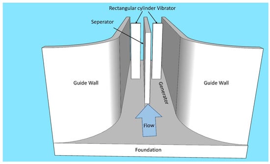
Figure 1.
Conceptual diagram of the VIVACE device.
The flow field around a rectangular cylinder in a narrow channel should be analyzed to maximize the energy harvesting efficiency of the device. However, no research has systematically investigated the effect of the blockage ratio, Reynolds number, and aspect ratio on the flow regime. Moreover, a few researchers [23] have studied the flow around a rectangular cylinder with an Ar < 1.0. However, the available studies indicate that the vortex shedding frequency will be greatly increased with an Ar < 1.0. Therefore, the flow around a rectangular cylinder with an Ar < 1.0 is critical to improving the VIVACE device.
Three rectangular cylinders with an Ar of 0.2, 0.3, and 0.5 were placed in a channel with a blockage ratio of 0.25. Furthermore, each rectangular cylinder was evaluated at flow velocities of 0.02, 0.04, and 0.1 m/s (the Re of the D is 1000, 2000, and 5000, respectively). The final objective is focused on studying the dynamic characteristics of the vortex-induced flow around the rectangular cylinder by analyzing the vortex shedding frequency, time-averaged flow field, Reynolds shear stress, space–time correlation, POD mode, and wall water pressure time-domain and frequency-domain characteristics.
2. Experimental Apparatus
This experiment’s self-circulating damping water sink was 4 m long, 0.6 m wide, and 1.8 m high, as shown in Figure 2. The sink consisted of an upstream tank, a diffusion section, a contraction section, a working section (1.5 m long, 0.2 m wide, and 0.3 m tall), and a tail tank. The honeycomb arrangements were located in the upstream tank. Holes were opened in the intake pipe wall and two buffers were placed below to decrease the flow turbulence. Furthermore, the contraction portion was fitted with three layers of honeycomb devices. The tailwater tank was linked to the output pipe with a conduit to decrease the influence of the pump’s vibration on the operating portion. Moreover, rubber shock absorbers were placed between the supports and the ground.
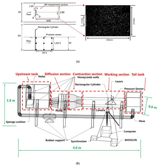
Figure 2.
Schematic diagram of the experimental setup: (a) Diagram of Pressure sensor arrangement and PIV window; (b) Overview of the experiment setep.
PIV was utilized to analyze the flow field of a slice 1 cm under the free water surface to better understand the development process of the vortex in the wake. A water pressure sensor array was also installed on the sidewall to investigate the pressure changes there. The combined usage of PIV and pressure sensors can also reflect the three-dimensional characteristics of the vortex to some extent.
Before being evaluated, the PIV flow field images and wall water pressure signals were pre-processed. The following measures were taken to improve the realism of the water pressure signal and the identifiability of the particles in the photos: (1) the background noise was removed from each photo by using the contrast approach; (2) Contrast-Limited Restricted Adaptive Histogram Equalization (CLAHE) was used to improve the local exposure; (3) an Intensity Highpass Filter (IHF) was used to remove uneven lighting; (4) an Intensity Capping Filter (ICF) was used to suppress the photo’s highlight signal and eliminate signal non-uniformity; and (5) noise from the water pressure signal was reduced using wavelet noise reduction. After pre-processing, the flow field was thoroughly studied in terms of the time-averaged flow field, Reynolds shear stress, space–time correlation, vorticity field, and water pressure time-frequency features. In particular, POD [24,25], a technique for analyzing massive amounts of data, was used to deconstruct the vorticity field. It has been applied in signal analysis, picture recognition, and stochastic processes. POD can be used in turbulence studies to associate coherent structures with the energy they contain, allowing researchers to detect diverse energy-level structures in turbulent environments.
In this investigation, we used plexiglass rectangular cylinders that were sharp-edged, 50 mm in height (D), and 10, 15, and 25 mm in width (B). Given that the rectangular cylinders were made of transparent plexiglass, a bright light band was generated following laser irradiation in a limited region in the neighborhood that concealed the tracer particles. Given that this study was not concerned with the flow in front of the rectangular cylinder, the start of the measuring area of the PIV was positioned at 0.1 D ahead of the trailing edge as shown in Figure 2a.
The PIV system was produced by Nanjing Hawksoft Technology Co. Ltd. A laser (MGL-N-532A) with a 532 nm wavelength was used to illuminate the flow field. The resolution of the industrial camera (JAI 5000 m cxp2) was 2354 × 1648 pixels. In this research, the processed window size was 100 × 100 pixels with 50% overlap, and the spatial resolution was 0.085 D. The HDPE particle diameter and density were 54 μm and 1.1 g/cm3, respectively. After calibration, the uncertainty of the system was ±2% in mean velocities. The sampling rate was 100 Hz, the Dt was 10 ms, and 6000 images were collected for each experiment. All of the images were analyzed after the experiments.
The precision of piezoresistive pressure transducers (Huaqiang sensor Technology Co.) is 0.1% (Figure 2b). A Jiangsu Donghua Test DH5922N multi-functional data acquisition device was used to capture the water pressure signal. A synchronizer was used to achieve synchronous acquisition using the PIV system.
3. Signal Pre-Processing
The measured data were pre-processed to verify the veracity of the information. The images taken by the camera were pre-processed to increase the probability that valid vectors would be identified. The measured pressure signal was then denoised to make it easier to analyze.
3.1. PIV Image Pre-Processing
PIV is a non-contact measurement technique for two-dimensional flow fields based on a cross-correlation analysis of flow field images and is widely used in various fields. The core of this technique is the identification of the tracer particle’s trajectory. Pre-processing was performed on the images taken by the camera before the flow field analysis was conducted in order to reduce interference and improve accuracy.
The two steps are as follows:
- Extract the common background noise in each set of two consecutive images, then remove it. As shown in Figure 3, (a) represents the unprocessed original picture; (b) represents the average intensity, also known as the background noise; and (c) represents the image produced after eliminating the background noise. The initial stage of processing was completed at this time. The effective vector identification rate was improved using several mathematical approaches in the second step.
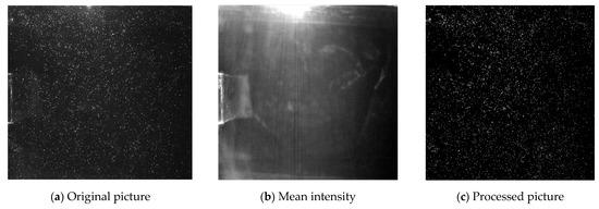 Figure 3. The effect of subtracting the mean intensity: (a) Original picture of the particles; (b) Subtracted mean intensity; (c) Picture of the particles without mean intensity.
- 2.
- Use CLAHE, IHF, and ICF to enhance the details in the photo further.
First, by using CLAHE, the image’s exposure was improved. The CLAHE technique benefits from not operating on the histogram of the entire picture, but rather on smaller sections (tiled images), optimizing each block by equalizing the contrast histogram. Consequently, the resultant distribution corresponded to a flat range of 0 to 255, and high exposure was tuned individually. Following histogram equalization, all neighboring blocks were merged using bilinear interpolation, resulting in no apparent borders between them. Shavit [26] found in their experiment that CLAHE could improve the detection probability of valid vectors. CLAHE re-maps the entire image, including the background noise; however, the background noise may be amplified, leading to PIV errors. Given that the background noise was reduced in the first step, the potential for this error was reduced.
Second, low-frequency background information generated by reflections from objects or uneven light was removed. An IHF was used to eliminate the interference. The IHF highlighted the particle information [27] in the picture while suppressing any low-frequency information. A high-pass filter was calculated by applying a low-pass filter to the image (blurring the image) and subtracting the result from the original image. An unsuitable threshold will cause the low-frequency movement to be lost.
Third, the ICF was used to suppress the signals of brilliant particles in the image to minimize non-uniformity. All particles in the interpretative frame were considered to have the same velocity during the identification of PIV vectors. However, a uniform flow is rare. Bright particles or bright spots inside the interpretative frame will contribute statistically more to the signal, biasing the results even more towards non-uniformity. The ICF was used to establish an upper limit of grayscale intensity, and this limit replaced all pixels over the threshold. Furthermore, combining an ICF with CLAHE increases the likelihood that vectors will be identified [26].
3.2. Pressure Signal Pre-Processing
Noise is unavoidable during signal measurement or transmission. Noise can be overlaid on the measured signal, affecting the original signal’s analysis. As a result, the observed signal must be denoised. In the wavelet domain, signals occur in the same locations with large magnitudes, whereas random noise appears inconsistently with small magnitudes, and systematic noise usually occurs at a specific location with a small magnitude. Mathematical approaches can be used to process the noise-containing signals in the wavelet domain. Wavelet denoising lowers the noise’s wavelet coefficients while retaining the original signal’s wavelet coefficients [28]. Compared with classic linear and nonlinear filtering approaches, wavelet denoising has superior time-frequency characteristics and accurately depicts the signal’s non-smoothness. Because of the great precision of the pressure sensor and the broad frequency response range, noise in the measurement process may be mixed. As a consequence, the wavelet denoising method was used to help with further analyses. Figure 4 depicts an ideal wavelet denoising outcome.
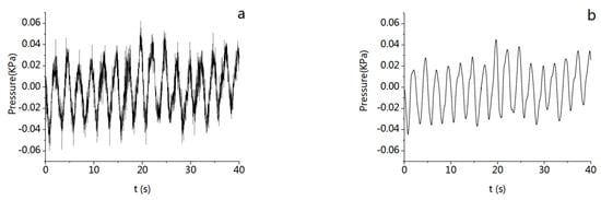
Figure 4.
Effect of wavelet denoising: (a) Original pressure signal with noise; (b) Denoised pressure signal.
4. Results and Discussion
4.1. Non-Dimensional Time-Average Streamwise Velocity and Reynolds Shear Stress
The non-dimensional time-averaged () velocity represents the trend of the shear layer and trailing region with Ar or Re. Figure 5 illustrates the non-dimensional time-averaged flow speed contour, y/D = 0 velocity profile, and spanwise velocity profile of the low-speed zone’s center under varying operating circumstances. Overall, the flow velocity was distributed symmetrically along the middle axis. The flow breaks from the plate’s leading edge, most of the flow spreads to the sides, and some of the flows interfere with each other in the trailing region, generating a low-velocity zone. When the Ar was the same, the breadth of the low-velocity zone steadily decreased as the Re increased. Furthermore, the middle portion of the low-velocity zone gradually closed to the plate, suggesting that the inertia of the water flow was increased, which corresponds to an increase in the Re. When the Re was constant, the low-velocity zone retained the same fluctuation features as the Ar increased, indicating that the extended plate slowed the formation of the shear layer.
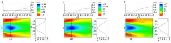
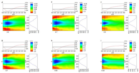
Figure 5.
Time-averaged streamwise velocity distribution: (a) Ar = 0.2, Re = 1000; (b) Ar = 0.3, Re = 1000; (c) Ar = 0.5, Re = 1000; (d) Ar = 0.2, Re = 2000; (e) Ar = 0.3, Re = 2000; (f) Ar = 0.5, Re = 2000; (g) Ar = 0.2, Re = 5000; (h) Ar = 0.3, Re = 5000; (i) Ar = 0.5, Re = 5000.
For all circumstances, the velocity profile along y/D = 0 revealed that the flow velocity tended to drop and subsequently rise. Furthermore, when the Ar = 0.2 and the Ar = 0.3, approached 0.5. When the Ar = 0.5, it tended to be 0.6.
With the increase in the Re, the range of the low-velocity zone was gradually reduced, and the center of the low-velocity zone gradually moved closer to the back of the rectangular cylinder. From Figure 5a,d,g, the velocity minima of the central axis appear at 1.1, 0.9, and 0.7 x/D. From Figure 5b,e,h, the velocity minima of the central axis appear at 1.05, 0.7, and 0.65 x/D. From Figure 5c,f,i, the velocity minima of the central axis appear at 0.8, 0.5, and 0.18 x/D. The spanwise velocity profile at the low-velocity zone’s center revealed that the flow velocity distribution was symmetric along y/D = 0. The flow velocity climbed slowly from the sidewall to the central axis, reached a peak at y/D = 1, and then dropped rapidly. The minimum was attained at y/D = 0. When the Ar = 0.5 and the Re = 5000, U/U0 in the wake area was positive, which means that no backflow existed in the time-averaged flow field. The causes of this occurrence will be addressed below.
The existence of the sidewall boundary layer, which limits the flow velocity near the sidewall, causes a sluggish increase in velocity in the spanwise velocity profile. Otherwise, the rectangular cylinder’s barrier creates a high-pressure zone upstream (deceleration layer and boundary layer) and a low-pressure wake region downstream (trailing region). The shear layer was located in the middle of the two areas, where the pressure varied considerably and the flow velocity increased. The gradual entry into the trailing area caused a rapid drop in flow velocity.
4.2. Reynolds Shear Stress Distribution
Reynolds stress is additional stress caused by a momentum exchange caused by turbulence and represent the turbulence intensity in the X and Y directions, respectively, that is, the energy component of turbulent pulsations, is the Reynolds shear stress, which represents the fluid momentum transport flux in turbulent flows and has a significant impact on the mean velocity profile. The Reynolds shear stress for each condition was investigated to understand the turbulence characteristics of the flow under different conditions. The effects of the Re and Ar on the flow field can be understood more clearly.
Figure 6 presents the Reynolds shear stress for various combinations of Re and Ar. The maximum and minimum values of Reynolds shear stress were found at the top and lower margins of the rectangular cylinder, respectively, which were axisymmetric as indicated in Figure 6. After the flow broke at the leading edge, antisymmetric stress bands appeared in the upper and lower edges. When the Ar was constant, the range of shear stress grew as the Re rose. Furthermore, an intense stress zone developed at the trailing edge. When the Re was unchanged, the range of shear stress expanded as the Ar increased, eventually reaching the center of the rectangular cylinder. The upper and lower edges of the following edge gradually roll up to the shear stress zone opposing the leading edge and extend downstream.
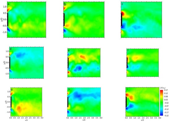
Figure 6.
Reynold shear stress distribution: (a) Ar = 0.2, Re = 1000; (b) Ar = 0.3, Re = 1000; (c) Ar = 0.5, Re = 1000; (d) Ar = 0.2, Re = 2000; (e) Ar = 0.3, Re = 2000; (f) Ar = 0.5, Re = 2000; (g) Ar = 0.2, Re = 5000; (h) Ar = 0.3, Re = 5000; (i) Ar = 0.5, Re = 5000.
No reflux was observed in the time-averaged flow field for an Ar = 0.5 and a Re = 5000, as previously stated. The explanation for this occurrence was that the shear stress zone rolled up towards the trailing edge, away from the rear of the rectangular cylinder, as shown in Figure 6i. The shear layer in the near-plate area did not interact with the tail flow. As a result, no stable reflux zone emerged in the trailing region.
The reason for the expansion in the spectrum of Reynolds shear stress bands as the Ar and Re increased was revealed. On the one hand, the increasing Ar reduced the contact between the separated shear layers, and the flow tended to reconnect itself to the rectangular cylinder following separation at the leading edge. On the other hand, the rise in the Re caused an increase in the flow’s turbulence and a natural increase in the Reynolds shear stress, which was comparable to the results reported by Narasimhamurthy [29].
4.3. Space–Time Correlation Analysis
Space–time correlation analysis was utilized to better understand the vortex transport mechanism in the trailing area. A reference point was set in the wakefield (x0, y0), and the coordinates of the remaining points on the same horizontal line (x0 + r, y0) were calculated. Thus, at this moment, the non-dimensional space–time correlation function of the streamwise velocity fluctuation component u′ is as follows:
According to the above-described Reynolds shear stress distribution characteristics, and the large-scale vortex structure generation, shedding, and transport process, the coordinates of the reference point are (x/D = 0.426, y/D = −0.489). According to the reference point, the space–time correlation contours of the streamwise fluctuation velocity of nine sets of circumstances were created.
The horizontal coordinate in Figure 7 is the non-dimensional delay time , and the vertical coordinate is the non-dimensional position x/D. As a result, the physical means of each point in the figure were the correlation coefficient between the streamwise fluctuation velocity u′ of any streamwise position and the streamwise fluctuation velocity u′0 of the reference point at any time, respectively.
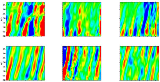
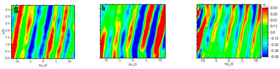
Figure 7.
Space–time contour plots of streamwise velocity: (a) Ar = 0.2, Re = 1000; (b) Ar = 0.3, Re = 1000; (c) Ar = 0.5, Re = 1000; (d) Ar = 0.2, Re = 2000; (e) Ar = 0.3, Re = 2000; (f) Ar = 0.5, Re = 2000; (g) Ar = 0.2, Re = 5000; (h) Ar = 0.3, Re = 5000; (i) Ar = 0.5, Re = 5000.
The regions with a high positive and negative correlation coefficient between u′ and u′0 are denoted by bright red stripes and bright blue stripes, respectively. Calculating the slope of the brilliant stripes yields the vortex transfer velocity. Certain stripes in the picture are broken up or not continuous, indicating that the vortex transport was unstable or that some vortices were connected.
St is a critical metric that reflects the frequency of vortex shedding. The geometric shape, feature size, and Br are all intimately related to St. Figure 8 depicts several researchers’ variations in the St with the Ar and Br. The St falls significantly as the Ar increases, but just somewhat as the Re increases, which is similar to the findings of Igarashi [23] and Wang [20]. As indicated in the graph, when the Br grew from 0.067 to 0.25, the St increased by almost 25%. Furthermore, when the Ar decreased from 0.5 to 0.2, the St increased by approximately 25%. In addition, as the Ar and Re grew, so did the non-dimensional vortex transport velocity .
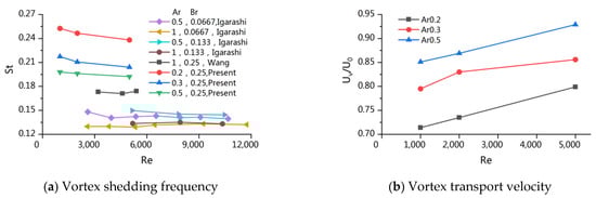
Figure 8.
Characteristics of shedding vortexes: (a) the variation in the Strouhal number with the Ar and Br obtained by different researchers; (b) the non-dimensional vortex transport velocity obtained in this research.
Because of the elongation of the plate in the streamwise direction, the St dramatically fell as the Ar increased. The interaction between the separated shear layers was disrupted, resulting in rapid vortex shedding. Meanwhile, the obstruction inhibited the shear layer’s spanwise development, accelerating the free stream and increasing the vortex shedding frequency.
4.4. Proper Orthogonal Decomposition Analysis
When studying complex space–time variation problems, the POD technique is always utilized. The core idea of the POD method is to find the optimal space of orthogonal basis functions in the mean square sense from a time series of spatial data, and to obtain an approximate description of the higher-order data with fewer orthogonal basis expansions, as follows:
Select N transient velocity fields, define vi to represent the i-th velocity field, build a snapshot set of N transient velocity fields in the database, and write the snapshot as the sum of the average value and the fluctuation amount:
using to build a time series of spatial data, discover a set of appropriate orthogonal bases {= 1, 2, … N} to establish the mapping , and minimize the error between the original system and the reduced system projected on the orthogonal bases:
this problem is equivalent to the problem of maximizing the orthogonal basis functions:
where signifies the space of functions defined on the space area ; denotes the inner product on this function space; ; and denotes the average arithmetic operation.
This maximum problem can be turned into an eigenvalue problem using the variational method:
where is the autocorrelation function of u, commonly known as the POD kernel,, and this eigenvalue problem generates the POD mode, which is the corresponding eigenvector.
Because snapshots represent the outputs of experimental data or numerical simulations at discrete spatial positions in practice, the autocorrelation function can be stated as follows:
In this study, the spatial scale was much larger than the time scale. The Snapshot-POD was used to speed up the calculation. The main idea of this method is to use the original function’s space elements in the same linear space as the eigenmodes in the eigenvalue problem. In this way, the eigenmodes can be represented by the linear combination of the original function’s space snapshots:
substituting Equation (7) into Equation (5), we obtain , where is the eigenfunction corresponding to the eigenvalue λi:
the to-be-solved eigenvalue problem is only of order N, which is substantially smaller than the space point M. Solve the eigenvalues and eigenvectors of the correlation matrix R to yield the POD model.
The flow field was first decomposed by the Karhumen–Loeve expansion in this work. The proposed large-scale order structure in the flow field was discovered by computing the modes based on the energy ratio. Distinct flow modes were analyzed to determine the effect of the Re and Ar on the flow. The analysis was carried out under the nine conditions listed above.
The turbulent energy ratio of 1000 modes derived from the flow velocity is shown in Figure 9. The first two modes’ energy accounted for more than 75% of the turbulent kinetic energy. The turbulent kinetic energy of higher modes, which characterize the flow’s small-scale structure, fell rapidly as the modal order increased. As the Re and Ar increased, the turbulent kinetic energy occupied by lower modes increased to varying degrees and shifted to higher-order modes. The turbulence intensity of the entire flow was raised by activating the flow field’s small-scale structure.
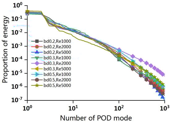
Figure 9.
Energy distribution of the POD modes.
Figure 10, Figure 11 and Figure 12 display the vortex modal contour of each order for each combination of Ar and Re. The first, second, and third rows represent the mean vorticity field, the first-order vortex mode, and the second-order vortex mode, respectively. Furthermore, the black circles in the contours depict the vortex structure in the flow field as determined by the Q-criterion.
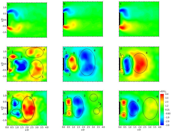
Figure 10.
The modes of Proper Orthogonal Decomposition of Ar = 0.2: (a) Re = 1000, the zeroth-order mode (mean vorticity field); (b) Re = 2000, the zeroth-order mode (mean vorticity field); (c) Re = 5000, the zeroth-order mode (mean vorticity field); (d) Re = 1000, the first-order mode; (e) Re = 2000, the first-order mode; (f) Re = 5000, the first-order mode; (g) Re = 1000, the second-order mode; (h) Re = 2000, the second-order mode; (i) Re = 5000, the second-order mode.
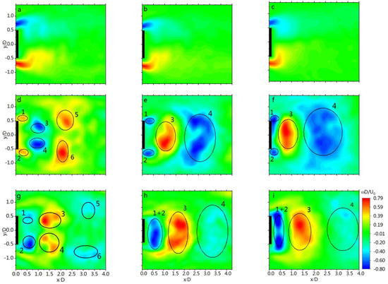
Figure 11.
The modes of Proper Orthogonal Decomposition of Ar = 0.3: (a) Re = 1000, the zeroth-order mode (mean vorticity field); (b) Re = 2000, the zeroth-order mode (mean vorticity field); (c) Re = 5000, the zeroth-order mode (mean vorticity field); (d) Re = 1000, the first-order mode; (e) Re = 2000, the first-order mode; (f) Re = 5000, the first-order mode; (g) Re = 1000, the second-order mode; (h) Re = 2000, the second-order mode; (i) Re = 5000, the second-order mode.
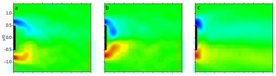
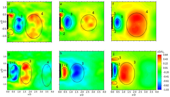
Figure 12.
The modes of Proper Orthogonal Decomposition of Ar = 0.5: (a) Re = 1000, the zeroth-order mode (mean vorticity field); (b) Re = 2000, the zeroth-order mode (mean vorticity field); (c) Re = 5000, the zeroth-order mode (mean vorticity field); (d) Re = 1000, the first-order mode; (e) Re = 2000, the first-order mode; (f) Re = 5000, the first-order mode; (g) Re = 1000, the second-order mode; (h) Re = 2000, the second-order mode; (i) Re = 5000, the second-order mode.
In the overview of Figure 10, two distinct vortexes emerged in the trailing zone. Furthermore, the zeroth-order mode (time-averaged vorticity field) revealed two stable arc vortex bands beginning at the leading edge, demonstrating basic symmetry. In the first-order mode, two vortices developed at each trailing edge corner and propagated downstream with progressive energy dissipation. The flow structure in the second-order mode was comparable to that in the first-order mode, but had a phase difference. The flow configuration in Figure 10g is similar to that in Figure 10d, except that the vortexes along the trailing edge (#1 and #2) were totally detached from the plate. Furthermore, vortexes #4 and #5 vanished. The vortex band shown in Figure 10b had a bigger arc and a wider range when the Re = 2000. The first-order mode had four vortexes, with vortex #4 corresponding to vortexes #5 and #6 in Figure 10d. In Figure 10h, vortex #4 is separated into two low-energy vortexes. When the Re = 5000, the vortex structures were the same as the one when the Re = 2000. However, the vortex band shown in Figure 10c had a bigger arc and a larger range, and vortexes #1 and #2 separated even more. Vortexes #3 and #4 had the largest power. Vortex #4 was still evident, as shown in Figure 10i.
The vortex structures shown in Figure 11 were similar to those shown in Figure 10 with the following exceptions: (1) the arc and range of the vortex bands in the zeroth-order mode were larger than those in Figure 10; (2) vortexes #3 and #4 in Figure 11d,g (i.e., the second POD mode) matched to the unseparated vortex #3 in Figure 10d,g; and (3) in the second POD mode, vortexes #1 and #2 were united into one vortex.
Compared with the vortex structures shown in Figure 11, those shown in Figure 12 have important differences. First, the arc of the vortex bands in the zeroth-order mode was larger The vortex bends’ tail closed in on the trailing edge of the rectangular cylinder. The vortex bends, in particular, evolved into a vortex cluster on the trailing edge’s two corner points. Second, when the Re = 1000, vortexes #1 and #2 in Figure 12c were united into one vortex in the second POD mode. Third, in Figure 12i, two new high-vorticity zones (i.e., #5 and #6) emerged on two sides of the rectangular cylinder as a result of the greater flow velocity in these two locations, rather than the true vortex.
When the Re and Ar were small, the flow structures became unstable quickly as a result of inter-vortex swallowing, tearing, and merging. However, with the increase in the Re, the distance of steady propagation of the vortex structure increased. Furthermore, the tail of the vortex band in the time-averaged vorticity field approached the rectangular cylinder gradually. Moreover, two vortices formed two sharp corners on the back of the rectangular cylinder. In addition, as the Ar increased, the trailing edge of the rectangular cylinder interfered with the interaction of shear layers, consistent with the previous conclusion on the Reynolds shear stress.
4.5. Pressure Fluctuation Characteristics
The vortex shedding of the rectangular cylinder will affect the water pressure on the sink’s sidewall. By examining the wall pressure characteristics, the properties of vortex transport might be discovered.
The signal eigenvalues in the time domain were computed and analyzed. As shown in Figure 13, the root mean square (RMS) values of the varying pressure on the sidewall were studied. The following are some of the results that were obtained. First, in a vertical plane that is the same, the RMS of the pressure fluctuation dropped as the water depth increased at x/d = 0.1 d, and the RMS increased as the water depth climbed at x/d = 1.1 d. However, when x/d = 2.1 d, the RMS value was at its lowest at the center of the sink. The incipient vortex was funnel-shaped, and it swung along the lateral direction during transit downstream. Furthermore, the swing speed was not consistent along the vertical axis. Second, when the Re remained constant, the RMS of the pressure fluctuation rose as the Ar increased. This suggests that the vortex’s range and intensity had grown. Third, when the Ar was constant, the RMS fell as the Re increased. Due to the strengthening of inertia, the vortexes tended to move downstream of the plate rather than to the sides. The variation in Ar had little effect on the transport characteristics of the vortexes.
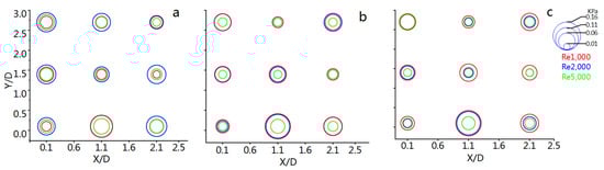
Figure 13.
RMS of the fluctuating pressure: (a) Ar = 0.2; (b) Ar = 0.3; (c) Ar = 0.5.
Finally, the frequency characteristics of the varying pressure on the sidewall were determined. The power spectrum of fluctuating pressure signals under various conditions at certain representative places of measurement was calculated and is presented in Figure 14. As the Ar increased, the main frequency fell, and the energy declined proportionately. Under the same operating conditions, the frequency spectra of each measurement point were very similar. There was a strong association between the primary frequency and the vortex shedding frequency.
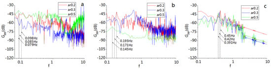
Figure 14.
Power spectrum of fluctuating pressure signals: (a) Re = 1000; (b) Re = 2000; (c) Re = 5000.
5. Conclusions
This study systematically examined the flow around a rectangular cylinder by testing in an open channel a sink with a blockage effect. The impacts of the Ar and Re on the turbulence in the structure were considered. The flow field data presented in this article were collected by using a PIV system and a water pressure sensor and were then analyzed by using POD analysis and the wavelet noise reduction method. The flow around a rectangular cylinder in an open channel and the impacts of the Ar, Br, and Re on the flow field structure were thoroughly investigated. The time-averaged flow field, Reynolds shear stress, space–time correlation, vorticity field, and water pressure characteristics were used to investigate the impacts. The main conclusions are as follows:
1. Approximately 75% of the total energy was accounted for by the first two orders of POD mode energy. The first two modes were capable of detecting the large-scale vortex structure. The primary wall water pressure frequency and the vortex shedding frequency were highly consistent. As a result, vortex shedding was the primary source of variations in the wall water pressure.
2. The vortex water flowing around a rectangular cylinder always creates two antisymmetric vortices at the upper and lower ends of the leading edge and then travels downstream, according to the POD modes. The vortices conveyed downstream take diverse forms depending on the Ar and Re, then propagate independently of dissipation. Alternatively, the two vortices alternately travel along the central axis, resulting in the merger of the second or third-order POD modes.
3. The difference in the Ar (or Re) significantly impacts the range of the low-velocity zone and the distribution of the Reynolds shear stress in the wake region. The low-velocity zone in the wake, symmetrically distributed along the central axis, diminishes as the Ar and Re increase. As the Ar and Re increased, the extreme value zone of the Reynolds shear stress steadily migrated toward the trailing edge of the rectangular cylinder. When the Ar = 0.5 and the Re = 5000, no stable reflux zone formed in the low-velocity zone because of the excessive shear stress zone distant from the rectangular cylinder. The results of the POD analysis also support this pattern.
4. The vortex shedding frequency can be greatly increased by increasing the blocking ratio and decreasing the chord thickness ratio of the rectangular cylinder. As the Ar increased, the St decreased dramatically. The vortex shedding frequency fell as the rectangular cylinder elongated, causing the trailing edge to interfere with the formation of the shear layer. When the Re = 1000 and the Ar = 0.2, the maximum value was 0.253. However, as the Ar and Re grew, so did the associated non-dimensional vortex transport velocity, reaching a maximum of 0.93 U0 for Ar = 0.5 and Re = 5000. The blocking effect slowed the formation of the shear layer and hastened the vortex shedding. Compared with Igarashi’s work, increasing the Br from 0.067 to 0.25 enhanced the St by 25%.
5. The combination of the PIV system and a pressure sensor revealed the three-dimensional characteristics of vortex shedding from the rectangular cylinder to some extent. The peculiarities of the water pressure revealed the vortices’ properties. During downstream transport, the incipient vortex was funnel-shaped and swung along the lateral direction (with varying swing velocities along the vertical direction). The RMS pressure rose as the Ar increased, implying that the vortex intensity increased. Furthermore, the vortex favored downstream transfer rather than spanwise transport.
Therefore, for a waterway with low velocity, a rectangular cylinder with an aspect ratio of 0.2 should be placed in a confined channel with a 0.25 blockage ratio in order to capture the combined strengths of wakes and vortices, which may be extremely useful in enhancing the efficiency of the VIVACE device. The increase in the vortex shedding frequency and local flow velocity was most pronounced at a flow rate of 0.1 m/s. These experimental results could constitute a reference for further VIVACE device tests.
Author Contributions
Conceptualization, X.S.; writing—original draft preparation, X.S.; writing—review and editing, J.D.; supervision, G.Y.; validation, C.Z. All authors have read and agreed to the published version of the manuscript.
Funding
This research received no external funding.
Institutional Review Board Statement
Not applicable.
Informed Consent Statement
Not applicable.
Data Availability Statement
Not applicable.
Acknowledgments
The kind help of Bo Wu during the submission should be acknowledged.
Conflicts of Interest
The authors declare no conflict of interest.
Nomenclature
| Lists of symbols | |
| Re | Reynold number = ρU0D/μ |
| B | the width of a rectangular cylinder |
| D | the height of a rectangular cylinder |
| Ar | aspect ratio = B/D |
| Br | blockage ratio |
| f | vortex shedding frequency |
| U0 | free flow velocity |
| u′ | fluctuation x velocity |
| v′ | fluctuation y velocity |
| non-dimensional Reynolds stress | |
| non-dimensional Reynolds stress | |
| non-dimensional | |
References
- Baranya, S.; Olsen, N.R.B.; Stoesser, T.; Sturm, T. Three-dimensional rans modeling of flow around circular piers using nested grids. Eng. Appl. Comp. Fluid 2012, 6, 648–662. [Google Scholar] [CrossRef] [Green Version]
- Liu, M.; Chiang, W.; Hwang, J.; Chu, C. Wind-induced vibration of high-rise building with tuned mass damper including soil-structure interaction. J. Wind Eng. Ind. Aerodyn. 2008, 96, 1092–1102. [Google Scholar] [CrossRef]
- Chen, K.; Chen, Y.; She, Y.; Song, M.; Wang, S.; Chen, L. Construction of effective symmetrical air-cooled system for battery thermal management. Appl. Therm. Eng. 2020, 166, 114679. [Google Scholar] [CrossRef]
- Zhu, H.; Zhao, Y.; Zhou, T. Numerical investigation of the vortex-induced vibration of an elliptic cylinder free-to-rotate about its center. J. Fluid Struct. 2018, 83, 133–155. [Google Scholar] [CrossRef]
- Rigo, F.; Denoël, V.; Andrianne, T. Vortex induced vibrations of rectangular cylinders arranged on a grid. J. Wind Eng. Ind. Aerodyn. 2018, 177, 327–339. [Google Scholar] [CrossRef] [Green Version]
- Yildizdag, M.E.; Ardic, I.T.; Demirtas, M.; Ergin, A. Hydroelastic vibration analysis of plates partially submerged in fluid with an isogeometric FE-BE approach. Ocean Eng. 2019, 172, 316–329. [Google Scholar] [CrossRef]
- Bernitsas, M.M.; Raghavan, K.; Ben-Simon, Y.; Garcia, E.M.H. VIVACE (vortex induced vibration aquatic clean energy): A new concept in generation of clean and renewable energy from fluid flow. J. Offshore Mech. Arct. 2008, 130, 0411014. [Google Scholar] [CrossRef]
- Wu, W.; Sun, H.; Lv, B.; Bernitsas, M.M. Modelling of a hydrokinetic energy converter for flow-induced vibration based on experimental data. Ocean Eng. 2018, 155, 392–410. [Google Scholar] [CrossRef]
- Wang, D.; Chiu, C.; Pham, H. Electromagnetic energy harvesting from vibrations induced by Kármán vortex street. Mechatronics 2012, 22, 746–756. [Google Scholar] [CrossRef]
- Kuila, A.; Das, S.; Mazumdar, A. Turbulence Spectrum Around a Suspended Cylinder with Vertical Endplate Effects to Enhance VIVACE Strength. J. Waterw. Port Coast. Ocean. Eng. 2021, 147, 040210245. [Google Scholar] [CrossRef]
- Lee, J.H.; Bernitsas, M.M. High-damping, high-Reynolds VIV tests for energy harnessing using the VIVACE converter. Ocean Eng. 2011, 38, 1697–1712. [Google Scholar] [CrossRef]
- Guissart, A.; Andrianne, T.; Dimitriadis, G.; Terrapon, V.E. Numerical and experimental study of the flow around a 4:1 rectangular cylinder at moderate Reynolds number. J. Wind Eng. Ind. Aerodyn. 2019, 189, 289–303. [Google Scholar] [CrossRef] [Green Version]
- Hemmati, A.; Wood, D.H.; Martinuzzi, R.J. On simulating the flow past a normal thin flat plate. J. Wind Eng. Ind. Aerodyn. 2018, 174, 170–187. [Google Scholar] [CrossRef]
- Tenaud, C.; Podvin, B.; Fraigneau, Y.; Daru, V. On wall pressure fluctuations and their coupling with vortex dynamics in a separated–reattached turbulent flow over a blunt flat plate. Int. J. Heat Fluid Flow 2016, 61, 730–748. [Google Scholar] [CrossRef] [Green Version]
- Parker, R.; Welsh, M.C. Effects of sound on flow separation from blunt flat plates. Int. J. Heat Fluid Flow 1983, 4, 113–127. [Google Scholar] [CrossRef]
- Nakamura, Y.; Ohya, Y.; Ozono, S.; Nakayama, R. Experimental and numerical analysis of vortex shedding from elongated rectangular cylinders at low Reynolds numbers 200-10(3). J. Wind Eng. Ind. Aerodyn. 1996, 65, 301–308. [Google Scholar] [CrossRef]
- Cherry, N.J.; Hillier, R.; Latour, M.E.M.P. Unsteady measurements in a separated and reattaching flow. J. Fluid Mech. 1984, 144, 13–46. [Google Scholar] [CrossRef]
- Fukuda, K.; Balachandar, R.; Barron, R.M. Development of vortex structures in the wake of a sharp-edged bluff body. Phys. Fluids 2017, 29, 125103. [Google Scholar] [CrossRef]
- Shi, L.L.; Liu, Y.Z.; Yu, J. PIV measurement of separated flow over a blunt plate with different chord-to-thickness ratios. J. Fluid Struct. 2010, 26, 644–657. [Google Scholar] [CrossRef]
- Wang, X.; Chen, J.; Zhou, B.; Li, Y.; Xiang, Q. Experimental investigation of flow past a confined bluff body: Effects of body shape, blockage ratio and Reynolds number. Ocean Eng. 2021, 220, 108412. [Google Scholar] [CrossRef]
- Chakrabarty, D.; Brahma, R. Fluid flow and heat transfer characteristics for a square prism (blockage ratio=0.1) placed inside a wind tunnel. Heat Mass Transf. 2008, 44, 325–330. [Google Scholar] [CrossRef]
- Yang, G.; Yong, Q.; Ming, G.U. Large Eddy Simulation of Blockage Effect on Flow Past a Two Dimensional Square Cylinder. J. Tongji Univ. 2018, 46, 1018–1025. [Google Scholar]
- Igarashi, T. Fluid flow and heat transfer around rectangular cylinders (the case of a width/height ratio of a section of 0.33~1.5). Int. J. Heat Mass Transf. 1987, 30, 893–901. [Google Scholar] [CrossRef]
- Hu, R.; Liu, Y. Proper orthogonal decomposition of turbulent flow around a finite blunt plate. J. Vis. Jpn. 2018, 21, 763–777. [Google Scholar] [CrossRef]
- Fujiwara, K.; Sriram, R.; Kontis, K. Experimental investigations on the sharp leading-edge separation over a flat plate at zero incidence using particle image velocimetry. Exp. Fluids 2020, 61, 9. [Google Scholar] [CrossRef]
- Shavit, U.; Lowe, R.J.; Steinbuck, J.V. Intensity Capping: A simple method to improve cross-correlation PIV results. Exp. Fluids 2007, 42, 225–240. [Google Scholar] [CrossRef]
- Thielicke, W.; Sonntag, R. Particle Image Velocimetry for MATLAB: Accuracy and enhanced algorithms in PIVlab. J. Open Res. Softw. 2021, 9, 1. [Google Scholar] [CrossRef]
- Srivastava, M.; Anderson, C.L.; Freed, J.H. A New Wavelet Denoising Method for Selecting Decomposition Levels and Noise Thresholds. IEEE Access 2016, 4, 3862–3877. [Google Scholar] [CrossRef] [PubMed]
- Narasimhamurthy, V.D.; Andersson, H.I. Numerical simulation of the turbulent wake behind a normal flat plate. Int. J. Heat Fluid Flow 2009, 30, 1037–1043. [Google Scholar] [CrossRef]
Publisher’s Note: MDPI stays neutral with regard to jurisdictional claims in published maps and institutional affiliations. |
© 2021 by the authors. Licensee MDPI, Basel, Switzerland. This article is an open access article distributed under the terms and conditions of the Creative Commons Attribution (CC BY) license (https://creativecommons.org/licenses/by/4.0/).