1. Introduction
Large-scale hydrologic model predictions can address many grand water challenges, such as flood, drought, and climate change predictions. These modeling approaches are constantly challenged by the need to represent smaller-scale processes and heterogeneities, yet cover large relevant domains while being computationally efficient. As pointed out recently [
1,
2], increases in model resolution are often needed to make large-scale predictions relevant for a local policy decision. However, the computational cost of these models is large [
1], resulting in long run times even for modern supercomputers [
3,
4]. Several approaches are being leveraged to accelerate this process, including graphical processing unit (GPU) architectures [
5,
6]; however, further acceleration will enable more a locally relevant simulation. In recent years, there have been tremendous developments in the use of machine learning emulators for complex physical problems as a way to accelerate complex and high-fidelity physical models [
7,
8,
9].
Deep learning (DL) tools are increasingly used in earth sciences and in hydrology in particular to predict precipitation [
10,
11,
12,
13,
14], streamflow [
15,
16,
17,
18,
19,
20], and groundwater [
21,
22,
23,
24,
25,
26]. These prior applications fall into two categories: spatially based and temporally based. Spatially based approaches (e.g., convolutional neural network (CNN)) learn dynamical features of hydrological component(s) from the surrounding dynamical fields by using a hierarchical set of spatial convolution kernels. CNN models have been used, for example, to simulate short- to medium-term precipitation events [
27,
28]. Temporally based approaches (e.g., recurrent neural network (RNN)) learn the temporal dynamic behavior of a process or event [
15,
16]. With these recurrent connections, temporally based approaches can represent the long memory present in hydrologic systems; however, they are limited to point-scale predictions.
For a DL approach to be a meaningful emulator of large-scale hydrologic models, the spatially and temporally based approaches need to be combined. However, efforts to combine these two approaches are still at an early stage. One such effort is the convolutional long short-term-memory (ConvLSTM) method [
29] that combines spatial and temporal autocorrelations. ConvLSTM has demonstrated better performance than CNN [
30] and LSTM [
29] individually, particularly on video interpolation and extrapolation. However, as the lead in prediction time increases, the vanishing gradient problem (see
Section 2.2) of RNNs decreases the prediction accuracy [
29], something overcome in recent applications: predictive recurrent neural network (PredRNN [
31,
32]).
Here, we detail the development of a deep learning emulator for the integrated hydrologic model ParFlow [
33]. The emulator is built using the PredRNN model [
31,
32]. We train the emulator based on simulation results from ParFlow. This emulator takes ParFlow model parameters (e.g., topographic slopes, saturated hydraulic conductivity tensors, and initial pressure) and rainfall information as inputs and produces three-dimensional transient outputs (e.g., pressure head and saturation). We conduct simulations using different rainfall–runoff scenarios in two realistic setups, the Taylor River basin in the Rocky Mountains and the Little Washita basin in Southwestern Oklahoma.
2. Materials and Methods
In this section, we briefly introduce the ParFlow model and equations. Then we present the DL model, PredRNN, used to construct the ParFlow emulator.
2.1. The Integrated Hydrologic Model, ParFlow
We use the integrated hydrologic model ParFlow [
34,
35,
36,
37,
38] to simulate the response of a pressure head resulting from synthetic rainfall scenarios. ParFlow computes subsurface fluxes and surface fluxes by solving the three-dimensional Richards equation [
39] and two-dimensional kinematic wave equations. Subsurface and surface fluxes are integrated using a free surface overland flow boundary condition.
The Richards equation for a variably saturated flow is given as [
37]:
where
is the pressure head (L),
is the elevation (L),
is the specific storage (L
−1),
is the relative saturation (–),
is the porosity (–),
is the saturated hydraulic conductivity tensor (LT
−1),
is the relative permeability (–),
is a sink/source term (T
−1), and
is the local angle of a topographic slope (S). The overland flow equation is given as [
36,
38]:
where
is the unit vector in the vertical (–),
denotes the maximum of the two quantities,
is the two-dimensional depth-averaged surface water velocity (LT
−1), and
is a constant equal to the inverse of the grid scaling (L
−1) [
38].
The van Genuchten [
40] equations are used to relate relative saturation to water head given as:
where α (L
−1) and
n (–) are soil parameters,
ssat (–) is the relative saturated water content, and
sres (–) is the relative residual saturation.
2.2. The Emulator Version of ParFlow, ParFlow-ML
The emulator model (ParFlow-ML) is constructed using a predictive recurrent neural network (PredRNN) developed by Wang et al. [
31,
32]. The PredRNN architecture has two major components: (1) a new spatiotemporal memory mechanism, called causal LSTM, to increase the short-term modeling capacity, and (2) the gradient highway recurrent unit (GHU) to capture the influence of long-term information.
In a causal LSTM, the recurrence depth is increased along the spatiotemporal transition pathway (
Figure 1), which includes dual memories, the temporal memory
and the spatial memory
. The GHU is based on a study by Srivastava et al. [
41], which indicates that highway layers can deliver gradients efficiently in deep feed-forward networks. The structure of the GHU is shown with the final PredRNN architecture in
Figure 2; equations of the GHU are as follows:
Here,
are the convolutional filters,
are the transformed inputs, and
are the hidden states.
is named as switch gate, which enables an adaptive learning between the transformed inputs and the hidden states [
31]. In the final PredRNN architecture, the GHU enables an alternative quick route from the first to the last timestep (the blue line in
Figure 2). These two components enable the PredRNN to learn complex video sequence dynamics and predict state-of-the-art results [
31,
32]. The first component, the causal LSTM with a cascade dual memory structure, enhances the ability of the PredRNN to capture short-term dynamics. The second component, the GHU, which links future predictions to distant inputs, alleviates the vanishing gradient problem.
2.3. Experiment Design
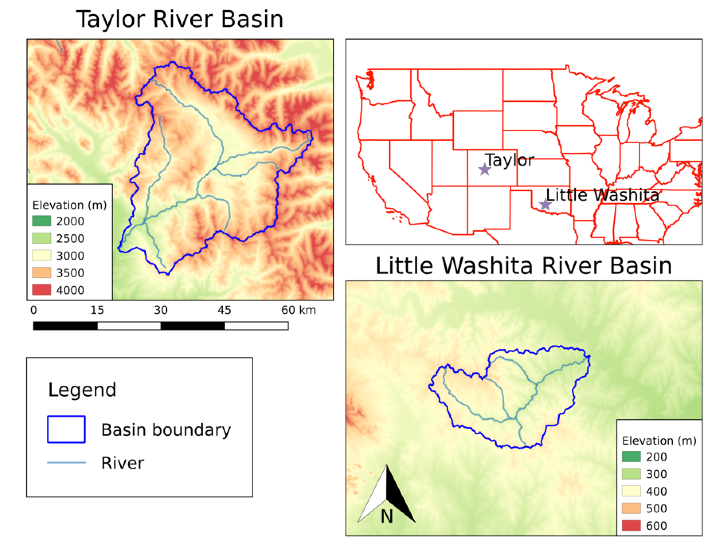
We train the emulator on two different river basins, the Taylor and Little Washita. In this section, we discuss the study areas, the emulator setup, the hydrologic model setup, and the rainfall–runoff scenarios.
2.3.1. Study Areas
The two modeling domains used in this study are the Taylor River basin and the Little Washita basin (
Figure 3). The Taylor River basin, located in the Rocky Mountains, has an area of 1236 km
2 and a mean elevation of 3500 m (
Figure 3). The outlet of the basin is located at Almont, Colorado, USA. The Little Washita basin, located in the Southwestern Oklahoma, has an area of 600 km
2 and is characterized by rolling terrain. The outlet of the basin is located at Smithville, Oklahoma, USA.
2.3.2. The Emulator Setup
The emulator, ParFlow-ML, is trained with ParFlow’s inputs to predict ParFlow outputs of the pressure head and relative saturation. There are two types of ParFlow inputs: static inputs (discussed in
Section 2.3.3) and dynamic inputs (discussed in
Section 2.3.4). Static inputs include surface and subsurface information, such as topographic slopes, Manning’s roughness values, saturated hydraulic conductivity tensors, and domain’s initial pressure. Static inputs are used as the initial spatial memory
for ParFlow-ML. ParFlow’s rainfall information is used as the dynamic input for ParFlow-ML. For each dynamic input timestep, ParFlow-ML outputs the corresponding pressure head and relative saturation.
2.3.3. Model Setup
In this study, the model setups are the same for the Taylor River basin and the Little Washita River basin. Both model setups include five vertical layers that are 0.1, 0.3, 0.6, 1.0, and 100 m thick. The two basins are implemented with a lateral resolution of 1 km. Model inputs consist of two types of data: surface and subsurface.
The surface inputs, topographic slopes and land cover, are evaluated as follows. Topographic slopes are calculated from the elevation input from the hydrological data and maps based on shuttle elevation derivatives at multiple scales (HydroSHEDS) using the priority flow toolbox [
42]. The land cover characteristic is upscaled from the original 30 m resolution National Land Cover Database (NLCD).
The subsurface inputs include four soil layers at the top and one geological layer at the bottom, including soil and geological layer characteristics, such as saturated hydraulic conductivity and van Genuchten parameters [
43]. Soil and geological layer categories were taken from the Soil Survey Geographic Database (SSURGO) and from a global permeability map developed by Gleeson et al. [
44]. More details about the subsurface inputs and their configuration can be found in Maxwell et al. [
38] and Maxwell and Condon [
45].
2.3.4. Rainfall–Runoff Scenarios
To simulate rainfall–runoff simulations using ParFlow, we specify a “rainfall–recession” cycle as a boundary condition for the top of the simulation domain. Rain length and rain frequency can be specified by setting two ParFlow input keys, Cycle.rainrec.rain.Length and Cycle.rainrec.rec.Length, respectively. Rain values can be specified by setting the Patch.top.BCPressure.rain.Value input key. ParFlow outputs the pressure head, and relative saturation files consist of five layers.
To have random boundary conditions as forcing of the simulation, the 24 rainfall scenarios with varying rain intensities (
I), rain lengths (
RL), and rain frequencies (
RecL) (
Table 1) were divided into three sets, namely, the
train set (scenarios 1–16;
Figure 4a), the
validation set (scenarios 17–20;
Figure 4b), and the
test set (scenarios 21–24;
Figure 4c).
I,
RL, and
RecL are chosen uniformly from three respective ranges of 0.01–0.08 m/h, 5–30 h, 15–60 h. Each rainfall–runoff scenario is unique and independent from one another. With a rainfall length ranging between 5 and 30 h and a simulation period of 120 h, there would be 1 to 3 rainfall events and 1 to 4 peak flows in each scenario. Scenarios included in the
train set have both single and multiple peak flows whose magnitudes vary from 5000 m
3/s (scenario 8) to 22,000 m
3/s (scenarios 15). Scenarios included in the
validation and
test sets also have multiple peak flows whose magnitudes vary from 7000 m
3/s (scenario 18) to 21,000 m
3/s (scenario 23).
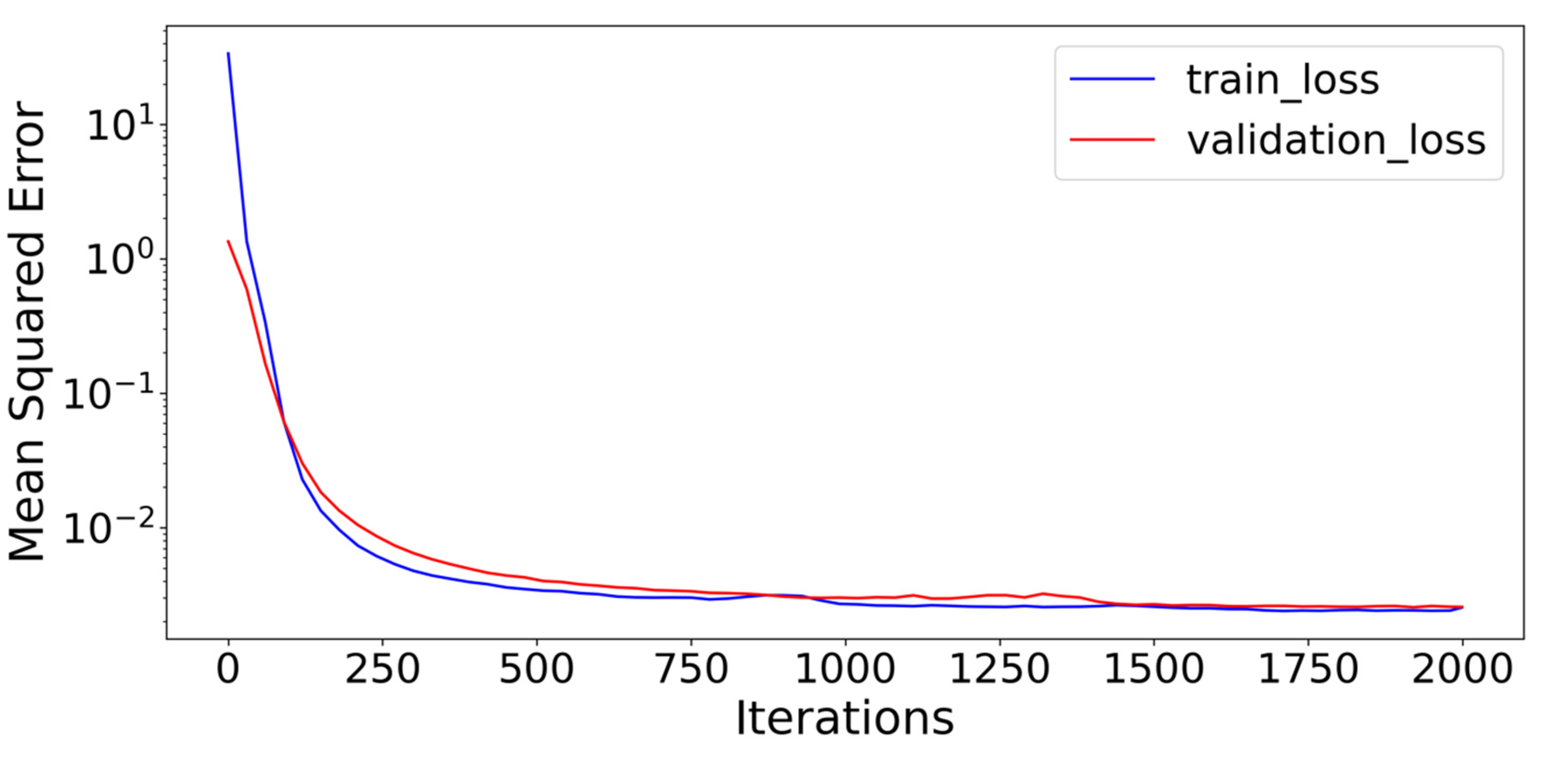
2.4. Training Process
We use both the train and the validation sets in the training process. While the train set is used for the ParFlow-ML model to learn, the validation set is used for providing an unbiased evaluation during training and for avoiding overfitting. ParFlow-ML is evaluated with the validation set every 20 iterations. If the validation loss does not change for the consecutive 200 iterations, the training process will be terminated. The training processes for the Taylor River basin and the Little Washita River basin are similar. Here, we only describe the training process for the Taylor River basin.
For each rainfall–runoff scenario, ParFlow outputs the pressure head and relative saturation at all model layers at each simulation timestep. These model outputs are used as targets for the ML model, and ParFlow’s rainfall information is used as an input. In addition to rainfall information, other ParFlow model input parameters are also used but as static input: topographic slopes, Manning’s roughness values, saturated hydraulic conductivity tensors, and domain’s initial pressure. The static inputs are the same for all rainfall–runoff scenarios.
We configured ParFlow-ML with 8 stacked CausalLSTM layers, each including 1024 nodes. The total number of trainable parameters in ParFlow-ML was approximately 210 million. We choose to train the model for 2000 iterations (for each iteration, the model has to run through the whole training batch of 16 scenarios) initially, then assess the loss. We choose the Adam optimizer [
46] with an initial learning rate of 1 × 10
−3. After 2000 iterations, loss (mean squared error) of the model compared with both the
train and the
validation sets decreased to 2.55 × 10
−3 and 2.57 × 10
−3, respectively (
Figure 5). Since both training and validation losses did not change over the last 200 iterations, we decided to impose early stopping after 2000 iterations.
In the training process, the time for ParFlow-ML to predict one scenario is roughly 5.4 s. Since there are 16 scenarios in the train set, the training batch size is 16. For 2000 iterations, the whole training progress takes around 50 h. All simulations were undertaken in the Princeton Hydrologic Data Center (PHDC), and the training was conducted on NVIDIA A100 GPUs.
2.5. Performance Metrics
Predictions of the pressure head and relative saturation from ParFlow and ParFlow-ML are used to compute streamflow, water table depth (WTD), and total water storage (TWS) and then compared. These three derived variables are evaluated in the
test dataset using four metrics, namely, Spearman’s rho, total absolute relative bias, Kling–Gupta efficiency (KGE [
47,
48]) and the volumetric hit index (VHI [
49]). Spearman’s rho assesses the differences in timing for variables resulting from ParFlow and PredRNN with values closer to one indicating good agreement. The relative bias measures the differences in volume for variables predicted from ParFlow and PredRNN. The KGE coefficient provides an aggregation metric of mean, standard deviation, and correlation between the “simulated” and the “observed” variables. Lastly, the VHI compares the volume of correctly detected simulations with the total volume of correctly detected simulations and missed observations.
3. Results
The test set is used to provide an unbiased assessment of ParFlow-ML. As stated above, the pressure and saturation output from both ParFlow and PredRNN are used to compute streamflow (m3/s), water table depth (m), and total water storage (m3). Below is an evaluation for each of the variables.
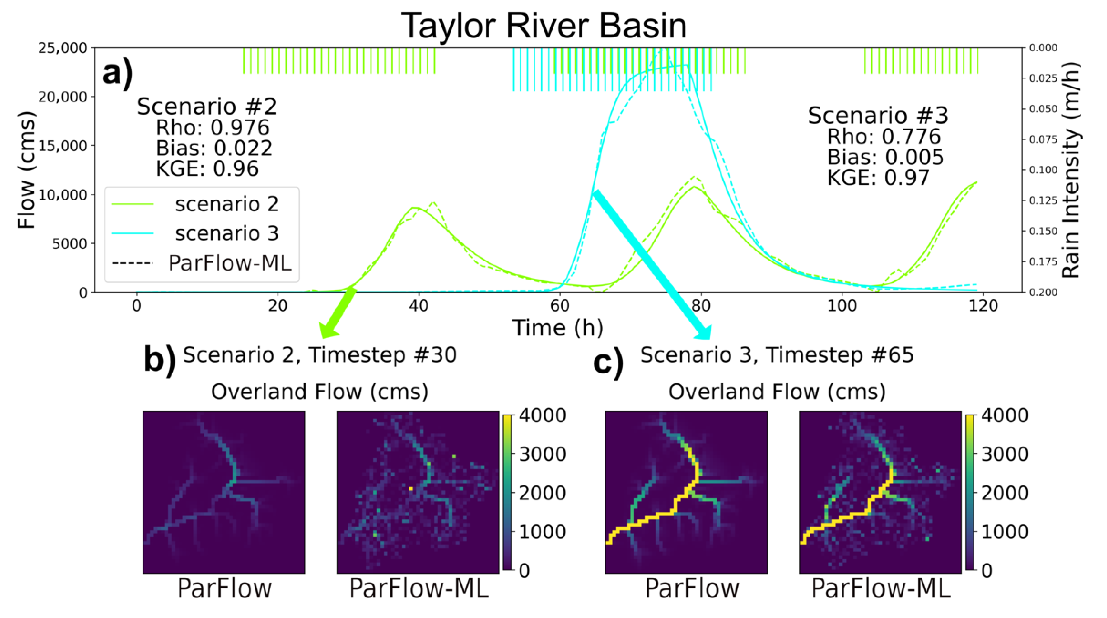
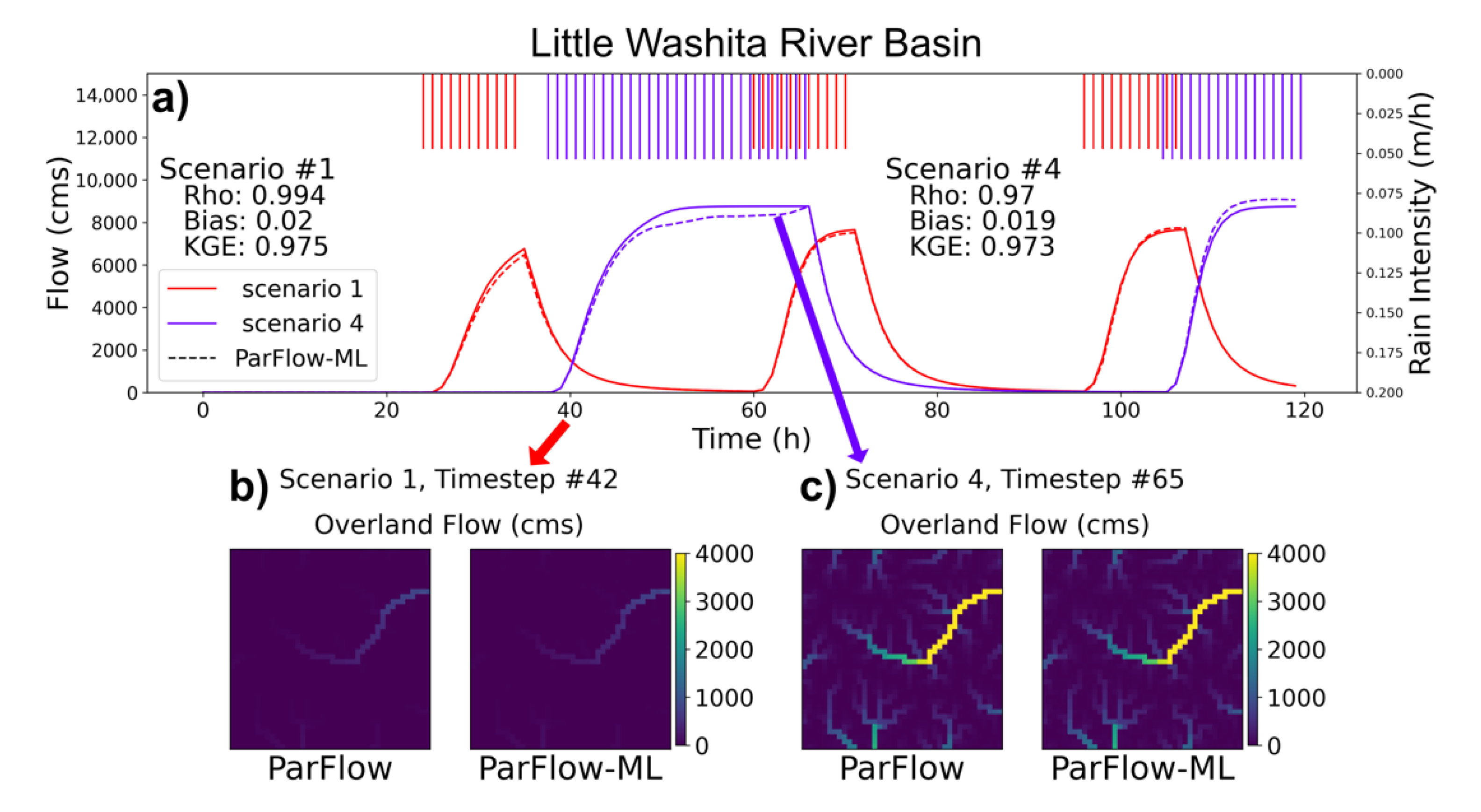
3.1. Streamflow Evaluation
Outflows at gauge locations predicted by ParFlow-ML are evaluated against the ones simulated by ParFlow for all testing scenarios. For the Taylor River basin, the KGE values are 0.747, 0.96, 0.97, and 0.787 for scenarios 21, 22, 23, and 24, respectively (
Table 2). We show two representative testing scenarios, 22 and 23, with different peak times and magnitudes in
Figure 6a. Predicted outflows from ParFlow-ML (dashed lines) closely match (average KGE of 0.97) the ones simulated by ParFlow in both scenarios (
Figure 6a). The ParFlow-ML results compare well with those of ParFlow for the three small rainfall events (scenario 2) and for one large rainfall event (scenario 3).
For the Little Washita River basin, the Spearman’s rho values are 0.994, 0.992, 0.872, and 0.970 for scenarios 21, 22, 23, and 24, respectively (
Table 2). Two representative test scenarios, 21 and 24, with different peak times and magnitudes are shown in
Figure 7a. In scenario 24 (blue lines), ParFlow-ML can predict the peak timing accurately (average Spearman’s rho value of 0.98). However, ParFlow-ML underestimates the first peak and overestimates the second peak.
The spatially distributed outputs of overland flow for baseflow (
Figure 6b and
Figure 7b) and peak flow (
Figure 6c and
Figure 7c) from ParFlow-ML and ParFlow also agree well. ParFlow-ML captures the stream network location and change in magnitude through time, agreeing with the flow routing physics (i.e., flow increases from upstream to downstream cells). Outside of the stream networks, ParFlow-ML exhibits some prediction artifacts and several points where pressure values are predicted as high by ML but as very low in ParFlow. For these locations, ParFlow-ML appears to be predicting a timeseries with a mean close to the predicted values in ParFlow but with much more noise, resulting in pressure fluctuations around a low mean.
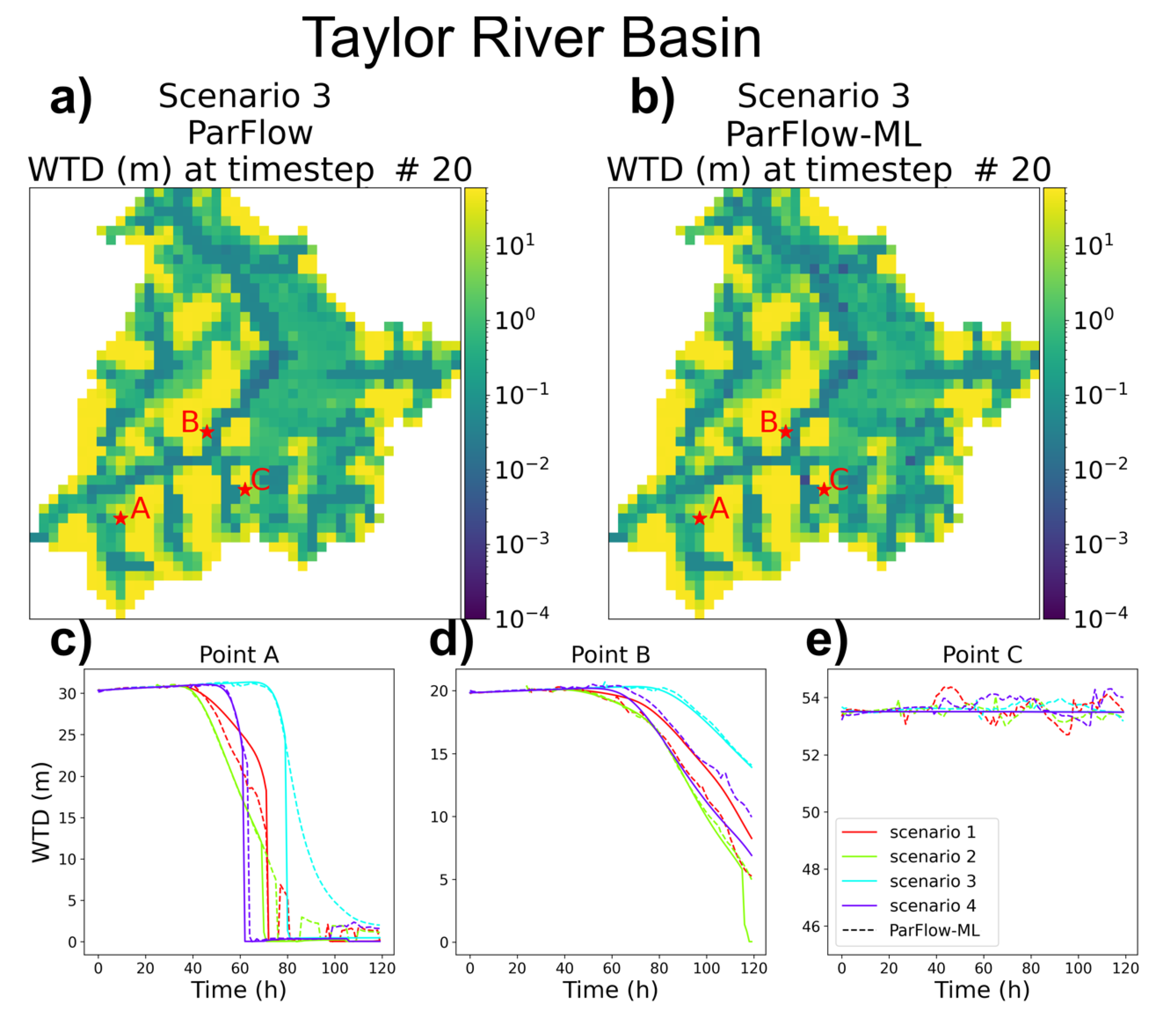
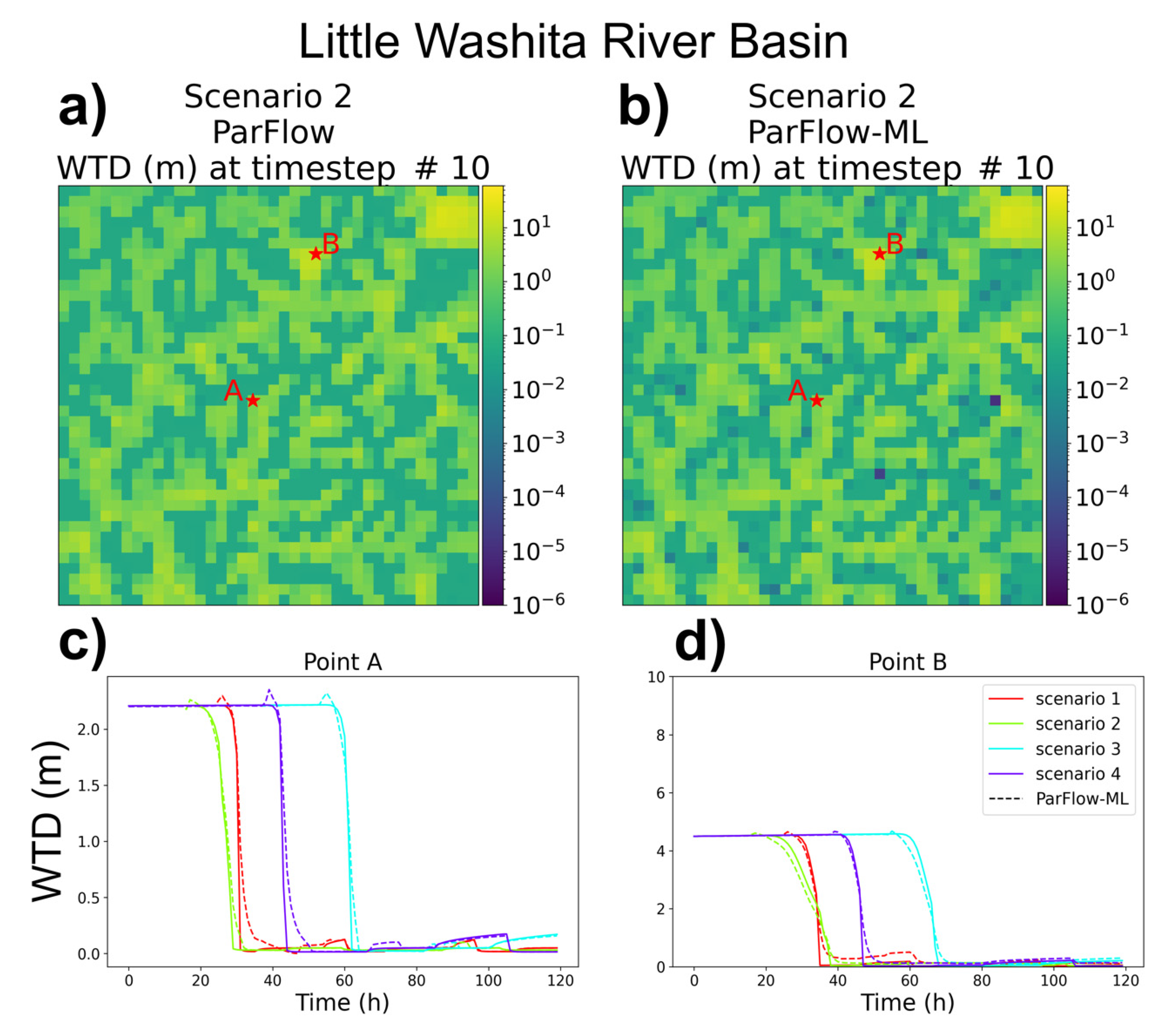
3.2. Water Table Depth (WTD) Evaluation
Figure 8a,b displays the log-scale WTD for scenario 23 at timestep 30. The prediction of river and stream cells (blue cells where the WTD is zero) by ParFlow-ML matches those in ParFlow quite closely. The average VHI over the simulation period for scenarios 21, 22, 23, and 24 are 0.81, 0.84, 0.78, and 0.86, respectively. This is consistent with the stream network comparisons in
Figure 6b,c. Shallower (green; WTD, 0–30 m) and deep (yellow; WTD, >30 m) cells also show similar patterns between ParFlow and ParFlow-ML.
For the WTD timeseries evaluation, over the Taylor River basin, we choose three representative points (shown in
Figure 8 as A, B, and C) to represent the behavior of the stream, shallow, and deep WTD cells, respectively (
Figure 8a,b). Point A starts with a deep WTD, which then decreases rapidly as rain is applied to the domain, becoming overland flow. A decrease in WTD also happens at point B, however, with a smaller magnitude. The WTD at point C remains constant during the simulation period. For points A and B, ParFlow-ML captures the temporal change in WTD for all the scenarios (
Figure 8c,d). For point C, similar behaviors for ParFlow-ML in streamflow prediction can also be seen here with WTD where ParFlow-ML fluctuates around the mean (true) value from ParFlow (
Figure 8e).
We observe a different performance in the Little Washita River domain (
Figure 9), mainly due to the differences in the domain. The Little Washita has a more gentle topography and does not demonstrate the large differences in overall water table depth seen in the more mountainous Taylor River system. The average VHI over the simulation period for scenarios 21, 22, 23, and 24 are 0.85, 0.89, 0.82, and 0.90, respectively. The two points (A, more shallow; B, deeper) chosen in the Little Washita domain both undergo rapid changes as rain is applied, and this behavior is captured well by the ParFlow-ML results.
3.3. Total Water Storage Evaluation
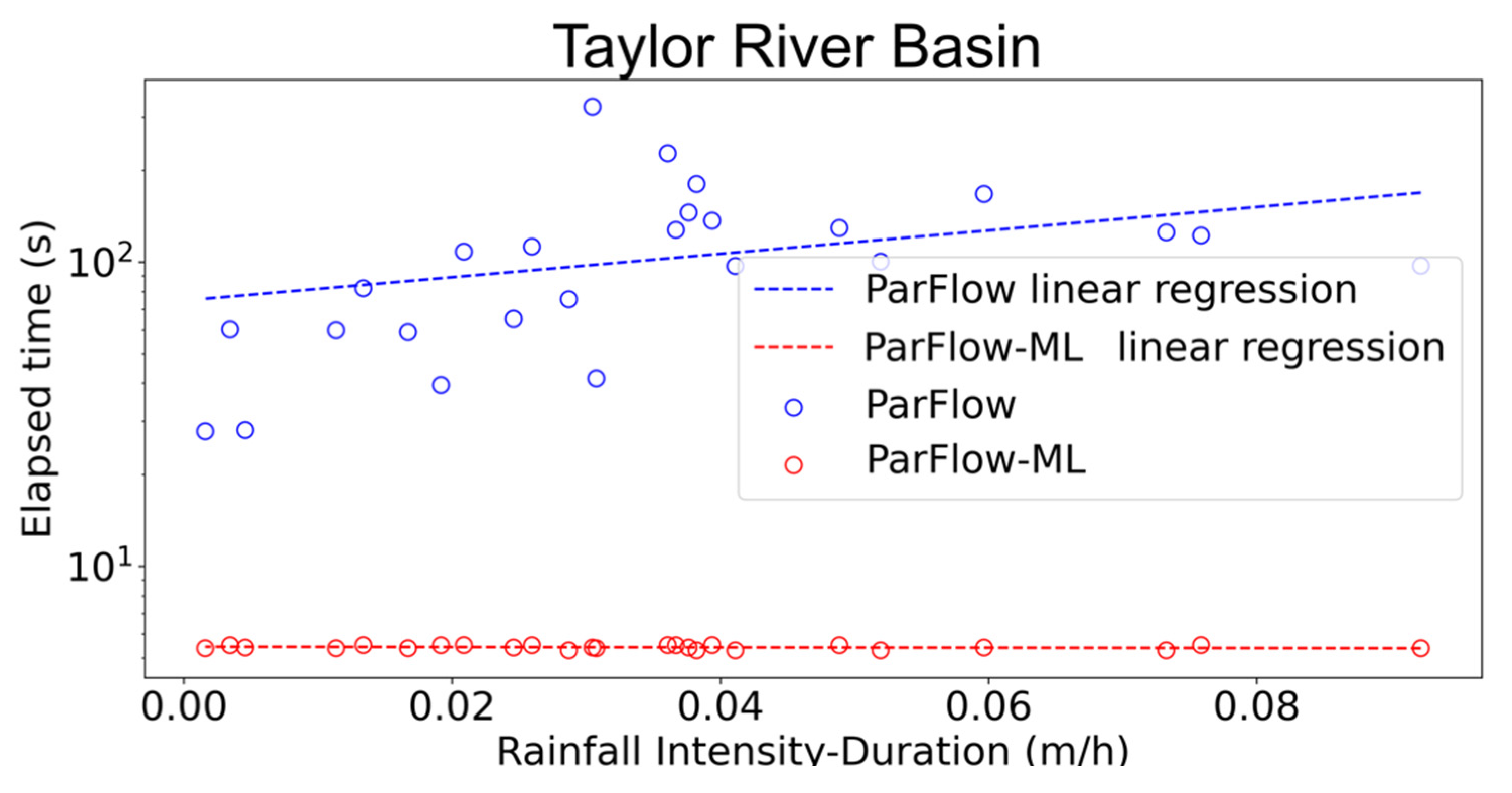
We evaluate the TWS predicted by ParFlow and ParFlow-ML over both simulation domains to evaluate the ability of ParFlow-ML to capture the water balance over the catchment. This is an important evaluation as while the ParFlow model is both globally and locally mass conserving, there is no such intrinsic mass conservation in the ML emulator. Other than being trained on the loss function of total pressure for the given inputs, no external criteria that enforce water balance are imposed. The four
test scenarios (21–24) have different TWSs during the simulation period. While scenarios 21 and 22 in the Taylor River basin show flashier TWS behaviors resulting from shorter rainfall events, TWS changes in scenarios 23 and 24 are slower and exhibit higher magnitudes from longer rainfall events (
Figure 10).
In general, the predicted TWS from ParFlow-ML (dashed lines) respect the overall water balance in both peak time and magnitude with bias values of 0.006, 0.002, 0.001, and 0.003 for scenarios 21, 22, 23, and 24, respectively. The best matching scenarios are 22 and 23 with KGE values of 0.968 and 0.983, respectively. There is only a slight overestimation of TWS in scenarios 21 and 24 during runoff events. The results from the Little Washita test cases (
Figure 11) are similar to those of the Taylor River cases. The four cases performed more similarly, with high Spearman’s Rho and KGE values for both high and low rainfall events.
3.4. Execution Time
An important consideration of an emulation is the reduction in time compared with the original model. We compare the execution times of ParFlow and ParFlow-ML for each of the 24 scenarios in the Taylor River basin. For one scenario prediction, ParFlow uses four CPU cores, while ParFlow-ML uses an A100 GPU.
Since each scenario is characterized by
rain intensity (
I),
rain length (
RL), and
rain frequency (
RecL), for the purposes of execution time comparison, we come up with a combined value,
rainfall intensity-duration (
RID), computed as follows:
As in
Figure 12, the higher the value of RID is, the longer it takes for ParFlow to solve. This is typical for physical hydrologic models as the nonlinear problem becomes more difficult to solve with greater water input necessitating more linear and nonlinear iterations of the solver. We see in this figure, however, that the execution time for ParFlow-ML is independent from RID; it is constant for all the scenarios with a value of 5.4 s. We also see that the execution times are sped up from 5 to 42 times. This is an advantage of the DL models in general and ParFlow-ML since DL treats the hydrological input purely as images.
4. Discussion
In this manuscript, we presented the first emulator of a complex surface–subsurface hydrologic model evaluated over two watersheds. The agreement in prediction from the ParFlow-ML emulator and the original ParFlow hydrologic model is good both spatially and temporally. The temporal behavior is captured by the ParFlow-ML well, with streamflow and water storage peak times predicted by ParFlow-ML matching the output from ParFlow closely for both basins (
Figure 6 and
Figure 7). The average Spearman’s rho values in all the test scenarios for the Taylor River and the Little Washita River basins are 0.909 and 0.957, respectively (
Table 2). The average VHI for the Taylor and the Little Washita River basins are 0.82 and 0.87, respectively. This match in peak timing indicates that ParFlow-ML is able to learn the dynamics of both surface and subsurface water routing correctly. However, there are some biases in streamflow volume and total water storage predicted by ParFlow-ML. The scenario that has the highest streamflow volume or total water storage bias is different between the Taylor and the Little Washita River basins (
Table 2).
Grid cells that have constant values over time are also challenging for ParFlow-ML to predict. ParFlow-ML tends to yield noisy values that fluctuate around the true near-steady values simulated by ParFlow. These near-steady value grid cells do not provide much information for the recurrent module of ParFlow-ML to interpret. However, the magnitudes of these fluctuations are in some cases quite small (
Figure 8).
In general, ParFlow-ML’s predictions are comparable to the ones from ParFlow in both the Taylor River and the Little Washita River basins. The two basins have different sizes, topographies, and land covers, and thus different hydrologic behaviors. The average TWS KGE values of ParFlow-ML for the Taylor River and the Little Washita River basins are 0.931 and 0.957, respectively. ParFlow-ML performs well without imposing mass balance conservation. Beucler et al. [
50] suggesting that applying strict conservations of mass and energy to the machine learning model architecture might reduce the risk of unreliable predictions. By performing well in two different basins, ParFlow-ML shows promise in being transferable to other basins or to larger systems.
The ParFlow simulation time is dependent on the characteristics of the rainfall (
Figure 12). The more intense the rainfall is, the more time it takes for ParFlow to complete a simulation. The ParFlow-ML simulation time is constant and is independent from the rainfall intensity. This enables ParFlow-ML to predict up to 42 times faster than the original ParFlow (
Figure 12).
5. Conclusions
In this study, we discuss the development of an emulator of a complex integrated hydrologic model, ParFlow, based upon the PredRNN deep learning model. By training the ParFlow-ML model on direct inputs and outputs of ParFlow, the emulator was able to predict the evolution of the pressure head and the relative saturation for all grid cells of the model domain over time. We compare the simulation results of ParFlow-ML with those of ParFlow for models of the Taylor River and the Little Washita River basins. Streamflow, water table depth, and total water storage were calculated from the pressure fields for both ParFlow and the emulator.
Spearman’s rho, relative bias, and Kling–Gupta efficiency were used as metrics of comparison. The emulator and ParFlow outputs matched well: the average relative biases of streamflow, water table depth, and total water storage were 0.070, 0.092, and 0.032, respectively. The simulation time of the emulator is up to 42 times smaller than the ones of ParFlow.
While the results are promising, this study still only serves as a proof of concept with synthetic data over two relatively small domains. Nevertheless, this proof of concept demonstrates the ability of an ML emulator that duplicates an entire set of hydrologic model inputs and outputs. This novel study is a step toward constructing larger and more comprehensive ML emulator models that may ultimately ingest meteorological forcing as input and predict land surface states and fluxes in addition to pressure head. Our work provides an additional path to a more efficient hydrologic simulation over large domains at a high resolution.
Author Contributions
Conceptualization, H.T. and R.M.M.; Formal analysis, H.T. and R.M.M.; Funding acquisition, L.E.C. and R.M.M.; Methodology, H.T., E.L., L.D.l.F., R.B.H., P.G., P.M. and R.M.M.; Project administration, L.E.C. and R.M.M.; Software, V.B. and C.C.; Supervision, P.M., L.E.C. and R.M.M.; Validation, H.T., E.L., L.D.l.F. and R.B.H.; Visualization, V.B. and C.C.; Writing—original draft, H.T. and R.M.M.; Writing—review & editing, E.L., L.D.l.F., R.B.H., P.G., L.E.C. and R.M.M. All authors have read and agreed to the published version of the manuscript.
Funding
The HydroGEN convergence accelerator project was funded by US National Science Foundation (NSF) grant CA-2040542 and PG was funded by the LEAP NSF Science and Technology Center.
Institutional Review Board Statement
Not applicable.
Informed Consent Statement
Not applicable.
Data Availability Statement
Acknowledgments
The authors gratefully acknowledge our additional HydroGEN project team members.
Conflicts of Interest
The authors declare no conflict of interest.
References
- Wood, E.F.; Roundy, J.K.; Troy, T.J.; van Beek, L.P.H.; Bierkens, M.F.P.; Blyth, E.; de Roo, A.; Döll, P.; Ek, M.; Famiglietti, J.; et al. Hyperresolution global land surface modeling: Meeting a grand challenge for monitoring Earth’s terrestrial water. Water Resour. Res. 2011, 47. [Google Scholar] [CrossRef]
- Bierkens, M.F.P.; Bell, V.A.; Burek, P.; Chaney, N.; Condon, L.E.; David, C.H.; de Roo, A.; Döll, P.; Drost, N.; Famiglietti, J.S.; et al. Hyper-resolution global hydrological modelling: What is next?: “Everywhere and locally relevant”. Hydrol. Process. 2015, 29, 310–320. [Google Scholar] [CrossRef]
- Burstedde, C.; Fonseca, J.A.; Kollet, S. Enhancing speed and scalability of the ParFlow simulation code. Comput. Geosci. 2018, 22, 347–361. [Google Scholar] [CrossRef][Green Version]
- Kollet, S.J.; Maxwell, R.M.; Woodward, C.S.; Smith, S.; Vanderborght, J.; Vereecken, H.; Simmer, C. Proof of concept of regional scale hydrologic simulations at hydrologic resolution utilizing massively parallel computer resources. Water Resour. Res. 2010, 46, 4201. [Google Scholar] [CrossRef]
- Hokkanen, J.; Kollet, S.; Kraus, J.; Herten, A.; Hrywniak, M.; Pleiter, D. Leveraging HPC accelerator architectures with modern techniques—Hydrologic modeling on GPUs with ParFlow. Comput. Geosci. 2021, 25, 1579–1590. [Google Scholar] [CrossRef]
- Le, P.V.V.; Kumar, P.; Valocchi, A.J.; Dang, H.V. GPU-based high-performance computing for integrated surface-sub-surface flow modeling. Environ. Model. Softw. 2015, 73, 1–13. [Google Scholar] [CrossRef][Green Version]
- Gentine, P.; Pritchard, M.; Rasp, S.; Reinaudi, G.; Yacalis, G. Could Machine Learning Break the Convection Parameterization Deadlock? Geophys. Res. Lett. 2018, 45, 5742–5751. [Google Scholar] [CrossRef]
- Rasp, S.; Pritchard, M.S.; Gentine, P. Deep learning to represent subgrid processes in climate models. Proc. Natl. Acad. Sci. USA 2018, 115, 9684–9689. [Google Scholar] [CrossRef] [PubMed][Green Version]
- Zanna, L.; Brankart, J.M.; Huber, M.; Leroux, S.; Penduff, T.; Williams, P.D. Uncertainty and scale interactions in ocean ensembles: From seasonal forecasts to multidecadal climate predictions. Q. J. R. Meteorol. Soc. 2019, 145, 160–175. [Google Scholar] [CrossRef][Green Version]
- Hsu, K.-L.; Gupta, H.V.; Sorooshian, S. Artificial Neural Network Modeling of the Rainfall-Runoff Process. Water Resour. Res. 1995, 31, 2517–2530. [Google Scholar] [CrossRef]
- Hsu, K.L.; Gupta, H.V.; Gao, X.; Sorooshian, S.; Imam, B. Self-organizing linear output map (SOLO): An artificial neural network suitable for hydrologic modeling and analysis. Water Resour. Res. 2002, 38, 38-1–38-17. [Google Scholar] [CrossRef][Green Version]
- Tao, Y.; Gao, X.; Hsu, K.; Sorooshian, S.; Ihler, A. A deep neural network modeling framework to reduce bias in satellite precipitation products. J. Hydrometeorol. 2016, 17, 931–945. [Google Scholar] [CrossRef]
- Tao, Y.; Gao, X.; Ihler, A.; Sorooshian, S.; Hsu, K. Precipitation identification with bispectral satellite information using deep learning approaches. J. Hydrometeorol. 2017, 18, 1271–1283. [Google Scholar] [CrossRef]
- Wang, C.; Tang, G.; Gentine, P. PrecipGAN: Merging Microwave and Infrared Data for Satellite Precipitation Estimation Using Generative Adversarial Network. Geophys. Res. Lett. 2021, 48, e2020GL092032. [Google Scholar] [CrossRef]
- Fang, K.; Shen, C. Full-flow-regime storage-streamflow correlation patterns provide insights into hydrologic functioning over the continental US. Water Resour. Res. 2017, 53, 8064–8083. [Google Scholar] [CrossRef]
- Feng, D.; Fang, K.; Shen, C. Enhancing Streamflow Forecast and Extracting Insights Using Long-Short Term Memory Networks With Data Integration at Continental Scales. Water Resour. Res. 2020, 56, e2019WR026793. [Google Scholar] [CrossRef]
- Ha, S.; Liu, D.; Mu, L. Prediction of Yangtze River streamflow based on deep learning neural network with El Niño–Southern Oscillation. Sci. Rep. 2021, 11, 11738. [Google Scholar] [CrossRef]
- Kratzert, F.; Klotz, D.; Herrnegger, M.; Sampson, A.K.; Hochreiter, S.; Nearing, G.S. Toward Improved Predictions in Ungauged Basins: Exploiting the Power of Machine Learning. Water Resour. Res. 2019, 55, 11344–11354. [Google Scholar] [CrossRef][Green Version]
- Le, X.H.; Ho, H.V.; Lee, G.; Jung, S. Application of Long Short-Term Memory (LSTM) neural network for flood forecasting. Water 2019, 11, 1387. [Google Scholar] [CrossRef][Green Version]
- Shen, C. A Transdisciplinary Review of Deep Learning Research and Its Relevance for Water Resources Scientists. Water Resour. Res. 2018, 54, 8558–8593. [Google Scholar] [CrossRef]
- Afzaal, H.; Farooque, A.A.; Abbas, F.; Acharya, B.; Esau, T. Groundwater estimation from major physical hydrology components using artificial neural networks and deep learning. Water 2020, 12, 5. [Google Scholar] [CrossRef][Green Version]
- Huang, X.; Gao, L.; Crosbie, R.S.; Zhang, N.; Fu, G.; Doble, R. Groundwater recharge prediction using linear regression, multi-layer perception network, and deep learning. Water 2019, 11, 1879. [Google Scholar] [CrossRef][Green Version]
- Lähivaara, T.; Malehmir, A.; Pasanen, A.; Kärkkäinen, L.; Huttunen, J.M.J.; Hesthaven, J.S. Estimation of groundwater storage from seismic data using deep learning. Geophys. Prospect. 2019, 67, 2115–2126. [Google Scholar] [CrossRef][Green Version]
- Ma, Y.; Montzka, C.; Bayat, B.; Kollet, S. Using Long Short-Term Memory networks to connect water table depth anomalies to precipitation anomalies over Europe. Hydrol. Earth Syst. Sci. 2021, 25, 3555–3575. [Google Scholar] [CrossRef]
- Malakar, P.; Mukherjee, A.; Bhanja, S.N.; Ray, R.K.; Sarkar, S.; Zahid, A. Machine-learning-based regional-scale groundwater level prediction using GRACE. Hydrogeol. J. 2021, 29, 1027–1042. [Google Scholar] [CrossRef]
- Su, Y.; Sen, N.C.F.; Li, W.C.; Lee, I.H.; Lin, C.P. Applying deep learning algorithms to enhance simulations of large-scale groundwater flow in IoTs. Appl. Soft Comput. J. 2020, 92, 106298. [Google Scholar] [CrossRef]
- Pan, B.; Hsu, K.; AghaKouchak, A.; Sorooshian, S. Improving Precipitation Estimation Using Convolutional Neural Network. Water Resour. Res. 2019, 55, 2301–2321. [Google Scholar] [CrossRef][Green Version]
- Vandal, T.; Kodra, E.; Ganguly, S.; Michaelis, A.; Nemani, R.; Ganguly, A.R. DeepSD: Generating high resolution climate change projections through single image super-resolution. In Proceedings of the ACM SIGKDD International Conference on Knowledge Discovery and Data Mining, Halifax, NS, Canada, 13–17 August 2017; pp. 1663–1672. [Google Scholar] [CrossRef]
- Shi, X.; Chen, Z.; Wang, H.; Yeung, D.Y.; Wong, W.K.; Woo, W.C. Convolutional LSTM network: A machine learning approach for precipitation nowcasting. In Proceedings of the 28th International Conference on Neural Information Processing Systems, NIPS’15, Montreal, QC, Canada, 7–12 December 2015; Volume 1, pp. 802–810. [Google Scholar]
- Miao, Q.; Pan, B.; Wang, H.; Hsu, K.; Sorooshian, S. Improving monsoon precipitation prediction using combined convolutional and long short term memory neural network. Water 2019, 11, 977. [Google Scholar] [CrossRef][Green Version]
- Wang, Y.; Gao, Z.; Long, M.; Wang, J.; Yu, P.S. PredRNN++: Towards a Resolution of the Deep-in-Time Dilemma in Spatiotemporal Predictive Learning. In Proceedings of the 35th International Conference on Machine Learning, ICML 2018, Stockholm, Sweden, 15 July 2018; Volume 11, pp. 8122–8131. [Google Scholar]
- Wang, Y.; Wu, H.; Zhang, J.; Gao, Z.; Wang, J.; Yu, P.S.; Long, M. PredRNN: A Recurrent Neural Network for Spatiotemporal Predictive Learning. arXiv 2021, arXiv:2103.09504. [Google Scholar]
- Kuffour, B.N.O.; Engdahl, N.B.; Woodward, C.S.; Condon, L.E.; Kollet, S.; Maxwell, R.M. Simulating Coupled Surface-Subsurface Flows with ParFlow v3.5.0: Capabilities, Applications, and Ongoing Development of an Open-Source, Massively Parallel, Integrated Hydrologic Model. Geosci. Model Dev. 2020, 13, 1373–1397. [Google Scholar] [CrossRef][Green Version]
- Ashby, S.F.; Falgout, R.D. A Parallel Multigrid Preconditioned Conjugate Gradient Algorithm for Groundwater Flow Simulations. Nucl. Sci. Eng. 1996, 124, 145–159. [Google Scholar] [CrossRef]
- Jones, J.E.; Woodward, C.S. Newton-Krylov-Multigrid Solvers for Large-Scale, Highly Heterogeneous, Variably Saturated Flow Problems. Adv. Water Resour. 2001, 24, 763–774. [Google Scholar] [CrossRef][Green Version]
- Kollet, S.J.; Maxwell, R.M. Integrated Surface-Groundwater Flow Modeling: A Free-Surface Overland Flow Boundary Condition in a Parallel Groundwater Flow Model. Adv. Water Resour. 2006, 29, 945–958. [Google Scholar] [CrossRef][Green Version]
- Maxwell, R.M. A Terrain-Following Grid Transform and Preconditioner for Parallel, Large-Scale, Integrated Hydrologic Modeling. Adv. Water Resour. 2013, 53, 109–117. [Google Scholar] [CrossRef]
- Maxwell, R.M.; Condon, L.E.; Kollet, S.J. A High-Resolution Simulation of Groundwater and Surface Water over Most of the Continental US with the Integrated Hydrologic Model ParFlow V3. Geosci. Model Dev. 2015, 8, 923–937. [Google Scholar] [CrossRef][Green Version]
- Richards, L.A. Capillary Conduction of Liquids through Porous Mediums. J. Appl. Phys. 1931, 1, 318–333. [Google Scholar] [CrossRef]
- van Genuchten, M.T. A Closed-Form Equation for Predicting the Hydraulic Conductivity of Unsaturated Soils. Soil Sci. Soc. Am. J. 1980, 44, 892–898. [Google Scholar] [CrossRef][Green Version]
- Srivastava, R.K.; Greff, K.; Schmidhuber, J. Training Very Deep Networks. In NIPS’15, Proceedings of the 28th International Conference on Neural Information Processing Systems, Montreal, QC, Canada, 7–12 December 2015; Neural Information Processing Systems Foundation: Montreal, QC, Canada, 2015; Volume 2, pp. 2377–2385. [Google Scholar]
- Condon, L.E.; Maxwell, R.M. Modified Priority Flood and Global Slope Enforcement Algorithm for Topographic Processing in Physically Based Hydrologic Modeling Applications. Comput. Geosci. 2019, 126, 73–83. [Google Scholar] [CrossRef]
- Schaap, M.G.; Leij, F.J. Database-Related Accuracy and Uncertainty of Pedotransfer Functions. Soil Sci. 1998, 163, 765–779. [Google Scholar] [CrossRef]
- Gleeson, T.; Smith, L.; Moosdorf, N.; Hartmann, J.; Dürr, H.H.; Manning, A.H.; van Beek, L.P.H.; Jellinek, A.M. Mapping Permeability over the Surface of the Earth. Geophys. Res. Lett. 2011, 38. [Google Scholar] [CrossRef][Green Version]
- Maxwell, R.M.; Condon, L.E. Connections between Groundwater Flow and Transpiration Partitioning. Science 2016, 353, 377–380. [Google Scholar] [CrossRef][Green Version]
- Kingma, D.P.; Ba, J.L. Adam: A Method for Stochastic Optimization. In Proceedings of the 3rd International Conference on Learning Representations, ICLR 2015—Conference Track Proceedings, San Diego, CA, USA, 7–9 May 2015. [Google Scholar]
- Gupta, H.V.; Kling, H.; Yilmaz, K.K.; Martinez, G.F. Decomposition of the Mean Squared Error and NSE Performance Criteria: Implications for Improving Hydrological Modelling. J. Hydrol. 2009, 377, 80–91. [Google Scholar] [CrossRef][Green Version]
- Kling, H.; Fuchs, M.; Paulin, M. Runoff Conditions in the Upper Danube Basin under an Ensemble of Climate Change Scenarios. J. Hydrol. 2012, 424–425, 264–277. [Google Scholar] [CrossRef]
- Aghakouchak, A.; Mehran, A. Extended Contingency Table: Performance Metrics for Satellite Observations and Climate Model Simulations. Water Resour. Res. 2013, 49, 7144–7149. [Google Scholar] [CrossRef][Green Version]
- Beucler, T.; Pritchard, M.; Rasp, S.; Ott, J.; Baldi, P.; Gentine, P. Enforcing Analytic Constraints in Neural Networks Emulating Physical Systems. Phys. Rev. Lett. 2021, 126, 098302. [Google Scholar] [CrossRef] [PubMed]
Figure 1.
From Wang et al. [
31], schematic of the causal LSTM, in which the temporal and spatial memories are connected in a cascaded way through gated structures. Colored parts are newly designed operations, concentric circles denote concatenation, and σ is the element-wise Sigmoid function.
Figure 1.
From Wang et al. [
31], schematic of the causal LSTM, in which the temporal and spatial memories are connected in a cascaded way through gated structures. Colored parts are newly designed operations, concentric circles denote concatenation, and σ is the element-wise Sigmoid function.
Figure 2.
From Wang et al. [
31], the final architecture (
top) with the gradient highway unit (
bottom), where concentric circles denote concatenation, and σ is the element-wise Sigmoid function. The blue parts indicate the gradient highway connecting the current timestep directly with previous inputs, while the red parts show the deep transition pathway.
Figure 3.
The Taylor and the Little Washita River basins.
Figure 3.
The Taylor and the Little Washita River basins.
Figure 4.
Rainfall–runoff scenarios in the Taylor River basin for the train (a), validation (b), and test (c) sets. Rain is represented by an upside-down horizontal bar; outflow is represented by a line with a corresponding color.
Figure 4.
Rainfall–runoff scenarios in the Taylor River basin for the train (a), validation (b), and test (c) sets. Rain is represented by an upside-down horizontal bar; outflow is represented by a line with a corresponding color.
Figure 5.
Loss function in the training progress.
Figure 5.
Loss function in the training progress.
Figure 6.
(a) shows the streamflow timeseries at the outlet of the Taylor River basin for ParFlow simulations (solid lines) and ParFlow-ML predictions (dash lines) for scenarios 2 and 3 of the testing set. (b,c) show a snapshot of the stream network of ParFlow simulations (left) and ParFlow-ML predictions (right) for scenario 2 at timestep # 30 (b) and scenario 3 at timestep # 65 (c).
Figure 7.
(a) shows the streamflow timeseries at the outlet of the Little Washita River basin for ParFlow simulations (solid lines) and ParFlow-ML predictions (dash lines) for scenarios 1 and 4 of the testing set. (b,c) show a snapshot of the stream network of ParFlow simulations (left) and ParFlow-ML predictions (right) for scenario 1 at timestep # 42 (b) and scenario 4 at timestep # 65 (c).
Figure 8.
(a) Water table depth from ParFlow simulations for scenario 3 of the testing set at timestep # 20 for the Taylor River basin. (b) Water table depth from ParFlow-ML predictions for scenario 3 of the testing set at timestep # 20 for the Taylor River basin. Locations for three points: A, B, and C are denoted in (a,b). (c) Water table depth from ParFlow simulations (solid lines) and ParFlow-ML predictions (dash lines) for all the scenarios of the testing set at Point A. (d) Water table depth from ParFlow simulations (solid lines) and ParFlow-ML predictions (dash lines) for all the scenarios of the testing set at Point B. (e) Water table depth from ParFlow simulations (solid lines) and ParFlow-ML predictions (dash lines) for all the scenarios of the testing set at Point C.
Figure 9.
(a) Water table depth from ParFlow simulations for scenario 2 of the testing set at timestep # 10 for the Little Washita River basin. (b) Water table depth from ParFlow-ML predictions for scenario 2 of the testing set at timestep # 10 for the Little Washita River basin. Locations for three points: A and B are denoted in (a,b). (c) Water table depth from ParFlow simulations (solid lines) and ParFlow-ML predictions (dash lines) for all the scenarios of the testing set at Point A. (d) Water table depth from ParFlow simulations (solid lines) and ParFlow-ML predictions (dash lines) for all the scenarios of the testing set at Point B.
Figure 10.
Total water storage in the Taylor River basin evaluation between ParFlow simulations (solid lines) and ParFlow-ML predictions (dash lines) for all the scenarios of the testing set.
Figure 10.
Total water storage in the Taylor River basin evaluation between ParFlow simulations (solid lines) and ParFlow-ML predictions (dash lines) for all the scenarios of the testing set.
Figure 11.
Total water storage in the Little Washita River basin evaluation between ParFlow simulations (solid lines) and ParFlow-ML predictions (dash lines) for all the scenarios of the testing set.
Figure 11.
Total water storage in the Little Washita River basin evaluation between ParFlow simulations (solid lines) and ParFlow-ML predictions (dash lines) for all the scenarios of the testing set.
Figure 12.
Execution time comparison between ParFlow simulations (blue points) and ParFlow-ML predictions (red points). Linear regression lines for ParFlow execution time and PredRNN execution time are in blue and red, respectively.
Figure 12.
Execution time comparison between ParFlow simulations (blue points) and ParFlow-ML predictions (red points). Linear regression lines for ParFlow execution time and PredRNN execution time are in blue and red, respectively.
Table 1.
Intensity, length, and recession for the rainfall scenarios. Note that the scenarios are color-coded for train (1–16), validation (17–20), and test (21–24).
Table 1.
Intensity, length, and recession for the rainfall scenarios. Note that the scenarios are color-coded for train (1–16), validation (17–20), and test (21–24).
Scenarios | Rain Intensity (m/h) | Rain Length (h) | Recession Length (h) |
---|
1 | 0.0619 | 14 | 22 |
2 | 0.0557 | 28 | 30 |
3 | 0.0283 | 22 | 17 |
4 | 0.0631 | 7 | 33 |
5 | 0.0334 | 18 | 36 |
6 | 0.0569 | 28 | 21 |
7 | 0.0532 | 21 | 54 |
8 | 0.0119 | 7 | 52 |
9 | 0.0331 | 12 | 35 |
10 | 0.0668 | 29 | 21 |
11 | 0.0344 | 25 | 30 |
12 | 0.0161 | 10 | 47 |
13 | 0.0389 | 16 | 24 |
14 | 0.0775 | 13 | 41 |
15 | 0.0797 | 22 | 57 |
16 | 0.0213 | 12 | 56 |
17 | 0.0677 | 26 | 36 |
18 | 0.0451 | 12 | 15 |
19 | 0.0765 | 13 | 26 |
20 | 0.0792 | 10 | 26 |
21 | 0.0474 | 11 | 25 |
22 | 0.0215 | 28 | 16 |
23 | 0.0357 | 29 | 54 |
24 | 0.0539 | 29 | 38 |
Table 2.
Outflow statistics.
Table 2.
Outflow statistics.
Testing Scenarios | KGE | Relative Bias | Spearman’s Rho |
---|
Taylor | LW | Taylor | LW | Taylor | LW |
---|
21 | 0.747 | 0.975 | 0.177 | 0.020 | 0.947 | 0.994 |
22 | 0.960 | 0.882 | 0.022 | 0.082 | 0.976 | 0.992 |
23 | 0.970 | 0.854 | 0.005 | 0.103 | 0.776 | 0.872 |
24 | 0.787 | 0.973 | 0.135 | 0.019 | 0.937 | 0.970 |
| Publisher’s Note: MDPI stays neutral with regard to jurisdictional claims in published maps and institutional affiliations. |
© 2021 by the authors. Licensee MDPI, Basel, Switzerland. This article is an open access article distributed under the terms and conditions of the Creative Commons Attribution (CC BY) license (https://creativecommons.org/licenses/by/4.0/).