Article

Defining Recovery Potential in River Restoration: A Biological Data-Driven Approach

1
Centre for Agroecology, Water & Resilience, Coventry University, Coventry CV8 3LG, UK
2
Geography and Environment, Loughborough University, Loughborough LE11 3TU, UK
3
River Restoration Centre, Cranfield MK43 0AL, UK
4
Severn Rivers Trust, Martley WR6 6QF, UK
5
Nature Metrics, Egham TW20 9TY, UK
6
College of Agriculture and Environmental Sciences, UNISA, Muckleneuk, Pretoria 0002, South Africa
7
School of Life Sciences, University of Essex, Colchester CO4 3SQ, UK
8
Environment Agency, Bristol BS1 5AH, UK
*
Author to whom correspondence should be addressed.
Water 2021, 13(23), 3339; https://doi.org/10.3390/w13233339
Submission received: 27 October 2021 / Revised: 21 November 2021 / Accepted: 23 November 2021 / Published: 24 November 2021
(This article belongs to the Special Issue River Restoration: Monitoring, Appraisal and Management)

Abstract

:
Scientists and practitioners working on river restoration have made progress on understanding the recovery potential of rivers from geomorphological and engineering perspectives. We now need to build on this work to gain a better understanding of the biological processes involved in river restoration. Environmental policy agendas are focusing on nature recovery, reigniting debates about the use of “natural” reference conditions as benchmarks for ecosystem restoration. We argue that the search for natural or semi-natural analogues to guide restoration planning is inappropriate due to the absence of contemporary reference conditions. With a catchment-scale case study on the invertebrate communities of the Warwickshire Avon, a fifth-order river system in England, we demonstrate an alternative to the reference condition approach. Under our model, recovery potential is quantified based on the gap between observed biodiversity at a site and the biodiversity predicted to occur in that location under alternative management scenarios. We predict that commonly applied restoration measures such as reduced nutrient inputs and the removal of channel resectioning could be detrimental to invertebrate diversity, if applied indiscriminately and without other complementary measures. Instead, our results suggest considerable potential for increases in biodiversity when restoration measures are combined in a way that maximises biodiversity within each water body.

1. Introduction

Through decades of progress by scientists and practitioners, the river restoration community has generated robust understanding of the physical processes involved in successful river restoration. Common “rules-of-thumb” based on stream power and sediment supply [1] and frameworks for river channel design [2] are well established. More recently, detailed engineering guidance has been developed by key advisory bodies, such as the River Restoration Centre in the UK. Whilst these developments have achieved considerable success from an engineering perspective, the biological aspects of river restoration are less well understood. Indeed, many restoration projects fail to result in any detectable improvement in biodiversity despite demonstrably changing the abiotic environment [3,4]. Currently, we lack the ability to predict how biodiversity will respond to a range of alternative river restoration measures targeting hydrology, water quality and physical habitat.
Emerging environmental policy agendas are focusing on nature recovery, reigniting debates about target states and the reference condition concept, which has dominated the practice of biological monitoring for decades [5]. Under the reference condition paradigm, historical examples of ecological communities under least-disturbed conditions are used alongside river typologies to produce an expected community structure for the site in question. The expected community structure is then compared with observed structure to assess the condition of the site and the effectiveness of management measures. Originating from work by British-based scientists in the 1970s, this approach still dominates the practice of freshwater ecosystem assessment worldwide, with prominent examples from Australia [6], Canada [7] and the UK [8]. However, as human activities drive the structure and functioning of ecosystems into new territory—for example, through global climate change, widespread habitat destruction, and species introductions—the past is an increasingly poor guide to the future [9].
We argue that the use of natural or semi-natural analogues to guide restoration planning is ill-conceived due to the absence of contemporary reference conditions and the uncertainties involved in using historical ecological structure to guide target setting. In particular, widespread habitat degradation and fragmentation, species invasions and shifting boundary conditions (e.g., climate) render the reference condition approach inappropriate for restoration planning. Instead, river restoration should be guided by statistical tools that are capable of predicting where restoration will be beneficial for biodiversity, which measures will maximise the benefits, and how species populations will respond. Such capabilities would allow for greater confidence in restoration planning, design and appraisal. By combining long-term biological monitoring records with large-scale environmental data and species distribution modelling, we describe a prototype version of such a tool and demonstrate its application through a case study in a fifth-order catchment characterised by diverse land uses and widespread river modification.

2. Materials and Methods
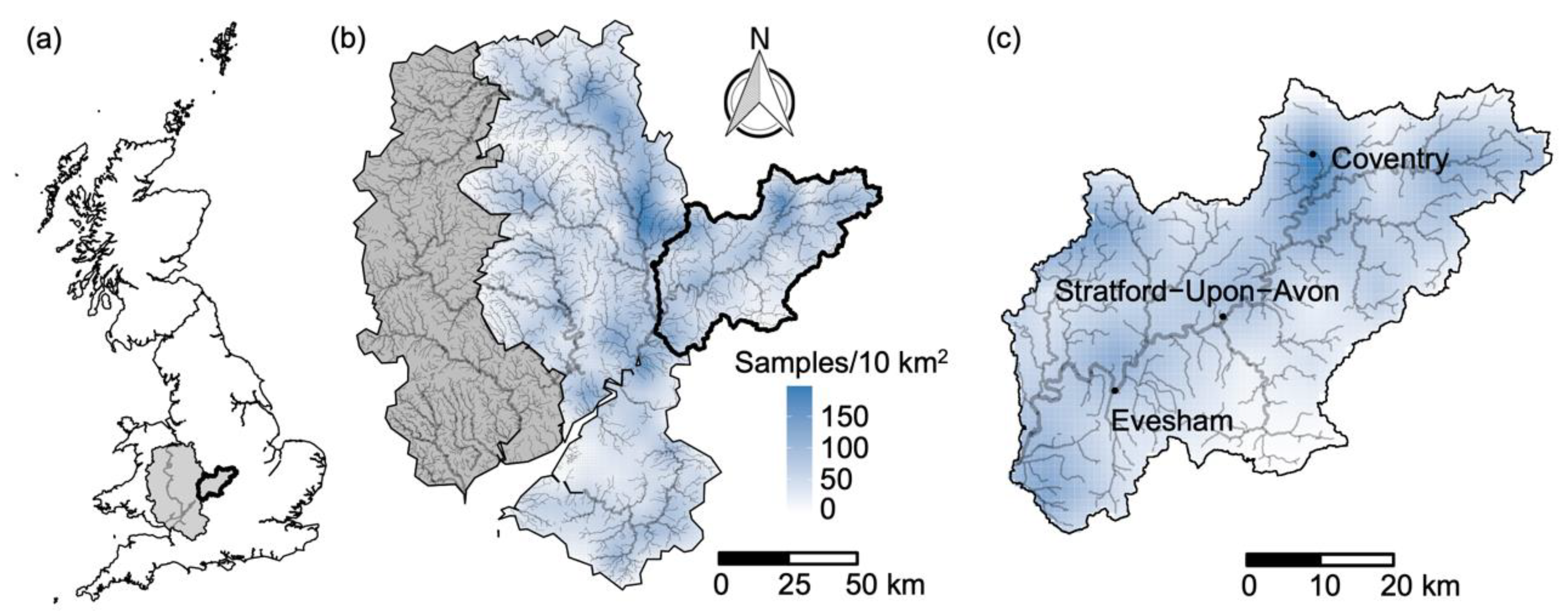
2.1. Study Area

To demonstrate our approach to predicting biodiversity responses after river restoration we selected a relatively data-rich region (England, UK) and taxonomic group (invertebrates). In England, the Environment Agency has collated an extensive river biodiversity dataset, comprising standardised and quality assured invertebrate community data from >100,000 samples since 2002. We limited the modelling domain to the part of the Severn River Basin lying within England (52.19° N, 2.22° W; Figure 1). To ensure that the case study results were tractable for presentation and discussion, we further limited predictions of biodiversity responses to a subset of the modelling domain—the Warwickshire Avon catchment (52.19° N, 1.71° W; Figure 1c).
The River Severn is a sixth-order river with a mean discharge of 107 m3 s−1. The Severn River Basin contains diverse landscapes. Steep slopes, hard rock geology and rough pastures of the Welsh uplands give way to the lowland setting of the English Severn, dominated by a mixture of livestock and arable farming, with sedimentary and alluvial geology. Along with urban and industrial areas, patches of chalk and limestone, and enclaves of semi-natural grassland and woodland, these characteristics make the English Severn representative of lowland landscapes in the UK. Our case study catchment, the Warwickshire Avon, is a fifth-order tributary of the River Severn with a mean discharge of 17.5 m3 s−1 and a total catchment area of 2800 km2. The Avon headwaters include the heavily urbanised and industrial city of Coventry, whilst the lower sections of the river include the historic town of Stratford-Upon-Avon and the intensive horticultural landscape of the Vale of Evesham (Figure 1c).

2.2. Biological Data

We obtained the full river invertebrate monitoring dataset from the Environment Agency’s Fish and Ecology Data Explorer [10]. The full dataset covers the whole of England with sample dates ranging from 1965 to 2019. We used only data collected since 2002 as this was when the Environment Agency adopted more highly standardised sample collection, processing and quality assurance procedures [11]. Despite increased standardisation since 2002, we found that the taxonomic resolution of the data was still highly variable. For example, the same taxon could be described at multiple taxonomic levels, including species, genus, family and higher levels. We therefore aggregated taxon records to the taxonomic levels which retained all, or the vast majority, of the available data, without the need to discard records described at higher levels. We also excluded any records not collected in spring (March–May) and autumn (September–November) as these are the seasons in which the Environment Agency conducts the vast majority of sampling. This data filtering procedure resulted in a total of 8515 samples of invertebrate community structure covering 86 taxa throughout the modelling domain. All taxa were described at family level with the exception of Arachnida, Branchiopoda, Malacostraca and Ostracoda (class), Collembola and Oligochaeta (subclass), Neuroptera (order), and Potamopyrgus (genus). Abundance data were converted to presence-absence for the purposes of modelling taxon occurrence probabilities.

2.3. Environmental Datasets

We gathered a database of environmental variables tied to the Ordnance Survey (OS) Open Rivers network [12] within the modelling domain (Supplementary Figure S1). The database covered a wide range of key river characteristics, from hydrological and geological variables to physical habitat modification, nutrient status and land cover (Table 1). All environmental data were resolved to segments of the river network, with segments defined as reaches between tributaries and other aquatic elements (e.g., lakes, tidal limits). River segments had a mean length of 955 m and an interquartile range of 158–1275 m.
To reflect the magnitude of physical modifications to river channels we obtained the Channel Resectioning Index (CRI) dataset [13]. The CRI dataset contains a series of points quantifying the extent of channel resectioning at 500 m intervals along the 1:50,000 Digital River Network of Great Britain [14] modelled from the UK River Habitat Survey database [15]. We resolved the CRI point data to the OS Open Rivers river network by snapping points to the river with a 500 m threshold snapping distance, and then taking the mean CRI value for each river segment. Where shorter river segments did not intersect with CRI points, which was the case for 3.7% of segments, we took the average of CRI values from segments upstream and downstream.
Table 1. Environmental data sources.
NameShort NameUnitsSource
River network(none)NAOS Open Rivers [12]. Contains OS data © Crown copyright and database right 2021
Channel resectioning indexCRINumber of modificationsModelled from UK River Habitat Survey database [13,15]. © Marc Naura 2016
Log altitudelogaltlog(m)River Invertebrate Classification Tool (RICT) [16]. © Centre for Ecology and Hydrology
Chalk covergchaProportion of upstream catchment
Clay covergcla
Hard rock covergroc
Limestone coverglim
DischargeqcatCategory (1–9)
Longitudinal slopeslopm km−1
P concentration (arable sources)p_aramg L−1Source Apportionment-GIS (SAGIS) [17].
P concentration (livestock sources)p_livmg L−1
P concentration (sewage treatment sources)p_stwmg L−1
P concentration (urban sources)p_urbmg L−1
Water resource availability at Q30cams30Traffic light classificationCatchment Abstraction Management Strategy (CAMS) [18]. © Environment Agency copyright and/or database right 2015
Water resource availability at Q95cams95
Land cover (broadleaved woodland)bwd% coverUK Centre for Ecology and Hydrology Land Cover Maps [19]: 2000 [20]; 2007 [21]; 2015 [22].
Land cover (coniferous woodland)cwd
Land cover (arable)ara
Land cover (improved grassland)igr
Land cover (semi-natural grassland)sgr
Land cover (mountain, heath, bog)hth
Land cover (urban)urb
Basic environmental characteristics of river segments were obtained from the River Invertebrate Classification Tool database [16]. These raster data included altitude, distance from source, log altitude and log area of the upstream catchment, geology cover within the upstream catchment (chalk, clay, hard rock, peat, limestone), discharge category (1–9) and longitudinal slope. From each raster cell intersecting a river segment, we extracted the values of each variable and assigned the mean values to the intersecting segments. The variables describing log altitude of the upstream catchment, distance from source and log area of the upstream catchment were discarded due to strong correlations (ρ ≥ 0.75) with altitude and discharge category. Peat cover in the upstream catchment was also discarded as all river segments had zero values of this variable.
To reflect nutrient status, estimates of orthophosphate concentrations (“P concentrations” from here on) from arable, livestock, sewage treatment and urban sources were obtained from Source Apportionment-GIS (SAGIS) [17]. As an index of stress on each river segment due to water abstraction pressure, we obtained the Catchment Abstraction Management Strategy (CAMS) data [18]. The CAMS data describe water resource availability at different flow percentiles within sub-catchments using a “traffic light” classification. We encoded the data as a factor with four levels: “grey” = 1 (regulated rivers with augmented flows); “green” = 2 (more water than required to meet the needs of the environment); “yellow” = 3 (not enough water left to meet the needs of the environment when all licensed water is abstracted); “red” = 4 (actual water levels below what is required to meet the needs of the environment). From the CAMS database we extracted only variables pertaining to Q30 and Q95 as indicators of water resource availability at relatively high and low discharges respectively. Both SAGIS and CAMS datasets were in polygon format at the water body level (defined under UK legislation as a discrete and significant element of surface water). We resolved estimates of P concentrations and CAMS variables to the river network by extracting values from polygons which intersected with each river segment.
Riparian land cover within 1 km of the river network was represented using the Centre for Ecology and Hydrology Land Cover Maps series (percentage aggregate class raster data at 1 km resolution) [19]. To obtain an annual time series of land cover for each 1 km raster cell along the river network, we first fitted linear models of the percentage cover of each aggregate class from the 2000 [20], 2007 [21] and 2015 [22] land cover maps, then predicted the percentage cover for each year before extracting mean values along each river segment and standardising to 100% total land cover.

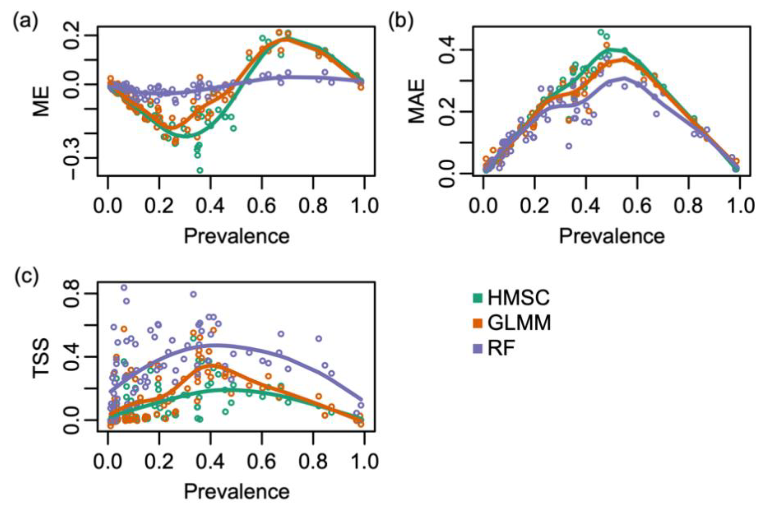
2.4. Species Distribution Modelling

To drive predictions of biodiversity responses to river restoration we fitted a range of species distribution models (SDMs) and compared their predictive performance. Candidate models were initially identified based on a previous assessment recommending that future studies fit a set of four best-performing models and evaluate their relative performance for the specific application [23]. Of the four best-performing models, we were unable to fit the Species Archetype Model (SAM) [24] as the software to do so was no longer available. Neither was it practically possible to fit the multi-taxon Hierarchical Modelling of Species Communities (HMSC) model [25] due to the computationally intensive nature of the method and the large volume of data involved. Instead, we fitted taxon-by-taxon HMSC models with spatial random effects, and generalized linear mixed effects models (GLMMs; probit link) without interactions between independent variables. The decision to omit interactions from GLMMs was made on the basis that we had a relatively large number of environmental predictors and no a priori knowledge of interactions between them, in contrast to the smaller sets of predictors used in previous assessments [23]. In the GLMMs and HMSC models, we included year as a random effect to account for temporal pseudoreplication [26] and season (spring, autumn) as a fixed effect to account for seasonal variation. In addition to these two recommended methods, we also fitted Random Forests (RF) models as the RF method may perform better than others when faced with a relatively large number of potentially interacting predictors [27], as was the case in our study. Season and year were included as predictors in RF models. All models were fitted on a taxon-by-taxon basis and biodiversity responses assessed by stacking predictions for each taxon.
For model fitting and evaluation purposes, all models were trained on the same subset (75%) of data and predictive performance evaluated using the remaining data (25%). HMSC models were fitted using the sampleMcmc function from the Hmsc package in R [28] with a burn-in of 500, no thinning and 250 samples from each of two chains. We checked convergence of HMSC models by ensuring that effective sample sizes were >10% of the theoretical sample size, and chain mixing by ensuring that all potential scale reduction factors were <1.1. GLMMs were fitted using the glmer function from the lme4 package in R [29]. RF models were fitted using the ranger function from the ranger package in R [30] with the Gini index as the impurity measure and the keep.inbag argument set to TRUE. Predictive performance was evaluated using mean error (ME), mean absolute error (MAE), and the true skill statistic (TSS). To facilitate comparisons between models, we fitted generalized additive models (gam function from the mgcv package in R) [31] with a smooth term on taxon prevalence (proportion of samples in which the taxon occurred) to each model type and evaluation metric.

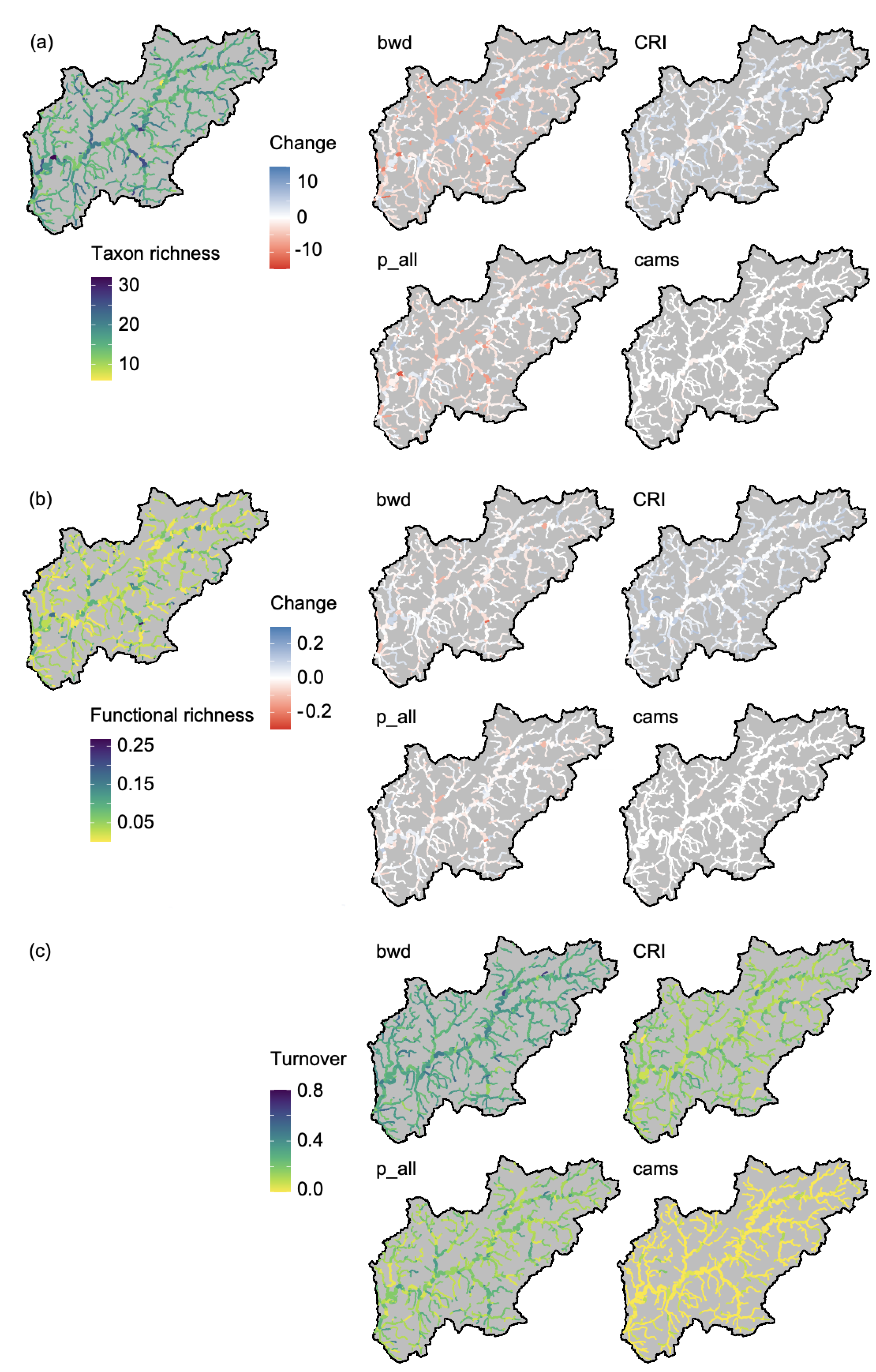
2.5. Restoration Scenarios

Using the best performing SDM method, we predicted biodiversity responses to a range of restoration scenarios (Table 2). Rather than attempting to produce an exhaustive set of restoration scenarios, we focused only on scenarios which could be quantitatively represented using the most well-established datasets available to us for this prototype model. We constructed two sets of scenarios. A set of four high-level restoration measures was used to examine predicted biodiversity responses in detail. This high-level set included individual measures of riparian woodland creation (“bwd” in Table 2), removal of channel resectioning (“CRI”), reduction of P concentrations from all sources by 50% (“p_all”) and abstraction relicensing to bring all water resource availability classifications to “green” status (“cams”). Another set of eight lower-level restoration measures was used to estimate recovery potential among water bodies, as well as predicting the combination of restoration measures which would maximise biodiversity benefits within each water body. This larger set of measures included reduction of P concentrations from individual sources, and abstraction relicensing to bring all water resource availability classifications to “green” status separately at higher flows (Q30) and lower flows (Q95), as well as riparian woodland creation and removal of channel resectioning (Table 2).
For each restoration measure, or combination of measures, predictions were made for the whole river network within the case study catchment by modifying the environmental attributes of each river segment. Predictions were produced for each year (2002–2019) and two seasons (spring, autumn) and then averaged across all years and both seasons to reflect long-term means of species occurrence probabilities. The same averages across years and seasons were also calculated using the baseline environmental attributes of the river network. We indexed biodiversity responses per river segment using taxon richness, functional richness, and turnover (Jaccard dissimilarity; a measure of change in community composition following restoration), and for the whole catchment using beta diversity (a measure of spatial variability in community composition), gamma diversity (number of taxa present within the whole catchment) and change in mean occurrence probability for each taxon, compared to the baseline. Functional richness was calculated using the dbFD function from the FD package in R [32] as a standardised value between 0 (no traits present) to 1 (all possible traits present). Traits describing body size, resistance forms and diet [33] were used in the calculation of functional richness as these traits are most informative for large-scale biodiversity modelling [34] and correspond to the axes of generalised life history models for river ecosystems [35].
Recovery potential was quantified for all water bodies in which any measure, or combination of measures, was predicted to result in increases in both taxon richness and functional richness. For these water bodies, we identified the measure(s) predicted to result in the greatest stream length-weighted mean taxon richness gains across all river segments within the water body. We then ranked waterbodies in ascending order by the maximum predicted taxon richness gain under the model. This process was repeated separately for functional richness. Ranks for taxon richness and functional richness were averaged for each water body and then standardised across the whole river network to values between 1 (highest predicted increases) and 0 (lowest predicted increases). The resulting value was taken as a measure of relative recovery potential among water bodies. Finally, recovery potential was modelled as a function of environmental variables using linear regression (lm function in R) [36] to explore explanations for predicted patterns, after logit transforming the response variable. We explored linear models of recovery potential with additive effects and all possible two-way interactions.

3. Results

SDM evaluations showed that, of the three candidate models, RF models performed best (Figure 2). GLMMs and HMSC models overpredicted the occurrence of moderately rare taxa and underpredicted the occurrence of moderately common taxa. RF models had the lowest mean absolute errors and the highest TSS values across the entire range of taxon prevalence. However, TSS values for RF models were highly variable for rarer taxa, with overall ranges of −0.01 to 0.84.
Under the four high-level restoration scenarios, only the CRI scenario was predicted to result in mean increases in taxon richness and functional richness across the case study catchment (Figure 3). The bwd (riparian woodland creation) and p_all (50% P reduction) scenarios were predicted to result in slight decreases in mean richness measures, with several river segments predicted to lose >10 taxa and >20% of their functional richness (Figure 3a,b and Figure 4). Predicted beta diversity changes were less pronounced, with slight average gains under the bwd scenario and mean decreases under p_all (Figure 3c). The bwd scenario was also associated with the highest rates of turnover (predicted change in community composition following restoration; Figure 3d), whereas the cams scenario had relatively little effect on any biodiversity indices.
Gamma diversity decreases under bwd and p_all were predicted to equate to the loss of 15 taxa from the catchment, whilst gamma diversity predictions for the CRI scenario (removal of channel resectioning) were also negative (Figure 3e). In line with these results, most taxa were predicted to undergo slight decreases in mean occurrence probability (Figure 3f). However, stronger decreases were predicted under bwd for two molluscan taxa (Hydrobiidae, Planorbidae) and stronger increases under bwd and CRI for three insect families (Ephemeridae, Polycentropodidae, Sericostomatidae). These predicted changes were distributed throughout the river network with no clear spatial pattern in terms of stream order or sub-catchment (Figure 4).
Under the eight lower-level restoration measures, all water bodies had at least one combination of measures that was predicted to increase mean taxon richness and functional richness (Figure 5a). The number of restoration measures required to maximise increases in taxon richness (Figure 5b) and functional richness (Figure 5c) ranged from a single measure to a combination of four measures. The CRI measure was most commonly involved in the set of measures predicted to maximise increases in taxon richness (Figure 5d) and functional richness (Figure 5e). Taxon richness along 100% of the total 1380 km stream length was predicted to benefit to some degree from the removal of channel resectioning, whereas for functional richness 1352 km (98%) of stream length was predicted to respond positively to this measure. The bwd and p_urb (50% P reductions from urban sources) measures were also involved in predicted increases in taxon richness across 29% of the total stream length, and increases in functional richness across >50% of the total stream length. By contrast, the cams95 measure was predicted to benefit biodiversity along <5% of the stream length, whereas the cams30 measure was not predicted to benefit biodiversity anywhere within the case study catchment. Figure 6 shows where each lower-level restoration measure contributed to recovery potential throughout the catchment. In general, increases in taxon richness and functional richness were predicted to occur in unison, albeit with considerable variation and a levelling-off of functional richness increases at higher taxon richness increases (Figure 5f).
In terms of explaining the recovery potential of river segments, regression models with two-way interactions [F152, 585 = 4.11, p < 0.0001, R2 = 0.39] and without interactions [F17, 721 = 6.74, p < 0.0001, R2 = 0.12] were both significant (Supplementary Tables S1 and S2). Under the model without interactions, CRI, gcha, p_urb and cams30 were significant positive predictors of recovery potential, whereas logalt and p_stw were significant negative predictors. Under the more complex regression model, several interactions were significant. These involved a set of interactions between CRI, discharge category (qcat) and slope (slop), and two other sets of interactions among gcha, P concentrations (p_liv, p_stw, p_urb) and cams95, and between p_urb and several land cover classes (Supplementary Table S2).

4. Discussion

Overall, our results indicate that commonly applied restoration measures such as riparian tree planting, reduced nutrient inputs and the removal of channel resectioning could be detrimental to catchment-scale invertebrate biodiversity if applied indiscriminately and without other complementary measures. On the other hand, we indicate considerable potential for catchment-wide increases in biodiversity when restoration measures are applied in combinations adapted to baseline environmental conditions and ecological communities.

4.1. Implications for River Restoration Planning

Our findings suggest that careful spatial planning is necessary to maximise positive outcomes and avoid negative biodiversity outcomes in river restoration. Much of the river network within the case study catchment was predicted to experience declines in invertebrate biodiversity under four high-level restoration measures when these measures are applied in isolation. In particular, the establishment of 100% broadleaved woodland within 1 km of the whole river network (scenario “bwd”) was predicted to result in considerable declines in the distributions of several taxa and the extinction of 15 taxa from the catchment (Figure 3). The taxa predicted to suffer the greatest declines under this scenario included those considered relatively pollution tolerant (e.g., Planorbidae, Hydrobiidae, Glossiphoniidae) as well as insect families considered more sensitive (Hydropsychidae, Glossosomatidae, Leptoceridae). Whilst it is unlikely that the conversion of all riparian areas to woodland could be achieved in reality, particularly in urban areas, this finding adds further weight to growing evidence that indiscriminate tree planting may not be an effective strategy for large-scale biodiversity conservation [37].
The removal of all elements of channel resectioning (“CRI”), such as reinforced beds and banks—a commonly targeted measure in river restoration—was predicted to increase alpha diversity on average. However, applied indiscriminately and in isolation, this restoration strategy was also predicted to decrease gamma (catchment-scale) diversity through small but significant impacts on populations of Arachnida, the insects Calopterygidae and Ceratopogonidae, and the gastropods Physidae and Valvatidae. The reduction of P concentrations from all sources by 50% (“p_all”)—a measure often targeted by agri-environment schemes and water company strategies—was predicted to lead to a mean decline in all measures of invertebrate biodiversity. On the other hand, abstraction relicensing efforts to bring the whole river network into “green” water resource availability status at both high and low flows (“cams”) was predicted to have little effect on any invertebrate biodiversity measure.
With regards to agri-environment schemes, our findings can inform implementation of new Environmental Land Management Schemes (ELMS) in the UK. With the phasing out of the Common Agricultural Policy’s Basic Payment Scheme by 2024, ELMS enacts the UK government’s 25-Year Environment Plan and the Agriculture Bill to fund land managers for services that provide ‘public-good’. This includes actions that support local nature recovery and landscape recovery. To be effective in achieving these aims, ELMS should target the measures predicted to be most beneficial for biodiversity, and the locations with the greatest recovery potential.
When restoration measures are applied in combinations designed specifically for each water body, our results suggest that considerable catchment-wide gains in invertebrate biodiversity can be achieved. The most effective combination of measures typically included the removal of channel resectioning (“CRI”) along with riparian woodland creation (“bwd”) and a 50% reduction in P concentrations from urban sources (“p_urb”) (Figure 5d,e and Figure 6). These and other measures were predicted to contribute to increases in both taxonomic and functional measures of invertebrate biodiversity, suggesting that river restoration can be designed to improve functional outcomes (e.g., resistance, resilience, trophic diversity) as well as structural outcomes. However, the number of measures required to maximise functional richness gains (Figure 5c) was typically greater than the number required to maximise taxon richness gains (Figure 5b). Furthermore, the relationship between predicted taxon richness and functional richness gains (Figure 5f) corroborates previous suggestions that functional outcomes are more challenging to achieve than taxonomic outcomes [38]. This is due to functional redundancy in the taxa predicted to colonise a newly restored site.
We found no clear spatial structure in recovery potential, suggesting that restoration strategies cannot focus on particular water bodies or discrete areas with specific baseline environmental conditions (e.g., urban areas). In our case study, areas with high recovery potential (i.e., >0.75) could be found throughout the catchment. However, regression models explaining recovery potential did indicate several relationships that could help guide river restoration planning. Firstly, and unsurprisingly, locations with a greater degree of channel resectioning and higher P concentrations from urban sources had greater recovery potential. Secondly, less obvious relationships were found indicating that chalk geology and water bodies with lower water resource availability (e.g., “yellow” and “red” classifications under CAMS) [18] may also be associated with greater recovery potential, whereas locations with higher P concentrations from sewage treatment works were strongly associated with lower recovery potential. Significant interactions among the channel resectioning index (CRI), discharge category, slope, P concentrations and land use suggest that recovery potential is a complex emergent feature of the modelling and prediction procedure. Indeed, the SDM method selected on the basis of its comparatively strong predictive performance, random forests, is particularly well suited to reflect complex, high-order and nonlinear interactions between predictors. Our prototype model for quantifying recovery potential represents a guide for restoration planning in light of these complexities. However, SDM evaluation metrics (Figure 2) indicate that there is considerable room for improvement.

4.2. Limitations and Further Research

Further development of the prototype should involve work on several fronts to improve model predictions. Firstly, future work should compare the performance of a wider range of SDM methods, fitted using alternative sets of environmental predictors under a stricter evaluation regime (e.g., k-fold cross validation). In doing so, the modelling domain should be expanded to include higher volumes of monitoring data. In the UK, for example, integration of freshwater biological monitoring datasets from the devolved nations of England, Scotland and Wales would offer potential for greatly enhanced evidence-based management of river ecosystems. Further development should involve integrating spatial datasets reflecting a wider range of stressors, such as pesticide concentrations and riverine barrier (e.g., dams, weirs) densities, subject to data availability at an appropriate scale and resolution. The incorporation of future climate projections, for example on hydrological variability and thermal extremes, would also make a critical contribution to ensure that climate risk is captured in the model.
Secondly, future modelling studies should look to integrate more ecological theory. In particular, the present approach represents a poor integration of the metacommunity framework, which has previously been suggested as central to understanding the success and failure of river restoration from an ecological perspective [39]. The metacommunity concept states that observed species distributions may not reflect underlying abiotic conditions due to dispersal processes that prevent access to suitable habitat patches (patch dynamics) or increase access to unsuitable habitat patches (mass effects), as well as neutral processes which are independent of the abiotic environment [40]. Our approach to mitigating confounding effects due to dispersal limitation was to confine modelling to a single river basin (i.e., the Severn Basin) on the assumption that, at least in the medium-term (5–10 years), all taxa would have access to restored habitats throughout the modelling domain. However, even within a single river basin, dispersal constraints could limit biodiversity responses to restoration. On the other hand, the inclusion of data from larger modelling domains (e.g., the whole of Europe) could increase our capacity to predict positive outcomes and even model the risk of species invasions under alternative restoration and climate change scenarios.
In addition, future models should be improved by integrating background knowledge on phylogeny and species traits, and by representing spatial structure in the data. Such background knowledge can be used in hierarchical models to explain variation in species niches, whilst the inclusion of spatial random effects structures can better reflect metacommunity processes. Although HMSC does offer such capabilities in multi-taxon species distribution modelling [25], computational demands mean that it is not currently feasible to apply the multi-taxon version across the largest datasets. Future progress in this area could hinge on advances in high-performance computing, as well as greater integration of ecological theory in biodiversity models.
A third area for improvement relates to the taxonomic level at which we characterised invertebrate communities. The aggregation of taxa mostly to family and higher levels was a pragmatic response to the variety of taxonomic levels recorded in the source data. Environment Agency monitoring data have increasingly been recorded at species level for the majority of taxonomic groups. However, many individual specimens are still recorded at a range of levels, from class to species, due to challenges with identifying all specimens to finer taxonomic resolutions. If records at higher levels (e.g., genus and higher) are excluded, this runs the risk of introducing uncertainty into the estimation of taxon distributions. DNA-based methods may render this problem obsolete in the future by resolving communities to species or even haplotype level, yet there is still a need to leverage the value of historical data collected using traditional, manual techniques. Thus, a priority for data-driven biodiversity modelling is to work at finer taxonomic resolutions. This could be achieved by explicitly representing the probability that each taxon belongs to any other higher taxonomic group recorded in the dataset. In a similar vein, biodiversity scientists should develop models capable of integrating historical monitoring datasets with new observations generated using DNA metabarcoding, in order to harness the power of both historical monitoring and molecular technologies. To date, we are not aware of any established approaches for dealing with these issues.

5. Conclusions

Until now, the river restoration community has largely concentrated efforts on developing the geomorphological and engineering aspects of its practices. A shift towards greater integration of ecology in river restoration is being hindered by limited understanding of biological recovery potential. With further development, our model to quantify recovery potential in river networks can help to inform spatial planning, design and appraisal of river restoration projects. Our case study suggested that coordinated efforts to deliver a range of restoration measures in different parts of the catchment could yield considerable biodiversity increases. On the other hand, indiscriminate applications of single restoration measures in isolation could have detrimental effects on biodiversity at the catchment scale. The combination of measures most commonly predicted to yield biodiversity increases in our case study was the removal of channel resectioning plus riparian woodland creation and/or reductions in nutrient concentrations from urban sources. We encourage river managers to plan restoration activities at the catchment scale whilst recognising that, from a biodiversity perspective, the most effective combination of measures depends on local baseline conditions.

Supplementary Materials

The following are available online at https://www.mdpi.com/article/10.3390/w13233339/s1, Figure S1: Environmental variables used for modelling recovery potential in the Warwickshire Avon case study catchment, Table S1: Summary statistics for the linear model predicting recovery potential as a function of environmental variables without interactions, Table S2: Summary statistics for the linear model predicting recovery potential as a function of environmental variables with all possible two-way interactions.

Author Contributions

Conceptualization, M.A.W., C.L., T.L., J.E., M.M. (Mike Morris) and M.V.D.W.; Methodology, M.A.W., M.M. (Morwenna Mckenzie), M.N., L.A., A.J.D. and A.B.; Formal Analysis, M.A.W.; Data Curation, M.A.W. and M.M. (Morwenna Mckenzie); Writing—Original Draft Preparation, M.A.W.; Writing—Review and Editing, M.M. (Morwenna Mckenzie), M.N., L.A., M.M. (Mike Morris), M.V.D.W., A.J.D., A.B., C.L., T.L. and J.E.; Visualisation, M.A.W. The views expressed are those of the authors and not necessarily those of their organisation. All authors have read and agreed to the published version of the manuscript.

Funding

This work received support from Severn Rivers Trust and Coventry University under a match-funded PhD studentship agreement.

Institutional Review Board Statement

No human or animal was involved with this study and hence ethics approval was not needed.

Data Availability Statement

With the exception of basic data on river environments and the channel resectioning index, all data used in this study are openly available from sources quoted in the text. Basic data on river environments from the River Invertebrate Classification Tool may be requested from the UK Centre for Ecology and Hydrology. Channel resectioning index data may be made available by the data owner (M.N.).

Conflicts of Interest

The authors declare no conflict of interest.

References

  1. Brookes, A. Recovery and restoration of some engineered British river channels. In River Conservation and Management; Boon, P.J., Calow, P., Petts, G.E., Eds.; Wiley: Chichester, UK, 1992; pp. 337–352. [Google Scholar]
  2. Rosgen, D.L. Applied River Morphology; Wildland Hydrology: Pagosa Springs, CO, USA, 1996. [Google Scholar]
  3. Hering, D.; Aroviita, J.; Baattrup-Pedersen, A.; Brabec, K.; Buijse, T.; Ecke, F.; Friberg, N.; Gielczewski, M.; Januschke, K.; Köhler, J.; et al. Contrasting the roles of section length and instream habitat enhancement for river restoration success: A field study of 20 European restoration projects. J. Appl. Ecol. 2015, 52, 1518–1527. [Google Scholar] [CrossRef]
  4. Verdonschot, R.C.; Kail, J.; McKie, B.G.; Verdonschot, P.F. The role of benthic microhabitats in determining the effects of hydromorphological river restoration on macroinvertebrates. Hydrobiologia 2016, 769, 55–66. [Google Scholar] [CrossRef] [Green Version]
  5. Wright, J.F.; Moss, D.; Armitage, P.D.; Furse, M.T. A preliminary classification of running-water sites in Great Britain based on macroinvertebrate species and the prediction of community type using environmental data. Freshw. Biol. 1984, 14, 221–256. [Google Scholar] [CrossRef]
  6. Davies, P.E. Development of a national river bioassessment system (AUSRIVAS). In Assessing the Biological Quality of Freshwaters: RIVPACS and Other Techniques; Wright, J.F., Sutcliffe, D.W., Furse, M.T., Eds.; Freshwater Biological Association: Ambleside, UK, 2000; pp. 113–124. [Google Scholar]
  7. Metcalfe, R.A.; Mackereth, R.W.; Grantham, B.; Jones, N.; Pyrce, R.S.; Haxton, T.; Luce, J.J.; Stainton, R. Aquatic Ecosystem Assessments for Rivers; Ministry of Natural Resources: Peterborough, ON, Canada, 2013.
  8. Clarke, R.T.; Wright, J.F.; Furse, M.T. RIVPACS models for predicting the expected macroinvertebrate fauna and assessing the ecological quality of rivers. Ecol. Model. 2003, 160, 219–233. [Google Scholar] [CrossRef]
  9. Tonkin, J.D.; Poff, N.L.; Bond, N.R.; Horne, A.; Merritt, D.M.; Reynolds, L.V.; Olden, J.D.; Ruhi, A.; Lytle, D.A. Prepare river ecosystems for an uncertain future. Nature 2019, 570, 301–303. [Google Scholar] [CrossRef]
  10. Environment Agency Ecology & Fish Data Explorer. Available online: https://environment.data.gov.uk/ecology/explorer/ (accessed on 19 October 2021).
  11. Water Framework Directive-United Kingdom Advisory Group. River Assessment Methods Benthic Invertebrate Fauna, River Invertebrate Classification Tool (RICT); SNIFFER: Edinburgh, UK, 2008. [Google Scholar]
  12. OS Open Rivers. Available online: https://www.ordnancesurvey.co.uk/business-government/products/open-map-rivers (accessed on 19 October 2021).
  13. Naura, M.; Clark, M.J.; Sear, D.A.; Atkinson, P.M.; Hornby, D.D.; Kemp, P.; England, J.; Peirson, G.; Bromley, C.; Carter, M.G. Mapping habitat indices across river networks using spatial statistical modelling of River Habitat Survey data. Ecol. Indic. 2016, 66, 20–29. [Google Scholar] [CrossRef] [Green Version]
  14. CEH Digital River Network of Great Britain (1:50,000). Available online: https://catalogue.ceh.ac.uk/id/7d5e42b6-7729-46c8-99e9-f9e4efddde1d (accessed on 19 October 2021).
  15. River Habitat Survey—Survey Details and Summary Results. Available online: https://data.gov.uk/dataset/4cb467c9-346e-44ac-85c6-6cd579111e2c/river-habitat-survey-survey-details-and-summary-results (accessed on 19 October 2021).
  16. River Invertebrate Classification Tool. Available online: https://www.sepa.org.uk/environment/water/aquatic-classification/river-invertebrate-classification-tool/ (accessed on 19 October 2021).
  17. UKWIR. Chemical Source Apportionment under the WFD (12/WW/02/3); UK Water Industry Research: London, UK, 2012. [Google Scholar]
  18. Abstraction Licensing Strategies (CAMS Process). Available online: https://www.gov.uk/government/collections/water-abstraction-licensing-strategies-cams-process (accessed on 19 October 2021).
  19. UKCEH Land Cover Maps. Available online: https://www.ceh.ac.uk/ukceh-land-cover-maps (accessed on 19 October 2021).
  20. Fuller, R.M.; Smith, G.M.; Sanderson, J.M.; Hill, R.A.; Thomson, A.G.; Cox, R.; Brown, N.J.; Clarke, R.T.; Rothery, P.; Gerard, F.F. Land Cover Map 2000 (1 km Dominant Aggregate Class, GB); NERC: Atlanta, GA, USA, 2002. [Google Scholar]
  21. Morton, R.D.; Rowland, C.S.; Wood, C.M.; Meek, L.; Marston, C.G.; Smith, G.M. Land Cover Map 2007 (1 km Dominant Aggregate Class, GB) v1.2; NERC: Atlanta, GA, USA, 2014. [Google Scholar]
  22. Rowland, C.S.; Morton, R.D.; Carrasco, L.; McShane, G.; O’Neil, A.W.; Wood, C.M. Land Cover Map 2015 (1 km Dominant Aggregate Class, GB); NERC: Atlanta, GA, USA, 2017. [Google Scholar]
  23. Norberg, A.; Abrego, N.; Blanchet, F.G.; Adler, F.R.; Anderson, B.J.; Anttila, J.; Araújo, M.B.; Dallas, T.; Dunson, D.; Elith, J.; et al. A comprehensive evaluation of predictive performance of 33 species distribution models at species and community levels. Ecol. Monogr. 2019, 89, e01370. [Google Scholar] [CrossRef]
  24. Hui, F.K.C.; Warton, D.I.; Foster, S.D.; Dunstan, P.K. To mix or not to mix: Comparing the predictive performance of mixture models vs. separate species distribution models. Ecology 2013, 94, 1913–1919. [Google Scholar] [CrossRef]
  25. Ovaskainen, O.; Tikhonov, G.; Norberg, A.; Guillaume Blanchet, F.; Duan, L.; Dunson, D.; Roslin, T.; Abrego, N. How to make more out of community data? A conceptual framework and its implementation as models and software. Ecol. Lett. 2017, 20, 561–576. [Google Scholar] [CrossRef]
  26. Daskalova, G.N.; Phillimore, A.B.; Myers-Smith, I.H. Accounting for year effects and sampling error in temporal analyses of invertebrate population and biodiversity change: A comment on Seibold et al. 2019. Insect Conserv. Divers. 2021, 14, 149–154. [Google Scholar] [CrossRef]
  27. Breiman, L. Random forests. Mach. Learn. 2001, 45, 5–32. [Google Scholar] [CrossRef] [Green Version]
  28. Hmsc: Hierarchical Model of Species Communities. R Package Version 3.0-11. Available online: https://CRAN.R-project.org/package=Hmsc (accessed on 19 October 2021).
  29. Bates, D.; Maechler, M.; Bolker, B.; Walker, S. Fitting linear mixed-effects models using lme4. J. Stat. Softw. 2015, 67, 1–48. [Google Scholar] [CrossRef]
  30. Wright, M.N.; Ziegler, A. ranger: A fast implementation of Random Forests for high dimensional data in C++ and R. Stat. Softw. 2017, 77, 1–17. [Google Scholar] [CrossRef] [Green Version]
  31. Wood, S.N. Fast stable restricted maximum likelihood and marginal likelihood estimation of semiparametric generalized linear models. J. R. Stat. Soc. Ser. B 2011, 73, 3–36. [Google Scholar] [CrossRef] [Green Version]
  32. Laliberté, E.; Legendre, P. A distance-based framework for measuring functional diversity from multiple traits. Ecology 2010, 91, 299–305. [Google Scholar] [CrossRef] [PubMed]
  33. Tachet, H.; Richoux, P.; Bournaud, M.; Usseglio-Polatera, P. Invertébrés D’eau Douce: Systématique, Biologie, Écologie, 2nd ed.; Centre National de la Recherche Scientifique Press: Paris, France, 2010. [Google Scholar]
  34. Wilkes, M.A.; Edwards, F.; Jones, J.I.; Murphy, J.F.; England, J.; Friberg, N.; Hering, D.; Poff, N.L.; Usseglio-Polatera, P.; Verberk, W.C.; et al. Trait-based ecology at large scales: Assessing functional trait correlations, phylogenetic constraints and spatial variability using open data. Glob. Chang. Biol. 2020, 26, 7255–7267. [Google Scholar] [CrossRef]
  35. Van Looy, K.; Tonkin, J.D.; Floury, M.; Leigh, C.; Soininen, J.; Larsen, S.; Heino, J.; LeRoy Poff, N.; Delong, M.; Jähnig, S.C.; et al. The three Rs of river ecosystem resilience: Resources, recruitment, and refugia. River Res. Appl. 2019, 35, 107–120. [Google Scholar] [CrossRef] [Green Version]
  36. R: A Language and Environment for Statistical Computing; R Foundation for Statistical Computing: Vienna, Austria, 2021. Available online: https://www.R-project.org/ (accessed on 19 October 2021).
  37. Wilkes, M.A.; Bennett, J.; Burbi, S.; Charlesworth, S.; Dehnen-Schmutz, K.; Rayns, F.; Schmutz, U.; Smith, B.; Tilzey, M.; Trenchard, L.; et al. Making way for trees? Changes in land-use, habitats and protected areas in Great Britain under “global tree restoration potential”. Sustainability 2020, 12, 5845. [Google Scholar] [CrossRef]
  38. England, J.; Wilkes, M.A. Does river restoration work? Taxonomic and functional trajectories at two restoration schemes. Sci. Total Environ. 2018, 618, 961–970. [Google Scholar] [CrossRef]
  39. Swan, C.M.; Brown, B.L. Metacommunity theory meets restoration: Isolation may mediate how ecological communities respond to stream restoration. Ecol. Appl. 2017, 27, 2209–2219. [Google Scholar] [CrossRef]
  40. Leibold, M.A.; Holyoak, M.; Mouquet, N.; Amarasekare, P.; Chase, J.M.; Hoopes, M.F.; Holt, R.D.; Shurin, J.B.; Law, R.; Tilman, D.; et al. The metacommunity concept: A framework for multi-scale community ecology. Ecol. Lett. 2004, 7, 601–613. [Google Scholar] [CrossRef]
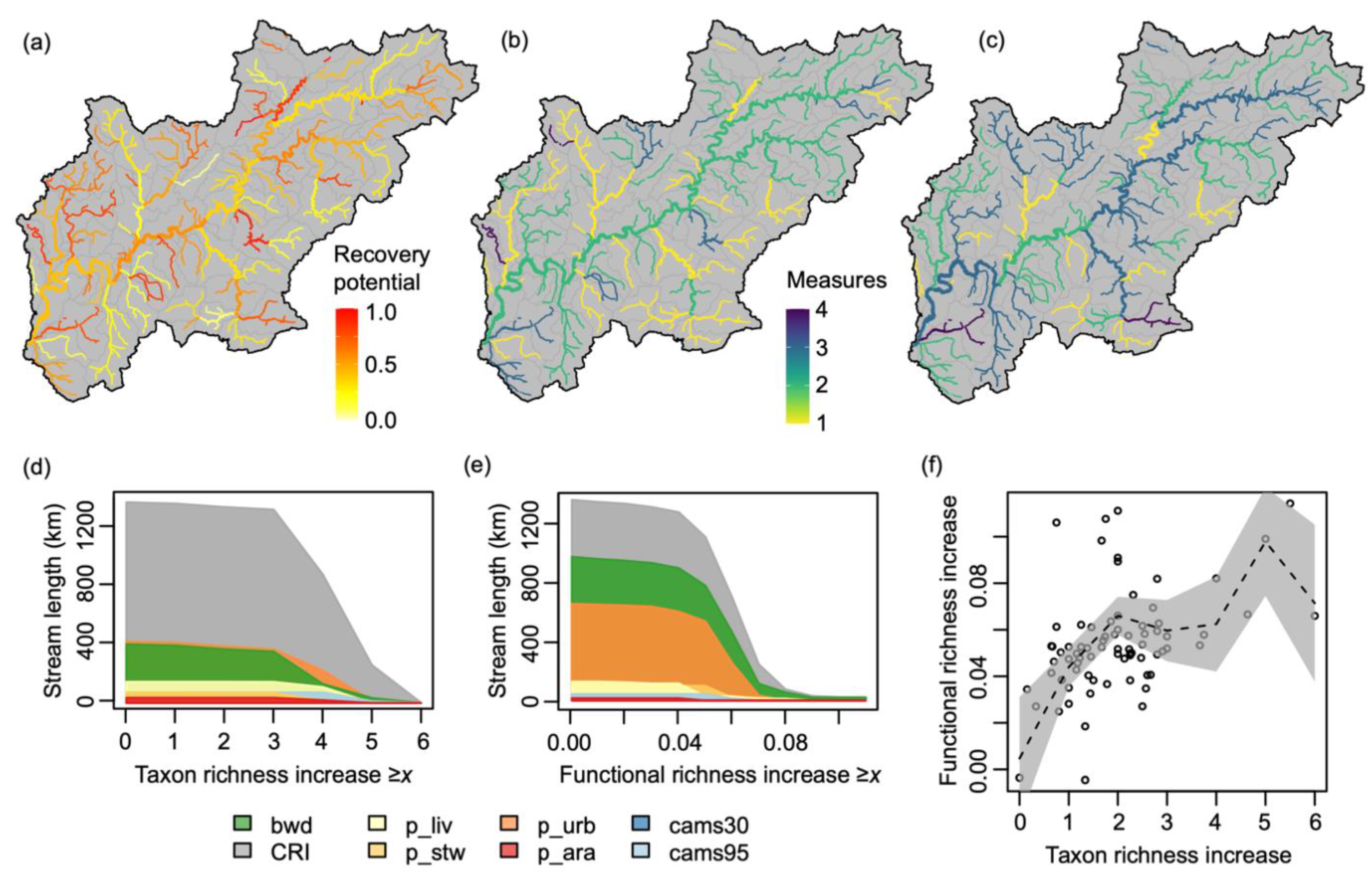
Figure 1. Study location and data availability. (a) Location of the study area. (b) Spatial density of invertebrate community samples used in species distribution modelling. (c) Map of case study catchment. The grey area in (b) shows the Welsh part of the Severn River Basin which was not included in our study.
Water 13 03339 g001
Figure 2. Performance of three alternative species distribution models. Mean evaluation metrics (circles) with taxon prevalence trends (lines) from generalized additive models for (a) mean error (ME), (b) mean absolute error (MAE), (c) true skill statistic (TSS). Models with ME and MAE closer to 0 and TSS values closer to 1 are considered better performing.
Water 13 03339 g002
Figure 3. Summary of predicted responses to four high-level restoration scenarios: riparian woodland creation (“bwd”), removal of channel resectioning (“CRI”), 50% reduction in orthophosphate concentrations from all sources (“p_all”), and abstraction relicensing to bring all water resource availability classifications to “green” status (“cams”). (ae) Predicted change in invertebrate diversity metrics following restoration. (f) Predicted change in mean taxon occurrence probabilities following restoration, with negative responses in red and positive responses in blue.
Water 13 03339 g003
Figure 4. Predicted biodiversity responses to four high-level restoration scenarios: riparian woodland creation (“bwd”), removal of channel resectioning (“CRI”), 50% reduction in orthophosphate concentrations from all sources (“p_all”), and abstraction relicensing to bring all water resource availability classifications to “green” status (“cams”). Baseline taxon richness (a) and functional richness (b) alongside predicted changes following restoration under each scenario. Turnover in species composition (Jaccard dissimilarity) following restoration (c).
Water 13 03339 g004
Figure 5. Recovery potential across the Warwickshire Avon case study catchment. Relative recovery potential of water bodies (a) derived from the ranking of maximum predicted increases in taxon richness and functional richness following restoration. Water bodies with recovery potential closer to 1 are predicted to benefit more from restoration. Number of restoration measures contributing to maximum predicted increases in mean taxon richness (b) and functional richness (c) within water bodies. Stream length predicted to benefit from the inclusion of restoration measures in terms of taxon richness (d) and functional richness (e). Relationship between maximum predicted taxon richness and functional richness increases in each water body (f), with mean and 95% confidence intervals from a generalized additive model. Panels (d,e) show the total stream length predicted to benefit from at least the corresponding level of the biodiversity index for restoration scenarios involving each individual measure. The eight restoration measures included are riparian woodland creation (bwd), removal of channel resectioning (CRI), 50% reduction in orthophosphate concentrations from livestock (p_liv), wastewater treatment (p_stw), urban (p_urb) and arable (p_ara) sources, and abstraction relicensing to bring all water resource availability classifications to “green” status at high flows (cams30) and low flows (cams95).
Water 13 03339 g005
Figure 6. Lower-level restoration measures contributing to recovery potential across the Warwickshire Avon case study catchment: riparian woodland creation (a); removal of channel resectioning (b); 50% reduction in P concentrations from livestock (c), wastewater treatment (d), urban (e) and arable (f) sources; and abstraction relicensing to bring water resource availability classifications to “green” status at low flows (g). All panels show the recovery potential where the corresponding measure contributed to the combination of measures predicted to maximise biodiversity. River segments where the measure did not contribute are plotted in grey.
Water 13 03339 g006
Table 2. Description of restoration scenarios.
Short NameDescription
bwd 1,2Increase broadleaved woodland cover within 1 km of river to 100%
CRI 1,2Remove all elements of channel resectioning (e.g., reinforced bed, banks)
p_all 1Reduce P concentrations from all sources by 50%
p_ara 2Reduce P concentrations from arable sources by 50%
p_liv 2Reduce P concentrations from livestock sources by 50%
p_stw 2Reduce P concentrations from sewage treatment sources by 50%
p_urb 2Reduce P concentrations from urban sources by 50%
cams 1Bring water resource availability classification at both Q30 and Q95 to “green” status
cams30 2Bring water resource availability classification at Q30 to “green” status
cams95 2Bring water resource availability classification at Q95 to “green” status
1 High-level restoration scenarios for which biodiversity responses were predicted individually. 2 Lower-level restoration scenarios for which biodiversity responses were predicted both individually and in combination with other scenarios.
Publisher’s Note: MDPI stays neutral with regard to jurisdictional claims in published maps and institutional affiliations.

