Article

Seasonal Prediction of Summer Precipitation in the Middle and Lower Reaches of the Yangtze River Valley: Comparison of Machine Learning and Climate Model Predictions

1
Changwang School of Honors, Nanjing University of Information Science and Technology, Nanjing 210044, China
2
School of Atmospheric Sciences, Nanjing University of Information Science and Technology, Nanjing 210044, China
3
Key Laboratory of Meteorological Disaster of Ministry of Education/Joint International Research Laboratory of Climate and Environment Change/Collaborative Innovation Center on Forecast and Evaluation of Meteorological Disasters, Nanjing University of Information Science and Technology, Nanjing 210044, China
4
Institute for Climate and Application Research (ICAR), Nanjing University of Information Science and Technology, Nanjing 210044, China
*
Author to whom correspondence should be addressed.
Water 2021, 13(22), 3294; https://doi.org/10.3390/w13223294
Submission received: 22 October 2021 / Revised: 14 November 2021 / Accepted: 17 November 2021 / Published: 21 November 2021

Abstract

:
The middle and lower reaches of the Yangtze River valley (YRV), which are among the most densely populated regions in China, are subject to frequent flooding. In this study, the predictor importance analysis model was used to sort and select predictors, and five methods (multiple linear regression (MLR), decision tree (DT), random forest (RF), backpropagation neural network (BPNN), and convolutional neural network (CNN)) were used to predict the interannual variation of summer precipitation over the middle and lower reaches of the YRV. Predictions from eight climate models were used for comparison. Of the five tested methods, RF demonstrated the best predictive skill. Starting the RF prediction in December, when its prediction skill was highest, the 70-year correlation coefficient from cross validation of average predictions was 0.473. Using the same five predictors in December 2019, the RF model successfully predicted the YRV wet anomaly in summer 2020, although it had weaker amplitude. It was found that the enhanced warm pool area in the Indian Ocean was the most important causal factor. The BPNN and CNN methods demonstrated the poorest performance. The RF, DT, and climate models all showed higher prediction skills when the predictions start in winter than in early spring, and the RF, DT, and MLR methods all showed better prediction skills than the numerical climate models. Lack of training data was a factor that limited the performance of the machine learning methods. Future studies should use deep learning methods to take full advantage of the potential of ocean, land, sea ice, and other factors for more accurate climate predictions.

1. Introduction

The middle and lower reaches of the Yangtze River valley (YRV) are among the most densely populated and economically developed regions in China. With the longest river in Asia flowing through this area, there is a risk of frequent summer floods that can cause substantial damage to infrastructure and threaten livelihoods. Summer precipitation in the YRV is largely the result of moisture transport from the Indian Ocean and the South China Sea [1,2], which has a complex relationship with atmospheric circulations such as the western Pacific subtropical high and East Asian trough [3,4].
To minimize regional damage caused by summer flooding, it is desirable that summer precipitation in the YRV be predicted seasons in advance. However, the current level of prediction accuracy for YRV summer precipitation is only 60–70% [5]. The initial atmospheric state is very important for short-term weather forecast; however, seasonal climate prediction has to consider the slowly evolving states of both the ocean and the land, as well as their interactions with the atmosphere [6,7]. These slowly evolving components of the climate system can shape atmospheric conditions through their interactions with the atmosphere [8].
Early attempts at seasonal climate prediction in the 1960s–1980s were undertaken using statistical methods. Usually, certain important factors were selected based on previous research or following correlation analysis based on Empirical Orthogonal Function or Singular Value Decomposition methods. Then, predictions were performed using models built on the basis of multiple linear regression (MLR) [5] or more sophisticated canonical correlation analysis [9]. Following the development of numerical climate models, especially those coupling ocean circulation models with atmosphere circulation models, seasonal climate predictions have been produced [10,11]. However, owing to the variety of systematic errors of such models, it is necessary to determine the factors limiting the prediction ability based on the dynamics and statistics [12]. There have also been attempts to combine climate model predictions with statistical methods [13], especially for the downscaling of climate model predictions to regional and smaller scales [14].
In recent years, the machine learning approach has been applied to many fields, including earth system science and atmospheric science [15]. The deep learning method has certain advantages for the stochastic analysis of precipitation series [16] and simulation of catchment responses [17]. Some machine learning methods have shown excellent performance in the selection of predictors and in making predictions. The methods used most frequently include the random forest (RF; [18]), support vector machine (SVM; [19]), and various neural network methods [20,21]. These methods determine nonlinear relationships among variables by using large amounts of training data obtained previously through observation, from which nonlinear prediction models can be constructed. The performance of such models certainly depends on the volume and quality of the training data. Moreover, selection of the parameters used in the models is also very important because the characteristics of the parameters can greatly affect model performance. For example, Zhen et al. [22] screened the predictors and used five predictors for final prediction. Ham et al. [21] showed through many experiments that in the convolutional neural network (CNN), the number of the epoch from 600 to 1000 do not affect the prediction skill. The parameters of the machine learning model should be adjusted to fit the purpose of the research.
In this study, we used several machine learning methods to predict summer precipitation in the YRV, including summer 2020, with a focus on the RF method and its parameter settings and predictor selection. The prediction results obtained using the machine learning methods were compared with those derived using the traditional multiple linear regression model and numerical climate models.

2. Data and Prediction Methods

To find an appropriate machine learning method for prediction of summer precipitation in the YRV, it was necessary to first determine the predictors and predictand for the prediction model. Area average precipitation in the YRV was used as the predictand, and the predictors were selected from a collection of atmospheric circulation and sea surface temperature (SST) indexes.

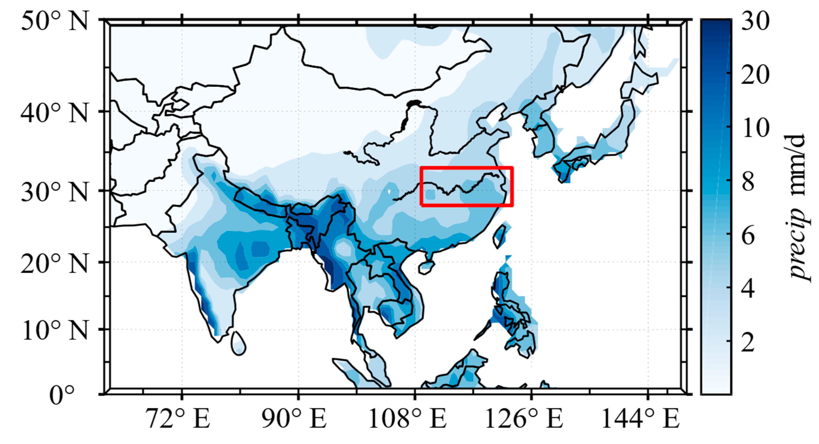
2.1. Precipitation Data

The precipitation data used comprised NOAA’s PRECipitation REConstruction over Land monthly average precipitation (1951–2019) with 1° × 1° resolution ([23]; https://psl.noaa.gov/data/gridded/data.precl.html accessed on 20 April 2021). The area of the YRV was defined as 28°45′–33°25′ N and 110°–123° E. Area average precipitation during June–August in each year was used for the predictand. The climatological mean precipitation from June–August is shown in Figure 1.

2.2. Predictor Data

To select the predictors, we used monthly data from 88 atmospheric circulation indexes, 26 SST indexes, and 16 other indexes (130 indexes in total) obtained from the National Climate Center of China for the period from January 1951 to May 2020 (https://cmdp.ncc-cma.net/Monitoring/cn_index_130.php, accessed on 20 April 2021). The indexes from December of the previous year to May of the current year were used to represent the previous atmospheric circulation and SST conditions. Because some indexes had too many missing records, we removed 20 indexes and retained 110 indexes as the predictors. This should have little effect on the model predictions because many indexes have overlapping information. The data were normalized to be within the range of 0–1. Missing records were ignored in the process of normalization, being assigned a value of 0 so that missing records did not affect the results.

2.3. Climate Model Prediction Data

Hindcast data from global climate models that participated in the North American Multi-Model Ensemble forecasts [10] were used for comparison purposes (https://www.cpc.ncep.noaa.gov/products/NMME/, accessed on 20 April 2021). The model hindcasts started from the first day of each month and extended for 8–12 months, and each hindcast had around 10 ensemble members. Similarly, for the machine learning methods, we used hindcast data with start dates from December of the previous year to May of the current year, and for June–August of each year, the ensemble mean hindcast results were used for evaluation purposes. Eight models that had available data during the common period of 1982–2010 were selected (see Section 4.2). The reader is referred to the above website for further details regarding the climate models.

2.4. Cross Validation of Prediction Results

Owing to the limited length of the observational data set, we used the cross-validation method [24] to take full advantage of the available data. Specifically, there were 70 samples in the original data set (i.e., 1951–2020). Data from one year were used as validation data, and the data from the remaining 69 years were used as training data. In this way, the predictors with the greatest impact on summer precipitation in the YRV were determined and 69 prediction models were constructed. The performance of each of the summer precipitation prediction models was analyzed comprehensively.

2.5. Prediction Methods

In this study, the prediction model was largely based on the RF model, which is an extension of the decision tree (DT) model. Therefore, the basic concept of the DT is introduced first, and then a brief description of the RF procedure is presented. Brief introductions are also provided regarding two neural network models: the backpropagation neural network (BPNN) and the convolutional neural network (CNN). Additionally, we also used the traditional multiple linear regression (MLR) model.

2.5.1. Decision Tree (DT)

The DT is both a classification and a regression method. It is called a classification tree when used for classification and a regression tree when used for regression. The classification and regression tree (CART) is one of the DT algorithms used most frequently for both classification and regression [25]. The CART produces a conditional probability distribution of the departure of a variable for the given predictors. In this study, the DT prediction model was based on the CART, whereby the characteristic input space, composed of predictors, was divided into a finite number of subunits for which the probability distribution of precipitation was determined. Thus, the conditional probability distribution of precipitation could be determined by the given predictors.

2.5.2. Random Forest (RF)

The RF is a machine learning algorithm that combines multiple CARTs to construct the RF and summarizes the results of multiple classifiable regression trees. The RF method was proposed by [26]. Its basic structure is that of a DT and it belongs to the ensemble learning branch of machine learning. The RF is constructed from a combination of CARTs and the set can be visualized as a forest of unrelated DTs. In this study, we divided the predictors and YRV precipitation into a training set and a test set, and the training set was used to train the RF model to form a regressor. The predictors in the test set were input into the regressor, which votes according to the attributes of the predictors. The result of the final prediction can be obtained from the mean value of precipitation derived from the regressor, corresponding to the attributes with the most votes. The construction of the model is described in detail below
The RF method comprises three steps: random sample selection, which is mainly to process the input training set, the RF split algorithm, and output of the predicted result. A flow chart of RF is shown in Figure 2. n denotes the number of decision trees or weak regressors and the experiment in the following paper shows that the efficiency is the highest when n = 200. m denotes the number of predictors to be put into a weak regressor. Since RF is random sampling, the number of predictors put into each weak regressor is smaller than the total number in the initial training set.

2.5.3. Backpropagation Neural Network (BPNN)

A BPNN is a multilayer feed-forward artificial neural network trained using an error backpropagation algorithm [27]. Its structure usually includes an input layer, an output layer, and a hidden layer. It is composed of two processes operating in opposite directions, i.e., the signal forward transmission and error backpropagation.
In the process of forward transmission, the input predictor signals pass through the input layer, hidden layer, and output layer sequentially, a structure called topology. They are implemented in a fully connected mode. In the process of transmission, the signal is processed by each hidden layer. When the actual output of the output layer is not consistent with the expected anomaly, it goes to the next process, i.e., error backpropagation.
In the process of error backpropagation, the errors between the actual output and the expected output are distributed to all neurons in each layer through the output layer, hidden layer, and input layer. When a neuron receives the error signal, it reduces the error by modifying the weight and the threshold values.
The two processes are iterated continuously, and the output is stopped when the error is considered stable.

2.5.4. Convolutional Neural Network (CNN)

A CNN is a variant of the multilayer perceptron that was developed by biologists [28] in a study on the visual cortex of cats. The basic CNN structure consists of an input layer, convolution layers, pooling layers, fully connected layers, and an output layer. Generally, there are several alternating convolution layers and pool layers, i.e., a convolution layer is connected to a pool layer, and the pool layer is then connected to a convolution layer. Because each neuron on the output feature plane in the convolution layer is locally connected to its input, and the input value is obtained by weighted summation of the corresponding connection weight with the local input plus a bias value, this process is equivalent to a convolution process.

2.5.5. Multiple Linear Regression (MLR)

In precipitation forecasts, change in precipitation is often affected by many factors; therefore, it is necessary to use two or more factors to explain changes in precipitation, i.e., multiple regression. When the relationship between multiple predictors and precipitation is linear, the MLR model can be written as follows:
P d e p a r t u r e t = β 0 + β 1 F 1 , t + β 2 F 2 , t + + β n F n , t + e t
where n is the number of factors, t is the year (1951–2019), β i ( i = 0 , 1 , , n ) is the regression coefficient, P d e p a r t u r e t is the predicted precipitation departure, F i , t is the normalized value of the jth ( j = 1 , , n ) predictor and e t is the residual. Using the least squares method to estimate the regression coefficients and residuals, the optimal MLR model can be obtained.

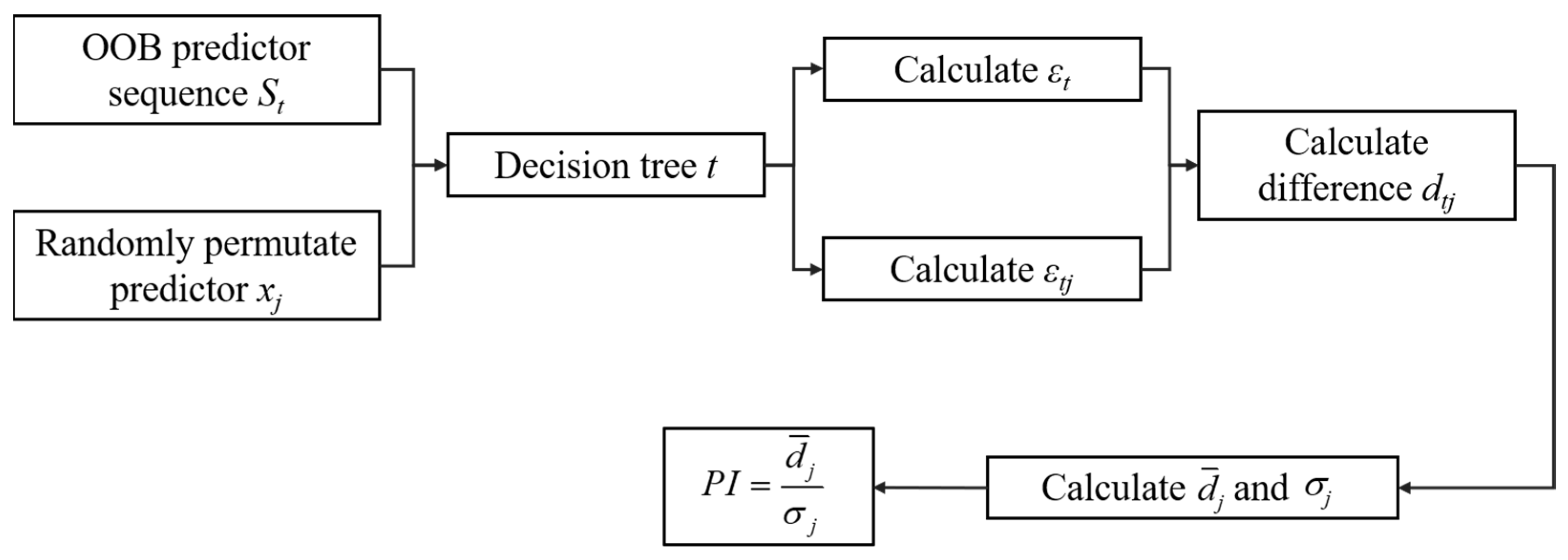
3. Predictor Importance Analysis Model (PIAM)

In this study, not all 110 predictors were included in the prediction model. After deleting 20 predictors with over 15 years of missing data, there were 90 predictors remaining. To select the predictors that are most useful for the prediction model, we used the predictor importance analysis model (PIAM), which is based on bagging and out-of-bagging (OOB) data [29]. OOB data are those samples that are not selected in bootstrap sampling at a particular time, which account for 36.8% of the total samples if the data set has a sufficient number of samples, and they can be used to calculate the importance of predictors for the prediction model.
Determination of the importance of the predictors for the purpose of predictor selection is calculated via random permutation of OOB data. Here, random permutation means that the values of the predictors from different years of OOB data are randomly disturbed. Then, they are put into weak regressors for precipitation prediction, and the difference between the forecast value and the actual observed value is calculated. In this step, an element of OOB data corresponds to either a weak regressor or a regression tree. If a predictor has substantial influence on the prediction result, the random arrangement will also have an evident effect on the prediction error; otherwise, it will have almost no effect.
The following is a detailed description of the operation process of the measurement of importance of a predictor based on OOB data, where R is a weak regression of the RF that contains T DTs and P is the number of predictors in the training data set. A flow chart of PIAM is shown in Figure 3.
  • For DT t , where t = 1 , , T :
    (a)
    Determine the observation of OOB data (precipitation anomaly) and the value of the predictors. These OOB data sets will be input into the DT. Denote the sequence of predictors as s t { 1 , , P } ;
    (b)
    Calculate the root mean square error ( ε t ) of the OOB data;
    (c)
    For predictor x j , j s t :
    • Randomly permutate the observation of predictor x j ;
    • Put the observation into the weak regressor and calculate the prediction error ε t j of the model;
    • Calculate the difference d t j = ε t j ε t between cases without or with permutation. If predictor x j has little impact on the prediction model, d t j will be relatively small and its absolute value will be close to 0.
  • For difference d t j , calculate the average d ¯ j and the standard deviation σ j .
  • Finally, predictor importance can be calculated as P I = d ¯ j σ j .
To verify the PIAM performance, we selected three typical years of major floods in the YRV (1954, 1998, and 2020) for analysis. First, we calculated the importance of each predictor in the three years and sorted them accordingly. The performance of the importance analysis models was verified using the P I values and the results of previous analyses of the precipitation mechanism conducted in other studies.
Bar plots of the P I values for each of the three selected years and the entire 70-year period are shown in Figure 2, where the data of the predictors in the previous December are selected. Using P I = 0.15 as the threshold (red line in Figure 4), 14, 9, and 6 predictors can be selected for 1954, 1998, and 2020, respectively, whereas only 4 predictors pass the threshold for all 70 years of data period. Therefore, although the relative importance of the predictors varies between years, there are four outstanding predictors for all 70 years of data, indicating that these four predictors affect YRV precipitation in most years.
The top 10 predictors are shown in Figure 5 after the PI values were arranged in descending order. In relation to the abnormal precipitation in the YRV in summer 1954, PIAM selected predictors that included Pacific Ocean SST, the western Pacific subtropical high ridge line, and the polar vortex (Figure 5a). In July, the mid-latitudes were dominated by a blocking high over the Sea of Okhotsk and the Ural Mountains. Before July, the position of the western Pacific subtropical high in the southeast was further south than normal [30]. In early July, the western Pacific subtropical high extended to the north of 25° N before retreating southward again by the middle of July. Moreover, El Niño occurred in the eastern equatorial Pacific Ocean from 1953–1954 and Pacific Ocean SST became abnormally warm [30]. Therefore, for 1954, the PIAM accurately selected the most important predictors of summer precipitation in the YRV.
Overall, the case of 1998 is similar to that of 1954, except that the first two major predictors of YRV precipitation in 1998 are both NINO SST indexes, and the third predictor is the western Pacific subtropical high index (Figure 5b). This is related to the unusually strong El Niño that occurred in 1998. A strong El Niño event affects the mid-latitude circulation, making the occurrence of blocking highs more likely, such that YRV precipitation is enhanced [30]. This indicates that the PIAM can identify the most important predictors in particular years.
The precipitation that occurred in the YRV in 2020 was anomalous. In April 2020, most forecast models predicted that there would not be much precipitation in the flood season of 2020, which was contrary to reality. The warm tropical Indian Ocean was the main cause of the heavy rainfall in the YRV during June–July 2020 [31], which is inconsistent with the prevailing opinion that summer precipitation in the YRV is influenced mainly by the western Pacific subtropical high. This might also be one of the reasons for the poor prediction regarding YRV precipitation in 2020. However, the PIAM selected the Indian Ocean warm pool area index as the second most important predictor (Figure 5c), indicating that the model has certain generalization capability. The wind speed index and the Northern Hemisphere circulation index were also screened out, and the quasi-biweekly oscillation of the atmospheric circulation and low-level jet in the southwest causes the Meiyu front to persist for a long time, which is also consistent with the PIAM results [32].
Of the four predictors screened out for the entire 70-year period (Figure 5d), those other than the North American polar vortex index are known to influence precipitation in the YRV, e.g., the NINO index and zonal circulation index.
The PIAM results show that the model based on bagging and OOB data has certain generalization capability and can accurately screen out the predictors that affect summer precipitation in the YRV in each year. Thus, it could represent the foundation for accurate prediction by a model based on machine learning.

4. Precipitation Prediction Based on Machine Learning

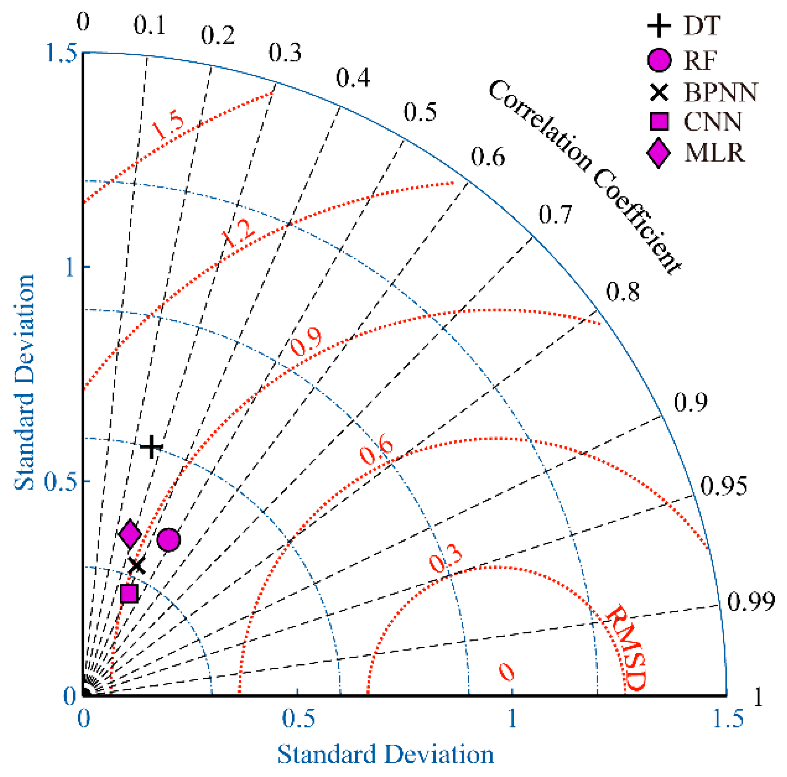
4.1. Comparison of Five Machine Learning Methods

To compare the performances of various machine learning methods, we selected five machine learning methods. Because the predictors in different months have different degrees of influence on YRV summer precipitation, the month with the best forecast effect should be determined first. The high-latitude circulation and snow cover of the Tibetan Plateau in early winter might have considerable influence on summer precipitation in the YRV [33]. Similarly, SST in early spring might also influence summer precipitation in the YRV [34], especially in the year following an El Niño event [33].
In this study, OOB data were used to sort the importance of the forecast factors, but the number of predictors was not given explicitly. This is because different prediction models might perform better with different numbers of predictors. Therefore, the most critical parameters for each model are the start time and the number of predictors.
The MLR model is the simplest, with only two parameters that need to be adjusted. The DT method needs the number of DTs to be determined. The RF method needs the minimum number of leaf nodes to be determined. A BPNN needs the number of hidden layers and the number of neurons in each hidden layer to be determined. A CNN needs the number of convolutional layers and pooling layers, the small batch number, and the learning rate to be determined. After preliminary experiments, the optimal selection of parameters for each precipitation forecast model was obtained, as shown in Table 1.
The selected parameter settings were brought into each prediction model and a Taylor diagram was plotted for statistical comparison of the results of the five methods with observed precipitation (Figure 6). In terms of standard deviation, the DT model is closest to 1 and the CNN performs worst. The RF model has the highest correlation coefficient, while those of the CNN and BPNN are the lowest. In terms of the root mean square error, the RF and DT models have the smallest and largest values, respectively. The performance of the MLR model is relatively poor, i.e., the traditional linear model takes the least amount of time, but its prediction skill is not as good as that of the nonlinear models. It can be seen in Figure 4 that the RF model plots closest to the center of the circle in the lower-right corner of the Taylor diagram, which indicates that the RF model performs best among the five methods tested.

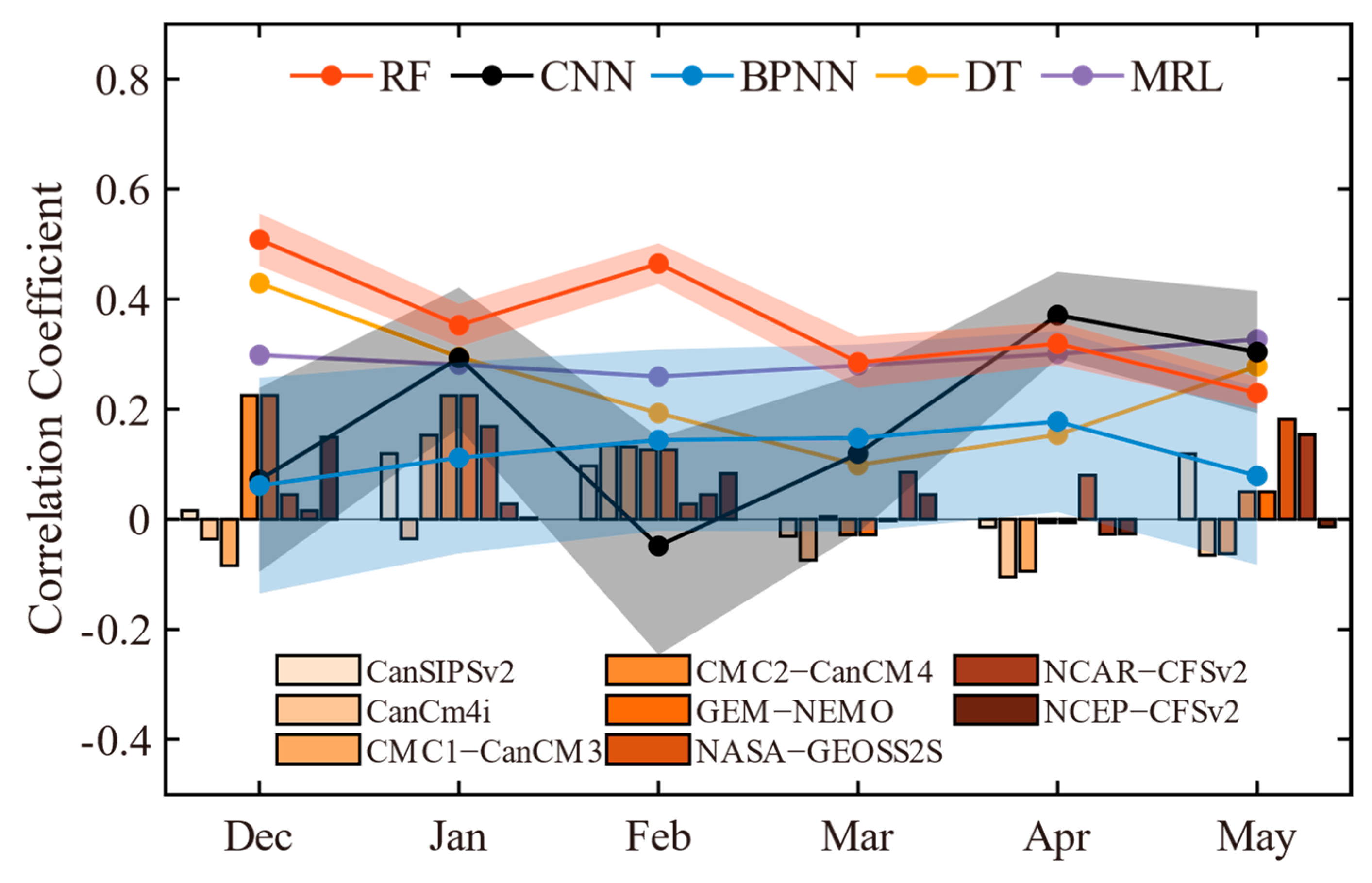
4.2. Comparison of Machine Learning Methods and Numerical Model Simulations

Because the periods of the prediction experiments were different for the different numerical models, the years in common with the prediction results of the unified model were selected, i.e., 1982–2010. Machine learning methods have certain randomness, which means that they need many experimental iterations for statistical analysis to reflect the generalization capability of the machine learning model. The results of YRV summer precipitation forecasts, illustrated in Figure 7, show the correlation coefficients obtained from cross validation between the machine learning models and the predictions of the numerical models.
First, the predictions of the DT and MLR models do not have spread (Figure 7). This is because the selection of the DT split node is fixed without randomness such that the prediction results are the same every time. For the MLR model, the selection of predictors and the regression coefficient calculated using the least squares method are fixed; therefore, the forecast result does not change. The results of the RF, BPNN, and CNN models each have a certain amount of spread. The spread of the RF model is much smaller than that of either of the two neural network methods, which indicates that its uncertainty is smaller. For the neural network methods, the CNN performs better and has less uncertainty than the BPNN. The network structure of the CNN is much more complex than that of the BPNN, which means that more information can be obtained from the predictors.
The bar chart in Figure 7 shows the precipitation prediction results of eight climate models. The prediction skill of each is not as good as that of the RF model. The prediction results of the RF and DT models show that the predictors in December can better predict summer precipitation in the YRV, while CNN and BPNN have better prediction skills in April. Overall, all the climate models show higher prediction skill when the predictions start in winter than in early spring. This is related to the so-called “spring predictability barrier,” which might reflect the fact that the ocean–atmosphere system is most unstable in spring and therefore prone to error growth [7,35].

4.3. Cross Validation Prediction Results Analysis of Optimal Method

The RF prediction model demonstrated superior performance and therefore it was selected as the optimal machine learning model for further study. The forecast skill of the RF model when run with different start times and increasing numbers of predictors is shown in Figure 8. The prediction skill is high in December with only two predictors but lower with 3–7 predictors, indicating that consideration of any additional predictor greatly interferes with the predictive power of the first two predictors. However, when the eighth predictor is added, the decreasing trend in model prediction skill is alleviated, which means that this predictor has strong predictive information. With 8–14 predictors, the prediction skill of the RF model increases with the increasing number of predictors. The prediction skill of the model reaches its peak with 14 predictors, and consideration of any additional predictors only diminishes the prediction skill at a small rate.
To obtain the best performance from the RF model, the stepwise regression method was used to further screen the 14 predictors. Stepwise regression has the advantage of selecting predictors with less interdependence. Therefore, the PIAM was used to select those predictors containing the strongest prediction signals, and stepwise regression was used to obtain the optimal combination of those predictors.
Using the stepwise regression method, the forecast results were plotted according to the number of different predictors, as shown in Figure 9. The correlation coefficient and root mean square error of the model both reached the optimal level when there were five predictors in December; the prediction performance changed little with further increases in the number of predictors. In May, the forecast results were best when there were two forecast factors, but the performance was not as good as that achieved in December. Therefore, the five important predictors in December were used for cross-validation purposes, and their average value was obtained through 500 tests (Figure 10). The 70-year cross validation produced a correlation coefficient of 0.473 and a root mean square error of 0.852.
Five predictors in December 2019 were used to predict the summer precipitation in the YRV in 2020. It can be seen from Figure 10 that the RF model predicted an abnormal increase in summer precipitation in the YRV in 2020. Considering the forecast factors for 2020 screened out in Section 3, it can be determined that the high precipitation in summer 2020 was related to the Indian Ocean SST, which is consistent with the conclusion of Tang et al. [31].
It can be seen that the prediction ability of the model before 1980 is not as good as that after 1980 (Figure 10). The greater volume of satellite-derived observational data after 1980 improved the accuracy of atmospheric fields, which improved the accuracy of the observational and re-analysis datasets. Therefore, the data available after 1980 were more consistent with the actual situation and could better reflect the physical mechanisms behind the predictors. The better model initialization also improved the prediction accuracy.

5. Summary and Conclusions

The RF and three other machine learning methods and the MLR model were used to predict summer precipitation in the YRV. Five predictors were selected from 130 circulation and SST indexes using RF and stepwise regression methods. It was found that the RF model had the best performance of all the tested statistical methods. Starting the RF prediction in December, when its prediction skill was highest, the 70-year correlation coefficient from cross validation of the average predictions reached 0.476. The CNN and BPNN methods produced the poorest performance. It was also found that the predictive performance of the RF, DT, and MLR models was better than that of the numerical climate models. Moreover, the RF, DT, and numerical models all showed higher prediction skills when the predictions start in winter than in early spring. Using five predictors in December 2019, the RF model successfully predicted the wet anomaly in the YRV in summer 2020 but with weaker amplitude. It was established that the warm pool area in the Indian Ocean might be the most important causal factor regarding this precipitation anomaly.
The reasonable performance of the RF model in predicting the anomalies is related to its voting method, but the voting of multiple DTs will smooth out extreme cases; therefore, its prediction capability for extreme precipitation is poorer. The DT prediction model is better for the prediction of extreme values, but it has large biases in years when precipitation anomalies or related circulation and SST features are not strong. The poor predictive ability of the two neural network methods might reflect the fact that only certain indexes are used as predictors and that the deep learning capabilities of neural network methods over the space are not fully exploited. Moreover, the small amount of training data might have limited the performance of the neural network methods.
Although the 130 indexes reflect the main features of the atmospheric circulations and SST, certain potentially important factors were not considered. For example, initial land surface soil moisture, vegetation, snow, and sea ice states have been shown capable of enhancing seasonal prediction skill (e.g., [36,37,38,39]); however, they were not considered in this study. We only considered those indexes related to SST, which might not contain sufficient information regarding the ocean heat content and its memory. Future studies should use deep learning methods to take full advantage of the potential of ocean, land, sea ice, and other factors for producing more accurate climate predictions.

Author Contributions

Conceptualization, C.H. and J.W.; methodology, C.H and J.W.; software, C.H.; formal analysis, C.H. and Y.S.; writing—original draft preparation, C.H. and J.W.; writing—review and editing, J.W. and J.-J.L.; funding acquisition, J.W. and J.-J.L. All authors have read and agreed to the published version of the manuscript.

Funding

This research was supported by National Key Research and Development Program of China (Grant 2020YFA0608004) and Jiangsu Department of Education, China.

Institutional Review Board Statement

Not applicable.

Informed Consent Statement

Not applicable.

Data Availability Statement

The data presented in this study are available on request from the corresponding author.

Acknowledgments

We thank James Buxton, for editing the English text of a draft of this manuscript.

Conflicts of Interest

The authors declare no conflict of interest.

References

  1. Ronghui, H.; Zhenzhou, Z.; Gang, H. Characteristics of the Water Vapor Transport in East Asian Monsoon Region and Its Difference from That in South Asian Monsoon Region in Summer. Sci. Atmos. Sin. 1998, 22, 76–85. (In Chinese) [Google Scholar]
  2. Wei, J.; Dirmeyer, P.A.; Bosilovich, M.G.; Wu, R. Water Vapor Sources for Yangtze River Valley Rainfall: Climatology, Variability, and Implications for Rainfall Forecasting. J. Geophys. Res. Atmos. 2012, 117, 1–11. [Google Scholar] [CrossRef]
  3. Ding, Y.; Sun, Y.; Wang, Z.; Zhu, Y.; Song, Y. Inter-Decadal Variation of the Summer Precipitation in China and Its Association with Decreasing Asian Summer Monsoon Part II: Possible Causes: Possible Causes for Inter-Decadal Variation in Summer Precipitation in China. Int. J. Climatol. 2009, 29, 1926–1944. [Google Scholar] [CrossRef]
  4. Yihui, D.; Chan, J.C.L. The East Asian Summer Monsoon: An Overview. Meteorol. Atmos. Phys. 2005, 89, 117–142. [Google Scholar] [CrossRef]
  5. Ke, F.; Jun, W.H.; Jean, C.Y. A Physically-Based Statistical Forecast Model for the Middle-Lower Reaches of the Yangtze River Valley Summer Rainfall. Chin. Sci. Bull. 2008, 53, 602–609. (In Chinese) [Google Scholar] [CrossRef]
  6. Dirmeyer, P.A.; Fennessy, M.J.; Marx, L. Low Skill in Dynamical Prediction of Boreal Summer Climate: Grounds for Looking beyond Sea Surface Temperature. J. Clim. 2003, 16, 995–1002. [Google Scholar] [CrossRef]
  7. Duan, W.; Wei, C. The ‘spring predictability barrier’ for ENSO predictions and its possible mechanism: Results from a fully coupled model. Int. J. Climatol. 2013, 33, 1280–1292. [Google Scholar] [CrossRef]
  8. Dickinson, R.E. How Coupling of the Atmosphere to Ocean and Land Helps Determine the Timescales of Interannual Variability of Climate. J. Geophys. Res. 2000, 105, 20115–20119. [Google Scholar] [CrossRef]
  9. Barnston, A.G.; Smith, T.M. Specification and Prediction of Global Surface Temperature and Precipitation from Global SST Using CCA. J. Clim. 1996, 9, 2660–2697. [Google Scholar] [CrossRef] [Green Version]
  10. Kirtman, B.P.; Min, D.; Infanti, J.M.; Kinter, J.L.; Paolino, D.A.; Zhang, Q.; Van Den Dool, H.; Saha, S.; Mendez, M.P.; Becker, E.; et al. The North American Multimodel Ensemble: Phase-1 Seasonal-to-Interannual Prediction; Phase-2 toward Developing Intraseasonal Prediction. Bull. Am. Meteorol. Soc. 2014, 95, 585–601. [Google Scholar] [CrossRef]
  11. Shukla, J.; Anderson, J.; Baumhefner, D.; Brankovic, C.; Chang, Y.; Kalnay, E.; Marx, L.; Palmer, T.; Paolino, D.; Ploshay, J.; et al. Dynamical Seasonal Prediction. Bull. Am. Meteorol. Soc. 2000, 81, 2593–2606. [Google Scholar] [CrossRef]
  12. Doblas-Reyes, F.J.; García-Serrano, J.; Lienert, F.; Biescas, A.P.; Rodrigues, L.R.L. Seasonal Climate Predictability and Forecasting: Status and Prospects. WIREs Clim. Chang. 2013, 4, 245–268. [Google Scholar] [CrossRef]
  13. Luo, L.; Wood, E.F.; Pan, M. Bayesian Merging of Multiple Climate Model Forecasts for Seasonal Hydrological Predictions: Bayesian seasonal hydrologic predictions. J. Geophys. Res. 2007, 112. [Google Scholar] [CrossRef] [Green Version]
  14. Li, X.; Babovic, V. Multi-Site Multivariate Downscaling of Global Climate Model Outputs: An Integrated Framework Combining Quantile Mapping, Stochastic Weather Generator and Empirical Copula Approaches. Clim. Dyn. 2019, 52, 5775–5799. [Google Scholar] [CrossRef]
  15. Reichstein, M.; Camps-Valls, G.; Stevens, B.; Jung, M.; Denzler, J.; Carvalhais, N.; Prabhat. Deep Learning and Process Understanding for Data-Driven Earth System Science. Nature 2019, 566, 195–204. [Google Scholar] [CrossRef] [PubMed]
  16. Rozos, E.; Dimitriadis, P.; Mazi, K.; Koussis, A.D. A Multilayer Perceptron Model for Stochastic Synthesis. Hydrology 2021, 8, 67. [Google Scholar] [CrossRef]
  17. Kratzert, F.; Klotz, D.; Shalev, G.; Klambauer, G.; Hochreiter, S.; Nearing, G. Towards Learning Universal, Regional, and Local Hydrological Behaviors via Machine Learning Applied to Large-Sample Datasets. Hydrol. Earth Syst. Sci. 2019, 23, 5089–5110. [Google Scholar] [CrossRef] [Green Version]
  18. Li, L.; Schmitt, R.W.; Ummenhofer, C.C.; Karnauskas, K.B. Implications of North Atlantic Sea Surface Salinity for Summer Precipitation over the U.S. Midwest: Mechanisms and Predictive Value. J. Clim. 2016, 29, 3143–3159. [Google Scholar] [CrossRef] [Green Version]
  19. Pham, Q.; Yang, T.-C.; Kuo, C.-M.; Tseng, H.-W.; Yu, P.-S. Combing Random Forest and Least Square Support Vector Regression for Improving Extreme Rainfall Downscaling. Water 2019, 11, 451. [Google Scholar] [CrossRef] [Green Version]
  20. Gentine, P.; Pritchard, M.; Rasp, S.; Reinaudi, G.; Yacalis, G. Could Machine Learning Break the Convection Parameterization Deadlock? Geophys. Res. Lett. 2018, 45, 5742–5751. [Google Scholar] [CrossRef]
  21. Ham, Y.G.; Kim, J.H.; Luo, J.J. Deep Learning for Multi-Year ENSO Forecasts. Nature 2019, 573, 568–572. [Google Scholar] [CrossRef]
  22. Yiwei, Z.; Min, H.; Baohong, L.; Jian, Z.; Huan, L. Research of Medium and Long Term Precipitation Forecasting Model Based on Random Forest. Water Resour. Power 2015, 33, 6–10. (In Chinese) [Google Scholar]
  23. Chen, M.; Xie, P.; Janowiak, J.E. Global Land Precipitation: A 50-Yr Monthly Analysis Based on Gauge Observations. J. Hydrometeorol. 2002, 3, 249–266. [Google Scholar] [CrossRef]
  24. Browne, M.W. Cross-Validation Methods. J. Math. Psychol. 2000, 44, 108–132. [Google Scholar] [CrossRef] [Green Version]
  25. Breiman, L.; Friedman, J.H.; Olshen, R.A.; Stone, C.J. Classification and Regression Trees. Int. Biom. Soc. 1983, 40, 874. [Google Scholar] [CrossRef] [Green Version]
  26. Breiman, L. Random Forests. Mach. Learn. 2001, 45, 5–32. [Google Scholar] [CrossRef] [Green Version]
  27. Rumelhart, D.E.; Hinton, G.E.; Williams, R.J. Learning Representations by Back-Propagating Errors. Nature 1986, 323, 533–536. [Google Scholar] [CrossRef]
  28. Hubel, D.H.; Wiesel, T. Receptive Fields, Binocular Interaction and Functional Architecture in the Cat’s Visual Cortex. J. Physiol. 1962, 160, 106–154. [Google Scholar] [CrossRef]
  29. Breiman, L. Bagging Predictors. Mach. Learn. 1996, 24, 123–140. [Google Scholar] [CrossRef] [Green Version]
  30. Yongling, Z.; Shengan, W.; Yuguo, D.; Tong, H.; Quanzhou, G. Forecast of Summer Precipitation Based on SVD Iteration Model. Acta Meteorol. Sin. 2006, 64, 121–127. (In Chinese) [Google Scholar]
  31. Tang, S.; Luo, J.J.; He, J.; Wu, J.; Zhou, Y.; Ying, W. Toward Understanding the Extreme Floods over Yangtze River Valley in June–July 2020: Role of Tropical Oceans. Adv. Atmos. Sci. 2021, 38, 2023–2039. [Google Scholar] [CrossRef]
  32. Yunyun, L.; Yihui, D. Characteristics and Possible Causes for the Extreme Meiyu in 2020. Meteorol. Mon. 2020, 46, 1393–1404. (In Chinese) [Google Scholar] [CrossRef]
  33. Zhaobo, S. Short-Term Climate Prediction; China Meteorological Press: Beijing, China, 2010; pp. 223–255. (In Chinese) [Google Scholar]
  34. Lei, W.; Renhe, Z.; Jiayou, H. Diagnostic Analyses and Hindcast Experiments of Spring Sst on Summer Precipitation in China. Acta Meteorol. Sin. 2004, 62, 851–859. (In Chinese) [Google Scholar]
  35. Webster, P.J.; Yang, S. Monsoon and Enso: Selectively Interactive Systems. Q. J. R. Meteorol. Soc. 1992, 118, 877–926. [Google Scholar] [CrossRef]
  36. Budikova, D. Role of Arctic Sea Ice in Global Atmospheric Circulation: A Review. Glob. Planet. Chang. 2009, 68, 149–163. [Google Scholar] [CrossRef]
  37. Koster, R.D.; Mahanama, S.P.P.; Yamada, T.J.; Balsamo, G.; Berg, A.A.; Boisserie, M.; Dirmeyer, P.A.; Doblas-Reyes, F.J.; Drewitt, G.; Gordon, C.T.; et al. The Second Phase of the Global Land-Atmosphere Coupling Experiment: Soil Moisture Contributions to Subseasonal Forecast Skill. J. Hydrometeorol. 2011, 12, 805–822. [Google Scholar] [CrossRef]
  38. Lin, P.; Yang, Z.L.; Wei, J.; Dickinson, R.E.; Zhang, Y.; Zhao, L. Assimilating Multi-Satellite Snow Data in Ungauged Eurasia Improves the Simulation Accuracy of Asian Monsoon Seasonal Anomalies. Environ. Res. Lett. 2020, 15. [Google Scholar] [CrossRef]
  39. Pielke, R.A.; Liston, G.E.; Eastman, J.L.; Lu, L.; Coughenour, M. Seasonal Weather Prediction as an Initial Value Problem. J. Geophys. Res. Atmos. 1999, 104, 19463–19479. [Google Scholar] [CrossRef] [Green Version]
Figure 1. Climatological mean precipitation (1951–2019). Red rectangle encloses the YRV region considered in this study.
Water 13 03294 g001
Figure 2. Flow chart of random forest. n denotes the number of decision trees or weak regressors, and m denotes the number of predictors to be put into a weak regressor.
Water 13 03294 g002
Figure 3. Flow chart of PIAM.
Water 13 03294 g003
Figure 4. Predictor importance in (a) 1954, (b) 1998, (c) 2020, and (d) the entire 70-year period.
Water 13 03294 g004
Figure 5. Top 10 predictors in descending order of PI values in (a) 1954, (b) 1998, (c) 2020, and (d) the entire 70-year period.
Water 13 03294 g005
Figure 6. Taylor diagram for the five methods and their comparison with observed precipitation.
Water 13 03294 g006
Figure 7. Correlation coefficients between predicted and observed 1982–2010 interannual YRV summer precipitation. Start dates are from December of the previous year to May of the current year. Shading on the lines indicates the 95% confidence intervals produced by 1000 iterations of the prediction model.
Water 13 03294 g007
Figure 8. Change in predictive ability of the RF prediction model with start time and number of predictors: (a) correlation coefficient and (b) root mean square error (RMSE; mm/day) of the predicted and observed YRV summer precipitation.
Water 13 03294 g008
Figure 9. Results of RF forecasts using different numbers of predictors under stepwise regression.
Water 13 03294 g009
Figure 10. Prediction results of RF models produced by the cross-validation method. Shading around the lines denotes the 95% confidence interval produced by 500 iterations of the prediction models. The prediction for 2020 is shown in green.
Water 13 03294 g010
Table 1. Optimal selection of parameters for the five machine learning methods.
CategoryMethodParameters
Linear ModelMultiple Linear regression1. Predictors: 4.
2. Start time: May.
Nonlinear ModelTree ModelDecision Tree1. Predictors: 7.
2. Start time: December.
3. Decision tree: 138.
Random Forest1. Predictors: 14.
2. Start time: December.
3. Weak regressor: 180.
4. Minimum leaf node: 8.
Neural NetworkBP Neural Network1. Predictors: 8.
2. Start time: December.
3. Hidden layer: 3.
4. Number of neurons in each hidden layer: 50, 7 and 3.
Convolutional Neural Network1. Predictors: 11.
2. Start time: April.
3. Small batch: 200.
4. Learning rate: 0.005.
5. Number of neurons per layer: 50.
6. Number of convolution layers and pooling layers: 5.
Publisher’s Note: MDPI stays neutral with regard to jurisdictional claims in published maps and institutional affiliations.

